2.1. Quasi-2-D homogeneous flow over topography

Consider a rapidly rotating system on an $f$-plane (with constant Coriolis parameter $f_0$), where the rotation axis is parallel to gravity. The motion of a homogeneous fluid is sufficiently slow to assume that the hydrostatic approximation holds in the vertical direction (Pedlosky Reference Pedlosky1987), which implies that the velocity components $(u,v)$ in the horizontal plane $(x,y)$ are independent of depth. Thus, the fluid motion is nearly two-dimensional (quasi-2-D). The thickness of the fluid layer $h(x,y)$ is space-dependent owing to the shape of the variable topography and time-independent by using the rigid-lid approximation. From the integrated continuity equation, the horizontal velocities may be defined in terms of a transport function $\psi (x,y,t)$ as

(2.1a,b)\begin{equation} u = \frac{1}{h}\frac{\partial \psi}{\partial y}, \quad v ={-}\frac 1h \frac{\partial \psi}{\partial x}. \end{equation}

The vertical component of the relative vorticity is defined as $\omega (x,y,t)=\partial v/\partial x - \partial u/\partial y$. It is easily verified that

(2.2)\begin{equation} \omega ={-}\frac{1}{h}\nabla^{2} \psi + \frac{1}{h^{2}} \boldsymbol{\nabla} h \boldsymbol{\cdot}\boldsymbol{\nabla} \psi, \end{equation}

where $\nabla ^{2}=\partial ^{2}/\partial x^{2} + \partial ^{2}/\partial y^{2}$ is the Laplacian. The relative vorticity equation is

(2.3)\begin{equation} \frac{\partial \omega}{\partial t} + J\left( \frac {\omega+f_0}{h},\psi \right) = \nu \nabla^{2} \omega, \end{equation}

where $J(a,b)=(\partial a/\partial x)(\partial b/\partial y)-(\partial a/\partial y)(\partial b/\partial x)$ is the Jacobian operator and $\nu$ is a viscous coefficient. In the context of laboratory experiments, $\nu$ is the molecular viscosity; for geophysical flows, this parameter is a turbulent coefficient. The potential vorticity is

(2.4)\begin{equation} q=\frac{\omega+f_0}{h}. \end{equation}

In the absence of viscous effects, the vorticity equation transforms into

(2.5)\begin{equation} \frac{\partial q}{\partial t} + u\frac{\partial q}{\partial x} + v \frac{\partial q}{\partial y} = 0, \end{equation}

which expresses the material conservation of $q$. Note that we will ignore any external forcing at the upper surface and friction effects at the solid bottom. Additionally, recall that the SW formulation admits significant depth changes owing to the topography, while the traditional QG model demands that such changes must be much smaller than the mean fluid depth (Grimshaw et al. Reference Grimshaw, Tang and Broutman1994). For non-rotating systems ($\,f_0=0$), the dynamical model (2.1a,b)–(2.3) is equivalent to the ‘lake equations’ (see e.g. Camassa, Holm & Levermore Reference Camassa, Holm and Levermore1997).

2.2. Topography and initial conditions

We consider an axisymmetric submarine mountain centred at the origin. The topography has a Gaussian shape, such that the fluid depth is

(2.6)\begin{equation} h(r)=H-H_m \exp({-r^{2}/R_m^{2}}), \end{equation}

where $r^{2}=x^{2}+y^{2}$, $H$ is the maximum depth (away from the mountain), $H_m$ is the height of the topography and $R_m$ is its radial scale.

Using polar coordinates $(r,\theta )$, the initial dipolar condition is the well-known Chaplygin–Lamb vortex (Meleshko & van Heijst Reference Meleshko and van Heijst1994), whose vorticity distribution inside a circle with radius $a$ is

(2.7)\begin{equation} \omega(r,\theta) ={-}\frac{2U s_l}{a\textrm{J}_0(s_l)} \textrm{J}_1(s_lr/a)\sin\theta, \quad r\leqslant a \end{equation}

and $\omega =0$ for $r>a$. Here, $\textrm {J}_0$ and $\textrm {J}_1$ are Bessel functions of the first kind. The constant $s_l=3.8317$ is the smallest root of $\textrm {J}_1$, that is, $\textrm {J}_1(s_l)=0$. The dipole is symmetrical and travels along the positive $x$-direction at a constant speed $U>0$. The initial position of the dipole is $(x_0,y_0)$ with $x_0<0$, so the vortex approaches the submarine mountain. 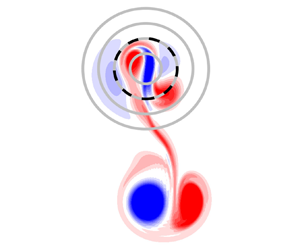In some cases we explored the frontal collision ($y_0=0$) and in some others the dipole trajectory was not aligned with the mountain ($y_0 \neq 0$). Figure 1 shows a typical configuration in one of the experiments with $y_0>0$. Other useful quantities are the total energy per density (Zavala Sansón, van Heijst & Backx Reference Zavala Sansón, van Heijst and Backx2001)

(2.8)\begin{equation} E_0=\frac{H}{2} \int_0^{2{\rm \pi}} \int_0^{a} (u^{2}+v^{2}) r\,\textrm{d}r\,\textrm{d}\theta = 2{\rm \pi} H a^{2} U^{2}, \end{equation}

and the circulation of the poles (Meleshko & van Heijst Reference Meleshko and van Heijst1994)

(2.9)\begin{equation} \varGamma^{{\pm}}_0=\int_0^{2{\rm \pi}} \int_0^{a} \omega^{{\pm}} r\,\textrm{d}r\,\textrm{d}\theta ={\pm} 6.83Ua, \end{equation}

where symbols $+$ and $-$ indicate positive and negative values. Because the initial dipole is symmetric, we define $\varGamma _0\equiv \varGamma ^{+}_0=|\varGamma ^{-}_0|$.

Figure 1. Experimental configuration. The submarine mountain (2.6) is represented with topography contours (grey circles) centred at the origin. The contours correspond to fluid depth $h(r)$ evaluated at radial distances $(0.5,1,1.5,2)R_m$ (dashed contour corresponds to $h(R_m)$). The dipolar vortex has a radius $a$ and is initially located to the left of the mountain $x_0<0$ at $(x_0,y_0)$ (in this example $y_0>0$). Symbols $\pm$ indicate the vorticity sign at each half of the dipole.

2.3. Outline of numerical experiments

The experiments are designed to study: (i) the effect of the mountain on the structure and trajectory of the dipole, and (ii) the long-term motions generated over the topography. The relevant time scale is the rotation period of the system, $T=4{\rm \pi} /f_0$, which defines one ‘day’. The time step is a small fraction of one day, $\textrm {d}t=0.0239 T$. The duration of the simulations was $71.62$ days (3000 time steps). The interaction of the dipole with the mountain occurs during the first 15 to 20 days, while the long-lived, residual structures are observed during the subsequent 40 to 50 days.

A total of 27 simulations were performed, as indicated in table 1. The horizontal length scales are given in terms of the vortex radius $a$, and the vertical ones are compared with the total depth $H$. The experiments are identified with the nomenclature $A_{ij},B_{ij},C_{ij}$. Characters $A,B,C$ define the type of collision according to three different values of $y_0/a$. Subscript $i=1,2,3$ indicates three values of the mountain height $H_m/H$. Subscript $j=1,2,3$ corresponds to three mountain radii $R_m/a$. For instance, the case shown in figure 1 corresponds to experiment $B_{22}$: a ‘northern’ collision against a mountain with medium height and medium width ($y_0/a=1,H_m/H=0.3,R_m/a=2$). All simulations were performed within a square, closed box of side $L \times L$ with $L=20a$. Note that the domain size is several times larger than the size of the dipole and the horizontal scale of the mountain, $L\gg a,R_m$. The vortex is initially located in the $x$-direction at $x_0=-L/3=-6.667a$. Because the dipole moves initially towards the centre of the domain, the vortex-mountain interaction takes place far from the (no-slip) lateral walls.

Table 1. Outline of the 27 numerical simulations. The sets of experiments are identified according to a matrix nomenclature: for instance, experiment $A_{11}$ corresponds to $y_0/a=0,H_m/H=0.1,R_m/a=0.15$.

The speed of the dipole is almost one vortex radius per day, $U=0.84a/T$. Thus, from (2.8) the energy is $E_0=4.43Ha^{4}/T^{2}$. From (2.9), the absolute-value circulation in each of the parts is $\varGamma _0=5.74 a^{2}/T$. The viscous coefficient is set to obtain a Reynolds number of $Re=Ua/\nu = 1500$, while the Rossby number is $Ro=U/f_0a = 0.067$. Thus, the initial vortex resembles a nearly inviscid, slowly moving vortex. These numbers are attainable in laboratory experiments in a rotating table, while being sufficiently adequate to explore the dynamics of geophysical cases. For instance, typical values of experimental dipoles in a rotating tank with tap water are $f_0=1\ \textrm {s}^{-1}$, $\nu =10^{-6}\ \textrm {m}^{2}\ \textrm {s}^{-1}$, $a=0.15$ m, $U=0.01$ ms$^{-1}$ (Zavala Sansón et al. Reference Zavala Sansón, van Heijst and Backx2001; Tenreiro et al. Reference Tenreiro, Zavala Sansón and van Heijst2006). Maximum depths $H$ in different experimental arrangements range between 0.2 and 1 m (Zavala Sansón & van Heijst Reference Zavala Sansón and van Heijst2014).

2.4. Numerical method

The numerical scheme is a finite differences code that has been used in several previous works of experimental rotating flows over topography (Zavala Sansón & van Heijst Reference Zavala Sansón and van Heijst2014). The code was originally developed by R. Verzicco and P. Orlandi for two-dimensional flows (Orlandi Reference Orlandi1990) and later extended to include rotation effects by J. van Geffen. Further modifications were included by Zavala Sansón & van Heijst (Reference Zavala Sansón and van Heijst2002) to account for variable topography effects and Ekman friction. For a homogeneous fluid, the code solves the vorticity equation (2.3) to obtain the vertically uniform vorticity $\omega$. The governing equations are solved in a rectangular grid, in which an Arakawa scheme is used to discretise the nonlinear terms, thus avoiding spurious production of energy (Verzicco et al. Reference Verzicco, Flór, van Heijst and Orlandi1995). The viscous terms are discretised with a centred, second-order scheme that reduces numerical diffusion. Time advancement is performed with an explicit, third-order Runge–Kutta method.

We used a grid of $257 \times 257$ points, which was sufficient to resolve the vorticity field very well. To improve the results even further, we used a finer grid with $513 \times 513$ points and a time step of $0.008T$. Using this later grid, we checked that the influence of the lateral walls is negligible by repeating the simulations with a larger domain ($L=40a$). We also verified that the main results hold at higher Reynolds number $O(10^{4})$; however, some spurious wiggles appear in the vorticity field, so we report only the $O(10^{3})$ Reynolds number simulations.

3.1. Weak interactions

Weak interactions consist of the initial dipole passing over the topography with a deflected trajectory towards its right-hand side, that is, towards the anticyclonic side. Then, the dipole moves away from the mountain, maintaining a coherent structure. To illustrate this behaviour, figure 2 shows three examples of the frontal collision with the low mountain and different radius (experiments $A_{11},A_{12},A_{13}$). The dynamics of this phenomenon is elementary: as the dipole approaches and climbs the topography, the anticyclonic part becomes stronger because fluid columns are squeezed while the cyclonic part becomes weaker. As a result, the dipole trajectory is deflected to the right (looking in the direction of propagation). As the vortex moves downhill, it recovers its symmetric structure approximately.

Figure 2. Relative vorticity distributions ($\omega /f_0$) showing weak interactions at times $t/T=4.8$, 8.4, 11.9 and 15.5 ($T=4{\rm \pi} /f_0$) in experiments $A_{1j}$: $y_0=0$, $H_m/H=0.1$ and (a) $R_m/a=1$, (b) $R_m/a=2$ and (c) $R_m/a=3$. Topography contours as explained in figure 1. The domain shown is a $12a \times 10a$ rectangle (so the lateral walls are not visible).

The modification of the trajectory depends on the height of the topography because of the squeezing effects. Additionally, the mountain width is relevant because the dipole becomes asymmetric during a more extended time-lapse for a greater radius (as observed in figure 2c). Weak interactions are also found in experiments $(ABC)_{23}$ and $C_{33}$ (not shown). Thus, the change of trajectory depends not only on the mountain parameters but also the initial $y$-position of the dipole.

3.2. Strong interactions

Strong interactions occur when the structure of the colliding dipole is sensibly modified. Figure 3 presents three examples with different $y_0$ and a narrow mountain with medium height (experiments $A_{21},B_{21},C_{21}$). As the dipole climbs the mountain, some fluid initially located on the summit is dragged downhill generating a new patch of positive relative vorticity (owing to stretching effects). This newly formed vortex pairs the original anticyclone and both structures conform a modified dipole that moves away from the topography. The new cyclone is formed during strong interactions because stretching effects are enhanced when the mountain is higher (in comparison with lower topographies, as shown in figure 2). The resulting dipole has a more irregular shape and trajectory that is difficult to predict. For instance, the emerging dipole in figure 3(b) is retroflected.

Figure 3. Relative vorticity distributions ($\omega /f_0$) showing strong interactions in experiments $ABC_{21}$: $H_m/H=0.3$, $R_m/a=1$ and (a) $y_0=0$, (b) $y_0/a=1$ and (c) $y_0/a=-1$. Topography contours as in figure 1.

Because the vortex–mountain collision is nearly inviscid (which will be shown quantitatively in § 4), the quasi-conservation of potential vorticity (PV) illustrates the material exchange of fluid during strong interactions. Figure 4 presents the PV fields of the same examples shown in figure 3. Indeed, the PV plots reveal that the negative part of the original dipole is always expelled from the mountain when pairing with the fluid descending from the topography. The PV evolution indicates that the remaining motions over the mountain do not contain fluid from the anticyclonic part of the dipole.

Figure 4. Potential vorticity distributions ($qH/f_0$) in the strong interactions shown in figure 3. Note that $qH/f_0=1$ (white colour) corresponds to fluid with no relative vorticity and away from the mountain.

A summary of the resulting interaction, weak or strong, is shown in the following matrix arrangement:

(3.1)\begin{equation} \begin{pmatrix} (ABC)_{11}:Weak & (ABC)_{12}:Weak & (ABC)_{13}:Weak \\ & & \\ (ABC)_{21}:Strong & (ABC)_{22}:Strong & (ABC)_{23}:Weak \\ & & \\ (ABC)_{31}:Strong & (ABC)_{32}:Strong & \begin{matrix} (AB)_{33}:Strong \\ C_{33}:Weak \end{matrix} \end{pmatrix}. \end{equation}

3.3. Point-vortices modulated by topography

The dynamical mechanisms of weak and strong interactions are inviscid, as we discuss now with a point-vortex model. The strength of point vortices is modulated by local topography according to the conservation of volume and potential vorticity (van Heijst Reference van Heijst1994). The strength of a point vortex is defined as the circulation $\varGamma =\zeta A$, where $\zeta$ is the vorticity averaged over a cross-sectional area $A$ of the columnar vortex with depth $h$. The value of these functions depend on the vortex position $x(t),y(t)$ at time $t$. The volume and potential vorticity conservation are given by

(3.2a,b)\begin{equation} A(x,y)h(x,y)=A_0h_0, \quad\frac{f_0+\zeta(x,y)}{h(x,y)} = \frac{f_0+\zeta_0}{h_0}, \end{equation}

where $\zeta _0$, $h_0$ and $A_0$ indicate initial values. Combining these expressions shows that the circulation is modified as the vortices transit from deep to shallow regions or vice-versa, according to the formula

(3.3)\begin{equation} \varGamma(x,y)=\varGamma_0 + f_0A_0\left(1-\frac{h_0}{h(x,y)}\right). \end{equation}

The motion of a point vortex is induced by the presence of its neighbours. Given the initial positions and strengths of $n$ vortices, the new positions are calculated with $2n$ ordinary differential equations

(3.4a,b)\begin{equation} \frac{\textrm{d}x_k}{\textrm{d}t}={-}\frac{1}{2{\rm \pi}} \sum_{l\neq k} \varGamma_l(x_l,y_l) \frac{(y_k-y_l)}{d_{kl}^{2}}, \quad \frac{\textrm{d}y_k}{\textrm{d}t}=\frac{1}{2{\rm \pi}} \sum_{l\neq k} \varGamma_l(x_l,y_l) \frac{(x_k-x_l)}{d_{kl}^{2}}, \end{equation}

where $d_{kl}$ is the separation between vortices $k$ and $l$. Given the spatially dependent strength of the vortices (3.3), the positions (3.4a,b) are easily calculated with the Matlab solver ode45, based on an explicit Runge–Kutta scheme. The model was applied by Tenreiro et al. (Reference Tenreiro, Zavala Sansón and van Heijst2006) to study the deflection of dipole trajectories passing over a topographic step. In the absence of topography, modulated vortices were first used by Kono and Yamagata (cited by van Heijst Reference van Heijst1994) and Zabusky & McWilliams (Reference Zabusky and McWilliams1982).

Weak interactions are modelled using two oppositely signed point-vortices with initial strengths $\pm \varGamma _0$ separated by a distance $d_{12}$. The circulation $\varGamma _0$ is chosen as in the simulations (§ 2.3) and $d_{12}=1.2a$. The dipole starts sufficiently far from the mountain, so the initial depth is $h_0/H=1$. Figure 5 shows three examples of frontal encounters of dipolar vortices against low mountains. The trajectories can be compared with the results obtained for experiments $A_{1j}$ shown in figure 2. As the vortices climb the topography, the ratio $H/h(x,y)$ becomes greater than one because the fluid depth over the mountain is smaller than the initial depth. The negative part of the dipole becomes stronger than the positive part according to (3.3):

(3.5)\begin{equation} \left.\begin{array}{ccc} \mbox{Cyclone strength} & & \mbox{Anticyclone strength} \\ \varGamma_0 + f_0A_0\left(1-\dfrac{H}{h(x,y)}\right) & < & -\varGamma_0+ f_0A_0\left(1-\dfrac{H}{h(x,y)}\right). \end{array}\right\} \end{equation}

Thus, the dipole trajectory is deflected to the right, that is, towards the stronger part. The deflection is more significant for larger mountain radius, a result that was also observed in the simulations. The reason is that the time that the dipole remains asymmetric over the topography is longer for a larger mountain radius (as in figure 5c). As the dipole moves downhill, it recovers its linear motion.

Figure 5. Trajectories of two oppositely signed point vortices representing weak interactions with a low mountain of height $H_m/H=0.1$ and radius: (a) $R_m/a=1$, (b) $R_m/a=2$, (c) $R_m/a=3$. The vortices are denoted with $+$, $-$ signs and the initial positions are $(-6.667,0.6)a$ and $(-6.667,-0.6)a$, respectively (frontal collision). The initial circulations are $\pm \varGamma _0=\pm 5.74 a^{2}/T$ and the reference areas are chosen as $A_0=0.54{\rm \pi} a^{2}$. The experiments are equivalent to simulations $A_{11}$, $A_{12}$ and $A_{13}$, shown in figure 2.

Strong interactions can be mimicked with a suitable arrangement of three modulated point vortices: the original symmetrical dipole and a new vortex with initial strength $\varGamma _{03}=0$ located near the summit at depth $h_{03}< H$. The additional vortex will be displaced downhill by the arriving dipole and, according to (3.3), it will acquire a strength

(3.6)\begin{equation} \varGamma_3(x,y)=f_0 A_{03}\left(1-\frac{h_{03}}{h(x,y)}\right). \end{equation}

The reference area is chosen as $A_{03}=\varGamma _0/[f_0(1-h_{03}/H)]$, so $\varGamma _3=\varGamma _0>0$ when displaced downhill (i.e. when $h(x,y)\rightarrow H$). This example aims to show that the third vortex may be captured by the anticyclonic part of the original dipole, thus forming a new dipolar structure moving away from the topography.

Figure 6 shows three examples of a ‘northern’ collision over medium height mountains $H_m/H=0.3$ with different radius (as those in simulations $B_{2j}$). The third vortex over the mountain is initially located slightly off the summit. In figure 6(a,b), the dipole approaches the mountain and displaces the third vortex downhill, which then acquires positive relative vorticity. Then, such a vortex pairs with the anticyclonic part of the original dipole and together move away from the topography. The original cyclone remains static over the mountain as the newly formed dipole separates from it. In contrast, for the wide mountain (figure 6c) the interaction is weak again: the original dipole simply deviates to the right.

Figure 6. Trajectories of three point-vortices representing strong interactions with a submarine mountain of height $H_m/H=0.3$ and radius: (a) $R_m/a=1$, (b) $R_m/a=2$, (c) $R_m/a=3$. The vortices forming the dipole are identical to those in figure 5 but now initially located at $(-6.667,1.8)a$ and $(-6.667,0.6)a$ (‘northern’ collision). Initially, the strength of the third vortex is $\varGamma _{03}=0$, it is located at $(-R_m,-R_m)$ and its subsequent trajectory is denoted with a grey curve. The experiments are equivalent to simulations $B_{21}$, $B_{22}$ and $B_{23}$.

The representation of strong interactions with three-point vortices may fail when using slightly different values in the initial position of the third vortex over the hill. This problem is to be expected because the evolution of three-point vortices is, in general, very sensitive to the initial conditions (see Aref Reference Aref1979, Reference Aref2009 and references therein). Nevertheless, the dynamical mechanism is well-illustrated by choosing suitable values.

4.1. Residual energy

A quantitative signature of residual motions is the time evolution of the kinetic energy over the mountain before and after the passing of the original dipole. The amount of energy per density over the mountain is defined for a circle with radius $2R_m$ centred at the mountain as

(4.1a,b)\begin{equation} E_{m}(t) = \frac{1}{2} \iint [u(x,y,t)^{2} + v(x,y,t)^{2}]h(x,y)\,\textrm{d}x\,\textrm{d}y, \quad \sqrt{x^{2}+y^{2}}\leqslant 2R_m. \end{equation}

The exterior energy $E_{out}(t)$ is calculated with the same expression but integrating outside the circle. The total energy is $E_{tot}(t)=E_m(t)+E_{out}(t)$.

For instance, figure 7 shows the time evolution of $E_m$, $E_{out}$ and $E_{tot}$ in experiments $A_{2j}$ (frontal collision with a medium height mountain and different radii). At early times the energy over the mountain is zero and then increases abruptly as the original dipole passes over. Afterwards, $E_m$ decreases and reaches a value that remains nearly stationary during the rest of the simulations. The energy of the long-lived residual flow persists for approximately 50 days. The energy at the outer region $E_{out}$ is mainly associated with the original dipole and decays continuously far away from the mountain owing to viscous effects.

Figure 7. Time evolution of the kinetic energy over the mountain $E_m$ (solid lines), outside the mountain $E_{out}$ (thick dashed lines) and the total energy $E_{tot}=E_m+E_{out}$ (thin dashed lines) in experiments $A_{2j}$ (where $H_m/H=0.3$) with (a) $R_m/a=1$, (b) $R_m/a=2$, (c) $R_m/a=3$. All values are normalised with the energy of the initial dipole $E_{tot}(0)=E_0$.

In 25 of the 27 experiments, the residual energy fluctuated between 5 and 25 % of the initial total energy and was lower than the outer value, $E_m< E_{out}$. Only in two strong interactions did the energy over the mountain slightly surpass the external energy (simulations $B_{21}$ and $B_{31}$, which shall be examined below). Indeed, residual motions are not necessarily weak: the strength will depend on the details of the perturbation from which they are generated. The type of flow, in turn, will depend on the height and width of the mountain, as we discuss next.

4.2. Motion classes

The long-lived structures over the summit can be classified according to the qualitative features of the vorticity fields during extended periods. A common feature of all residual motions is that they rotate clockwise around the topography. The sense of this rotation is associated with the direction of propagation of topographic Rossby waves, which travel with shallow water to the right in the Northern Hemisphere. In the following descriptions, we focus on the residual flows over the mountain, recalling that the original dipole has moved away and it is no longer visible.

4.2.1. Asymmetric dipoles

The most conspicuous residual motions over the topography are asymmetric dipolar structures, in which the anticyclonic side is concentrated near the summit, while the cyclonic part spreads more at the periphery. These vortices are mostly generated during strong interactions over narrow mountains ($R_m/a=1$). Furthermore, the newly formed structures rotate clockwise as a whole (with shallow water to the right). A residual dipolar vortex is made of the cyclonic part of the original dipole and the negative vorticity generated over the summit. After a brief adjustment period, the asymmetric dipole over the mountain is well-established, which thereafter persists for long times.

Figure 8 shows three examples of residual dipoles generated during experiments $B_{i1}$ (northern collision with low, medium and tall mountains with short radius). The vorticity fields in each column correspond to four snapshots at late times in the simulations. As expected, the residual dipoles are more intense for steeper mountains (panels (b) and (c)) because their origin arises from stretching effects. The whole dipolar structures rotate clockwise at different angular speeds $-\varOmega$ (with $\varOmega >0$), as can be directly inferred because the time difference between each plot is the same. To obtain $\varOmega$, we measured the orientation angle $\varphi$ of the dipoles during a time span in which the structures are clearly identified. Figure 9 shows that in such periods the dipoles rotate almost two ($B_{11}$), seven ($B_{21}$) and ten ($B_{31}$) times around the respective mountain. The linear relationship $\varphi \sim -\varOmega t$ shows that the angular speed is indeed approximately constant in the three cases. Furthermore, $\varOmega$ is faster for higher mountains (numerical values are shown in the figure caption). The formation and evolution of the residual dipole in simulation $B_{21}$ are shown in the supplementary movie 1 available at https://doi.org/10.1017/jfm.2021.567.

Figure 8. Vorticity distributions showing newly formed dipolar structures over the summit at long times in experiments with $R_m/a=1$ and (a) $H_m/H=0.1$, (b) $H_m/H=0.3$ and (c) $H_m/H=0.5$. Topography contours as in figure 1. Black arrows indicate the clockwise rotation of the structures.

Figure 9. Orientation angle $\varphi /2{\rm \pi}$ (revolutions) of the residual dipole in experiments $B_{i1}$ (shown in figure 8). Straight lines are the best fit to the data points, where the slope is the angular speed $-\varOmega$ in rad/day. Here, $B_{11}$ (circles), $\varOmega =0.32/T$; $B_{21}$ (squares), $\varOmega =1/T$; $B_{31}$ (diamonds), $\varOmega =1.9/T$.

The residual dipoles remain coherent over long periods, which is an indication that they are stable features. Such persistence occurs regardless of the dipole strength. To support this assertion, consider the positive and negative circulations over the mountain defined as

(4.2a,b)\begin{equation} \varGamma^{{\pm}}_m(t) = \int \omega^{{\pm}}(x,y,t) \,\textrm{d}x\,\textrm{d}y, \quad \sqrt{x^{2}+y^{2}}\leqslant 2R_m, \end{equation}

where $\omega ^{+}$ and $\omega ^{-}$ are the positive and negative values of the vorticity inside the circle of radius $2R_m$, respectively. Of course, the initial circulations inside this region are zero in all of the experiments, $\varGamma ^{+}_m(0)=\varGamma ^{-}_m(0)=0$.

For instance, figure 10 shows the evolution of $\varGamma ^{\pm }_m(t)$ in the simulations presented in figures 8 and 9. As the original dipole perturbs the flow over the mountain during the first ten days, there is an abrupt increase of both curves. After reaching a peak value, the circulations diminish and reach stable values while slowly decaying. Residual values correspond to times after 20–30 days (the plots indicate averages over the last 40 days in each simulation). In these examples, the negative circulation is somewhat stronger than the positive circulation, but there are other experiments in which the contrary occurs. Figure 10(a) shows the mountain circulations corresponding to the weak residual dipole discussed in figure 8(a). Although rather slow, the resulting dipole and its clockwise rotation remain detectable during the rest of the simulation. In contrast, the long-term circulations in figure 10(b,c) are higher, which reflects that the residual dipoles are rather intense (see figure 8b,c). Recall that the latter cases correspond to strong interactions. Either way, residual dipoles maintain a very coherent structure during long periods (several days).

Figure 10. Time evolution of the positive (red lines) and negative (blue lines) circulations over the mountain in experiments $B_{i1}$ (shown in figure 8). The negative circulation is shown as an absolute value. The curves are normalised with the circulation of the initial condition, $\varGamma _0$. The average values over the last 40 days $(\left \langle \varGamma ^{+}_m \right \rangle ,\left \langle \varGamma ^{-}_m \right \rangle )/\varGamma _0$ are: (a) ($0.16,-0.33$); (b) ($0.72,-0.88$); (c) ($0.85,-0.97$); these are indicated as absolute values by the horizontal dashed lines.

4.2.2. Convoluted patterns and shielded vortices

The second class of residual motions consists of a convoluted pattern of positive and negative vorticity patches generated over wide mountains ($R_m/a=2$ and 3). The structures rotate clockwise. The convoluted patterns result from the generation of dispersive topographic Rossby waves over the mountain slope, which travel with shallow water to the right. Figure 11 presents an example for the wide mountain with radius $R_m/a=3$ and height $H_m/H=0.3$ (simulation $A_{23}$). The process starts at early stages as the original dipole collides with the mountain at $t/T=2.4$. The waves manifest as an alternate pattern of positive and negative vorticity patches, which travel clockwise around the summit. The original dipole is deflected downward and moves away from the topography ($t/T=19.1$). During the rest of the simulation, the waves form the convoluted flow as they continue travelling at different wave speeds around the mountain. The resulting pattern after several weeks ($t/T=71.6$) is shown in panel (b). The whole process is shown in the supplementary movie 2.

Figure 11. Vorticity distributions ($\omega /f_0$) showing the development of convoluted patterns over the summit at long times in simulation $A_{23}$ ($H_m/H=0.3$ $R_m/a=3$): (a) the generation of topographic Rossby waves at early times; (b) the clockwise-rotating, convoluted pattern at the end of the simulation. Topography contours as in figure 1.

In some simulations, the residual flow consisted of an anticyclonic core almost centred over the summit and surrounded by an annulus of positive vorticity. Such structure is observed in simulation $A_{31}$ for a narrow topography (figure 12a): an anticyclonic vortex is established over the summit, surrounded by a slightly asymmetric ring of positive vorticity. As in previous cases, the structure rotates clockwise. Over a wider mountain, the surrounding cyclonic vorticity may have multiple local maxima, as shown in figure 12(b) for experiment $A_{22}$. Again, the whole structure rotates with shallow water to the right.

Figure 12. Vorticity distributions ($\omega /f_0$) at time $t/T=71.6$ in simulations (a) $A_{31}$ ($H_m/H=0.5$ $R_m/a=1$) and (b) $A_{22}$ ($H_m/H=0.3$ $R_m/a=2$). The residual flows consist of an anticyclonic vortex shielded by an annulus of positive vorticity. Topography contours as in figure 1.

4.3. Quasi-geostrophic analytical solutions of asymmetric dipoles

Residual vortices are compatible with analytical solutions of barotropic flows over topography. Here we compare the asymmetric dipolar structures over the mountain, discussed in § 4.2.1, with nonlinear QG solutions recently derived by Gonzalez & Zavala Sansón (Reference Gonzalez and Zavala Sansón2021). The derivation is relatively simple but not trivial, so further details should be consulted in that paper. The solutions satisfy the inviscid QG vorticity equation in polar coordinates $(r,\theta )$:

(4.3)\begin{equation} \frac{\partial}{\partial t} (\nabla^{2} \psi_{q} ) + J[\psi_{q},\nabla^{2} \psi_{q} + \omega_a(r)]=0, \end{equation}

where $\psi _{q}(r,\theta ,t)$ is the QG stream function, and $J$, $\nabla ^{2}$ are the polar Jacobian and Laplacian operators, respectively. The ambient vorticity arising from the presence of the axisymmetric mountain is

(4.4)\begin{equation} \omega_a(r)=\frac{f_0b(r)}{H}, \end{equation}

where $b(r)=H_m\exp {(-r^{2}/R_m^{2})}$ is the same topography used in the simulations. Gonzalez & Zavala Sansón (Reference Gonzalez and Zavala Sansón2021) denoted the ambient vorticity with symbol $h$, as customary; here we shall use $\omega _a$ to avoid confusion with the fluid depth $h(r)=H-b(r)$. The main difference with the SW system is that in QG theory the mountain height is restricted to small values, $H_m\ll H$ (Carnevale et al. Reference Carnevale, Purini, Orlandi and Cavazza1995). Further, the relative vorticity is simply $\nabla ^{2} \psi _{q}$, instead of the more elaborate expression (2.2) in the SW model. Note that the stream function $\psi _{q}$ is defined with the opposite sign of the transport function $\psi$. The QG potential vorticity is $\nabla ^{2} \psi _{q} + \omega _a(r)$.

The vortical solutions are based on azimuthal modes $m=0$ (circular monopoles) and $m=1$ (asymmetric dipoles) over an isolated topographic feature, such as the Gaussian mountain used here. In Appendix A we discuss how to construct the relative vorticity field for dipolar modes. Given $H$ and $f_0$, the dipolar solutions depend on four additional parameters: the mountain height $H_m$ and its horizontal scale $R_m$, the amplitude $|\hat {\psi }_1|$, and the factor $c_0$ (with units of inverse length) with which the radial coordinate is scaled as $s=c_0r$. The vortex radius is defined as $s_l/c_0$, where $s_l=3.8317$ is the first zero of the Bessel function $\textrm {J}_1(s)$; note the resemblance with the size of the Chaplygin–Lamb dipole (2.7).

A crucial feature of the analytical dipole is that the structure rotates clockwise at a constant angular speed $-\varOmega$, which is calculated with (A11). A close inspection of this formula reveals that $\varOmega$ depends explicitly on $H_m$ and $R_m$ contained in the ambient vorticity $\omega _a(r)$ (see (4.4)), and implicitly on $c_0$, contained in the scaled coordinate $s$.

Hereafter we construct analytical dipoles that are similar to the residual flows found in simulations $B_{11},B_{21},B_{31}$, shown in figure 8. The flow parameters and other useful quantities are shown in table 2. To obtain the most relevant numbers, we proceeded as follows:

1. (a) The mountain height $H_m$ and length scale $R_m$ are chosen as in the simulations. The amplitude $H_m$ defines the peak ambient vorticity $\omega _{a0}=\omega _a(0)=f_0 H_m/H$ (to be used below).

2. (b) To obtain $c_0$, we estimate the vortex radius as a fraction $\alpha >1$ of the mountain length scale: $s_l/c_0=\alpha R_m$. Then, the scaling factor $c_0=s_l/(\alpha R_m)$ is chosen to obtain the desired angular speed $\varOmega$ from (A11).

3. (c) The vortex amplitude is estimated by considering that the solutions are composed of two main terms: a dipolar mode (A4) of order $|\psi _1|$ and a topographic term (A5) proportional to $\omega _{a0}/c_0^{2}$. By setting $|\psi _1|=2 \omega _{a0}/c_0^{2}$ we find that the negative circulations $\varGamma ^{-}_m$ are almost the same as those found in the simulations (presented in figure 10).

Table 2. Flow parameters used in the analytical solutions shown in figure 13, which mimic the simulations $B_{i1}$ in figure 8. The magnitude of the angular speed $\varOmega$ is calculated with (A11). The theoretical circulations $\varGamma ^{+}_q,\varGamma ^{-}_q$ are compared with the average residual values calculated in the simulations $\left \langle \varGamma ^{+}_m\right \rangle ,\left \langle \varGamma ^{-}_m\right \rangle$ (see caption of figure 10).

Figure 13 shows the analytical vorticity fields. The initial dipole orientations at $t/T=0$ are chosen to be similar to the cases shown in figure 8 at $t/T=62.1$. The time interval between successive plots is also the same (1.2 days). The analytical vortices reproduce the most conspicuous characteristics of the simulated dipoles: (i) the asymmetric shape of the structure, with the cyclonic part embracing the anticyclone, and (ii) the angular speed around the mountain. The resemblance of the dipole asymmetry is only qualitative, while the magnitude of the angular speed is quantitatively the same as in the simulations.

Figure 13. Analytically calculated relative vorticity distributions ($\omega /f_0$) of asymmetric dipolar vortices over the Gaussian mountains used in simulations $B_{i1}$. The vorticity fields are obtained from (A10), (A4)–(A6) using the parameters in table 2. The magenta circles indicate the size of the interior solution. Topography contours as in figure 1.

Table 2 also shows the theoretical circulations $\varGamma ^{\pm }_q$, which are compared with the average residual circulations over the mountain presented in figure 10. For the negative circulations there is a good agreement between the theory and the simulations (the relative difference is between 6 and 16 %). However, the positive circulations of the analytical solutions exceed the numerical values by up to 3 to 5 times. A possible reason for this discrepancy may be the absence of dissipation in the inviscid solutions. Additionally, recall that the solutions are QG, in contrast with the SW dynamics resolved in the numerical experiments.

Summarising, the form and behaviour of residual asymmetric dipoles in the SW simulations are consistent with the nonlinear analytical solutions in QG. Some qualitative and quantitative features are remarkably well-reproduced, though some others are not.

5.1. Collision of dipoles against mountains

The encounter of an initially symmetric dipole with different submerged mountains revealed two dynamical scenarios: weak and strong collisions. In the former case, the dipole structure is only slightly modified while the trajectory is being deflected towards the anticyclonic side. The intensification of the anticyclone arising from squeezing effects clearly explains this behaviour. At later times, the vortex moves away from the topography. Weak collisions mostly occur when the mountain height is sufficiently small.

In contrast, strong collisions occurred over higher mountains. These interactions consisted of the formation of a new cyclonic vortex from stretching effects, which paired with the original anticyclone side of the dipole and together moved away from the mountain. This striking effect has been observed in laboratory experiments with monopoles (Zavala Sansón et al. Reference Zavala Sansón, van Heijst and Doorschot1999) and dipoles (Tenreiro et al. Reference Tenreiro, Zavala Sansón and van Heijst2006) approaching a step-topography. The problem becomes complicated when using a mountain because of the round shape and steepness of the slope.

Weak and strong interactions are nearly inviscid, as shown by the small decay of the total energy (approximately 10 %) during the occurrence of these processes (first 10–20 days in figure 7). The results obtained with the point-vortex model support the notion that the predominant dynamical mechanisms are inviscid.

The present results may serve as a starting point to study the fate of the colliding dipole in a stratified fluid, as in oceanic cases. It is expected that in the presence of vertical stratification, the surface vortices will experience weaker effects from the bottom topography. To what extent the topographic mountain affects the passing of a travelling vortex in the upper layers? A first model to study such cases might be the equivalent-barotropic dynamics used to simulate atmospheric and (less often) oceanic flows (Killworth Reference Killworth1992; Zavala Sansón Reference Zavala Sansón2019). The equivalent-barotropic model considers a flow with a given vertical structure, whose magnitude changes with depth while maintaining the same direction. For instance, a vertical exponential decay implies that the active motion is confined to the upper layer, which inhibits the interaction of a vortex passing over the topography. The implications are relevant to understand better the long-range propagation of mesoscale geophysical vortices in the world oceans. This research line is under current investigation. Another dynamical effect to be taken into account is the $\beta$-effect (the constant latitudinal gradient of the Coriolis parameter). The combined effects of topography and $\beta$ on vortices is usually a complicated matter (van Geffen & Davies Reference van Geffen and Davies2000; Zavala Sansón Reference Zavala Sansón2002; Herbette, Morel & Arhan Reference Herbette, Morel and Arhan2005) that deserve further study.

5.2. Long-term residual flows

A different problem was the residual flow left over the mountain during the subsequent 40 to 50 days. The remaining flow patterns over the mountain are so persistent that they can be regarded as the typical signature of the perturbed flow over the topography. We noticed three types of residual motions. The most notorious structures were long-lived asymmetric dipoles that rotate clockwise as a whole over narrow mountains. Over wide topographies, in contrast, the flow patterns may be highly convoluted. The third type was quasi-circular anticyclones over the mountain, surrounded by an annulus of cyclonic vorticity. All of these motions are mostly inviscid, as revealed from the time evolution of the energy over the mountain (figure 7).

Oceanic flows over a Gaussian mountain were studied numerically by Verron & Le Provost (Reference Verron and Le Provost1985) in a different context. Their $f$-plane experiments were QG and simulated a permanent, uniform stream passing over the mountain. The authors found the entrapment of an anticyclonic vortex, as well as different transient regimes which were attributed to the generation of topographically trapped waves. In contrast, the present SW simulations allow intense flows and relatively abrupt topographies. Nevertheless, some features of the residual flows may also be associated with topographic (Rossby) waves, which are the most basic oscillations admitted by the dynamics. The following evidence points out this relationship:

1. (i) The generation of waves is observed in the convoluted pattern over wide topographies, as shown in figure 11. The oscillations consist of successive patches of positive and negative vorticity that develop as the flow is perturbed. The waves travel clockwise with shallow water to the right because $f_0>0$ (Rhines Reference Rhines1969). The complicated patterns may be associated with the dispersive nature of the waves.

2. (ii) Topographic Rossby waves are subinertial oscillations. In our simulations, residual flows indeed rotate clockwise at a low frequency, $|2\varOmega |< f_0$. Additionally, the frequency increases for higher mountains, as seen in figure 9 (see also Verron & Le Provost Reference Verron and Le Provost1985, figure 11).

3. (iii) The formation of asymmetric dipolar vortices over the summit (as in figure 8) is compatible with the shape of analytically derived wave modes (see Zavala Sansón Reference Zavala Sansón2010, figure 3). The waves rotate clockwise with an angular speed that depends on the shape of the mountain and the azimuthal and radial wavenumbers. The resemblance of the vorticity distribution is only qualitative, however, because the waves are azimuthally symmetrical modes.

It must be kept in mind that residual motions in our simulations may not behave precisely as linear waves. The nonlinear origin of residual flows may explain the asymmetry of the persistent dipolar structures seen in figure 8(b,c). Interestingly, a similar asymmetry is characteristic of the nonlinear dipolar solutions of Gonzalez & Zavala Sansón (Reference Gonzalez and Zavala Sansón2021). We showed that some qualitative and quantitative features of the residual dipoles are congruent with the theoretical solutions. Again, no perfect match is expected with the analytical examples, which are based on the QG dynamics.

Assuming that the described residual flows are the natural response of the flow over a mountain, it remains to investigate to what extent they are found in real physical systems. In rotating tank experiments, asymmetric mountain dipoles may be tough to observe because typical laboratory length scales are often short (a few tens of cm). Such conditions make it difficult to measure the vorticity field in detail. Furthermore, dissipative effects owing to solid walls and lateral friction limit the duration of the experiments. To our knowledge, the only laboratory evidence of asymmetric dipoles trapped over a mountain was reported in the experiments by Zavala Sansón et al. (Reference Zavala Sansón, Barbosa Aguiar and van Heijst2012). The experiments were performed in a large rotating tank (the Coriolis platform in Grenoble, France), where the mentioned difficulties were significantly overcome. The finding of asymmetric dipoles in that study was fortuitous because the purpose of the experiments was different. The present results may shed some light on how to design future experiments or field measurements to study residual flows more systematically.