


1. Introduction
Dilute granular gases have been subject of intensive research in the past decades and by now there is a large body of knowledge regarding the fluid mechanical and kinetic properties of granular gases; see, e.g. Garzó (Reference Garzó2019), Puglisi (Reference Puglisi2015), Brilliantov & Pöschel (Reference Brilliantov and Pöschel2004), Goldhirsch (Reference Goldhirsch2003), Pöschel & Brilliantov (Reference Pöschel and Brilliantov2003) and many references therein. There is an obvious similarity of ordinary molecular gases and granular gases which allows us to apply the mathematical toolbox of statistical physics and kinetic theory also to granular gases, however, modifications are needed to account for the loss of mechanical energy due to dissipative particle collisions. The irreversible transfer of energy from the mechanical degrees of freedom on the particle level to the thermal (sub-particular) degrees of freedom is characterized by the coefficient of restitution,  $e$, defined as the ratio between the normal components of the pre-collisional and post-collisional relative velocities of the colliding grains. In the absence of external driving mechanisms, therefore, the kinetic energy of granular gases decays monotonously. For the case of a homogeneous granular gas and for a constant coefficient of restitution, this decay is described by Haff's law (Haff Reference Haff1983) predicting decay of energy with time
  $\propto t^{-2}$. Similar results apply to gases of viscoelastic particles characterized by an impact velocity dependent coefficient of restitution (Brilliantov et al. Reference Brilliantov, Spahn, Hertzsch and Pöschel1996) where energy decays
  $\propto t^{-5/3}$ (Schwager & Pöschel Reference Schwager and Pöschel2008). The dissipative nature of particle interaction implies that granular gases are always in non-equilibrium, which gives rise to many interesting phenomena, such as non-Maxwellian velocity distribution (Goldhirsch, Noskowicz & Bar-Lev Reference Goldhirsch, Noskowicz and Bar-Lev2003), overpopulation of the high-energy tail of the velocity distribution function (Esipov & Pöschel Reference Esipov and Pöschel1997) or the instability of the homogeneous state in the long-time evolution (Goldhirsch & Zanetti Reference Goldhirsch and Zanetti1993) which may be transient, depending on the particle characteristics (Brilliantov et al. Reference Brilliantov, Salueña, Pöschel and Schwager2004).
Much less is known when it comes to granular gases of electrically charged particles despite the fact that, for many applications of practical interest, it is known that electrical charges have significant influence or even dominate their macroscopic behaviour, e.g. Kumar et al. (Reference Kumar, Sane, Gohil, Bandaru, Bhattacharya and Ghosh2014), Laurentie, Traoré & Dascalescu (Reference Laurentie, Traoré and Dascalescu2013), Lee et al. (Reference Lee, Waitukaitis, Miskin and Jaeger2015), Jungmann et al. (Reference Jungmann, Steinpilz, Teiser and Wurm2018). Systems of charged particles – mostly due to triboelectricity – are not only ubiquitous in industrial processes (Kanazawa et al. Reference Kanazawa, Ohkubo, Nomoto and Adachi1995; Watanabe et al. Reference Watanabe, Ghadiri, Matsuyama, Ding, Pitt, Maruyama, Matsusaka and Masuda2007), but also in natural phenomena such as volcanic eruptions (Genareau et al. Reference Genareau, Wardman, Wilson, McNutt and Izbekov2015) and in protoplanetary discs (Muranushi Reference Muranushi2010). Although the triboelectric effect has been known since ancient times, the underlying physics is still the subject of intense scientific debate, e.g. Pan & Zhang (Reference Pan and Zhang2019) and Lacks & Shinbrot (Reference Lacks and Shinbrot2019). Some recent work on this phenomenon can be found in Kolehmainen et al. (Reference Kolehmainen, Ozel, Boyce and Sundaresan2016), Yoshimatsu et al. (Reference Yoshimatsu, Araújo, Wurm, Herrmann and Shinbrot2017), Singh & Mazza (Reference Singh and Mazza2018) and Singh & Mazza (Reference Singh and Mazza2019).
The presence of charges changes the collisional behaviour of granular particles significantly. For uncharged particles, the properties of a collision are independent of the unit of time. Particle interactions are instantaneous events resulting in a change of the particle velocities due to a collision rule. Independent of the incoming velocity, the absolute value of the relative particle velocity (in normal direction) reduces by a fraction described by the coefficient of restitution. This is different for charged particles. Here, a dissipative collision can only occur if the particles overcome an energy barrier induced by the electrical charges. In contrast to Haff's law, the kinetic energy decays  $\propto \log ^{-1}(t)$ rather than
  $\propto t^{-\alpha }$ (Scheffler & Wolf Reference Scheffler and Wolf2002). The same result with somewhat different reasoning was obtained by Pöschel, Brilliantov & Schwager (Reference Pöschel, Brilliantov and Schwager2003). For both results, a Maxwellian velocity distribution was assumed. While this assumption simplifies the algebra significantly, it ignores pronounced deviations from the Maxwellian as a consequence of inelastic collisions; see Goldshtein & Shapiro (Reference Goldshtein and Shapiro1995), van Noije & Ernst (Reference van Noije and Ernst1998), Brey et al. (Reference Brey, Dufty, Kim and Santos1998), Brilliantov & Pöschel (Reference Brilliantov and Pöschel2000), Goldhirsch et al. (Reference Goldhirsch, Noskowicz and Bar-Lev2003). When taking these deviations into account (Takada, Serero & Pöschel Reference Takada, Serero and Pöschel2017), the functional form of the earlier result was reproduced, but the parameters and details are modified. That is, in the homogeneous cooling state of charged granular gases, initially the evolution of the granular temperature follows Haff's law (Haff Reference Haff1983) followed by a later stage where the evolution follows the inverse of the logarithm of time.
In the current paper we continue the description of granular gases of charged particles by deriving the transport coefficients and, in particular, their dependence on granular temperature, especially in the discontinuous limit of the effective restitution coefficient. We expand our previous theory to the next order of the Sonine polynomial expansion of the velocity distribution function. We perform a linear stability analysis of the homogeneous cooling state and find that the route to instability of a granular gas of charged particles differs from the route of uncharged particles. For a large granular temperature, the sound mode is stable and the heat mode is unstable for a small wavenumber, similar to granular gases of uncharged particles. For a small granular temperature, the heat mode becomes stable and the sound mode becomes unstable for a small wavenumber. This behaviour is not observed for uncharged gases. Instead, the shear mode is always dominant compared with the heat mode in the latter system (Brey et al. Reference Brey, Dufty, Kim and Santos1998; Brilliantov & Pöschel Reference Brilliantov and Pöschel2004).
For our analysis, we assume a dilute granular gas, that is, a small volume fraction of the particles. An extension to moderately dense systems would require an expression for the pair correlation function, which is however unknown for granular particles carrying charges.
In the next section we calculate the transport coefficients. In § 3 we perform the linear stability analysis for this system, and study the result in dependence on granular temperature. Finally, in § 4 we perform numerical simulations to validate the theoretical results. Some extensive calculations have been moved to the appendices so as not to disturb the flow of reading. In Appendix A we determine the Sonine coefficients  $a_2$ and
  $a_3$ from the Boltzmann equation. Appendix B describes the derivation of
  $\varOmega _\eta ^e$ and
  $\varOmega _\kappa ^e$ needed for the transport coefficients. Finally, in Appendix C we explain the numerical method to compute the transport coefficients.
2. Kinetic theory and transport coefficients
2.1. General method for the computation of transport coefficients
We consider a system of charged monodisperse hard-sphere particles of mass  $m$ and diameter
  $\sigma$. For a small impact rate, charged particles interact elastically due to Coulomb's force law, while for a large rate, mechanical dissipative interaction dominates, characterized by a (constant) coefficient of restitution. Both regimes are separated by a critical rate
  $v^*$, depending on the values of mass and charge. The resulting step function,
  $e(v_n)$, is inconvenient for an analytical treatment, therefore, we chose a smooth step function
  $e(v_n,\beta )$ depending on a further parameter. Thus, our results will depend on this parameter
  $\beta$. The result concerning the step function is then obtained for
  $\beta \to \infty$. Following Takada et al. (Reference Takada, Serero and Pöschel2017), we describe the particle–particle interaction using the impact-rate dependent coefficient of restitution
 \begin{equation} e(v_n) = \frac{e^* \exp\left[\beta (v_n-v^*)\right] + 1}{\exp\left[\beta (v_n-v^*)\right] + 1} , \end{equation}
where  $v_n$ is the normal component of the relative velocity,
  $v^*$ is a characteristic velocity and
  $\beta$ is related to the slope of the change near
  $v^*$ (see Takada et al. (Reference Takada, Serero and Pöschel2017), figure 1). The function (2.1) takes into account that, for
  $v_n \ll v^*$, the particles collide elastically, due to the repulsive charges. For
  $v_n\gg v^*$, the collision takes place as for uncharged particles, since inertia dominates the collision. Here, the coefficient of restitution assumes the value
  $e^*=\lim _{v_n/v^*\to \infty } e(v_n)$. For
  $\beta \to \infty$, we recover the step function used by Pöschel et al. (Reference Pöschel, Brilliantov and Schwager2003),
 \begin{equation} \lim_{\beta\to\infty} e(v_n) = 1-\varTheta(v_n-v^*)(1-e^*), \end{equation}
where  $\varTheta (x)$ is the Heaviside function. In the homogeneous cooling state the granular temperature of the system decays due to inelastic collisions. This decay can be obtained from the Boltzmann equation (Brilliantov & Pöschel Reference Brilliantov and Pöschel2004) as
 \begin{equation} {\frac{{\rm d}T}{{\rm d}t}={-}\frac{2}{3} n\sigma^2 \sqrt{\frac{2T}{m}}\mu_2 T,} \end{equation}
where  $n$ is the particle number density of the system and
  $\mu _2$ is the second moment of the dimensionless collision integral. We expand the distribution function in terms of Sonine polynomials up to third order,
 \begin{equation} \tilde{f}(\boldsymbol{c})= \phi(c) [1+a_2 S_2 (c^2) +a_3 S_3(c^2)], \end{equation}
where  $\boldsymbol {c}$ is the dimensionless velocity
  $\boldsymbol {c}=\boldsymbol {v}/\sqrt {2T/m}$,
  $c=|\boldsymbol {c}|$,
  $\tilde {f}$ is the dimensionless velocity distribution function,
  $\phi (c)$ is the dimensionless Maxwell distribution function
  $\phi (c)={\rm \pi} ^{-3/2} \exp (-c^2)$ and
  $S_p(x)$ (
 $p=2, 3$) are Sonine polynomials defined as (Brilliantov & Pöschel Reference Brilliantov and Pöschel2004; Chamorro, Reyes & Garzó Reference Chamorro, Reyes and Garzó2013)
 \begin{equation} S_p(x)=\sum_{n=0}^p \frac{({-}1)^n \left(\dfrac{1}{2}+p\right)!}{\left(\dfrac{1}{2}+n\right)! (p-n)!}x^p. \end{equation}
For  $\mu _2$, we obtain (Takada et al. Reference Takada, Serero and Pöschel2017)
 \begin{equation} \mu_2 = \sqrt{2{\rm \pi}}(S_1 + a_2 S_2 +a_3S_3),\end{equation}
where the explicit forms of  $S_1$,
  $S_2$ and
  $S_3$ are, respectively, given in Appendix A, (A5a)–(A5c). Similarly, we obtain the higher moments of the dimensionless collision integral
 $$\begin{gather} \mu_4 = \sqrt{2{\rm \pi}}(T_1+a_2T_2+a_3T_3), \end{gather}$$
 $$\begin{gather}\mu_6 = \sqrt{2{\rm \pi}}(D_1+a_2D_2+a_3D_3), \end{gather}$$
where  $T_1$,
  $T_2$,
  $T_3$,
  $D_1$,
  $D_2$ and
  $D_3$ are, respectively, given in Appendix A, (A6a)–(A7c). Exploiting the properties of the collision integral, we can determine the coefficients
  $a_2$ and
  $a_3$ in linear approximation as
 \begin{equation} a_2 = \frac{N_2}{D},\quad a_3=\frac{N_3}{D}, \end{equation}
with
 $$\begin{gather} N_2 \equiv (T_1-5S_1)\left(-\tfrac{105}{4}S_1+\tfrac{105}{4}S_3-D_3\right) -(5S_3-T_3)\left(D_1-\tfrac{105}{4}S_1\right), \end{gather}$$
 $$\begin{gather}N_3\equiv (5S_1+5S_2-T_2)\left(D_1-\tfrac{105}{4}S_1\right) -(T_1-5S_1)\left(\tfrac{315}{4}S_1+\tfrac{105}{4}S_2-D_2\right), \end{gather}$$
 $$\begin{gather}D\equiv (5S_1+5S_2-T_2)\left(-\tfrac{105}{4}S_1+\tfrac{105}{4}S_3-D_3\right) -(5S_3-T_3)\left(\tfrac{315}{4}S_1+\tfrac{105}{4}S_2-D_2\right). \end{gather}$$
(The detailed derivation is provided in Appendix A.)
Now, let us derive the transport coefficients where we follow the steps in Brilliantov & Pöschel (Reference Brilliantov and Pöschel2003). Using the same procedure as the Chapman–Enskog method, we define
 \begin{align} \varOmega_\eta^e &\equiv \int {\rm d}\boldsymbol{c}_1 \int {\rm d}\boldsymbol{c}_2 \int {\rm d}\hat{\boldsymbol{k}} \varTheta(-\boldsymbol{c}_{12}\boldsymbol{\cdot} \hat{\boldsymbol{k}}) \left|\boldsymbol{c}_{12}\boldsymbol{\cdot} \hat{\boldsymbol{k}}\right|\phi(c_1) \phi(c_2)\nonumber\\ &\quad \times [1+a_2 S_2(c_1^2)+a_3 S_3(c_1^2)]\tilde{D}_{\alpha\beta}(\boldsymbol{c}_2) \varDelta [\tilde{D}_{\alpha\beta}(\boldsymbol{c}_1)+\tilde{D}_{\alpha\beta}(\boldsymbol{c}_2)], \end{align}
with (Brilliantov & Pöschel Reference Brilliantov and Pöschel2004)
 \begin{equation} \tilde{D}_{\alpha\beta}(\boldsymbol{c})\equiv c_\alpha c_\beta - \tfrac13 c^2\delta_{\alpha\beta} . \end{equation}
Greek characters  $\{\alpha, \beta \}$ stand for
  $\{x, y, z\}$, and we adopt Einstein's rule for the summation. We have also introduced
  $\varDelta \psi (\boldsymbol {c}_i)\equiv \psi (\boldsymbol {c}_i^\prime )-\psi (\boldsymbol {c}_i)$ for an arbitrary function
  $\psi$ (Brilliantov & Pöschel Reference Brilliantov and Pöschel2004). Substituting (2.1) into (2.11), we obtain
 \begin{equation} \varOmega_\eta^{e} = \sqrt{2{\rm \pi}}(\omega_{\eta,1}^e+a_2\omega_{\eta,2}^e+a_3\omega_{\eta,3}^e),\end{equation}
where  $\varOmega _{\eta,1}^e$,
  $\varOmega _{\eta,2}^e$ and
  $\varOmega _{\eta,3}^e$ are, respectively, given in Appendix B, (B5a)–(B5c).
Similarly, we define
 \begin{align} \varOmega_\kappa^e &\equiv \int {\rm d}\boldsymbol{c}_1 \int d\boldsymbol{c}_2 \int {\rm d}\hat{\boldsymbol{k}} \varTheta(-\boldsymbol{c}_{12}\boldsymbol{\cdot} \hat{\boldsymbol{k}}) \left|\boldsymbol{c}_{12}\boldsymbol{\cdot} \hat{\boldsymbol{k}}\right|\phi(c_1) \phi(c_2)\nonumber\\ &\quad \times [1+a_2 S_2(c_1^2)+a_3 S_3(c_1^2)]\tilde{\boldsymbol{S}}(\boldsymbol{c}_2) \varDelta [\tilde{\boldsymbol{S}}(\boldsymbol{c}_1)+\tilde{\boldsymbol{S}}(\boldsymbol{c}_2)], \end{align}
with (Brilliantov & Pöschel Reference Brilliantov and Pöschel2004)
 \begin{equation} \tilde{\boldsymbol{S}}{(\boldsymbol{c})}\equiv \left(c^2-\tfrac52\right)\boldsymbol{c}. \end{equation}
We obtain
 \begin{equation} \varOmega_\kappa^e = \sqrt{2{\rm \pi}}(\omega_{\kappa,1}^e+a_2\omega_{\kappa,2}^e+a_3\omega_{\kappa,3}^e), \end{equation}
where  $\varOmega _{\kappa,1}^e$,
  $\varOmega _{\kappa,2}^e$ and
  $\varOmega _{\kappa,3}^e$ are, respectively, given in Appendix B, (B8a)–(B8c).
2.2. Discontinuous limit of the restitution coefficient
Consider the transport coefficients in the discontinuous limit,  $\beta v^*\to \infty$. In this limit, (2.6)–(2.8), (2.13) and (2.16) read as
 $$\begin{gather} \mu_2^{(\infty)}= \sqrt{2{\rm \pi}}\left(S_1^{(\infty)} + a_2^{(\infty)} S_2^{(\infty)} + a_3^{(\infty)} S_3^{(\infty)}\right), \end{gather}$$
 $$\begin{gather}\mu_4^{(\infty)}= \sqrt{2{\rm \pi}}\left(T_1^{(\infty)} + a_2^{(\infty)} T_2^{(\infty)} + a_3^{(\infty)} T_3^{(\infty)}\right), \end{gather}$$
 $$\begin{gather}\mu_6^{(\infty)}= \sqrt{2{\rm \pi}}\left(D_1^{(\infty)} + a_2^{(\infty)} D_2^{(\infty)} + a_3^{(\infty)} D_3^{(\infty)}\right), \end{gather}$$
 $$\begin{gather}\varOmega_\eta^{e(\infty)}= \sqrt{2{\rm \pi}}\left(\omega_{\eta,1}^{e(\infty)}+a_2^{(\infty)}\omega_{\eta,2}^{e(\infty)} +a_3^{(\infty)}\omega_{\eta,3}^{e(\infty)}\right), \end{gather}$$
 $$\begin{gather}\varOmega_\kappa^{e(\infty)}= \sqrt{2{\rm \pi}}\left(\omega_{\kappa,1}^{e(\infty)}+a_2^{(\infty)}\omega_{\kappa,2}^{e(\infty)} +a_3^{(\infty)}\omega_{\kappa,3}^{e(\infty)}\right), \end{gather}$$
whose explicit forms are given in Appendices A and B. Hereafter, we focus on the discontinuous limit  $\beta v^* \to \infty$; we drop the superscript
  $(\infty )$ for simplicity.
Let us start with the coefficients  $a_2$ and
  $a_3$. Figure 1 shows
  $a_2$ and
  $a_3$ as functions of granular temperature given by (2.9a,b) in the limit
  $\beta v^*\to \infty$. In the figure we have introduced the characteristic granular temperature,
  $T^*\equiv mv^{*2}/2$, given by the characteristic rate
  $v^*$ (Takada et al. Reference Takada, Serero and Pöschel2017). We also show
  $a_2$ as obtained when the third term in (2.4) is neglected, that is, with the assumption
  $a_3=0$. The explicit form of
  $a_2$ with
  $a_3=0$ is given in Takada et al. (Reference Takada, Serero and Pöschel2017, equation (10)). For a high granular temperature, we obtain
  $\lim _{T\to \infty } a_2(T) =a_2^{(HC)}$ and
  $\lim _{T\to \infty } a_3(T) =a_3^{(HC)}$, where
  $a_2^{(HC)}$ and
  $a_3^{(HC)}$ are the Sonine coefficients for a gas of hard spheres (Brilliantov & Pöschel Reference Brilliantov and Pöschel2006),
 $$\begin{gather} a_2^{({HC})}(e^*) \equiv\frac{N_2^{(HC)}(e^*)}{D^{(HC)}(e^*)}, \end{gather}$$
 $$\begin{gather}a_3^{({HC})}(e^*) \equiv\frac{N_3^{(HC)}(e^*)}{D^{(HC)}(e^*)}, \end{gather}$$
with
 \begin{align} N_2^{(HC)}(e^*)&\equiv 16\left( 1623-1934e^*-895e^{*2}+364e^{*3}-3510e^{*4}\right.\nonumber\\ &\quad \left.+7424e^{*5}-3312e^{*6}+480e^{*7} -240e^{*8}\right),\\ N_3^{(HC)}(e^*) &\equiv{-}128\left( 217-386e^* -669e^{*2}+1548e^{*3}+154e^{*4}\right.\nonumber\\ &\quad\left.-1600e^{*5}+816e^{*6}-160e^{*7}+80e^{*8} \right), \end{align}
 \begin{align} D^{(HC)}(e^*)&\equiv 214\,357-172\,458e^*+112\,155e^{*2}+25\,716e^{*3}-4410e^{*4}\nonumber\\ &\quad -84\,480e^{*5}+34\,800e^{*6}-5600e^{*7}+2800e^{*8}. \end{align}
The coefficient  $a_3$ has both a minimum and maximum in the intermediate regime, while
  $a_2$ has only a minimum in this regime. The position of the minimum of
  $a_3$ coincides almost with the position of the minimum of
  $a_2$. From (2.3), the dissipation rate
  $\zeta$ is written as
 \begin{equation} {\zeta = \frac{2}{3}n\sigma^2 \sqrt{\frac{2T}{m}} \mu_2.} \end{equation}
Figure 2 shows the dissipation rate as a function of granular temperature. Here, we introduce a new variable
 \begin{equation} \zeta^*\equiv \frac{\zeta}{\zeta^{(HC)}(e^*)}, \end{equation}
where
 \begin{equation} {\zeta^{(HC)}\left(e^*\right)=\frac{4}{3}\left(1-e^{*2}\right)n\sigma^2 \sqrt{\frac{{\rm \pi} T}{m}}\mu_2^{(HC)}\left(1+\frac{3}{16}a_2^{(HC)}\left(e^*\right)+\frac{1}{64}a_3^{(HC)}\left(e^*\right)\right).} \end{equation}
In the limit of high granular temperature, the dissipation rate is consistent with the hard-sphere limit while it decreases to zero as the granular temperature becomes sufficiently smaller than the characteristic granular temperature.


Figure 2. Dissipation rate as a function of granular temperature, obtained from the kinetic theory up to order  $a_3$ for
  $e^*=0.8$, where
  $\zeta ^*$ is given by (2.21).
Next, we consider the shear viscosity,  $\eta$, as a function of granular temperature, using the technique introduced in Takada, Saitoh & Hayakawa (Reference Takada, Saitoh and Hayakawa2016). Then, the shear viscosity is given by the solution of the differential equation
 \begin{equation} -\frac{2}{3}T \mu_2 \frac{\partial \eta}{\partial T} - \frac{2}{5}\varOmega_\eta^e \eta = {\frac{1}{\sigma^2 }\sqrt{\frac{mT}{2}}.} \end{equation}
Here, we define a new variable
 \begin{equation} \eta^*\equiv \frac{\eta }{\eta^{(HC)}(1)}, \quad \text{where}\ {\eta^{(HC)}(1)=\frac{5}{16\sigma^2 }\sqrt{\frac{mT}{\rm \pi}}} \end{equation}
is the shear viscosity of the elastic hard-sphere gas. Using  $\eta ^*$, (2.23) reads as
 \begin{equation} 10x \mu_2 \frac{\partial \eta^*}{\partial x} - (5\mu_2 +6 \varOmega_\eta^e )\eta^* = 24\sqrt{2{\rm \pi}};\quad x\equiv \frac{T^*}{2T} . \end{equation}
To solve this equation perturbatively, we expand  $\eta ^*=\eta ^{*(0)}+\eta ^{*(1)}+\dots$ and assume that the first term on the left-hand side of (2.25a,b) is of higher order than the other terms. For justification and discussion of this assumption, see § 5. Then we can perturbatively solve (2.25a,b). To this end, we expand the viscosity
  $\eta ^*=\eta ^{*(0)}+\varepsilon \eta ^{*(1)}+\dots$, where
  $\varepsilon$ is a perturbative parameter relating to the inelasticity (
 $1-e^{*2}$). Since
  $\mu _2$ corresponds to the energy dissipation rate,
  $\mu _2 \sim \textit{O}(\varepsilon )$. Using these assumptions, (2.25a,b) is rewritten as
 \begin{equation} 10 x \varepsilon\mu_2
\frac{\partial}{\partial x} (\eta^{*(0)}+\varepsilon
\eta^{*(1)}+\dots)
-(5\mu_2+6\varOmega_\eta^e)(\eta^{*(0)}+\varepsilon
\eta^{*(1)}+\dots) =24\sqrt{2{\rm \pi}}.
\end{equation}
\begin{equation} 10 x \varepsilon\mu_2
\frac{\partial}{\partial x} (\eta^{*(0)}+\varepsilon
\eta^{*(1)}+\dots)
-(5\mu_2+6\varOmega_\eta^e)(\eta^{*(0)}+\varepsilon
\eta^{*(1)}+\dots) =24\sqrt{2{\rm \pi}}.
\end{equation}
Collecting terms in each order and setting  $\varepsilon =1$, we obtain
 \begin{equation} \eta^* = \sum_{n=0}^\infty \eta^{*(n)} = \sum_{n=0}^\infty \left(\frac{10x \mu_2}{5\mu_2+6\varOmega_\eta^e} \frac{\partial}{\partial x}\right)^n\eta^{*(0)}, \end{equation}
with
 \begin{equation} \eta^{*(0)}={-}\frac{24\sqrt{2{\rm \pi}}}{5\mu_2+6\varOmega_\eta^e}. \end{equation}
Note that
 \begin{equation} \frac{\partial}{\partial x}={-} \frac{2T^2}{T^*} \,\frac{\partial}{\partial T} \end{equation}
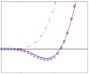
holds true. Figure 3 shows the shear viscosity as a function of granular temperature, (2.27), up to the first order. In the limit of high granular temperature, we recover the result for an inelastic hard-sphere gas while, for a low granular temperature, we find the result for the elastic hard-sphere gas. This agrees with the intuition that, for a high granular temperature, nearly all collisions are dissipative while, for a low granular temperature, elastic collisions dominate. In the intermediate region we obtain a negative overshoot around  $T/T^*\simeq 0.1$. This behaviour is also observed when we assume a Maxwell distribution function (not shown in figure 3). We also show the numerical solution of the differential equation (2.25a,b); details are discussed in Appendix C. The numerical result is consistent with the perturbative solution, that is, the numerics support the validity of the theoretical result.

Figure 3. Shear viscosity as a function of granular temperature obtained from the kinetic theory perturbatively (solid line) and numerically as discussed in Appendix C (open circles) for  $e^*=0.8$, where
  $\eta ^*$ is given by (2.24). The filled squares show results obtained from an event-driven molecular dynamics simulation. The dashed line is the shear viscosity of a hard-sphere gas,
  $\left.\eta ^{(HC)}(e^*)\right / \eta ^{HC}(1)$, (C1). The inset shows a magnification of the intermediate regime.
Similarly, the thermal conductivity and the Dufour-like coefficient  $\mu$ (see Garzó Reference Garzó2019; Shukla, Biswas & Gupta Reference Shukla, Biswas and Gupta2019; Gupta, Shukla & Torrilhon Reference Gupta, Shukla and Torrilhon2020) are, respectively, given by the solutions of the differential equations
 $$\begin{gather} \frac{\partial}{\partial T} \left(4\mu_2 \kappa T^{3/2}\right) + \frac{8}{5}\kappa T^{1/2} \varOmega_\kappa^e {={-}\frac{15}{2} \frac{T}{\sigma^2 }\sqrt{\frac{2}{m}} (1+2a_2),} \end{gather}$$
 $$\begin{gather}-4\mu_2 \frac{\partial \mu}{\partial T}-\frac{8}{5}T^{{-}1}\varOmega_\kappa^e \mu = {\frac{4}{n}\mu_2 \kappa + a_2\frac{15}{2n\sigma^2 } \sqrt{\frac{2T}{m}}.} \end{gather}$$
Introducing new variables
 \begin{equation} \kappa^*\equiv \frac{\kappa}{\kappa^{(HC)}(1)}\quad\text{and}\quad \mu^*=\frac{\dfrac{n\mu}{T}}{\kappa^{(HC)}(1)} \end{equation}
with the thermal conductivity of the elastic hard-sphere gas
 \begin{equation} {\kappa^{(HC)}(1)=\frac{75}{64\sigma^2 }\,\sqrt{\frac{T}{{\rm \pi} m}},} \end{equation}
we can rewrite (2.30) and (2.31),
 $$\begin{gather} 5x \mu_2 \frac{\partial \kappa^*}{\partial x} - \left(10\mu_2-5x \frac{\partial \mu_2}{\partial x} +2\varOmega_\kappa^e\right)\kappa^* =8\sqrt{2{\rm \pi}}(1+2a_2), \end{gather}$$
 $$\begin{gather}10x\mu_2 \frac{\partial \mu^*}{\partial x} -\left(15\mu_2 +4\varOmega_\kappa^e\right) \mu^* =2\mu_2\kappa^* + 16\sqrt{2{\rm \pi}}a_2. \end{gather}$$
Similar to the shear viscosity, we can perturbatively obtain the solutions as
 $$\begin{gather} \kappa^*= \sum_{n=0}^\infty \kappa^{*(n)} = \sum_{n=0}^\infty \left(\frac{5x\mu_2}{10\mu_2-5x\mu_2^\prime+2\varOmega_\kappa^e} \frac{\partial}{\partial x}\right)^n \kappa^{*(0)}, \end{gather}$$
 $$\begin{gather}\mu^*= \sum_{n=0}^\infty \mu^{*(n)} = \sum_{n=0}^\infty \left(\frac{10x\mu_2}{15\mu_2+4\varOmega_\kappa^e} \frac{\partial}{\partial x}\right)^n \mu^{*(0)}, \end{gather}$$
respectively, with
 $$\begin{gather} \mu_2^\prime={\frac{\partial \mu_2}{\partial x}}, \end{gather}$$
 $$\begin{gather}\kappa^{*(0)}={-}\frac{8\sqrt{2{\rm \pi}}(1+2a_2)}{10\mu_2-5x\mu_2^\prime+2\varOmega_\kappa^e}, \end{gather}$$
 $$\begin{gather}\mu^{*(0)}={-}\frac{10\mu_2\kappa^*+16\sqrt{2{\rm \pi}}a_2}{15\mu_2+4\varOmega_\kappa^e}. \end{gather}$$
Figures 4 and 5 show the thermal conductivity, (2.36), and the Dufour-like coefficient  $\mu$, (2.37), as functions of granular temperature. Again, the numerical solution supports the validity of the analytical results.

Figure 4. Thermal conductivity as a function of granular temperature, obtained from the kinetic theory perturbatively (solid line) and numerically as discussed in Appendix C (open circles) for  $e^*=0.8$, where
  $\kappa ^*$ is given by (2.32a,b). The dashed line is the thermal conductivity of a hard-sphere gas
  $\left.\kappa ^{(HC)}(e^*)\right /\kappa ^{(HC)}(1)$ (C 7).

Figure 5. The granular temperature dependence of the Dufour-like coefficient  $\mu$ obtained from the kinetic theory perturbatively (solid line) and numerically as discussed in Appendix C (open circles) for
  $e^*=0.8$, where
  $\mu ^*$ is given by (2.32a,b). The dashed line shows the result for an inelastic hard-sphere gas,
  $n\mu ^{(HC)}(e^*)/(\kappa ^{(HC)}(1)T)$ (C9). The inset shows a magnification of the intermediate regime.
The thermal conductivity has both negative and positive peaks at around  $T/T^*\simeq 0.1$ and
  $0.2$, respectively. Similar to the case of the shear viscosity, these peaks are not found when a Maxwell distribution function is assumed. The Dufour-like coefficient
  $\mu$ behaves similar to the shear viscosity, however, the value becomes negative in this region as shown in the inset of figure 5. This means that the heat flux is directed from dilute regions to dense regions. We will discuss this phenomenon below.
3. Linear stability analysis of the homogeneous cooling state
From the zeroth, first and second moments of the Boltzmann equation, we obtain a set of hydrodynamic equations,
 \begin{equation} \frac{\partial n}{\partial t}+\boldsymbol{\nabla} \boldsymbol{\cdot} (n\boldsymbol{u})=0, \end{equation}
 \begin{equation} \frac{\partial \boldsymbol{u}}{\partial t}+\boldsymbol{u}\boldsymbol{\cdot} \boldsymbol{\nabla} \boldsymbol{u} ={-}\frac{1}{nm}\boldsymbol{\nabla} p+ \frac{\eta}{nm}\left[\nabla^2 \boldsymbol{u}+\frac{1}{3}\boldsymbol{\nabla}(\boldsymbol{\nabla} \boldsymbol{\cdot} \boldsymbol{u})\right], \end{equation}
 \begin{align} \frac{\partial T}{\partial t}+\boldsymbol{u}\boldsymbol{\cdot} \boldsymbol{\nabla} T &={-}\zeta T +\frac{2}{3n}\left(\kappa \nabla^2T + \mu \nabla^2 n\right)-\frac{2}{3n}p (\boldsymbol{\nabla} \boldsymbol{\cdot} \boldsymbol{u})\nonumber\\ &\quad +\frac{2}{3n}\eta \left[(\boldsymbol{\nabla}_\alpha u_\beta)(\boldsymbol{\nabla}_\beta u_\alpha) +(\boldsymbol{\nabla}_\beta u_\alpha)(\boldsymbol{\nabla}_\alpha u_\beta) -\frac{2}{3}(\boldsymbol{\nabla} \boldsymbol{\cdot} \boldsymbol{u})^2\right], \end{align}
with the static pressure  $p=nT$. We linearize the equations around the homogeneous cooling state,
 $$\begin{gather} n(\boldsymbol{r},t) = n_{H}+\delta n, \end{gather}$$
 $$\begin{gather}T(\boldsymbol{r},t) = T_{H}+\delta T, \end{gather}$$
where the subscript  $H$ indicates the quantities due to the homogeneous system and consider only linear terms with respect to
 \begin{equation} \rho \equiv \frac{\delta n}{n_{H}},\quad \boldsymbol{w}\equiv \frac{\boldsymbol{u}}{v_{T}},\quad \theta\equiv \frac{\delta T}{T_{H}},\end{equation}
with the thermal velocity  $v_{T}\equiv \sqrt {2T/m}$. We introduce dimensionless time and space variables,
  $\tau$ and
  $\hat {\boldsymbol {r}}$, by
 $$\begin{gather} \tau \equiv \int_0^t {\rm d}t^\prime \nu_{H}(t^\prime), \end{gather}$$
 $$\begin{gather}\hat{\boldsymbol{r}} \equiv\frac{2\nu_{H}(t)}{v_{T}(t)}\boldsymbol{r}, \end{gather}$$
with the collision frequency for the elastic hard-sphere gas
 \begin{equation} {\nu_{H}= \frac{16}{5} n\sigma^2 \sqrt{\frac{{\rm \pi} T}{m}}. } \end{equation}
After linearization and Fourier transformation, the set of hydrodynamic equations becomes
 $$\begin{gather} \frac{\partial}{\partial \tau}\rho_{k} ={-}{\rm i}k w_{{k}\parallel}, \end{gather}$$
 $$\begin{gather}\frac{\partial}{\partial \tau}w_{{k}\parallel} ={-}\frac{1}{2}{\rm i}k \rho_{k} +\left(\frac{1}{4}\zeta^*-\frac{4}{3}\eta^* k^2\right) w_{\boldsymbol{k}\parallel} -\frac{1}{2}{\rm i}k \theta_{k}, \end{gather}$$
 $$\begin{gather}\frac{\partial}{\partial \tau}w_{{k}\perp} = \left(\frac{1}{4}\zeta^* - \eta^* k^2\right)w_{{k}\perp}, \end{gather}$$
 $$\begin{gather}\frac{\partial}{\partial \tau}\theta_{k} = \left(-\frac{1}{2}\zeta^* -\frac{5}{2}\mu^* k^2\right)\rho_{k} -\frac{2}{3}{\rm i}k w_{{k}\parallel} + \left({-}A\zeta^*-\frac{5}{2}\kappa^* k^2\right)\theta_{k}, \end{gather}$$
with
 \begin{equation} \zeta^*=\zeta \frac{\eta^{(HC)}(1)}{nT} \end{equation}
and
 \begin{equation} A\equiv \frac{1}{4}+\frac{1}{2}T\frac{\partial}{\partial T}\log \mu_2 =\frac{1}{4}-\frac{1}{2}x\frac{\partial}{\partial x}\log \mu_2. \end{equation}
In the limit  $x\to 0$ we obtain
  $A\to 1/4$, which is consistent with the result for hard-sphere gases (Brilliantov & Pöschel Reference Brilliantov and Pöschel2004). The variables
  $\varPsi _{k}(=\rho _{k}, \boldsymbol {w}_{k}, \theta _{k})$ denote the Fourier component of the quantity
  $\varPsi$,
 \begin{equation} \varPsi_{k}(\tau)=\int {\rm d}\,\hat{\boldsymbol{r}} \varPsi(\hat{\boldsymbol{r}},\tau) {\rm e}^{-{\rm i} \boldsymbol{k}\boldsymbol{\cdot} \hat{\boldsymbol{r}}} \end{equation}
and  $w_{\boldsymbol {k}\parallel }$ and
  $\boldsymbol {w}_{\boldsymbol {k}\perp }$ are the longitudinal and transversal components of the velocity field with respect to the dimensionless wave vector
  $\boldsymbol {k}$.
Equation (3.6c) can be easily solved as
 \begin{equation} w_{{k}\perp}(\tau)=w_{{k}\perp}(0) \exp\left(\lambda_\perp \tau\right),\end{equation}
with
 \begin{equation} \lambda_\perp{=} \tfrac{1}{4}\zeta^* - \eta^* k^2, \end{equation}
and the threshold for this shear mode is given by
 \begin{equation} k_\perp{=} \frac{1}{2}\sqrt{\frac{\zeta^*}{\eta^*}}. \end{equation}
 From (3.6a), (3.6b) and (3.6d), the other three eigenmodes  $\lambda _i$ (
 $i=1,2,3$) can be obtained as the solutions of the third-order equation
 \begin{align} &\lambda^3+\left[\left(A-\frac{1}{4}\right)\zeta^*+\left(\frac{4}{3}\eta^*+\frac{5}{2}\kappa^*\right)k^2\right]\lambda^2 \nonumber\\ &\quad +\left[-\frac{1}{4}A\zeta^{*2}+\left(\frac{5}{6}+\frac{4}{3}A\zeta^*\eta^*-\frac{5}{8}\zeta^*\kappa^*\right)k^2 +\frac{10}{3}\eta^*\kappa^* k^4\right]\lambda\nonumber\\ &\quad +\left[\left(\frac{A}{2}-\frac{1}{4}\right)\zeta^*k^2 + \frac{5}{4}(\kappa^*-\mu^*)k^4\right]=0. \end{align}
We can numerically obtain the thresholds for the heat mode and the sound modes from (3.13).
Figure 6 shows the wavenumber dependence of each mode. In the regime of high granular temperature, the real part of the heat mode becomes positive for small  $k$, rendering the heat mode unstable. In contrast, the sound mode is unstable for all
  $k$. For
  $T\simeq 1.6T^*$ and large
  $k$, the real parts of the heat mode are almost equal to those of the sound modes. For a smaller granular temperature, the real part of the heat mode is negative for all
  $k$ and the real parts of the sound modes become positive for small
  $k$, which is not observed for hard-sphere gases. Figure 7 shows the granular temperature dependencies of the threshold values for the shear mode, the heat mode and the sound mode, where
  $k_{h}$ and
  $k_{s}$ are the wavenumbers where (3.13) is satisfied. In the limit of high granular temperature, both thresholds correspond to elastic or dissipative hard-sphere gases. On the other hand, the threshold for the heat mode becomes imaginary below
  $0.5T^*$, while that for the shear mode decreases to zero. Below
  $1.6T^*$, as shown in figure 6, the real part of the heat mode becomes negative while those of the sound modes become positive for small
  $k$. In addition, the threshold for the sound modes has a peak around
  $0.3T^*$.

Figure 6. The wavenumber dependence of the real parts of the heat mode (solid line) and the sound mode (dashed and dotted lines) for  $T/T^*=10$,
  $1.6$, and
  $0.1$ and
  $e^*=0.8$.

Figure 7. Threshold values of the shear mode (solid line), the heat mode (dashed line) and the sound modes (dotted line) as functions of the granular temperature for  $e^*=0.8$. The dotted black line shows the value of the shear mode for a hard-sphere gas. The dot-dashed line refers to the heat mode of a hard-sphere gas. The dashed green line highlights the value
  $T/T^*\approx 0.4$ where the threshold for the heat mode turns imaginary.
We wish to mention that in the limit  $x\to 0$, we obtain
  $A\to \tfrac {1}{4}$ and the structure of (3.11) and (3.13) is consistent with previous results obtained by Garzó (Reference Garzó2005) for hard spheres.
4. Numerical confirmation of the results
In order to validate the theoretical results presented in the preceding sections, we performed event-driven molecular dynamics simulations of the granular system. In particular, here we focus on the numerical measurement of the shear viscosity. Obviously, the shear viscosity in a system operating in the homogeneous cooling state is different from the shear viscosity in a uniformly sheared phase (Santos, Garzó & Dufty Reference Santos, Garzó and Dufty2004; Takada et al. Reference Takada, Saitoh and Hayakawa2016; Takada & Hayakawa Reference Takada and Hayakawa2018). Consequently, we must not determine numerically the value of shear viscosity in the traditional way. Instead, for systems in the homogeneous cooling state, Brey & Cubero (Reference Brey and Cubero2001) introduced a protocol to determine the shear viscosity from a relaxation process, that is, a perturbation is added to the system and the relaxation is observed.
We consider a set of  $N=3000$ particles of mass
  $m$ and diameter
  $\sigma$ homogeneously distributed in a cubic box of side length
  $L=54\,\sigma$ with periodic boundary conditions. The given parameters correspond to a packing fraction of
  $\phi =1.0\times 10^{-2}$ (corresponding to the number density
  $n\sigma ^3\simeq 1.9\times 10^{-2}$). We add a velocity perturbation via
 \begin{equation} u_y(x, t=0) \propto \sin\left(\frac{2{\rm \pi}}{L} x\right) \end{equation}
and observe the relaxation back to the uniform state in the course of time. Following Brey & Cubero (Reference Brey and Cubero2001) and using (3.3a–c) and (3.10), the value of the shear viscosity,  $\eta ^*$, can be obtained from
 \begin{equation} u_y(x, t) \propto \exp(-\eta^* k^2\tau). \end{equation}
Figure 3 (black square symbols) shows the shear viscosity determined by means of (4.2) in comparison with the theoretical results. In the whole range of the granular temperature, the result is consistent with the theory (2.27). Small deviations of the molecular dynamics simulation data from the theory arise due to the statistical nature of the particle system (Brey & Cubero Reference Brey and Cubero2001).
Note that an molecular dynamics numerical confirmation of the thermal conductivity and the Dufour-like coefficient  $\mu$ in a granular system is much more complicated since these two coefficients are coupled (Dufty & Brey Reference Dufty and Brey2002; Brey & Ruiz-Montero Reference Brey and Ruiz-Montero2004; Brey et al. Reference Brey, Ruiz-Montero, Maynar and García de Soria2005).
5. Discussion
To check the validity of the perturbative solution of (2.25a,b) to derive the shear viscosity, we relate the first terms of (2.27) and obtain
 \begin{align} \frac{\eta^{*(1)}}{\eta^{*(0)}}&= \frac{10x\mu_2}{5\mu_2+6\varOmega_\eta^e}\frac{\partial}{\partial x}\log \eta^{*(0)}\nonumber\\ &={-} \frac{10x\mu_2}{(5\mu_2+6\varOmega_\eta^e)^2} \left(5\frac{\partial \mu_2}{\partial x}+6\frac{\partial \varOmega_\eta^e}{\partial x}\right). \end{align}
Figure 8 shows this ratio as a function of the granular temperature for various values of the coefficient of restitution,  $e^*$. Even for moderately large inelasticity, we obtain
  $\eta ^{*(1)}/\eta ^{*(0)} \ll 1$, justifying the perturbation solution.

Figure 8. The ratio  $\eta ^{*(1)}$ to
  $\eta ^{*(0)}$ of the first terms of (2.27) as a function of granular temperature for the restitution coefficient
  $e^*=0.8$ (solid line),
  $e^* =0.5$ (dashed line) and
  $e^* =0.3$ (dotted line).
Let us analyse the crossover behaviour of the viscosity. We define the effective restitution coefficient  $e_{eff}$ (Takada et al. Reference Takada, Serero and Pöschel2017) as
 \begin{equation} 1-e_{eff}^2 = (1-e^{*2})(1+x)e^{{-}x},\end{equation}
where the right-hand side of (5.2) is equivalent to  $S_1$ for
  $\beta v^*\to \infty$ given by (A10a). The hard-sphere limit of
  $a_2$ with this effective restitution coefficient is known to reproduce the peak value of
  $a_2$ in figure 1 (Takada et al. Reference Takada, Serero and Pöschel2017). Let us define the effective shear viscosity as
 \begin{align} \eta_{eff}{= \frac{15}{2(1+e_{eff})(13-e_{eff})\sigma^2 }\sqrt{\frac{mT}{\rm \pi}} \left[1+\frac{3(4-3e_{eff})}{8(13-e_{eff})}a_{2, eff} +\frac{(7-4e_{eff})}{32(13-e_{eff})}a_{3, eff}\right],}\end{align}
with  $a_{2, eff} \equiv a_2^{(HC)}(e_{eff})$ and
  $a_{3, eff} \equiv a_3^{(HC)}(e_{eff})$. Figure 9 represents the granular temperature dependence of the effective shear viscosity (5.3). This simple effective theory (5.2) well reproduces the crossover granular temperature between two regimes.

Figure 9. The granular temperature dependence of the shear viscosity obtained from the kinetic theory up to  $a_3$ order (solid line) and that from the effective theory (dotted line). The dashed line is the shear viscosity of hard-sphere gases
  $\eta ^{(HC)}(e^*)$. The crossover regime (
 $10^{-1}\lesssim T/T^*\lesssim 10^1$) is highlighted in grey.
We also consider the reason for the negativity of the coefficient  $\mu$ in the intermediate granular temperature regime. Upon considering the relaxation dynamics of the hydrodynamic fluxes by mean of a Grad expansion pertaining to granular gases, it was shown by Sela & Goldhirsch (Reference Sela and Goldhirsch1998), Serero et al. (Reference Serero, Noskowicz, Tan and Goldhirsch2009) and Serero (Reference Serero2009) that the origin of the contribution to the heat flux proportional to the gradient of the density could be traced back to the time dependence in granular gases of the microscopic time scale (the means free time). In the case of the heat flux, this dependence manifests itself through the emergence in the post-relaxation expression of the heat flux of a gradient of the cooling coefficient (Serero et al. Reference Serero, Noskowicz, Tan and Goldhirsch2009; Serero Reference Serero2009) (expressing the difference in the dynamics of the granular temperature on the sub-resolved scale), giving rise to a gradient of the density (see Serero (Reference Serero2009) and Serero et al. (Reference Serero, Noskowicz, Tan and Goldhirsch2009) for a detailed derivation in the case of a monodisperse and bidisperse system of inelastic hard spheres, respectively). In the present case, this mechanism can yield a negative
  $\mu$ coefficient when combined with the particular form of the distribution function at hand, as detailed below. Note that this cannot be observed when we only use the Maxwell distribution function to determine the coefficient
  $\mu$ as shown in figure 10, which means that the origin of the negativeness comes from the deviation of the distribution function from the Gaussian. Let us consider two regions, one of which is slightly denser (system I) and the other is diluter (system II) with the same granular temperature around
  $T/T^*\simeq 0.1$. Although the distribution function is the same, the number of particles is different. Because the number of particles whose velocity is higher than
  $v^*$ in system I is larger, the number of inelastic collisions increases, and the granular temperature of the former decays slightly faster than that of the latter. As a result, the granular temperature in system I is slightly smaller than that in system II (
 $T_{I} \lesssim T_{II}$), and this yields
  $a_2(T_{I})\gtrsim a_2(T_{II})$. In addition, as our previous paper (Takada et al. Reference Takada, Serero and Pöschel2017) reported, the population of the particles having
  $1\lesssim v/v_{T}\lesssim 2$ and
  $v/v_{T}\gtrsim 2$ in system I are higher and lower than those in system II, respectively (in this case,
  $v_{T}\simeq 0.3 v^*$). Therefore, the heat flux goes from system II to system I, because the number of particles having higher velocities is larger in system II. This is the reason for the negative overshoot of
  $\mu$ in the intermediate granular temperature regime. It is noted that the transient behaviour of the thermal conductivity is similarly explained. Note that the effect of a negative coefficient
  $\mu$ was also reported for driven granular gases by González & Garzó (Reference González and Garzó2019) and for confined quasi-two-dimensional granular gases by Brey et al. (Reference Brey, Buzón, Maynar and García de Soria2015) and Garzó, Brito & Soto (Reference Garzó, Brito and Soto2018).

Figure 10. The granular temperature dependence of the coefficient  $\mu$ obtained from the kinetic theory up to
  $a_3$ order (solid line), that up to
  $a_2$ order (open circles) and that determined from the Maxwell distribution function (dot-dashed line) for
  $e^*=0.8$.
6. Conclusion
In this paper we have derived the granular temperature dependence of the transport coefficients for charged granular gases in the discontinuous limit of the effective restitution coefficient. The negative overshoots of the transport coefficients appear because of the non-Gaussianity of the distribution function. Especially, we have found that the coefficient  $\mu$ becomes negative in the intermediate granular temperature regime. We have also performed the linear stability analysis for the homogeneous cooling state, which shows that the stability of the thermal and sound modes become reversal in the low granular temperature regime, and this threshold is about
  $0.5T^*$. We have also performed the molecular dynamics simulation and we have obtained a consistent result with that from the kinetic theory.
Acknowledgements
S.T. wishes to express his sincere gratitude to the Yukawa Institute for Theoretical Physics for financial support towards his research visit at Friedrich-Alexander-Universität Erlangen-Nürnberg. Numerical computation in this work was partially carried out at the Yukawa Institute Computer Facility. We thank the Interdisciplinary Center for Nanostructured Films (IZNF), the Central Institute for Scientific Computing (ZISC) and the Interdisciplinary Center for Functional Particle Systems (FPS) at Friedrich-Alexander University Erlangen-Nürnberg.
Funding
This work was supported by Kompetenznetzwerk für wissenschaftliches Höchstleistungsrechnen in Bayern (KONWIHR) Satoshi Takada is partially supported by Scientific Grant-in-Aid of Japan Society for the Promotion of Science, KAKENHI (grants nos. 20K14428 and 21H01006).
Declaration of interests
The authors report no conflict of interest.
Appendix A. Computation of the Sonine coefficients  $a_2$ and $a_3$ from the Boltzmann equation


We expand the distribution function in Sonine polynomials up to third order,  $a_3$; see (2.4). Then, we rewrite the expression of the
  $p$th moment of the collision integral in the form
 \begin{align} \mu_p &={-}\tfrac{1}{2}\int {\rm d}\boldsymbol{C} \,{\rm d}\boldsymbol{c}_{12} \,{\rm d}\hat{\boldsymbol{k}} \, \varTheta(\boldsymbol{c}_{12}\boldsymbol{\cdot} \hat{\boldsymbol{k}})\left|\boldsymbol{c}_{12}\boldsymbol{\cdot} \hat{\boldsymbol{k}}\right|\phi(c_1)\phi(c_2) \nonumber\\ &\quad \times \big\{1+a_2 \big[S_2(c_1^2)+S_2(c_2^2)\big] + a_3 \big[S_3(c_1^2)+S_3(c_2^2)\big]\big\} \varDelta (c_1^p+c_2^p), \end{align}
where we have neglected the terms proportional to  $a_2^2$,
  $a_3^2$ and
  $a_2a_3$. The product of the dimensionless distribution function is then
 \begin{align} &1+a_2 \big[S_2(c_1^2)+S_2(c_2^2)\big] + a_3 \big[S_3(c_1^2)+S_3(c_2^2)\big]\nonumber\\ &\quad = 1+a_2 \left[ C^4+\tfrac{1}{2}C^2c_{12}^2-5C^2+\tfrac{1}{16}c_{12}^4-\tfrac{5}{4}c_{12}^2+( \boldsymbol{C}\boldsymbol{\cdot} \boldsymbol{c}_{12})^2 +\tfrac{15}{4} \right]\nonumber\\ &\qquad +a_3\left[ -\tfrac{1}{3}C^6 - \tfrac{1}{4}C^4c_{12}^2+\tfrac{7}{2}C^4- \tfrac{1}{16}C^2c_{12}^4+\tfrac{7}{4}C^2c_{12}^2 -C^2(\boldsymbol{C}\boldsymbol{\cdot} \boldsymbol{c}_{12})^2 -\tfrac{35}{4}C^2\right.\nonumber\\ &\qquad \left.-\tfrac{1}{192}c_{12}^6+\tfrac{7}{32}c_{12}^4-\tfrac{1}{4}c_{12}^2(\boldsymbol{C}\boldsymbol{\cdot} \boldsymbol{c}_{12})^2-\tfrac{35}{16}c_{12}^2+\tfrac{7}{2}(\boldsymbol{C}\boldsymbol{\cdot} \boldsymbol{c}_{12})^2 + \tfrac{35}{8} \right], \end{align}
and the terms  $\varDelta (c_1^p+c_2^p)$ for
  $p=2$,
  $4$ and
  $6$ are, respectively, given by
 \begin{align} \varDelta (c_1^2+c_2^2) &={-}\frac{1-e^2}{2}(\boldsymbol{c}_{12}\cdot \hat{\boldsymbol{k}})^2,\end{align}
 \begin{align} \varDelta (c_1^4+c_2^4)&={-}(1-e^2)C^2(\boldsymbol{c}_{12}\boldsymbol{\cdot} \hat{\boldsymbol{k}})^2-\frac{1}{4}(1-e^2)c_{12}^2(\boldsymbol{c}_{12}\boldsymbol{\cdot} \hat{\boldsymbol{k}})^2\nonumber\\ &\quad -4(1+e)(\boldsymbol{C}\boldsymbol{\cdot} \boldsymbol{c}_{12})(\boldsymbol{C} \boldsymbol{\cdot} \hat{\boldsymbol{k}})(\boldsymbol{c}_{12}\boldsymbol{\cdot}\hat{\boldsymbol{k}})\nonumber\\ &\quad +2(1+e)^2(\boldsymbol{C}\boldsymbol{\cdot}\hat{\boldsymbol{k}})^2(\boldsymbol{c}_{12}\boldsymbol{\cdot} \hat{\boldsymbol{k}})^2 +\frac{(1-e^2)^2}{8}(\boldsymbol{c}_{12}\boldsymbol{\cdot} \hat{\boldsymbol{k}})^4, \end{align}
 \begin{align} \varDelta (c_1^6+c_2^6)&={-}\frac{3(1-e^2)}{2}C^4(\boldsymbol{c}_{12}\boldsymbol{\cdot} \hat{\boldsymbol{k}})^2 -\frac{3(1-e^2)}{4}C^2c_{12}^2 (\boldsymbol{c}_{12}\boldsymbol{\cdot} \hat{\boldsymbol{k}})^2\nonumber\\ &\quad -12(1+e)C^2(\boldsymbol{C}\boldsymbol{\cdot} \boldsymbol{c}_{12}) (\boldsymbol{C}\boldsymbol{\cdot} \hat{\boldsymbol{k}})(\boldsymbol{c}_{12}\boldsymbol{\cdot} \hat{\boldsymbol{k}}) +6(1+e)^2C^2 (\boldsymbol{C}\boldsymbol{\cdot} \hat{\boldsymbol{k}})^2(\boldsymbol{c}_{12} \boldsymbol{\cdot} \hat{\boldsymbol{k}})^2\nonumber\\ &\quad+\frac{3(1-e^2)^2}{8}C^2(\boldsymbol{c}_{12}\boldsymbol{\cdot} \hat{\boldsymbol{k}})^4 -\frac{3(1-e^2)}{32}c_{12}^4 (\boldsymbol{c}_{12}\boldsymbol{\cdot} \hat{\boldsymbol{k}})^2\nonumber\\ &\quad -3(1+e)c_{12}^2(\boldsymbol{C}\boldsymbol{\cdot} \boldsymbol{c}_{12}) (\boldsymbol{C}\boldsymbol{\cdot} \hat{\boldsymbol{k}})(\boldsymbol{c}_{12}\boldsymbol{\cdot} \hat{\boldsymbol{k}}) +\frac{3(1+e)^2}{2} c_{12}^2(\boldsymbol{C}\boldsymbol{\cdot} \hat{\boldsymbol{k}})^2(\boldsymbol{c}_{12} \boldsymbol{\cdot} \hat{\boldsymbol{k}})^2\nonumber\\ &\quad +\frac{3(1-e^2)^2}{32} c_{12}^2 (\boldsymbol{c}_{12}\boldsymbol{\cdot} \hat{\boldsymbol{k}})^4 -\frac{3(1-e^2)}{2}(\boldsymbol{C}\boldsymbol{\cdot} \boldsymbol{c}_{12})^2 (\boldsymbol{c}_{12}\boldsymbol{\cdot} \hat{\boldsymbol{k}})^2\nonumber\\ &\quad +3(1+e)(1-e^2)(\boldsymbol{C}\boldsymbol{\cdot} \boldsymbol{c}_{12}) (\boldsymbol{C}\boldsymbol{\cdot} \hat{\boldsymbol{k}})(\boldsymbol{c}_{12} \boldsymbol{\cdot} \hat{\boldsymbol{k}})^3\nonumber\\ &\quad -\frac{3(1+e)^2(1-e^2)}{2} (\boldsymbol{C}\boldsymbol{\cdot} \hat{\boldsymbol{k}})^2(\boldsymbol{c}_{12}\boldsymbol{\cdot} \hat{\boldsymbol{k}})^4 -\frac{(1-e^2)^3}{32}(\boldsymbol{c}_{12}\boldsymbol{\cdot} \hat{\boldsymbol{k}})^6. \end{align}
Using (A2)–(A3c), we can calculate  $\mu _p$ for
  $p=2$,
  $4$ and
  $6$ from (A1) as
 $$\begin{gather} \mu_2 = \sqrt{2{\rm \pi}}(S_1+a_2 S_2 + a_3S_3), \end{gather}$$
 $$\begin{gather}\mu_4 = \sqrt{2{\rm \pi}}(T_1+a_2 T_2 + a_3T_3), \end{gather}$$
 $$\begin{gather}\mu_6 = \sqrt{2{\rm \pi}}(D_1+a_2 D_2 + a_3D_3), \end{gather}$$
with
 \begin{gather} S_1= \tfrac{1}{2}\int_0^\infty {\rm d}c_{12} \int_0^1 {\rm d}(\cos\theta) (1-e^2)\cos^3\theta c_{12}^5 \exp\left(-\tfrac{1}{2}c_{12}^2\right),\end{gather}
 \begin{gather} S_2= \tfrac{1}{32}\int_0^\infty {\rm d}c_{12} \int_0^1 {\rm d}(\cos\theta) (1-e^2) \cos^3\theta c_{12}^5 (15-10c_{12}^2+c_{12}^4) \exp\left(-\tfrac{1}{2}c_{12}^2\right),\end{gather}
 \begin{align} S_3&= \tfrac{1}{384}\int_0^\infty {\rm d}c_{12} \int_0^1 {\rm d}(\cos\theta) (1-e^2) \cos^3\theta c_{12}^5 \nonumber\\ &\quad \times (105-105c_{12}^2+21c_{12}^4-c_{12}^6) \exp\left(-\tfrac{1}{2}c_{12}^2\right), \end{align}
 \begin{align} T_1 &= \tfrac{1}{8}\int_0^\infty {\rm d}c_{12} \int_0^1 {\rm d}(\cos\theta) (1-e^2) \cos^3\theta c_{12}^5\nonumber\\ &\quad \times \big[10+2c_{12}^2 - (1-e^2)\cos^2\theta c_{12}^2\big] \exp\left(-\tfrac{1}{2}c_{12}^2\right), \end{align}
 \begin{align} T_2&= \tfrac{1}{2}\int_0^\infty {\rm d}c_{12} \int_0^1 {\rm d}(\cos\theta) (1+e) \cos^3\theta c_{12}^5 \exp\left(-\tfrac{1}{2}c_{12}^2\right)\nonumber\\ &\quad +\tfrac{1}{128}\int_0^\infty {\rm d}c_{12} \int_0^1 {\rm d}(\cos\theta) (1-e^ 2) \cos^3\theta c_{12}^5 \exp\left(-\tfrac{1}{2}c_{12}^2\right)\nonumber\\ &\quad \times \big[ 2({-}25-7c_{12}^2-5c_{12}^4+c_{12}^6) + \cos^2\theta c_{12}^2(17+10c_{12}^2-c_{12}^4)\nonumber\\ &\quad +e^2\cos^2\theta c_{12}^2 (15-10c_{12}^2+c_{12}^4) \big], \end{align}
 \begin{align} T_3&= \tfrac{1}{8} \int_0^\infty {\rm d}c_{12} \int_0^1 {\rm d}(\cos\theta) (1+e) \cos^3\theta (1-\cos^2\theta) c_{12}^7(7-c_{12}^2)\exp\left(-\tfrac{1}{2}c_{12}^2\right)\nonumber\\ &\quad+\tfrac{1}{1536} \int_0^\infty {\rm d}c_{12} \int_0^1 {\rm d}(\cos\theta) (1-e^2) \cos^3\theta c_{12}^5 \exp\left(-\tfrac{1}{2}c_{12}^2\right) \nonumber\\ &\quad \times \big[ 2({-}525+168c_{12}^2\,{-}\,54c_{12}^4+16c_{12}^6-c_{12}^8) + \cos^2\theta c_{12}^2(567+9c_{12}^2\,{-}\,21c_{12}^4+c_{12}^6) \nonumber\\ &\quad +e^2\cos^2\theta c_{12}^2 (105-105c_{12}^2+21c_{12}^4-c_{12}^6) \big], \end{align}
 \begin{align} D_1&= \tfrac{1}{32}\int_0^\infty {\rm d}c_{12} \int_0^1 {\rm d}(\cos\theta) (1-e^2) \cos^3\theta c_{12}^5 \exp\left(-\tfrac{1}{2}c_{12}^2\right)\nonumber\\ &\quad \times \big[3(35+14c_{12}^2+c_{12}^4) -3(1-e^2)\cos^2\theta c_{12}^2 (7+c_{12}^2) + (1-e^2)^2 \cos^4\theta c_{12}^4\big], \end{align}
 \begin{align} D_2&= \tfrac{3}{16} \int_0^\infty {\rm d}c_{12} \int_0^1 {\rm d}(\cos\theta) (1+e) \cos^3\theta c_{12}^7\nonumber\\ &\quad \times \big[2-(1+e)\cos^2\theta\big] \big[7+c_{12}^2-(1-e^2)\cos^2\theta c_{12}^2\big] \exp\left(-\tfrac{1}{2}c_{12}^2\right)\nonumber\\ &\quad +\tfrac{1}{512} \int_0^\infty {\rm d}c_{12} \int_0^1 {\rm d}(\cos\theta) (1-e^2) \cos^3\theta c_{12}^5 \exp\left(-\tfrac{1}{2}c_{12}^2\right)\nonumber\\ &\quad \times \big[ 3({-}595-28c_{12}^2+14c_{12}^4+4c_{12}^6+c_{12}^8)\nonumber\\ &\quad +3(1-e^2)\cos^2\theta c_{12}^2(35+19c_{12}^2+3c_{12}^4-c_{12}^6) \nonumber\\ &\quad + (1-e^2)^2 \cos^4\theta c_{12}^4 (15-10c_{12}^2+c_{12}^4)\big], \end{align}
 \begin{align} D_3&= \tfrac{3}{64} \int_0^\infty {\rm d}c_{12} \int_0^1 {\rm d}(\cos\theta) (1+e) \cos^3\theta c_{12}^7 \exp\left(-\tfrac{1}{2}c_{12}^2\right)\nonumber\\ &\quad\times \big[2-(1+e)\cos^2\theta\big] \big[35-c_{12}^4-(1-e^2)\cos^2\theta c_{12}^2(7-c_{12}^2)\big]\nonumber\\ &\quad + \tfrac{1}{6144} \int_0^\infty {\rm d}c_{12} \int_0^1 {\rm d}(\cos\theta) (1-e^2) \cos^3\theta c_{12}^5 \exp\left(-\tfrac{1}{2}c_{12}^2\right)\nonumber\\ &\quad \times\big[3({-}5145+1575c_{12}^2+798c_{12}^4-74c_{12}^6+7c_{12}^8-c_{12}^{10})\nonumber\\ &\quad +3(1-e^2)\cos^2\theta c_{12}^2 (735-126c_{12}^2+24c_{12}^4-14c_{12}^6+c_{12}^8) \nonumber\\ &\quad +(1-e^2)^2\cos^4\theta c_{12}^4 (105-105c_{12}^2+21c_{12}^4-c_{12}^6)\big]. \end{align}
Here, we use the relations between the moments  $\mu _p$ of different order,
 $$\begin{gather} \mu_4 = 5\mu_2(1+2a_2), \end{gather}$$
 $$\begin{gather}\mu_6 = \tfrac{105}{4}\mu_2 (1+3a_2-a_3). \end{gather}$$
Substituting (A4) into (A8), we obtain
 $$\begin{gather} (5S_1+5S_2-T_2)a_2 + (5S_3-T_3)a_3=T_1-5S_1, \end{gather}$$
 $$\begin{gather}\left(\tfrac{315}{4}S_1+\tfrac{105}{4}S_2-D_2\right)a_2 + \left(-\tfrac{105}{4}S_1+\tfrac{105}{4}S_3-D_3\right)a_3 = D_1-\tfrac{105}{4}S_1. \end{gather}$$
Using (A9), we obtain the coefficients  $a_2$ and
  $a_3$ in the form given by (2.9a,b).
In the discontinuous limit,  $\beta v^*\to \infty$, (A5a)–(A7c) read as
 $$\begin{gather} {S_1^{(\infty)}(x)}= \left(1-e^{*2}\right) (1+x)e^{{-}x}, \end{gather}$$
 $$\begin{gather}{S_2^{(\infty)}(x)}= \frac{3}{16}\left(1-e^{*2}\right) \left(1+x+\frac{x^2}{3}\right) e^{{-}x}, \end{gather}$$
 $$\begin{gather}{S_3^{(\infty)}(x)}=\tfrac{1}{64}\left(1-e^{*2}\right)\left(1+x-2x^2+\tfrac{28}{3}x^3-\tfrac{8}{3}x^4\right)e^{{-}x}, \end{gather}$$
 \begin{align} {T_1^{(\infty)}(x)} &= \left(1-e^{*2}\right) \left[\frac{9}{2} \left(1+x+\frac{x^2}{9}\right) +e^{*2} \left(1+x+\frac{x^2}{2}\right)\right] e^{{-}x}, \end{align}
 \begin{align} {T_2^{(\infty)}(x)}&= \frac{3}{32}\left(1-e^{*2}\right) \left[69 \left(1+x + \frac{119x^2}{207} +\frac{32x^3}{207} + \frac{4x^4}{207}\right)\right.\nonumber\\ &\quad \left. +10e^{*2} \left(1+x + \frac{x^2}{2} +\frac{2x^3}{15} + \frac{2x^4}{15}\right)\right] e^{{-}x}\nonumber\\ &\quad -2\left(1-e^*\right)(1+x)e^{{-}x}+4, \end{align}
 \begin{align} {T_3^{(\infty)}(x)}&={-}\frac{1}{128}(1-e^{*2})\left[ 117\left( 1+x+\frac{19}{117}x^2+\frac{10}{13}x^3+\frac{4}{39}x^4+\frac{8}{351}x^5 \right)\right.\nonumber\\ &\quad \left. +10e^{*2}\left(1+x+\frac{x^2}{2}+\frac{x^3}{3}-\frac{2x^4}{3}+\frac{4x^5}{15}\right) \right]e^{{-}x} \nonumber\\ &\quad +\frac{1}{2}(1-e^*)(1+x+2x^2)e^{{-}x}-1, \end{align}
 \begin{align} {D_1^{(\infty)}(x)}&= \frac{3}{16}(1-e^{*2})\left[115\left(1+x+\frac{22x^2}{115}+\frac{4x^3}{345}\right) +44e^{*2}\left(1+x+\frac{x^2}{2}+\frac{x^3}{33}\right)\right.\nonumber\\ &\quad \left. +8e^{*4}\left(1+x+\frac{x^2}{2}+\frac{x^3}{6}\right)\right]e^{{-}x}, \end{align}
 \begin{align} {D_2^{(\infty)}(x)} &= \frac{3}{256}(1-e^{*2})\left[ 5737\left(1+x+\frac{2850x^2}{5737}+\frac{2120x^3}{17\,211}+\frac{248x^4}{17\,211}+\frac{16x^5}{17\,211}\right) \right.\nonumber\\ &\quad \left.+1572e^{*2}\left(1+x+\frac{x^2}{2}+\frac{221x^3}{1179}+\frac{62x^4}{1179}+\frac{4x^5}{1179}\right)\right.\nonumber\\ &\quad \left. +280e^{*4}\left(1+x+\frac{x^2}{2}+\frac{x^3}{6}+\frac{4x^4}{105}+\frac{2x^5}{105}\right)\right]e^{{-}x}\nonumber\\ &\quad +\frac{3}{2}(1+e^*)\left[ 20\left(1+x+\frac{9x^2}{40}\right) -9e^*\left(1+x+\frac{x^2}{2}\right) \right.\nonumber\\ &\quad \left. +10e^{*2}\left(1+x+\frac{x^2}{2}+\frac{x^3}{10}\right) - 6e^{*3}\left(1+x+\frac{x^2}{2}+\frac{x^3}{6}\right)\right] e^{{-}x}\nonumber\\ &\quad-45\left(1+x+\frac{2x^2}{15}\right) e^{{-}x}+45, \end{align}
 \begin{align} {D_3^{(\infty)}(x)}&={-}\frac{3}{1024}(1-e^{*2})\left[9161\left(1+x+\frac{4528x^2}{9161}+\frac{2132x^3}{9161}+\frac{1640x^4}{27\,483}\right.\right.\nonumber\\ &\quad \left.\left.+\frac{128x^5}{27\,483}+\frac{32x^6}{27\,483}\right)\right.\nonumber\\ &\quad \left.+1636e^{*2}\left(1+x+\frac{x^2}{2}+\frac{140x^3}{1227}+\frac{76x^4}{1227}+\frac{32x^5}{1227}+\frac{8x^6}{3681}\right)\right.\nonumber\\ &\quad \left. +280e^{*4}\left(1+x+\frac{x^2}{2}+\frac{x^3}{6}+\frac{x^4}{21}-\frac{2x^5}{105}+\frac{4x^6}{315}\right)\right]e^{{-}x}\nonumber\\ &\quad -\frac{9}{8}(1+e^*)\left[ 20\left(1+x+\frac{71x^2}{120}+\frac{3x^3}{20}\right) -9e^*\left(1+x+\frac{x^2}{2}+\frac{x^3}{3}\right)\right.\nonumber\\ &\quad \left. + 10e^{*2}\left(1+x+\frac{x^2}{2}+\frac{7x^3}{30}+\frac{x^4}{15}\right)\right.\nonumber\\ &\quad \left. -6e^{*3}\left(1+x+\frac{x^2}{2}+\frac{x^3}{6}+\frac{x^4}{9}\right)\right]e^{{-}x}\nonumber\\ &\quad +\frac{135}{4}\left(1+x+\frac{28x^2}{45}+\frac{4x^3}{45}\right)e^{{-}x}-\frac{135}{4}. \end{align}
It can be shown that in the limit  $x\to 0$, the above expressions are identical to the corresponding expressions for a hard-sphere gas (Brilliantov & Pöschel Reference Brilliantov and Pöschel2006; Santos & Montanero Reference Santos and Montanero2009; Chamorro et al. Reference Chamorro, Reyes and Garzó2013). Using (A9), we can also obtain explicit expressions for
  $a_2$ and
  $a_3$. These expressions are rather cumbersome and not shown here.
Appendix B. Calculation of $\varOmega _\eta ^e$ and $\varOmega _\kappa ^e$ given by (2.11) and (2.14)


Using the definition of  $\tilde {D}_{\alpha \beta }(\boldsymbol {c})$, (2.12), we obtain
 \begin{align} &\tilde{D}_{\alpha\beta}(\boldsymbol{c}_2) \varDelta [\tilde{D}_{\alpha\beta}(\boldsymbol{c}_1)+\tilde{D}_{\alpha\beta}(\boldsymbol{c}_2)]\nonumber\\ &\quad =\left(c_{2i}c_{2j}-\frac{1}{3}\delta_{ij}c_2^2\right) \left[ c_{1i}^\prime c_{1j}^\prime + c_{2i}^\prime c_{2j}^\prime -c_{1i} c_{1j} - c_{2i} c_{2j} -\frac{1}{3}\delta_{ij}\left(c_1^{\prime2}+c_2^{\prime2}-c_1^2-c_2^2\right)\right]\nonumber\\ &\quad=\frac{1-e^2}{6}C^2(\boldsymbol{c}_{12}\boldsymbol{\cdot} \hat{\boldsymbol{k}})^2 + \frac{1+e}{2}c_{12}^2 (\boldsymbol{C} \boldsymbol{\cdot} \hat{\boldsymbol{k}})(\boldsymbol{c}_{12}\boldsymbol{\cdot} \hat{\boldsymbol{k}}) -\frac{(1+e)(5+e)}{24} c_{12}^2 (\boldsymbol{c}_{12}\boldsymbol{\cdot} \hat{\boldsymbol{k}})^2\nonumber\\ &\qquad - (1+e)(\boldsymbol{C}\boldsymbol{\cdot} \boldsymbol{c}_{12})(\boldsymbol{C}\boldsymbol{\cdot} \hat{\boldsymbol{k}})(\boldsymbol{c}_{12} \boldsymbol{\cdot} \hat{\boldsymbol{k}}) +\frac{(1+e)(2+e)}{6}(\boldsymbol{C}\boldsymbol{\cdot} \boldsymbol{c}_{12})(\boldsymbol{c}_{12}\boldsymbol{\cdot} \hat{\boldsymbol{k}})^2\nonumber\\ &\qquad +\frac{(1+e)^2}{2}(\boldsymbol{C}\boldsymbol{\cdot} \hat{\boldsymbol{k}})^2(\boldsymbol{c}_{12}\boldsymbol{\cdot} \hat{\boldsymbol{k}})^2 -\frac{(1+e)^2}{2} (\boldsymbol{C}\boldsymbol{\cdot} \hat{\boldsymbol{k}})(\boldsymbol{c}_{12}\boldsymbol{\cdot} \hat{\boldsymbol{k}})^3 +\frac{(1+e)^2}{8}(\boldsymbol{c}_{12}\boldsymbol{\cdot} \hat{\boldsymbol{k}})^4. \end{align}
We also use the expressions of the Sonine expansion as
 \begin{align} &1+a_2 S_2(c_1)^2+a_3 S_3(c_1^2)\nonumber\\ &\quad =1+a_2 \left[\tfrac{1}{2}C^4+\tfrac{1}{4}C^2c_{12}^2+C^2(\boldsymbol{C}\boldsymbol{\cdot} \boldsymbol{c}_{12}) -\tfrac{5}{2}C^2+\tfrac{1}{32}c_{12}^4\right.\nonumber\\ &\qquad \left. +\tfrac{1}{4}c_{12}^2(\boldsymbol{C}\boldsymbol{\cdot} \boldsymbol{c}_{12}) -\tfrac{5}{8}c_{12}^2+ \tfrac{1}{2}(\boldsymbol{C}\boldsymbol{\cdot} \boldsymbol{c}_{12})^2 -\tfrac{5}{2}(\boldsymbol{C}\boldsymbol{\cdot} \boldsymbol{c}_{12})+\tfrac{15}{8}\right]\nonumber\\ &\qquad +a_3 \left[ -\tfrac{1}{6}C^6 -\tfrac{1}{8}C^4c_{12}^2 -\tfrac{1}{2}C^4(\boldsymbol{C}\boldsymbol{\cdot} \boldsymbol{c}_{12}) +\tfrac{7}{4}C^4 -\tfrac{1}{32}C^2c_{12}^4 -\tfrac{1}{4}C^2c_{12}^2(\boldsymbol{C}\boldsymbol{\cdot} \boldsymbol{c}_{12}) \right.\nonumber\\ &\qquad +\tfrac{7}{8}C^2c_{12}^2 -\tfrac{1}{2}C^2(\boldsymbol{C}\boldsymbol{\cdot} \boldsymbol{c}_{12})^2 +\tfrac{7}{2}C^2(\boldsymbol{C}\boldsymbol{\cdot} \boldsymbol{c}_{12}) -\tfrac{35}{8}C^2 -\tfrac{1}{384}c_{12}^6\nonumber\\ &\qquad -\tfrac{1}{32}c_{12}^4(\boldsymbol{C}\boldsymbol{\cdot} \boldsymbol{c}_{12}) +\tfrac{7}{64}c_{12}^4 -\tfrac{1}{8}c_{12}^2(\boldsymbol{C}\boldsymbol{\cdot} \boldsymbol{c}_{12})^2 +\tfrac{7}{8}c_{12}^2(\boldsymbol{C}\boldsymbol{\cdot} \boldsymbol{c}_{12}) \nonumber\\ &\qquad \left. -\tfrac{35}{32}c_{12}^2 -\tfrac{1}{6}(\boldsymbol{C}\boldsymbol{\cdot} \boldsymbol{c}_{12})^3 +\tfrac{7}{4}(\boldsymbol{C}\boldsymbol{\cdot} \boldsymbol{c}_{12})^2 -\tfrac{35}{8}(\boldsymbol{C}\boldsymbol{\cdot} \boldsymbol{c}_{12}) +\tfrac{35}{16}\right]. \end{align}
Substituting (B1) and (B2) into (2.11), we obtain
 \begin{equation} \varOmega_\eta^e \equiv \sqrt{2{\rm \pi}}\left(\omega_{\eta,1}^e + a_2 \omega_{\eta,2}^e+a_3\omega_{\eta,3}^e\right), \end{equation}
with
 \begin{align} \omega_{\eta,1}^e &={-}\tfrac{1}{12} \int_0^\infty {\rm d}c_{12} \int_0^1 {\rm d}(\cos\theta) (1+e)\big[5+e-3(1+e)\cos^2\theta\big]\nonumber\\ &\quad \times\cos^3\theta c_{12}^7 \exp\left(-\tfrac{1}{2}c_{12}^2\right), \end{align}
 \begin{align} \omega_{\eta,2}^e &={-}\tfrac{1}{384} \int_0^\infty {\rm d}c_{12} \int_0^1 {\rm d}(\cos\theta) (1+e) \big[5+e-3(1+e)\cos^2\theta\big]\nonumber\\ &\quad \times \cos^3\theta c_{12}^7 (63-18c_{12}^2+c_{12}^4) \exp\left(-\tfrac{1}{2}c_{12}^2\right), \end{align}
 \begin{align} \omega_{\eta,3}^e&={-}\tfrac{1}{4608}\int_0^\infty {\rm d}c_{12} \int_0^1 {\rm d}(\cos\theta) (1+e) \big[5+e-3(1+e)\cos^2\theta\big]\nonumber\\ &\quad \times \cos^3\theta c_{12}^7 (693-297c_{12}^2+33c_{12}^4-c_{12}^6) \exp\left(-\tfrac{1}{2}c_{12}^2\right). \end{align}
For  $\beta v^*\to \infty$, these quantities reduce to
 \begin{align} \omega_{\eta,1}^{e(\infty)} &={-}4+(1-e^*)\big[(1-e^*)(1+x)-\tfrac{2}{3}(1+e^*)x^2\big]e^{{-}x}, \end{align}
 \begin{align} \omega_{\eta,2}^{e(\infty)} &=\tfrac{1}{8}-\tfrac{1}{32}(1-e^*)\big[(1-e^*)(1+x)+6(9+e^*)x^2\nonumber\\ &\quad -4(13+7e^*) x^3+8(1+e^*)x^4\big]e^{{-}x}, \end{align}
 \begin{align} \omega_{\eta,3}^{e(\infty)} &=\tfrac{1}{32}-\tfrac{1}{128}(1-e^*)\left[(1-e^*)(1+x)+\tfrac{4}{3}(31+4e^*)x^2-\tfrac{8}{3}(24+11e^*)x^3\right.\nonumber\\ &\quad \left.+\tfrac{16}{3}(4+3e^*)x^4-\tfrac{16}{9}(1+e^*)x^5\right]e^{{-}x}. \end{align}
 In a similar way, we derive  $\varOmega _\kappa ^e$ defined by (2.14). Using the definition of
  $\tilde {\boldsymbol {S}}(\boldsymbol {c})$, (2.15), we write
 \begin{align}
&\tilde{\boldsymbol{S}}(\boldsymbol{c}_2)\boldsymbol{\cdot}
\varDelta
\left[\tilde{\boldsymbol{S}}(\boldsymbol{c}_1)+\tilde{\boldsymbol{S}}(\boldsymbol{c}_2)\right]\nonumber\\
&\quad =\left(c_2^2-\frac{5}{2}\right)\left[
(\boldsymbol{c}_1^\prime \boldsymbol{\cdot}
\boldsymbol{c}_2)c_1^{\prime2}+(\boldsymbol{c}_2^\prime
\boldsymbol{\cdot} \boldsymbol{c}_2)c_2^{\prime2}
-(\boldsymbol{c}_1 \boldsymbol{\cdot}
\boldsymbol{c}_2)c_1^2-(\boldsymbol{c}_2 \boldsymbol{\cdot}
\boldsymbol{c}_2)c_2^2 \right]\nonumber\\
&\quad={-}\frac{1-e^2}{2}C^4(\boldsymbol{c}_{12}\boldsymbol{\cdot}
\hat{\boldsymbol{k}})^2
+\frac{1+e}{2}C^2c_{12}^2(\boldsymbol{C}\boldsymbol{\cdot}
\hat{\boldsymbol{k}})(\boldsymbol{c}_{12}\boldsymbol{\cdot}
\hat{\boldsymbol{k}})
-\frac{1-e^2}{8}C^2c_{12}^2(\boldsymbol{c}_{12}\boldsymbol{\cdot}
\hat{\boldsymbol{k}})^2\nonumber\\ &\qquad
-2(1+e)C^2(\boldsymbol{C}\boldsymbol{\cdot}\boldsymbol{c}_{12})(\boldsymbol{C}\boldsymbol{\cdot}\hat{\boldsymbol{k}})(\boldsymbol{c}_{12}\boldsymbol{\cdot}
\hat{\boldsymbol{k}})
+\frac{(1+e)(5-3e)}{4}C^2(\boldsymbol{C}_{12}\boldsymbol{\cdot}
\boldsymbol{c}_{12})(\boldsymbol{c}_{12}\boldsymbol{\cdot}
\hat{\boldsymbol{k}})^2\nonumber\\
&\qquad+(1+e)^2C^2(\boldsymbol{C}\boldsymbol{\cdot}
\hat{\boldsymbol{k}})^2(\boldsymbol{c}_{12}\boldsymbol{\cdot}
\hat{\boldsymbol{k}})^2
-\frac{(1+e)^2}{2}C^2(\boldsymbol{C}\boldsymbol{\cdot}
\hat{\boldsymbol{k}})
(\boldsymbol{c}_{12}\boldsymbol{\cdot}
\hat{\boldsymbol{k}})^3\nonumber\\
&\qquad+\frac{5(1-e^2)}{4}C^2(\boldsymbol{c}_{12}\boldsymbol{\cdot}
\hat{\boldsymbol{k}})^2
+\frac{1+e}{8}c_{12}^4(\boldsymbol{C}\boldsymbol{\cdot}
\hat{\boldsymbol{k}})
(\boldsymbol{c}_{12}\boldsymbol{\cdot}
\hat{\boldsymbol{k}})\nonumber\\
&\qquad-(1+e)c_{12}^2(\boldsymbol{C}\boldsymbol{\cdot}
\boldsymbol{c}_{12})(\boldsymbol{C}\boldsymbol{\cdot}
\hat{\boldsymbol{k}})
(\boldsymbol{c}_{12}\boldsymbol{\cdot}
\hat{\boldsymbol{k}})\nonumber\\
&\qquad+\frac{(1+e)(3-e)}{16}
c_{12}^2(\boldsymbol{C}\boldsymbol{\cdot}
\boldsymbol{c}_{12})(\boldsymbol{c}_{12}\boldsymbol{\cdot}
\hat{\boldsymbol{k}})^2 +\frac{(1+e)^2}{4}c_{12}^2
(\boldsymbol{C}\boldsymbol{\cdot}
\hat{\boldsymbol{k}})^2(\boldsymbol{c}_{12}
\boldsymbol{\cdot} \hat{\boldsymbol{k}})^2\nonumber\\
&\qquad -\frac{(1+e)^2}{8}c_{12}^2
(\boldsymbol{C}\boldsymbol{\cdot} \hat{\boldsymbol{k}})
(\boldsymbol{c}_{12}\boldsymbol{\cdot}
\hat{\boldsymbol{k}})^3
-\frac{5(1+e)}{4}c_{12}^2(\boldsymbol{C}\boldsymbol{\cdot}
\hat{\boldsymbol{k}})
(\boldsymbol{c}_{12}\boldsymbol{\cdot}
\hat{\boldsymbol{k}})\nonumber\\ &\qquad
+2(1+e)(\boldsymbol{C}\boldsymbol{\cdot}
\boldsymbol{c}_{12})^2 (\boldsymbol{C}\boldsymbol{\cdot}
\hat{\boldsymbol{k}})(\boldsymbol{c}_{12}\boldsymbol{\cdot}
\hat{\boldsymbol{k}})
-\frac{(1+e)(3-e)}{4}(\boldsymbol{C}\boldsymbol{\cdot}
\boldsymbol{c}_{12})^2(\boldsymbol{c}_{12}\boldsymbol{\cdot}
\hat{\boldsymbol{k}})^2\nonumber\\
&\qquad-(1+e)^2(\boldsymbol{C}\boldsymbol{\cdot}
\boldsymbol{c}_{12}) (\boldsymbol{C}\boldsymbol{\cdot}
\hat{\boldsymbol{k}})^2(\boldsymbol{c}_{12}\boldsymbol{\cdot}
\hat{\boldsymbol{k}})^2
+\frac{(1+e)^2}{2}(\boldsymbol{C}\boldsymbol{\cdot}
\boldsymbol{c}_{12}) (\boldsymbol{C}\boldsymbol{\cdot}
\hat{\boldsymbol{k}})(\boldsymbol{c}_{12}\boldsymbol{\cdot}
\hat{\boldsymbol{k}})^3\nonumber\\ &\qquad
+5(1+e)(\boldsymbol{C}\boldsymbol{\cdot}
\boldsymbol{c}_{12}) (\boldsymbol{C}\boldsymbol{\cdot}
\hat{\boldsymbol{k}})(\boldsymbol{c}_{12}\boldsymbol{\cdot}
\hat{\boldsymbol{k}})
-\frac{5(1+e)(3-e)}{8}(\boldsymbol{C}\boldsymbol{\cdot}
\boldsymbol{c}_{12}) (\boldsymbol{c}_{12}\boldsymbol{\cdot}
\hat{\boldsymbol{k}})^2\nonumber\\ &\qquad
-\frac{5(1+e)^2}{2} (\boldsymbol{C}\boldsymbol{\cdot}
\hat{\boldsymbol{k}})^2
(\boldsymbol{c}_{12}\boldsymbol{\cdot}
\hat{\boldsymbol{k}})^2 +\frac{5(1+e)^2}{4}
(\boldsymbol{C}\boldsymbol{\cdot}
\hat{\boldsymbol{k}})(\boldsymbol{c}_{12}\boldsymbol{\cdot}
\hat{\boldsymbol{k}})^3. \end{align}
\begin{align}
&\tilde{\boldsymbol{S}}(\boldsymbol{c}_2)\boldsymbol{\cdot}
\varDelta
\left[\tilde{\boldsymbol{S}}(\boldsymbol{c}_1)+\tilde{\boldsymbol{S}}(\boldsymbol{c}_2)\right]\nonumber\\
&\quad =\left(c_2^2-\frac{5}{2}\right)\left[
(\boldsymbol{c}_1^\prime \boldsymbol{\cdot}
\boldsymbol{c}_2)c_1^{\prime2}+(\boldsymbol{c}_2^\prime
\boldsymbol{\cdot} \boldsymbol{c}_2)c_2^{\prime2}
-(\boldsymbol{c}_1 \boldsymbol{\cdot}
\boldsymbol{c}_2)c_1^2-(\boldsymbol{c}_2 \boldsymbol{\cdot}
\boldsymbol{c}_2)c_2^2 \right]\nonumber\\
&\quad={-}\frac{1-e^2}{2}C^4(\boldsymbol{c}_{12}\boldsymbol{\cdot}
\hat{\boldsymbol{k}})^2
+\frac{1+e}{2}C^2c_{12}^2(\boldsymbol{C}\boldsymbol{\cdot}
\hat{\boldsymbol{k}})(\boldsymbol{c}_{12}\boldsymbol{\cdot}
\hat{\boldsymbol{k}})
-\frac{1-e^2}{8}C^2c_{12}^2(\boldsymbol{c}_{12}\boldsymbol{\cdot}
\hat{\boldsymbol{k}})^2\nonumber\\ &\qquad
-2(1+e)C^2(\boldsymbol{C}\boldsymbol{\cdot}\boldsymbol{c}_{12})(\boldsymbol{C}\boldsymbol{\cdot}\hat{\boldsymbol{k}})(\boldsymbol{c}_{12}\boldsymbol{\cdot}
\hat{\boldsymbol{k}})
+\frac{(1+e)(5-3e)}{4}C^2(\boldsymbol{C}_{12}\boldsymbol{\cdot}
\boldsymbol{c}_{12})(\boldsymbol{c}_{12}\boldsymbol{\cdot}
\hat{\boldsymbol{k}})^2\nonumber\\
&\qquad+(1+e)^2C^2(\boldsymbol{C}\boldsymbol{\cdot}
\hat{\boldsymbol{k}})^2(\boldsymbol{c}_{12}\boldsymbol{\cdot}
\hat{\boldsymbol{k}})^2
-\frac{(1+e)^2}{2}C^2(\boldsymbol{C}\boldsymbol{\cdot}
\hat{\boldsymbol{k}})
(\boldsymbol{c}_{12}\boldsymbol{\cdot}
\hat{\boldsymbol{k}})^3\nonumber\\
&\qquad+\frac{5(1-e^2)}{4}C^2(\boldsymbol{c}_{12}\boldsymbol{\cdot}
\hat{\boldsymbol{k}})^2
+\frac{1+e}{8}c_{12}^4(\boldsymbol{C}\boldsymbol{\cdot}
\hat{\boldsymbol{k}})
(\boldsymbol{c}_{12}\boldsymbol{\cdot}
\hat{\boldsymbol{k}})\nonumber\\
&\qquad-(1+e)c_{12}^2(\boldsymbol{C}\boldsymbol{\cdot}
\boldsymbol{c}_{12})(\boldsymbol{C}\boldsymbol{\cdot}
\hat{\boldsymbol{k}})
(\boldsymbol{c}_{12}\boldsymbol{\cdot}
\hat{\boldsymbol{k}})\nonumber\\
&\qquad+\frac{(1+e)(3-e)}{16}
c_{12}^2(\boldsymbol{C}\boldsymbol{\cdot}
\boldsymbol{c}_{12})(\boldsymbol{c}_{12}\boldsymbol{\cdot}
\hat{\boldsymbol{k}})^2 +\frac{(1+e)^2}{4}c_{12}^2
(\boldsymbol{C}\boldsymbol{\cdot}
\hat{\boldsymbol{k}})^2(\boldsymbol{c}_{12}
\boldsymbol{\cdot} \hat{\boldsymbol{k}})^2\nonumber\\
&\qquad -\frac{(1+e)^2}{8}c_{12}^2
(\boldsymbol{C}\boldsymbol{\cdot} \hat{\boldsymbol{k}})
(\boldsymbol{c}_{12}\boldsymbol{\cdot}
\hat{\boldsymbol{k}})^3
-\frac{5(1+e)}{4}c_{12}^2(\boldsymbol{C}\boldsymbol{\cdot}
\hat{\boldsymbol{k}})
(\boldsymbol{c}_{12}\boldsymbol{\cdot}
\hat{\boldsymbol{k}})\nonumber\\ &\qquad
+2(1+e)(\boldsymbol{C}\boldsymbol{\cdot}
\boldsymbol{c}_{12})^2 (\boldsymbol{C}\boldsymbol{\cdot}
\hat{\boldsymbol{k}})(\boldsymbol{c}_{12}\boldsymbol{\cdot}
\hat{\boldsymbol{k}})
-\frac{(1+e)(3-e)}{4}(\boldsymbol{C}\boldsymbol{\cdot}
\boldsymbol{c}_{12})^2(\boldsymbol{c}_{12}\boldsymbol{\cdot}
\hat{\boldsymbol{k}})^2\nonumber\\
&\qquad-(1+e)^2(\boldsymbol{C}\boldsymbol{\cdot}
\boldsymbol{c}_{12}) (\boldsymbol{C}\boldsymbol{\cdot}
\hat{\boldsymbol{k}})^2(\boldsymbol{c}_{12}\boldsymbol{\cdot}
\hat{\boldsymbol{k}})^2
+\frac{(1+e)^2}{2}(\boldsymbol{C}\boldsymbol{\cdot}
\boldsymbol{c}_{12}) (\boldsymbol{C}\boldsymbol{\cdot}
\hat{\boldsymbol{k}})(\boldsymbol{c}_{12}\boldsymbol{\cdot}
\hat{\boldsymbol{k}})^3\nonumber\\ &\qquad
+5(1+e)(\boldsymbol{C}\boldsymbol{\cdot}
\boldsymbol{c}_{12}) (\boldsymbol{C}\boldsymbol{\cdot}
\hat{\boldsymbol{k}})(\boldsymbol{c}_{12}\boldsymbol{\cdot}
\hat{\boldsymbol{k}})
-\frac{5(1+e)(3-e)}{8}(\boldsymbol{C}\boldsymbol{\cdot}
\boldsymbol{c}_{12}) (\boldsymbol{c}_{12}\boldsymbol{\cdot}
\hat{\boldsymbol{k}})^2\nonumber\\ &\qquad
-\frac{5(1+e)^2}{2} (\boldsymbol{C}\boldsymbol{\cdot}
\hat{\boldsymbol{k}})^2
(\boldsymbol{c}_{12}\boldsymbol{\cdot}
\hat{\boldsymbol{k}})^2 +\frac{5(1+e)^2}{4}
(\boldsymbol{C}\boldsymbol{\cdot}
\hat{\boldsymbol{k}})(\boldsymbol{c}_{12}\boldsymbol{\cdot}
\hat{\boldsymbol{k}})^3. \end{align}
With (B2), (B6) and (2.14), we obtain
 \begin{equation} \varOmega_\kappa^e \equiv \sqrt{2{\rm \pi}}\left(\omega_{\kappa,1}^e + a_2 \omega_{\kappa,2}^e+a_3\omega_{\kappa,3}^e\right), \end{equation}
with
 \begin{align} \omega_{\kappa,1}^e &=\tfrac{1}{16} \int_0^\infty {\rm d}c_{12} \int_0^1 {\rm d}(\cos\theta) (1+e) \cos^3\theta c_{12}^5\nonumber\\ &\quad \times\big[ 25(1-e) -(15-7e)c_{12}^2+4(1+e)\cos^2\theta c_{12}^2 \big]\exp\left(-\tfrac{1}{2}c_{12}^2\right), \end{align}
 \begin{align} \omega_{\kappa,2}^e &=\tfrac{1}{512} \int_0^\infty {\rm d}c_{12} \int_0^1 {\rm d}(\cos\theta) (1+e) \cos^3\theta c_{12}^5\exp\left(-\tfrac{1}{2}c_{12}^2\right) \nonumber\\ &\quad \times \big[ 175(1-e) +7(35+37e)c_{12}^2 - (85+59e)c_{12}^4 +(5+3e)c_{12}^6 \nonumber\\ &\quad -4(1+e)(63-18c_{12}^2+c_{12}^4)\cos^2\theta c_{12}^2 \big], \end{align}
 \begin{align} \omega_{\kappa,3}^e & =\tfrac{1}{6144} \int_0^\infty {\rm d}c_{12} \int_0^1 {\rm d}(\cos\theta) (1+e) \cos^3\theta c_{12}^5\exp\left(-\tfrac{1}{2}c_{12}^2\right) \nonumber\\ &\quad \times \big[{-}1575(1-e)+252(45-e)c_{12}^2-54(85+3e)c_{12}^4+4(125+7e)c_{12}^6 \nonumber\\ &\quad -(15+e)c_{12}^8-8(1+e)(693-297c_{12}^2+33c_{12}^4-c_{12}^6)\cos^2\theta c_{12}^2\big]. \end{align}
For  $\beta v^*\to \infty$, these quantities reduce to
 \begin{align} \omega_{\kappa,1}^{e(\infty)} &={-}4-\tfrac{1}{8}(1-e^*)\big[(17+33e^*)(1+x)+22(1+e^*)x^2\big]e^{{-}x}, \end{align}
 \begin{align} \omega_{\kappa,2}^{e(\infty)}&={-}\tfrac{1}{8}+\tfrac{1}{256}(1-e^*)\nonumber\\ &\quad \times\big[(13-3e^*)(1+x)+2(67+3e^*)x^2-4(23+7e^*)x^3+8(1+e^*)x^4\big]e^{{-}x}, \end{align}
 \begin{align} \omega_{\kappa,3}^{e(\infty)} &={-}\tfrac{1}{16}+\tfrac{1}{1024}(1-e^*) \left[ (11-21e^*)(1+x)+16(43+7e^*)x^2\right.\nonumber\\ &\quad \left.-\tfrac{8}{3}(439+231e^*)x^3+\tfrac{16}{3}(79+63e^*)x^4 -\tfrac{112}{3}(1+e^*)x^5 \right]e^{{-}x}. \end{align}
Appendix C. Numerical solution of the transport coefficients
Here, we provide some details of the numerical solution of the differential equations for the transport coefficients. Consider first the shear viscosity. Special care is in order since the corresponding differential equation (2.25a,b) is singular due to the fact that the coefficient of  $\partial \eta ^\ast / \partial x$ vanishes in both limits
  $x\to 0$ and
  $x\to \infty$.
Also the proper boundary conditions of this equation requires attention. In the high granular temperature limit all particles are expected to collide inelastically with one another, while in the limit of low granular temperature elastic interactions dominate. Thus, in the limit of high granular temperature, we expect the shear viscosity of a granular gas with coefficient of restitution  $e^*$. For a low granular temperature, we expect to obtain the shear viscosity of a granular gas, corresponding to the coefficient of restitution 1. The proper boundary condition reads, therefore, as
 \begin{equation} \lim_{x\to 0} \eta^\ast{=}\frac{\eta^{(HC)}(e^*)}{\eta^{(HC)}(1)}, \end{equation}
with
 \begin{align} \eta^{(HC)}(e^*) &\equiv \frac{15}{2(1+e^*)(13-e^*)\sigma^2}\sqrt{\frac{mT}{\rm \pi}}\nonumber\\ &\quad \times\left[1+\frac{3(4-3e^*)}{8(13-e^*)}a_2^{({HC})}(e^*) +\frac{(7-4e^*)}{32(13-e^*)}a_3^{({HC})}(e^*)\right] \end{align}
(see also Brilliantov & Pöschel Reference Brilliantov and Pöschel2004).
For the numerical solution of (2.25a,b), we decompose the interval  $x\in (0, \infty )$ into three intervals, (i)
  $x\in (0, e^{-1})$, (ii)
  $x\in [e^{-1}, e^{e/2})$ and (iii)
  $x\in [e^{e/2},\infty )$.
In case (i) we introduce the new variable  $y_1\equiv \log x$ with
  $y_1\in (-\infty,-1)$. Equation (2.25a,b) then reads as
 \begin{equation} 10 \mu_2^e e^{{-}e^{y_1}} \frac{\partial \eta^*}{\partial y_1} - \left( 5\mu_2 +6\varOmega_\eta\right) \eta^* = 24\sqrt{2{\rm \pi}}, \quad\text{with } \mu_2^e\equiv\mu_2 e^x, \end{equation}
and the correspondingly boundary condition as
 \begin{equation} \lim_{y_1\to -\infty} \eta^* = \frac{\eta^{(HC)}(e^*)}{\eta^{(HC)}(1)}. \end{equation}
In the next region (ii), we can directly solve (2.25a,b) since the coefficient of the derivative of  $\eta ^*$ in (2.25a,b) is not small. The corresponding boundary condition reads as
 \begin{equation} \lim_{x\to e^{{-}1}+0} \eta^* = \lim_{x\to e^{{-}1}-0} \eta^*, \end{equation}
where the right-hand side of this equation should be evaluated in terms of (C3). Finally, when considering region (iii), we introduce  $y_2\equiv e^x$ with
  $y_2\in (e/2, \infty )$. Equation (2.25a,b) then reads as
 \begin{equation} 10 \mu_2^e \log y_2 \frac{\partial \eta^*}{\partial y_2} - \left(5\mu_2 +6 \varOmega_\eta\right) \eta^\ast{=} 24\sqrt{2{\rm \pi}}. \end{equation}
 In a similar way we solve numerically the differential equations (2.30) for the thermal conductivity and (2.31) for the coefficient  $\mu$. The corresponding boundary conditions read as
 \begin{equation} \lim_{x\to 0}\kappa^\ast{=} \frac{\kappa^{(HC)}(e^*)}{\sqrt{T}},\quad \lim_{x\to 0}\mu^\ast{=} \frac{\mu^{(HC)}(e^*)}{\sqrt{T^{3/2}}}, \end{equation}
with
 \begin{align} \kappa^{(HC)}(e^*)& {\equiv \frac{75}{2(1+e^*)(9+7e^*)\sigma^2 }\sqrt{\frac{T}{{\rm \pi} m}}}\nonumber\\ &\quad \times \left[1+\frac{797+211e^*}{32(9+7e^*)}a_2^{({HC})}(e^*) +\frac{27-59e^*}{128(9+7e^*)}a_3^{({HC})}(e^*)\right], \end{align}
 \begin{align} \mu^{(HC)}(e^*)&{\equiv\frac{750(1-e^*)}{(1+e^*)(9+7e^*)(19-3e^*)n\sigma^2 }\sqrt{\frac{T^3}{{\rm \pi} m}}}\nonumber\\ &\quad \times \left[1+\frac{50\,201-30971e^*-7253e^{*2}+4407e^{*3}}{80(1-e^*)(19-3e^*)(9+7e^*)}a_2^{({HC})}(e^*)\right.\nonumber\\ &\quad \left.+\frac{459-646e^*-69e^{*2}}{64(19-3e^*)(9+7e^*)} a_3^{({HC})}(e^*)\right] \end{align}
(see also Brilliantov & Pöschel Reference Brilliantov and Pöschel2004).


