


1. Introduction
The dynamics of compressible flows plays an important role in various technological applications such as the aerodynamics of high-speed airfoils and wings (Nixon Reference Nixon1982), steam turbines (Bakhtar, Ebrahimi & Webb Reference Bakhtar, Ebrahimi and Webb1995), combustion chambers of gas turbines (Sattelmayer Reference Sattelmayer1997), diesel and rocket engines and in other high-speed flow devices such as atomizers and sprayers. Typical designs of these systems focus on single-phase fluid flows at low thermodynamic subcritical conditions away from the saturation curves, where fluid behaviour exhibits slight changes in properties and a relatively stable flow behaviour. On the other hand, modern designs apply flows at thermodynamically supercritical operational conditions. Small changes in pressure and temperature of the supercritical fluid can produce large changes in density and fluid flow behaviour. Supercritical fluids are widely used in various industrial and manufacturing sectors; for example, in biomaterial production processes, the food industry, nano-systems, fossils, pharmaceuticals, cosmetics, polymers, energy and the environment (Clifford & Williams Reference Clifford and Williams2000). Water and carbon dioxide are examples of commonly used fluids at supercritical conditions, for power generation and decaffeination, respectively.
Transonic flows of gases are typically found over the wings of aircraft (Nixon Reference Nixon1982), around the blades of turbines and compressors (Hawthorne Reference Hawthorne2017) and through nozzles and shock tubes operating close to the sonic speed of the gas (Fomin Reference Fomin2010). When the upstream flow Mach number is greater than a critical value (which depends on the geometry), these flows are characterized by the co-existence of both subsonic and supersonic flow regions and by shock waves over and around the surfaces (Nixon Reference Nixon1982, Reference Nixon1989). The transonic flow problem around an airfoil is complicated in nature due to the nonlinear interactions between the type-changing characteristics of the flow and the upstream flow Mach number, airfoil geometry, angle of attack and, most importantly, the thermodynamic behaviour of the fluid (Cole & Cook Reference Cole and Cook1986).
Analytical solutions focusing only on certain features of transonic flows around airfoils/blades have been derived over the past 75 years (Cole & Cook Reference Cole and Cook1986; Rusak & Lee Reference Rusak and Lee2000b). The most common analytical methods for studies of transonic flows are based on the full potential flow equation and its simplified form, the transonic small-disturbance (TSD) theory developed in the pioneering works of Von Kármán (Reference Von Kármán1947) and Guderley (Reference Guderley1947). Both theories are based on the irrotationality of flow which is relevant for inviscid subsonic flows with no shock waves or transonic flows with weak shock waves. Analytical solutions based on the TSD theory describe the far-field behaviour of transonic flows (Cole & Cook Reference Cole and Cook1986), flow structure near the nose of an airfoil (Rusak Reference Rusak1993), characteristics of the shock wave near the airfoil surface (Oswatitsch & Zierep Reference Oswatitsch and Zierep1960) and effects of humidity and condensation on transonic flow (Rusak & Lee Reference Rusak and Lee2000a). These theories provide solutions which are in good agreement with the relatively intricate computational solutions of the Euler or the Navier–Stokes equations. They have also served as a useful tool in designing airfoils with smaller wave drag and higher critical Mach number (Schwendeman, Kropinski & Cole Reference Schwendeman, Kropinski and Cole1993). The strength of the analytical and semi-analytical solutions lies in their abilities to identify relevant non-dimensional similarity parameters, which shed light on the flow physics. These parameters help generate and compare solutions for diverse flow problems, saving on experimental and computational costs. The current study is motivated by the analysis of similarity parameters which describe transonic potential flows over a wide range of operational conditions. Rusak & Lee (Reference Rusak and Lee2000a) derived a small-disturbance model to study transonic, inviscid and condensing flow of humid air at atmospheric pressures and temperatures around a thin airfoil. The thermodynamic behaviour of humid air was described by a thermodynamically perfect-gas model. A set of governing similarity parameters of the flow were identified. Computed results according to the small-disturbance model agreed with numerical computations of Schnerr & Dohrmann (Reference Schnerr and Dohrmann1990). Lee & Rusak (Reference Lee and Rusak2000) performed a parametric analysis to understand the effects of changing the similarity parameters on the flow physics. Recently, Virk & Rusak (Reference Virk and Rusak2019) derived a small-disturbance model to describe pure steam flow around a thin airfoil with non-equilibrium and homogeneous condensation. Free-stream conditions were changed independently and their effect on the wave drag and lift coefficients of the airfoil were analysed.
Most of the past theoretical and numerical studies based on TSD theory have approximated the thermodynamic behaviour of the gas with the perfect-gas model. Such studies are relevant at relatively low temperatures and pressures (at atmospheric conditions and below) with respect to critical thermodynamic properties of the gas. Virk & Rusak (Reference Virk and Rusak2020) recently derived a small-disturbance theory which accounted for real-gas effects to describe condensing steam flow around thin airfoils. The gas thermodynamic behaviour in their study was described by the van der Waals gas model, which more accurately describes thermodynamic behaviour at relatively higher free-stream thermodynamic conditions. Increase of free-stream temperature or pressure resulted in a decrease of shock wave strength due to increased effects of condensation heat release to the flow. Yet, the wave drag was found to increase monotonically with increase of free-stream temperature, pressure or Mach number. Comparisons were made with TSD results based on the perfect-gas model. For dry steam flows at low pressures and temperatures ( $p\leqslant 0.3\ \textrm {MPa}$ and
  $T\leqslant 400\ \textrm {K}$), solutions according to the perfect-gas model and van der Waals gas model were nearly the same. However, at low pressures with condensation or at higher pressures (
 $0.3\ \textrm {MPa} \leqslant p\leqslant 1.5\ \textrm {MPa}$), the numerical results according to the van der Waals gas model and perfect-gas model were found to be different.
The fundamental derivative of gas dynamics ( $\varGamma$) is commonly used to describe dense gas effects. Thompson (Reference Thompson1971) was one of the first to analyse the effects of the sign and magnitude of
  $\varGamma$ on the flow dynamics. Cramer, Whitlock & Tarkenton (Reference Cramer, Whitlock and Tarkenton1996) discussed extension of classical similarity laws in transonic flows to conditions where dense gas effects became significant. They concluded that classical similarity laws were applicable to dense gas flows provided the fundamental derivative of gas dynamics (
 $\varGamma$) remains
  $O(1)$. Cramer (Reference Cramer1996) discussed the similarity parameters in transonic flows of arbitrary single-phase gases. The sign and magnitude of upstream
  $\varGamma$ were found to determine the flow behaviour. Classical similarity laws were found to be inapplicable at densities of the fluid of the order of one half of the critical value. Variations of critical Mach number and
  $\varGamma$ with free-stream density for certain fluids were also studied. Fluids, in the single-phase regime, of retrograde type (Bethe–Zel'dovich–Thompson fluids) showed significant increase in their critical Mach number values with an increase of density, compared to the minor increases shown by lighter fluids such as nitrogen and water. Kluwick (Reference Kluwick1993) studied transonic dense gas flows through nozzles and derived a TSD equation to describe the flow. Rusak & Wang (Reference Rusak and Wang1997) studied transonic potential flow of dense gases of retrograde type around the leading edge of a thin airfoil with a parabolic nose by matched asymptotic methods. Recently, Kluwick & Cox (Reference Kluwick and Cox2018) and Kluwick & Cox (Reference Kluwick and Cox2019) have applied the transonic approximation to determine the effects of thermodynamic parameters on weak shock waves in two-dimensional dense gas flows past compression/expansion ramps. Colonna et al. (Reference Colonna, Nannan, Guardone and Van der Stelt2009) computed
  $\varGamma$ of different fluids with gas thermodynamics described by various equations of state, including modern reference equations of state. The Peng–Robinson–Stryjek–Vera cubic equation of state and Martin–Hou equation of state were found to give good predictions of
  $\varGamma$ although modern reference equations of state were more accurate, provided reliable experimental data of thermodynamic properties were available.
Various model equations of state of different accuracies are available to describe fluid thermodynamic behaviour (Moran et al. Reference Moran, Shapiro, Boettner and Bailey2014). The classical perfect-gas model has been found to satisfactorily describe the thermodynamic behaviour of gas flows when the pressure is much smaller than the critical pressure of the gas or when the temperature is around the critical temperature, especially for monatomic and diatomic gases. The compressibility factor ( $Z$) is a dimensionless quantity which indicates how much a real gas deviates from a perfect gas. For a perfect gas,
  $Z=1$, while for a real gas,
  $Z$ ranges between 0.28 and 1.2. The current study considers a general equation of state to relate the thermodynamic properties of the gas and then applies the perfect gas, van der Waals gas, cubic virial gas and Redlich–Kwong gas equations as special models. In the current study, for computational examples, water is used as the working fluid. A brief comparison of the water vapour density predicted by the specified models with the International Association for the Properties of Water and Steam Industrial Formulation 1997 (IAPWS IF-97) (Wagner & Kretzschmar Reference Wagner and Kretzschmar2007) data reveals that the Redlich–Kwong gas model is the most accurate at predicting gas density compared to the other models at sub-critical, near-critical and supercritical thermodynamic conditions. The cubic virial gas model gives sufficiently accurate thermodynamic predictions of gas density only at subcritical and near-critical thermodynamic conditions, but is highly inaccurate in the supercritical thermodynamic regime. The perfect-gas model gives acceptable predictions only at low subcritical thermodynamic conditions.
The present small-disturbance model is limited to a two-dimensional, inviscid, steady, near-sonic (upstream flow Mach number around 1) and single-phase fluid flow over a thin airfoil characterized by a small thickness ratio ( $0<\epsilon \leqslant 0.14$), a small curvature (with maximum camber ratio
  $<$0.04) and at a low angle of attack (
 $|\theta | \leqslant 4^{\circ }$). The flow is assumed to remain attached to the airfoil surface and no viscous boundary layer or flow separation is considered. Also, the flow remains superheated in all flow regions and does not undergo any phase transition. Upstream flow is assumed to be uniform and devoid of any turbulence or unsteady disturbances. Perturbations to the uniform free-stream properties are generated only by velocity, pressure and temperature changes due to flow deceleration or acceleration along the curved surface of airfoil. The effects of surface roughness and impurities of airfoil surface on the flow are neglected. Furthermore, it is assumed that there is no energy or mass exchange between the flow and the airfoil's adiabatic surface. It is noted that at thermodynamic conditions too close to the critical point, the gas models considered in this study for the purposes of numerical computations may have proven to be inadequate in past studies, and the flow solutions may have been dominated by abrupt variations in specific heats and the transport properties. Therefore, the scope of this study is limited to flow problems in thermodynamic regimes not too close to the thermodynamic critical point for these abrupt variations to become considerable. Further, water vapour has been used as the working fluid for computed examples in the present study. It is known to have a smaller non-classical gas dynamics domain around the thermodynamic critical point compared to other fluids (with heavy molecular weights and increased molecular complexity). However, the theory applies to any working fluid of interest.
The present study is novel in extending classical knowledge of transonic perfect-gas flows around thin airfoils to near-critical and supercritical fluid flow thermodynamic conditions. It presents a theoretical framework in which to develop small-disturbance models which include more accurate real-gas equations of state, specifically at high pressures and temperatures. The relationships between the thermodynamic properties of the gas are lumped into one thermodynamic similarity parameter,  $K_G$, related to the free-stream fundamental derivative of gas dynamics (
 $\varGamma _\infty$), which can be adapted to represent different gas equations of state. The influence of the thermodynamic parameters on
  $K_G$ is studied in different thermodynamic regimes, along with the influence of the physical properties of the gas. Detailed studies of the sensitivity of TSD theory solutions to the thermodynamic modelling of the gas in different thermodynamic regimes are conducted, and valuable insights are provided. Similarity between TSD models based on different gas equations of state is studied. This sheds special light on the nonlinear relationships between the aerodynamic characteristics, flow velocity, airfoil geometry and the thermodynamics of real gases. The relationship between the critical Mach number for first appearance of shock waves on the airfoil surface and
  $K_G$ is also explored. This further helps in understanding the coupling between the flow and the thermodynamics of the gas in different regimes of operation.
An outline of this paper is as follows. Section 2 describes the flow problem and provides the governing equations along with relevant far-field conditions and airfoil boundary conditions. Fluid thermodynamics is described by a general equation of state. Section 3 reduces the governing mathematical model to an asymptotic small-disturbance model. Using the general small-disturbance theory, specific small-disturbance models are derived for a perfect gas, a van der Waals gas, a cubic virial gas and a Redlich–Kwong gas flow. Section 4 describes the numerical algorithm applied for solution of the asymptotic model. In § 5, computations are performed to compare the predictions of small-disturbance models based on different equations of state at different flow conditions. In § 6, the asymptotic theory helps in understanding the effects of thermodynamic modelling of the gas on the flow dynamics at various operating conditions.
2. Mathematical model
A steady, two-dimensional, transonic, compressible and inviscid stream of a real gas flowing around a thin airfoil is considered, as shown in figure 1. In this figure, the axial ( $x$) axis measures the distance from the leading edge of the airfoil along the free-stream direction whereas the transverse (
 $y$) axis measures the distance normal to the axial axis. Far upstream of the airfoil, flow is assumed to be uniform with upstream pressure
  $p_\infty$, upstream temperature
  $T_\infty$, upstream axial velocity
  $U_\infty$ and with no transverse velocity component. Upstream flow Mach number is
  $M_\infty = U_\infty /a_\infty$ (here,
  $a_\infty$ is the isentropic frozen speed of sound in the gas). Let
  $c$ be the chord length of the airfoil and
  $\theta$ be the small angle of attack between the free-stream direction and the chord of the airfoil. The shape of the thin airfoil may be described by
 \begin{equation} Fa(\bar{x},\bar{y}) = \bar{y}- \epsilon F_{u,l}(\bar{x})=0, \quad 0\leqslant \bar{x} \leqslant 1, \end{equation}
where  $\epsilon$ is the small thickness ratio of the airfoil (
 $0 <\epsilon \ll 1$),
  $\bar {y} = y/c$ and
  $\bar {x} = x/c$. Also,
  $F_{u,l}(\bar {x})$ correspond to the upper and lower surfaces of the airfoil, respectively and are described as
 \begin{equation} F_{u}(\bar{x}) = C_a(\bar{x})+ t(\bar{x})- \varTheta \bar{x},\quad F_{l}(\bar{x}) = C_a(\bar{x})- t(\bar{x})- \varTheta \bar{x}, \quad 0\leqslant \bar{x} \leqslant 1. \end{equation}
In (2.2),  $C_a(\bar {x})$ and
  $t(\bar {x})$ are the camber and thickness functions of the airfoil,
  $\varTheta = \theta / \epsilon$ and the airfoil is characterized by a sharp trailing edge. Let
  $p$,
$p$,  $T$,
$T$,  $\rho$,
  $u$ and
  $v$ be the local pressure, temperature, density and axial and transverse velocity components, respectively. The compressible flow and thermodynamic fields of the gas around the airfoil can be described by conservative equations of mass, momentum and energy,
 \begin{gather} (\rho u )_x + (\rho v )_y = 0, \end{gather}
 \begin{gather}(p+\rho u^2)_x + (\rho u v )_y = 0, \end{gather}
 \begin{gather}(\rho u v )_x + (p+ \rho v^2)_y = 0, \end{gather}
 \begin{gather}(\rho h_T u)_x + (\rho h_T v)_y = 0. \end{gather}
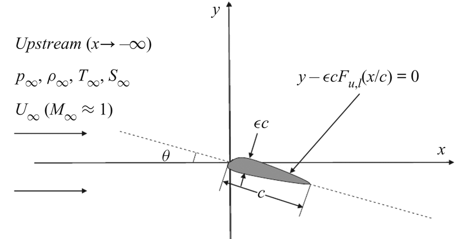
Figure 1. Flow problem.
Subindices  $x$ and
  $y$ denote partial derivatives with respect to axial and transverse coordinates, respectively. Here, the specific total enthalpy
  $h_T$ is expressed as,
  $\rho h_T = (\rho (u^2+v^2))/2 +\rho h $, where
  $h$ is the specific enthalpy of the gas. A general equation of state describes the thermodynamic behaviour of the gas
 \begin{equation} p = f(\rho,T). \end{equation}
 Using (2.3) and (2.6), it may be noticed that  $h_T$ is fixed along a constant streamfunction line
  $\psi$ of a fluid element, where
  $\psi _y= \rho u$, and
  $\psi _x = -\rho v$. This is also valid across any shock waves in the flow domain. Also,
  $h_T = h_{T\infty }$ for all streamlines in the flow, where
  $h_{T\infty } = ({{U_\infty }^2}) /{2}+ h_\infty$. Therefore, the energy equation (2.6) becomes
 \begin{equation} \tfrac{1}{2} (u^2+v^2) + h = \tfrac{1}{2} {U_\infty}^2 + h_{\infty}.\end{equation}
The set of flow equations (2.3)–(2.5), (2.7) and (2.8) together describe the complex interactions between the flow and the thermodynamics of a steady, two-dimensional, compressible and inviscid real gas. The flow is tangential at the airfoil surface, i.e.
 \begin{equation} u Fa_x+v Fa_y ={-}u\epsilon( F_{u,l})_{\bar{x}} + v=0 \quad {\rm on} \ \bar{y}= \epsilon F_{u,l}(\bar{x}),\quad 0\leqslant \bar{x} \leqslant 1 . \end{equation}
Also, the Kutta condition is satisfied at the sharp trailing edge of the airfoil, i.e. the pressures of the flow along the upper and lower surfaces of the airfoil are equal at the sharp trailing edge, i.e.  $p(c, y_{TE}^+) = p(c, y_{TE}^-)$. Also, since the upstream flow is uniform
 \begin{equation} u \rightarrow U_\infty, \quad v \rightarrow 0,\quad \rho \rightarrow \rho_\infty, \quad p \rightarrow p_\infty \quad {\rm as} \ x \rightarrow -\infty. \end{equation}
 The thin airfoil produces small perturbations to the uniform free-stream properties in all flow regions except the nose region, which is a small region  $O(\epsilon ^2)$ around the leading edge. In this region, the disturbances are of a higher order of magnitude due to rapid flow velocity changes. Therefore, the flow field of the gas may be described by an asymptotic TSD model in the entire flow domain around the airfoil outside the nose region. This model describes all the flow properties by asymptotic expansions of small perturbations to uniform free-stream properties caused by the thin airfoil. The derivation of this model is presented in the next section.
3. TSD theoretical model
Following the approach of Cole & Cook (Reference Cole and Cook1986) and Rusak & Lee (Reference Rusak and Lee2000a), the flow properties of the real gas may be approximated by asymptotic expansions
 \begin{equation} \left. \begin{gathered} \displaystyle \bar{p} = \frac {p}{p_\infty} = 1+ \epsilon^{2/3}\bar{p}_1 +\epsilon^{4/3}\bar{p}_2 + \cdots ,\\ \displaystyle \bar{T} = \frac {T}{T_\infty} = 1+ \epsilon^{2/3}\bar{T}_1 +\epsilon^{4/3}\bar{T}_2 + \cdots,\\ \displaystyle\bar\rho = \frac {\rho}{\rho_\infty} = 1+ \epsilon^{2/3}\bar\rho_1 +\epsilon^{4/3}\bar\rho_2 + \cdots, \\ \displaystyle\bar{u} =\frac {u}{U_\infty} = 1+ \epsilon^{2/3}\bar{u}_1 +\epsilon^{4/3}\bar{u}_2 + \cdots, \\ \displaystyle\bar{v}= \frac {v}{U_\infty} = \epsilon\bar{v}_1 +\epsilon^{5/3}\bar{v}_2 + \cdots. \\ \end{gathered}\right\} \end{equation}
The functions with subscripts 1 and 2 are non-dimensional perturbation functions of the similarity parameters of the flow problem and of the non-dimensional coordinates  $\bar {x}$ and
  $\tilde {y}$ where
 \begin{equation} \bar{x} = x/c, \quad \tilde{y} = \epsilon^{1/3} \bar{y}.\end{equation}
It should be noted that the non-dimensional transverse coordinate ( $\bar {y}$) is compressed by a factor of
  $\epsilon ^{1/3}$ to reflect the relatively large distance over which the uniform transonic axial flow is affected in the transverse direction compared to the axial direction. Also, a transonic similarity parameter,
  $K$, relates the upstream flow Mach number
  $M_\infty$ to the thickness ratio (
 $\epsilon$) of the airfoil
 \begin{equation} K = \frac{1-M_\infty^2}{\epsilon^{2/3}}.\end{equation}
Substitution of (3.1)–(3.3) into (2.3)–(2.5), (2.7) and (2.8), and a detailed derivation as given in Appendix A, results in the following equation
 \begin{equation} (K -K_G M_\infty^2 \bar{u}_1)\bar{u}_{1\bar{x}}+\bar{v}_{1\tilde{y}} = 0, \end{equation}
where
 \begin{align} K_G &={-}\frac{4RZ_\infty}{\bar{\gamma} C_v} \left( \frac{\partial \bar{p}}{\partial \bar{T}}\right)^2_\infty - \frac{2RZ_\infty}{\bar{\gamma} C_v} \left( \frac{\partial \bar{p}}{\partial \bar{T}}\right)_\infty \left( \frac{\partial \bar{p}}{\partial \bar \rho}\right)_\infty \nonumber\\ &\quad +\frac{2RZ_\infty}{\bar{\gamma} C_v} \left( \frac{\partial \bar{p}}{\partial \bar{T}}\right)_\infty \Bigg[\frac{\bar{\gamma}}{2} +1 \Bigg] +\frac{4RZ_\infty}{\bar{\gamma} C_v}\left( \frac{\partial^2 \bar{p}}{\partial \bar \rho \partial \bar{T}}\right)_\infty \left(\frac{\partial \bar{p}}{\partial \bar{T}}\right)_\infty \nonumber\\ &\quad +\frac{1}{\bar{\gamma}} \left[ \left( \frac{\partial^2 \bar{p}}{\partial \bar \rho^2}\right)_\infty +3\left(\frac{RZ_\infty}{C_v}\right)^2 \left( \frac{\partial^2 \bar{p}}{\partial \bar{T}^2}\right)_\infty \left(\frac{\partial \bar{p}}{\partial \bar{T}}\right)^2_\infty \right] + 2. \end{align}
In (3.5),  $Z_\infty = p_\infty /(\rho _\infty R T_\infty )$ is the compressibility factor of flow at upstream state,
  $C_v$ is the specific heat of gas at constant volume,
  $R = {\mathcal {R}}/\mu$ is the specific gas constant, where
  $\mu$ is the molecular weight of the gas and
  ${\mathcal {R}}$ is the universal gas constant, and
  $K_G$ is the thermodynamic similarity parameter and depends on the equation of state used to describe the relationships between the thermodynamic properties of the gas. It is related to the fundamental derivative of gas dynamics in the upstream state,
  $\varGamma _\infty$ as
 \begin{equation} K_G=2\varGamma_\infty. \end{equation}
In (3.5),  $\bar {\gamma }$ represents the effective specific heat ratio which relates the free-stream isentropic speed of sound to the free-stream thermodynamic properties and is expressed as
 \begin{equation} \bar{\gamma} =a_\infty^2 \frac{\rho_\infty}{p_\infty} = \frac{RZ_\infty}{C_v}\left(\frac{\partial \bar{p}}{\partial \bar{T}}\right)^2_\infty + \left( \frac{\partial \bar{p}}{\partial \bar \rho}\right)_\infty. \end{equation}
Also
 \begin{equation} \bar{u}_{1 \tilde{y}} - \bar{v}_{1 \bar{x}} = 0. \end{equation}
The set of equations (3.4) and (3.8) constitutes an extended Kármán–Guderley system for TSD flow of a gas. Flow has no vorticity and is isentropic in the leading order  $O(\epsilon ^{2/3})$ of perturbations in the temperature, density, pressure and velocity. Therefore, it can be described by a velocity perturbation potential function,
  $\phi _1$ where
  $\bar {u}_1 = \phi _{1\bar {x}}$ and
  $\bar {v}_1 = \phi _ {1\tilde {y}}$. Then, (3.4) becomes
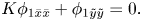
 \begin{equation} (K-K_G M_\infty^2 \phi_{1\bar{x}})\phi_{1 \bar{x}\bar{x}} + \phi_{1\tilde{y} \tilde{y}} =0. \end{equation}
Equation (3.9) is referred to as the modified TSD equation.
Substitution of the asymptotic equations (3.1) in the airfoil boundary conditions (2.9), the far-field conditions (2.10) and the Kutta condition gives
 \begin{equation} \left. \begin{gathered} \displaystyle \phi_{1\tilde{y} } (\bar{x}, 0^+) = F^{\prime}_{u}(\bar{x}) \quad {\rm and} \quad \phi_{1\tilde{y} } (\bar{x}, 0^-) = F^{\prime}_{l}(\bar{x}) \quad {\rm for} \ 0\leqslant \bar{x} \leqslant 1,\\ \displaystyle \phi_{1\bar{x} },\phi_{1\tilde{y} } \rightarrow 0\ {\rm as}\ \bar{x} \rightarrow -\infty, \quad \phi_{1\bar{x} } (1, 0^-) = \phi_{1\bar{x} } (1, 0^+). \end{gathered}\right\} \end{equation}
For the purposes of the numerical computations in the present study, the thermodynamic behaviour of the gas has been modelled according to the perfect-gas model, the van der Waals gas model, the cubic virial gas model and the Redlich–Kwong gas model. The thermodynamic similarity parameter  $K_G$ is derived for these gas models and relevant TSD equations are given in the following subsections.
3.1. TSD equation for the perfect-gas model
The perfect-gas equation of state to describe the thermodynamic behaviour of a gas is given as
 \begin{equation} p - R \rho T=0. \end{equation}
At low pressures and temperatures, the gas thermodynamic behaviour approaches the perfect-gas behaviour. Under these conditions,  $\bar {\gamma }= \gamma$,
  $({\partial \bar {p}}/{\partial \bar {T}})_\infty =1$ and
  $K_G = \gamma +1$ in (3.9) where
  $\gamma$ is the specific heat ratio of the gas. Equation (3.9) then becomes
 \begin{equation} [K-(\gamma+1) M_\infty^2 \phi_{1\bar{x}}]\phi_{1 \bar{x}\bar{x}} + \phi_{1\tilde{y} \tilde{y}} =0. \end{equation}
Equation (3.12) is the TSD equation for perfect-gas flow also given in Cole & Cook (Reference Cole and Cook1986).
3.2. TSD equation for the van der Waals gas model
The van der Waals equation of state (see Moran et al. Reference Moran, Shapiro, Boettner and Bailey2014) to describe the thermodynamic behaviour of a gas is given as
 \begin{equation} p = \frac{\rho R T}{1-\beta \rho} - \alpha \rho^2. \end{equation}
Coefficient  $\alpha$ represents the effects of the forces of attraction and repulsion between the molecules and the coefficient
  $\beta$ represents the effects of the finite size of the molecules. These effects become significant, especially for flow at high pressures and temperatures. The coefficients
  $\alpha$ and
  $\beta$ are related to the thermodynamic critical pressure (
 $p_c$) and critical temperature
  $(T_c)$ of the gas as
 \begin{equation} \alpha = \frac{27R^2T_c^2}{64 p_c}, \quad \beta = \frac{RT_c}{8p_c}. \end{equation}
 Using (3.7), the van der Waals gas specific heat ratio ( $\bar {\gamma }_{vdw}$) can be written as
 \begin{equation} \bar{\gamma}_{vdw} = \frac{RZ_\infty}{C_v}\left(1+ \frac{\alpha \rho^2_\infty}{p_\infty}\right)^2 + \frac{1}{1- \beta \rho_\infty}\left[1+ \frac{\alpha \rho^2_\infty}{p_\infty}\right] - \frac{2\alpha \rho^2_\infty}{p_\infty}. \end{equation}
The modified TSD equation for a van der Waals gas flow is
 \begin{equation} (K-K_{G\ vdw} M_\infty^2 \phi_{1\bar{x}})\phi_{1 \bar{x}\bar{x}} + \phi_{1\tilde{y} \tilde{y}} =0, \end{equation}
where
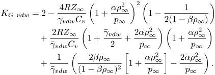 \begin{align} K_{G\ vdw} &= 2- \frac{4RZ_\infty}{\bar{\gamma}_{vdw} C_v}\left(1+ \frac{\alpha \rho^2_\infty}{p_\infty} \right)^2 \left(1-\frac{1}{2(1- \beta \rho_\infty)} \right) \nonumber\\ &\quad+\frac{2RZ_\infty}{\bar{\gamma}_{vdw} C_v} \left(1+\frac{\bar{\gamma}_{vdw}}{2}+ \frac{2\alpha \rho^2_\infty}{p_\infty} \right) \left(1+ \frac{\alpha \rho^2_\infty}{p_\infty} \right) \nonumber\\ &\quad+\frac{1}{\bar{\gamma}_{vdw}} \left( \frac{2\beta \rho_\infty}{(1- \beta \rho_\infty)^2}\left[1+ \frac{\alpha \rho^2_\infty}{p_\infty}\right] - \frac{2\alpha \rho^2_\infty}{p_\infty}\right). \end{align}
3.3. TSD equation for the cubic virial gas model
The cubic virial equation of state can be expressed as follows (see Moran et al. Reference Moran, Shapiro, Boettner and Bailey2014)
 \begin{equation} p = \rho R T + B\rho^2R T + C\rho^3R T. \end{equation}
In (3.18), the second virial coefficient  $B$ represents bimolecular attraction forces, and the third virial coefficient
  $C$ represents the repulsive forces among three molecules in close contact. At the critical state, the coefficients
  $B$ and
  $C$ can be solved in close form. Imposing the critical conditions
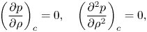 \begin{equation} \left(\frac{\partial p}{\partial \rho}\right)_c =0, \quad \left(\frac{\partial^2p}{\partial \rho^2}\right)_c =0, \end{equation}
the cubic virial equation can be solved to yield
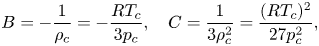 \begin{equation} B ={-}\frac{1}{\rho_c} ={-}\frac{R T_c}{3p_c}, \quad C = \frac{1}{3\rho_c^2} = \frac{(R T_c)^2}{27 p^2_c}, \end{equation}
where  $\rho _c$ is the critical density of the gas at critical temperature
  $T_c$ and critical pressure
  $p_c$. The compressibility factor
  $Z_c$ at the critical state is 0.333, compared to 0.375 for the van der Waals equation of state.
Using (3.7), the virial gas specific heat ratio ( $\bar {\gamma }_{virial}$) can be expressed as
 \begin{equation} \bar{\gamma}_{virial} = \frac{R}{C_vZ_\infty} \left[ 1+B \rho_\infty + C \rho_\infty^2 \right]^2 + \frac{1}{Z_\infty} \left[ 1+ 2B \rho_\infty + 3C \rho_\infty^2\right]. \end{equation}
The modified TSD equation for a virial gas flow is
 \begin{equation} (K-K_{G\ virial} M_\infty^2 \phi_{1\bar{x}})\phi_{1 \bar{x}\bar{x}} + \phi_{1\tilde{y} \tilde{y}} =0, \end{equation}
where
 \begin{align} K_{G\ virial} &= 2- \frac{4R}{\bar{\gamma}_{virial} C_vZ_\infty }\left( 1+B \rho_\infty + C \rho_\infty^2 \right)^2 + \frac{2R}{\bar{\gamma}_{virial} C_v} \left( 1+B \rho_\infty + C \rho_\infty^2 \right)\nonumber\\ &\quad \times \left[\left( 1+ \frac{\bar{\gamma}_{virial}}{2} \right)+\frac{1}{Z_\infty}\left( 1+2B \rho_\infty + 3C \rho_\infty^2 \right)\right]\notag\\ &\quad + \frac{1}{Z_\infty \bar{\gamma}_{virial}}\left( 2B\rho_\infty + 6C \rho_\infty^2 \right). \end{align}
3.4. TSD equation for the Redlich–Kwong gas model
The Redlich–Kwong equation of state is given as (see Moran et al. Reference Moran, Shapiro, Boettner and Bailey2014)
 \begin{equation} p = \frac{\rho R T}{1-b\rho} - \frac{a\rho^2}{\sqrt{T}(1+b\rho)}, \end{equation}
where  $a$ is a constant that corrects for intermolecular forces, and
  $b$ is a constant that corrects for the finite volume of the molecules. The constants can be calculated from the critical thermodynamic properties (
 $T_c, p_c$) of the gas
 \begin{equation} a = 0.42748 \frac{R^2T_c^{2.5}}{p_c}, \quad b = 0.08664 \frac{R T_c}{p_c}. \end{equation}
 Using (3.7), the Redlich–Kwong gas specific heat ratio ( $\bar {\gamma }_{rk}$) can be expressed as
 \begin{align} \bar{\gamma}_{rk} &= \frac{R Z_\infty}{C_{vv}} \left(\frac{1}{Z_\infty(1-b\rho_\infty)} + \frac{a\rho_\infty^2}{2\sqrt{T_\infty}p_\infty(1+b\rho_\infty)}\right)^2 + \frac{1}{Z_\infty(1-b\rho_\infty)^2} \nonumber\\ &\quad - \frac{a\rho_\infty^2 (2+b \rho_\infty)}{\sqrt{T_\infty}p_\infty(1+b\rho_\infty)^2}. \end{align}
The modified TSD equation for a Redlich–Kwong gas flow is
 \begin{equation} (K-K_{G rk} M_\infty^2 \phi_{1\bar{x}})\phi_{1 \bar{x}\bar{x}} + \phi_{1\tilde{y} \tilde{y}} =0, \end{equation}
where
 \begin{align} K_{G rk} &= 2- \frac{4RZ_\infty}{\bar{\gamma}_{rk} C_{vv} } \left( \frac{1}{Z_\infty(1-b\rho_\infty)} + \frac{a\rho_\infty^2}{2\sqrt{T_\infty}p_\infty(1+b\rho_\infty)} \right)^2 \nonumber\\ &\quad + \frac{2RZ_\infty}{\bar{\gamma}_{rk} C_{vv} } \left( \frac{1}{Z_\infty(1-b\rho_\infty)} + \frac{a\rho_\infty^2}{2\sqrt{T_\infty}p_\infty(1+b\rho_\infty)}\right) \left( \frac{1}{Z_\infty(1-b\rho_\infty)^2}\right.\nonumber\\ &\quad \left.+ \frac{2a\rho_\infty^2 (2+b \rho_\infty)}{\sqrt{T_\infty}p_\infty(1+b\rho_\infty)^2}\right) + \frac{2RZ_\infty}{\bar{\gamma}_{rk} C_{vv} } \left( \frac{\bar{\gamma}_{rk}}{2} +1\right)\nonumber\\ &\quad \times \left( \frac{1}{Z_\infty(1-b\rho_\infty)} + \frac{a\rho_\infty^2}{2\sqrt{T_\infty}p_\infty(1+b\rho_\infty)}\right)\nonumber\\ &\quad + \frac{1}{\bar{\gamma}_{rk}} \left[ \left( \frac{2b \rho_\infty}{Z_\infty(1-b\rho_\infty)^3} - \frac{2a\rho_\infty^2}{\sqrt{T_\infty}p_\infty(1+b\rho_\infty)} + \frac{2ab\rho_\infty^3 (2+b \rho_\infty)}{\sqrt{T_\infty}p_\infty(1+b\rho_\infty)^3} \right)\right. \nonumber\\ &\quad - 3 \left(\frac{RZ_\infty}{\bar{\gamma}_{rk} C_{vv} }\right)^2 \left( \frac{3a\rho_\infty^2}{4\sqrt{T_\infty}p_\infty(1+b\rho_\infty)} \right) \nonumber\\ &\quad \times\left.\left(\frac{1}{Z_\infty(1-b\rho_\infty)} + \frac{a\rho_\infty^2}{2\sqrt{T_\infty}p_\infty(1+b\rho_\infty)}\right)^2 \right]. \end{align}
3.5. Summary of the asymptotic model
The asymptotic analysis gives a nonlinear and homogeneous partial differential equation (3.9) to describe the field of the velocity perturbation potential ( $\phi _1$). The far-field and airfoil boundary conditions are given by (3.10). The numerical solution of (3.9) requires an iterative process to compute the field of
  $\phi _1 (\bar {x}, \tilde {y})$, which then provides the pressure field,
  $\bar {p} = p/p_\infty = 1- \epsilon ^ {{2}/{3}}( a_\infty ^2 M_\infty ^2\rho _\infty /p_\infty ) \phi _{1 \bar {x}}+\cdots$, the density field
  $\bar \rho = \rho /\rho _\infty = 1- \epsilon ^ {{2}/{3}}M_\infty ^2\phi _{1 \bar {x}}+\cdots$, the axial velocity field
  $u/ U_\infty = 1+ \epsilon ^{{2}/{3}} \phi _{1 \bar {x}}+\cdots$, the transverse velocity field
  $v/U_\infty = \epsilon \phi _{1 \bar {y}}+\cdots$ and the temperature field
  $T/T_\infty = 1 - \epsilon ^ {{2}/{3}} M_\infty ^2 (RZ_\infty )/(C_v) (\partial \bar {p}/\partial \bar {T})_\infty \phi _{1 \bar {x}}+\cdots$. The pressure coefficient (
 $C_p$) is computed as
  $C_p = (p-p_\infty )/((\rho _\infty U_\infty ^2)/{2}) = -2\epsilon ^ {{2}/{3}}\phi _{1\bar {x}}+ \cdots$. The wave drag coefficient of the flow around the airfoil,
  $C_d$, can be obtained by integrating the pressure distribution along the airfoil surface
 \begin{equation} C_d =\epsilon \int_{0}^{1} [(C_p)_{u}F^{\prime}_{u}-(C_p)_{l} F^{\prime}_{l}] \,\textrm{d}\bar{x}, \end{equation}
where  $u,l$ represent the upper and lower airfoil surfaces.
The model also identifies the similarity parameters that govern the flow physics which are: the thickness ratio of the airfoil  $\epsilon$, the scaled angle of attack
  $\varTheta$, the classical transonic similarity parameter
  $K$ and the thermodynamic similarity parameter
  $K_G$. The theory applies to any working fluid of interest.
The TSD equation (3.9) solution is characterized by a nose singularity (Cole & Cook Reference Cole and Cook1986; Rusak Reference Rusak1993) at the flow stagnation point near the airfoil's leading edge ( $\bar {x}\rightarrow 0, \tilde {y}\rightarrow 0$). The singularity affects the TSD solution in a small region
  $O(\epsilon ^2)$ around the airfoil's nose. The nose singularity causes the flow to be nearly symmetric around the leading edge as the upstream flow Mach number approaches unity, resulting in a loss of leading edge suction and lift, with respect to subsonic flows. In regions away from the leading edge of the order of
  $\epsilon$ and lower, the TSD model solution is not affected by the nose singularity. In the current study, the nose singularity is removed from the solutions following the approach of Rusak (Reference Rusak1993) and replacing
  $\gamma +1$ with
  $K_G$ in his analysis. After removal of the nose singularity, the TSD solution shows better agreement with an Euler flow solution around the leading edge.
4. Numerical algorithm
The TSD equation (3.9) is a nonlinear and homogeneous partial differential equation whose type depends on the value of  $[K - K_G M_\infty ^2 \phi _{1\bar {x}}]$. If
  $[K - K_G M_\infty ^2 \phi _{1\bar {x}}]>0$, then the equation is elliptic, if
  $[K - K_G M_\infty ^2 \phi _{1\bar {x}}]<0$, then the equation is hyperbolic and if
 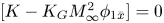 $[K - K_G M_\infty ^2 \phi _{1\bar {x}}]=0$, the equation is parabolic.
The seminal paper of Murman & Cole (Reference Murman and Cole1971) developed a numerical method to solve the type-changing partial differential equation encountered in the TSD study of steady and inviscid flow of dry air around airfoils. Separate finite-difference formulae were applied to discretize the equation in the elliptic (subsonic) and hyperbolic (supersonic) regions of transonic flow. The finite-difference equations were then solved iteratively in the computational domain using a line relaxation algorithm. The flow solution method naturally captures supersonic regions and shock waves around the airfoil. Cole & Cook (Reference Cole and Cook1986) included a numerical test to identify an approximated shock wave location. A mixed finite-difference scheme was then applied that used elements of forward and backward difference schemes to discretize the small-disturbance equation at the approximated shock wave location. Then, the predicted shock wave strength and location were found to match with experimental data. In the current study, a numerical algorithm based on the works of Cole & Cook (Reference Cole and Cook1986) and Krupp & Murman (Reference Krupp and Murman1972) is used. Details of the approach can also be found in Virk & Rusak (Reference Virk and Rusak2019, Reference Virk and Rusak2020), where similar flow problems are studied.
The TSD model effectively describes the flow in all regions except the nose region (of the order of  $\epsilon ^2$). It is well known that small-disturbance models produce a singularity in their computed solution around the leading edge (Cole & Cook Reference Cole and Cook1986). In the current study, the method of Rusak (Reference Rusak1993) is used to remove the nose singularity and form a composite solution which describes flow in the nose region as well as regions away from the nose. Details of the approach can be found in Rusak (Reference Rusak1993). The current numerical algorithm is second-order accurate in space; except across shock wave points, where it is first-order accurate. The converged solution is used to plot the distributions of the pressure coefficient along the surface of the thin airfoil. Integration of the pressure distribution on the airfoil surfaces is used to compute the wave drag coefficient. The solution is also used to plot the pressure–temperature phase diagram of flow along a streamline close to the airfoil.
5. Computed results
In this section, non-lifting flow problems in the subsonic and transonic regimes of single-phase subcritical, near-critical and supercritical fluids are studied using the TSD models for various equations of state derived in § 3. The TSD numerical results based on the different models are compared, to explore the effects of thermodynamic modelling on flow solutions in the different flow regimes. Furthermore, the sensitivity of the flow behaviour to changes in free-stream thermodynamic conditions are studied. The theory is used to explore the relationship between the upstream flow thermodynamic state of the gas and the critical upstream Mach number ( $M_c$) for the onset of shock waves in the case of flows around a NACA0012 airfoil (
 $\epsilon =0.12$) at zero angle of attack. We focus on water as an example of the working fluid.
5.1. Subsonic flows
For subsonic flows around thin airfoils ( $\epsilon \leqslant 0.12$) with low free-stream Mach number, typically with
  $M_\infty < 0.7$, as well as for supersonic flows, typically with
  $M_\infty >1.4$, the absolute value of the transonic similarity parameter
  $K$, becomes much greater in magnitude than the nonlinear term,
  $K_G M_\infty ^2 \phi _{1\bar {x}}$. Therefore, in such flow cases, the effects of the thermodynamic behaviour of the gas in the TSD equation (3.9) may be neglected and it may be reduced to
 \begin{equation} K\phi_{1 \bar{x}\bar{x}} + \phi_{1\tilde{y} \tilde{y}} =0. \end{equation}
Using the definition of  $\tilde {y} = \epsilon ^{1/3} \bar {y}$, it can be shown that (5.1) is equivalent to the classical Prandtl–Glauert equation (Kuethe & Chow Reference Kuethe and Chow1976) for linearized subsonic and supersonic flow behaviours around thin airfoils
 \begin{equation} (1-M_\infty^2)\phi_{1 \bar{x}\bar{x}} + \phi_{1\bar{y} \bar{y}} =0. \end{equation}
Equation (5.2) suggests that the physical behaviour of subsonic or supersonic flows around thin airfoils is nearly independent of the equation of state used to describe the gas thermodynamic behaviour and of the upstream thermodynamic properties of the gas (as long as  $M_\infty$ and the airfoil shape are fixed). Moreover, in these cases, flows are dominated by the classical solutions, no matter whether the upstream flow thermodynamic conditions are subcritical, near-critical or supercritical and are independent of value of
  $K_G$.
An example of a flow problem is solved to demonstrate this behaviour. Steam flow with free-stream conditions defined by  $M_\infty =0.6$,
  $T_\infty =575$ K and
  $p_\infty = 5.73$ MPa around a NACA0012 airfoil (
 $\epsilon =0.12$) at zero angle of attack (
 $\varTheta =0$) is studied. In this case, the flow all around the airfoil is subsonic and single phase with no condensation. Note that the upstream pressure and temperature are much higher than atmospheric properties. The problem is solved according to the perfect gas, van der Waals gas, cubic virial gas and Redlich–Kwong gas TSD models derived in § 3. For all cases,
  $K=2.63$ and
  $R/C_v =0.190$. The thermodynamic similarity parameter
  $K_G$ and upstream compressibility factor
  $Z_\infty$ are considerably smaller for the real-gas models compared to the perfect-gas model, due to high upstream pressure (as noted in table 1). The computations of this flow problem show that the term
  $K_G M_\infty ^2 \phi _{1\bar {x}}$ in (3.9) is insignificant compared to
  $K$ due to the low value of
  $M_\infty$ and small axial velocity perturbations (
 $\phi _{1\bar {x}}$). The distributions of the pressure coefficient (
 $-C_p$) along the airfoil surface from using the various TSD models are nearly the same and are described by the solution of the Prandtl–Glauert equation (5.2). The wave drag coefficient (
 $C_d$) is zero for all model solutions. A similar behaviour is found for all other single-phase subsonic flows and upstream thermodynamic conditions. Subsonic flow behaviour is independent of the thermodynamic modelling of the gas and of the upstream thermodynamic conditions of the gas.
Table 1. Values of  $K_G$,
  $Z_\infty$,
  $\bar {\gamma }$ and upstream fluid stagnation properties for the various equation of state TSD models at
  $M_\infty =0.6$,
  $T_\infty =575$ K and
  $p_\infty = 5.73$ MPa.
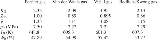
5.2. Transonic flows at low subcritical thermodynamic conditions
Steam flow with free-stream conditions defined by  $M_\infty =0.8$,
  $T_\infty =375$ K and
  $p_\infty = 0.011$ MPa around a NACA0012 airfoil (
 $\epsilon =0.12$) at zero angle of attack (
 $\varTheta =0$) is studied with the various gas TSD models. For all cases,
  $K=1.48$ and
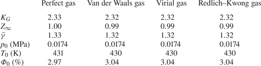
 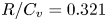 $R/C_v =0.321$. Values of
  $K_G$,
  $Z_\infty$,
  $\bar {\gamma }$ and the upstream stagnation conditions of fluid are given in table 2. Values of
  $K_G$,
  $\bar {\gamma }$ and
  $Z_\infty$ (approximately 1) are nearly the same for the different gas models. Figure 2 shows the distributions of the pressure coefficient (
 $-C_p$) along the airfoil surface from using the various TSD models. Figure 3 shows the pressure versus temperature phase diagram along a streamline close to the airfoil from the various TSD model solutions. Also shown for reference is the saturated vapour pressure versus temperature line. At subcritical flow conditions, the distributions of the pressure coefficient and the pressure versus temperature phase diagrams of the four gas models are nearly the same since the thermodynamic similarity parameter for the models is almost same (approximately 2.3). In the transonic flow regime,
  $K_G$ has a substantial effect on the flow field because the nonlinear term
  $K_G M_\infty ^2 \phi _{1\bar {x}}$ in (3.9) is considerably greater with respect to
  $K$ than in the subsonic case studied in § 5.1. Significant flow acceleration to supersonic speeds terminated by a strong shock wave (at
  $\bar {x} \sim 0.48$) is observed on the airfoil surface for all model solutions. Compared to the previous subsonic flow case, where the wave drag coefficient (
 $C_d$) was zero, in this case
  $C_d$ is found to be approximately 0.01 for all model solutions. A similar behaviour is observed for all other single-phase transonic flows at low subcritical thermodynamic upstream conditions. Transonic flow behaviour is independent of the thermodynamic modelling of the gas at such conditions.
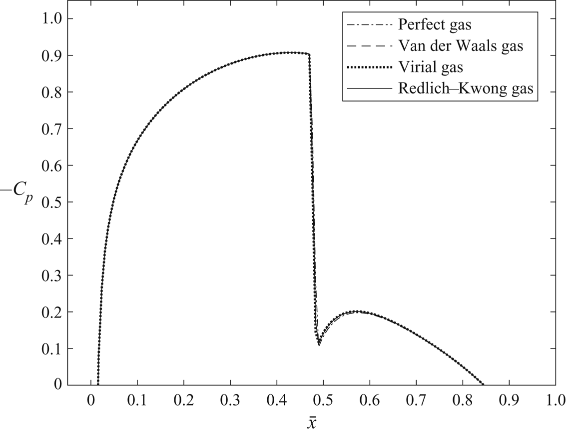
Figure 2. Distribution of the pressure coefficient ( $-C_p$) at NACA0012 airfoil (
 $\epsilon =0.12$) surface for steam flow at
  $M_\infty =0.8$,
  $T_\infty =375$ K,
  $p_\infty = 0.011$ MPa and
  $\varTheta = 0$ using various equation of state TSD models.
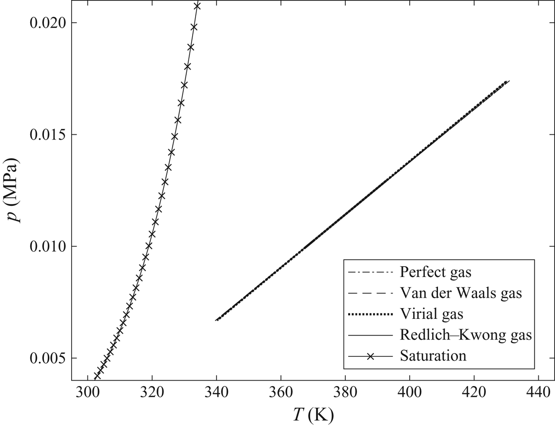
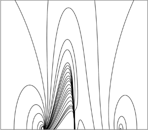
Figure 3. The  $p-T$ phase diagram along a streamline close to NACA0012 airfoil surface for steam flow at
  $M_\infty =0.8$,
  $T_\infty =375$ K,
  $p_\infty = 0.011$ MPa and
  $\varTheta = 0$ using various equation of state TSD models.
Table 2. Values of  $K_G$,
  $Z_\infty$,
  $\bar {\gamma }$ and upstream fluid stagnation properties for the various equation of state TSD models at
  $T_\infty =375$ K,
  $p_\infty = 0.011$ MPa and
  $M_\infty =0.8$.
5.3. Transonic flows at near-critical thermodynamic conditions
A steam flow problem with free-stream conditions defined by  $M_\infty =0.8$,
  $T_\infty =575$ K and
  $p_\infty = 5.73$ MPa around a NACA0012 airfoil (
 $\epsilon =0.12$) at zero angle of attack (
 $\varTheta =0$) is studied with the different gas TSD models. In this case, upstream flow thermodynamic conditions are near critical. For all models,
  $K=1.48$ and
  $R/C_v =0.190$ (same as in § 5.1). Values of
  $K_G$,
  $Z_\infty$,
  $\bar {\gamma }$ and the upstream fluid stagnation properties for the various models are given in table 3. Note that, whenever the stagnation temperature is greater than the critical temperature of the fluid, the relative humidity value is not reported. This refers to the fact that a vapour saturation pressure does not exist at temperatures above the critical temperature. The distributions of the pressure coefficient (
 $-C_p$) for the different TSD models are shown in figure 4. Figure 5 shows the pressure–temperature phase diagram along a streamline close to the airfoil surface for the models. Also shown for reference in figure 5 is the saturated vapour pressure line. It can be seen that the flow remains superheated in all regions around the airfoil.
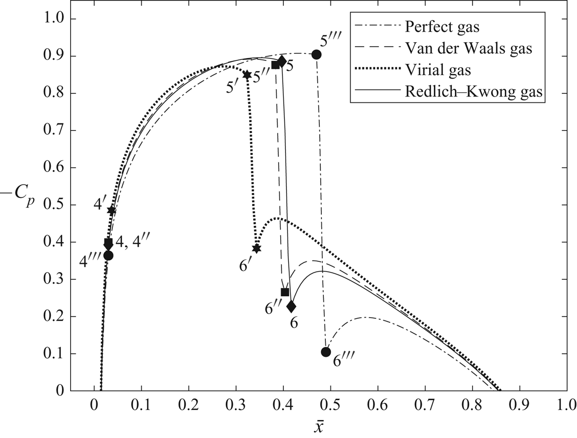
Figure 4. Distribution of the pressure coefficient ( $-C_p$) at NACA0012 airfoil surface for steam flow at
  $M_\infty =0.8$,
  $T_\infty =575$ K,
  $p_\infty = 5.73$ MPa and
  $\varTheta = 0$ using various equation of state TSD models.
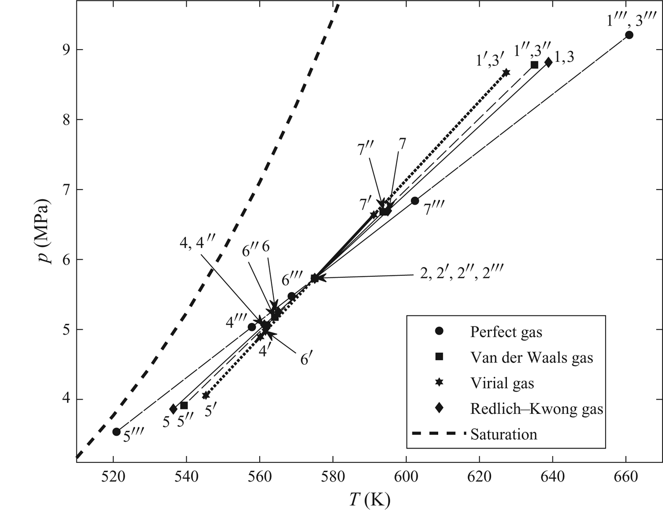
Figure 5. The  $p-T$ phase diagram along a streamline close to NACA0012 airfoil surface for steam flow at
  $M_\infty =0.8$,
  $T_\infty =575$ K,
  $p_\infty = 5.73$ MPa and
  $\varTheta = 0$ using various equation of state TSD models.
Table 3. Values of  $K_G$,
  $Z_\infty$,
  $\bar {\gamma }$ and upstream fluid stagnation properties for the various equation of state TSD models at
  $M_\infty =0.8$,
  $T_\infty =575$ K and
  $p_\infty = 5.73$ MPa.
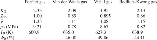
Figures 4 and 5 also show important characteristic points in the flow which help to better understand the flow dynamics. Point 1 is the stagnation state of the upstream fluid and point 2 is the upstream state of flow. As the flow approaches the airfoil, it decelerates, gets compressed and reaches stagnation point 3 at the nose of the airfoil. After that, the flow accelerates along the airfoil surface. Velocity increases and pressure and temperature decrease, until the flow becomes sonic (point 4). The flow keeps accelerating beyond the sonic point and becomes supersonic, and expands to minimum values of local pressure and temperature (point 5). A compression shock wave occurs and the pressure and temperature behind it increase to point 6. For a small region downstream of the shock wave, the flow exhibits classical Zierep shock wave behaviour (Oswatitsch & Zierep Reference Oswatitsch and Zierep1960), where the pressure and temperature decrease and then increase with distance from the shock wave. As the flow approaches the trailing edge of the airfoil (point 7), its velocity decreases and pressure and temperature increase. Behind the trailing edge, the flow accelerates and pressure and temperature decrease to upstream flow conditions.
In the nose region of the airfoil, the pressure fields for all gas models are nearly the same but, upon moving downstream along the airfoil surface, the difference between the computed solutions increases. Perfect-gas model (marked by circles in figure 4) captures the strongest shock wave and it is located farthest downstream from the leading edge along the airfoil surface (at  $\bar {x} \sim 0.48$) relative to the other models. The shock waves computed by the Redlich–Kwong gas model (marked by diamonds in figure 4) and the van der Waals gas model (marked by squares in figure 4) are weaker than in the perfect-gas case and are located relatively upstream at
  $\bar {x} \sim 0.40$ and at
  $\bar {x} \sim 0.38$, respectively. The shock wave computed by the virial gas model (marked by stars in figure 4) is even weaker in strength and located upstream relative to the other models (at
  $\bar {x} \sim 0.32$). At high near-critical temperatures and pressures, such as this flow problem, the Redlich–Kwong gas model is expected to approximate the flow fields most accurately. Hence, under these conditions, the perfect-gas model tends to over-estimate the shock wave strength and consequently the pressure drag of the airfoil, given in table 4. Figure 6 shows contours of
  $C_p$ around the airfoil surface from the Redlich–Kwong gas TSD solution. The shock wave can be observed as a nearly vertical black line which is curved upstream and is formed due to coalescence of
  $C_p$ contours on the airfoil surface at
  $\bar {x} \sim 0.40$.
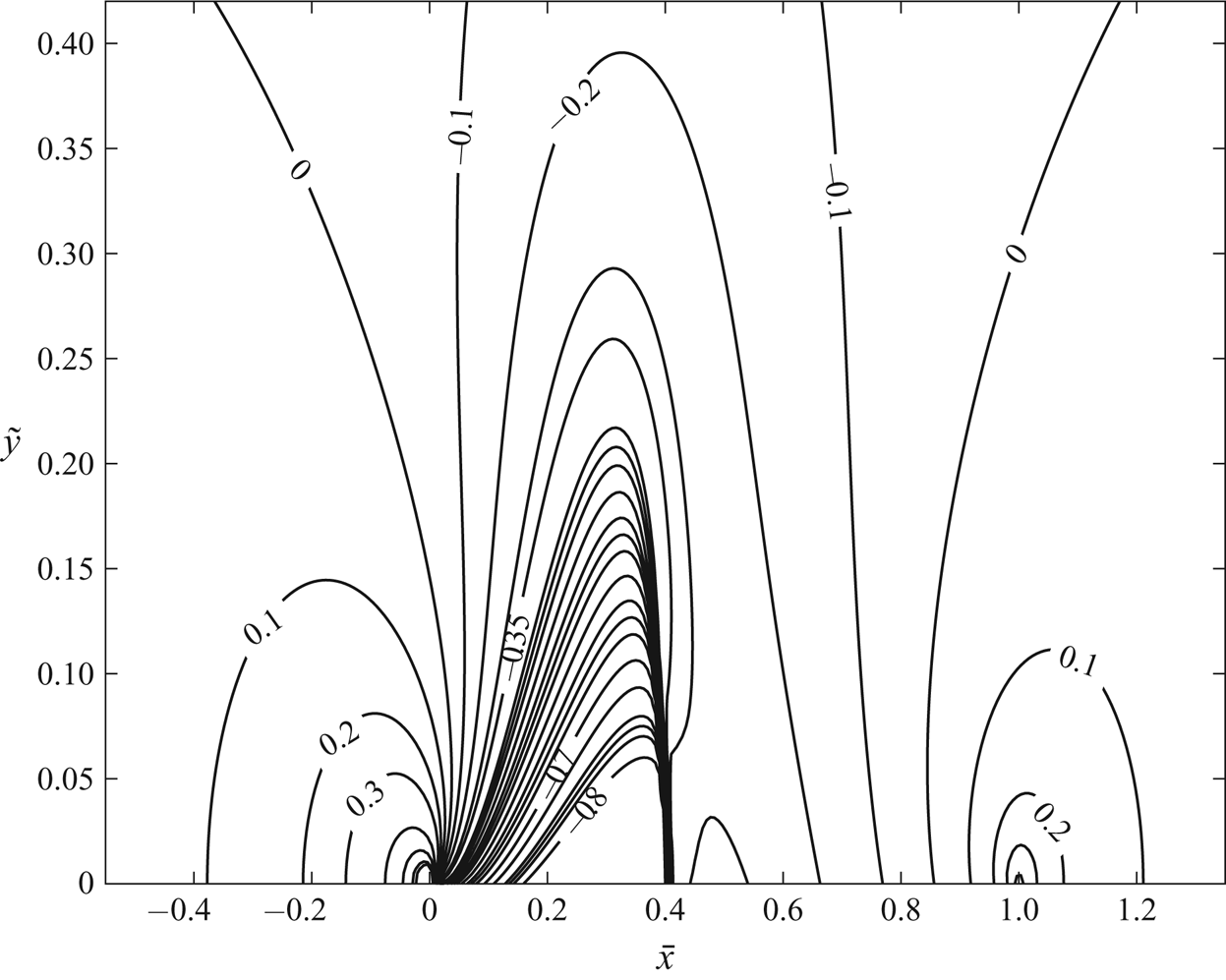
Figure 6. Contours of  $C_p$ for steam flow around a NACA0012 airfoil (
 $\epsilon =0.12$) at
  $M_\infty =0.8$,
  $T_\infty =575$ K,
  $p_\infty = 5.73$ MPa and
  $\varTheta = 0$, according to the Redlich–Kwong gas TSD model.
Table 4. Pressure drag coefficient  $C_d$ for the various equation of state TSD model solutions at the described conditions.
In the transonic flow regime, as the thermodynamic similarity parameter  $K_G$ decreases, the shock wave becomes weaker and moves upstream along the airfoil surface, consequently reducing the wave drag of the airfoil. Note that
  $K_G$ depends only on the upstream conditions of
  $p_\infty$ and
  $T_\infty$. At fixed upstream conditions of pure steam described by
  $T_\infty = 575$ K, the variations in
  $K_G$ for the different models with
  $p_\infty$ are shown in figure 7. While the
  $K_G$ for perfect gas stays fixed at 2.33,
  $K_G$ for the other gas models decreases monotonically with an increase in
  $p_\infty$. In addition, figure 8 shows the variation in
  $K_G$ for the different models with increasing values of
  $T_\infty$ at a fixed value of
  $p_\infty =5.73$ MPa. The
  $K_G$ for the perfect-gas model stays fixed at 2.33, while
  $K_G$ for the other gas models decreases monotonically and nonlinearly with an increase of
  $T_\infty$. It is interesting to note that
  $K_G$ values for all models are nearly the same for
  $T_\infty < 400$ K at the given
  $p_\infty =5.73$ MPa. Therefore, the perfect-gas equation of state adequately describes the thermodynamics of steam flow under such conditions.
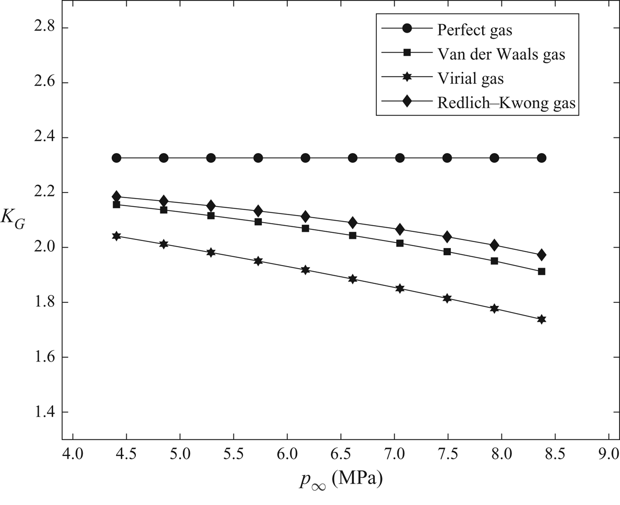
Figure 7. Thermodynamic similarity parameter  $K_G$ for steam flow at
  $T_\infty =575$ K for various values of
  $p_\infty$.
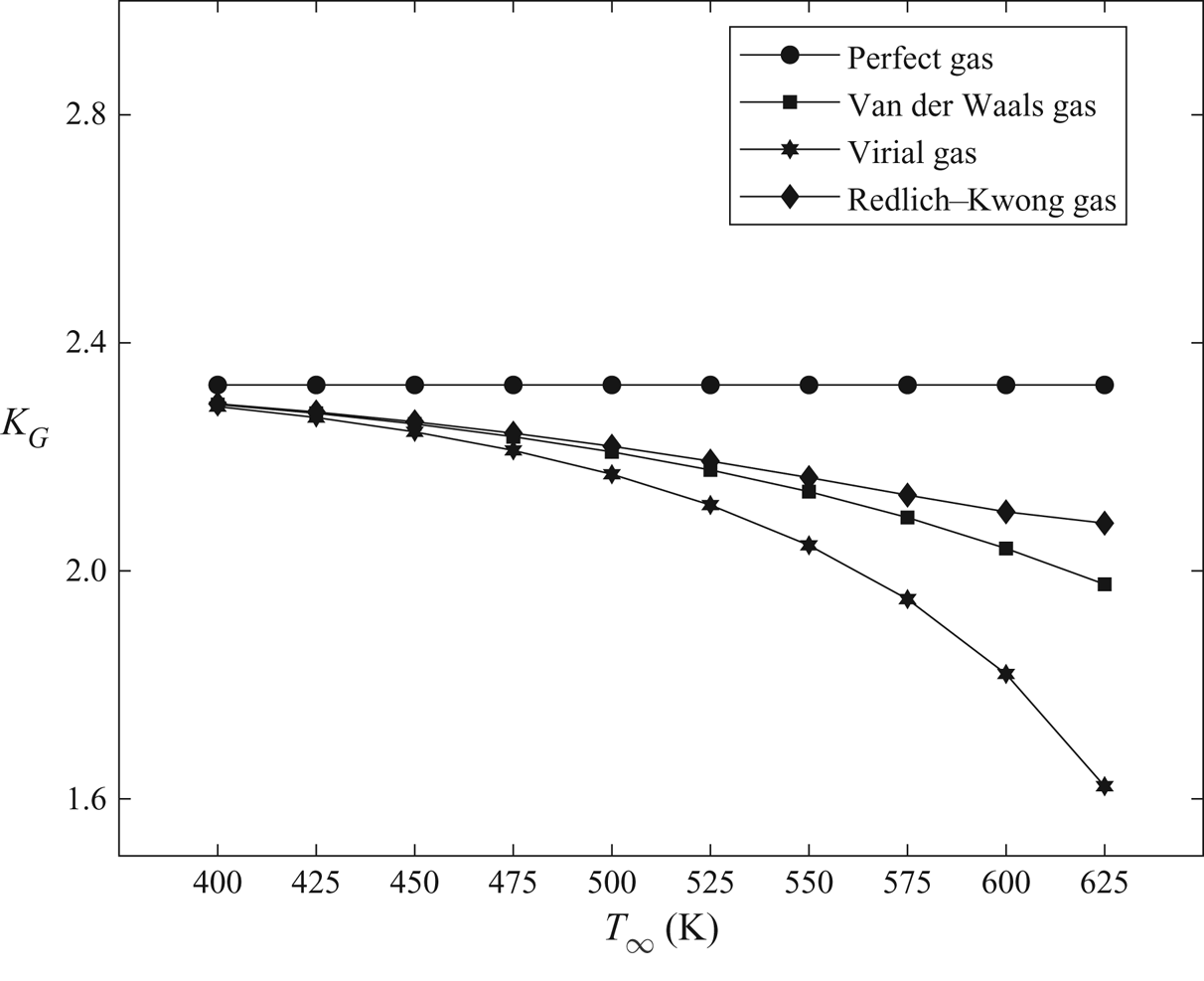
Figure 8. Thermodynamic similarity parameter  $K_G$ for steam flow at
  $p_\infty =5.73$ MPa for various values of
  $T_\infty$.
5.4. Transonic flows at supercritical thermodynamic conditions
A flow problem in the supercritical flow regime is also solved using the various gas TSD models. Steam flow with free-stream conditions defined by  $M_\infty =0.8$,
  $T_\infty =712$ K (
 $T_r=1.1$) and
  $p_\infty = 24.3$ MPa (
 $p_r=1.1$) around a NACA0012 airfoil (
 $\epsilon =0.12$) at zero angle of attack (
 $\varTheta =0$) where
  $T_{r \infty }=T_\infty /T_c$ and
  $p_{r \infty } = p_\infty /p_c$ are the reduced temperature and reduced pressure, respectively, is studied. For all gas models,
  $K=1.48$ and
 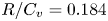 $R/C_v = 0.184$. Values of
  $K_G$,
  $Z_\infty$,
  $\bar {\gamma }$ and the upstream fluid stagnation properties for the respective models are given in table 5. The values of
  $K_G$,
  $Z_\infty$ and
  $\bar {\gamma }$ for the virial gas model are significantly lower than the corresponding values for the other gas models. For the van der Waals gas model,
  $K_G$,
  $Z_\infty$ and
  $\bar {\gamma }$ decrease below the values of the perfect-gas model. While, for the Redlich–Kwong gas model,
  $K_G$ becomes greater than the perfect-gas
  $K_G$. The compressibility factor
  $Z_\infty$ for the virial gas is also close to its critical compressibility factor (
 $Z_c = 0.33$).
Table 5. Values of  $Z_\infty$,
  $K_G$,
  $R/C_v$ and
  $\bar {\gamma }$ for the various equation of state TSD models solutions at
  $T_\infty =712$ K,
  $p_\infty = 24.3$ MPa and
  $M_\infty =0.8$.
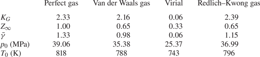
The distributions of the pressure coefficient ( $-C_p$) for various equation of state TSD models are shown in figure 9 along with the characteristic flow points as defined in § 5.3. In all cases, the flow is superheated in all regions around the airfoil. No shock wave is observed in the virial gas model solution, where the flow stays subsonic in all flow regions. On the other hand, the perfect gas, van der Waals gas and Redlich–Kwong gas TSD solutions exhibit shock waves on the airfoil surface. The strength of the shock wave increases as
  $K_G$ increases, and the shock wave shifts downstream on the airfoil surface. The Redlich–Kwong gas model produces the strongest shock wave (at
  $\bar {x} \sim 0.5$) which is located downstream compared to the perfect-gas model (at
  $\bar {x} \sim 0.48$) and the van der Waals gas model (at
  $\bar {x} \sim 0.39$). Figure 10 shows the pressure–temperature phase diagram along a streamline close to the airfoil surface for the models. Also shown for reference is the vapour–liquid saturation pressure line including the critical point. The
  $p-T$ diagrams of the Redlich–Kwong gas and van der Waals gas are close in terms of ranges of variations in local pressure and temperature. Both models provide sufficiently accurate modelling of real-gas effects in the thermodynamic range under consideration, with the Redlich–Kwong gas model being slightly more accurate.
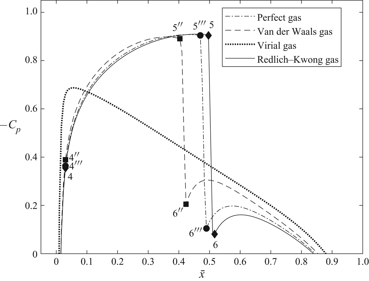
Figure 9. Distribution of the pressure coefficient ( $-C_p$) at NACA0012 airfoil (
 $\epsilon =0.12$) surface for steam flow at
  $T_\infty =712$ K,
  $p_\infty = 24.3$ MPa,
  $M_\infty =0.8$ and
  $\varTheta = 0$ using various equation of state TSD models.
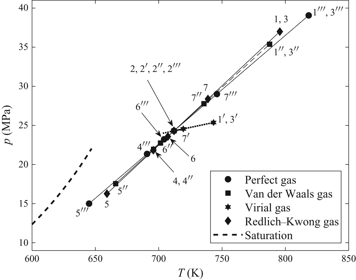
Figure 10. The  $p-T$ phase diagram along a streamline close to NACA0012 airfoil (
 $\epsilon =0.12$) surface for steam flow at
  $T_\infty =712$ K,
  $p_\infty = 24.3$ MPa,
  $M_\infty =0.8$ and
  $\varTheta = 0$ using various equation of state TSD models.
The pressure drag coefficients ( $C_d$) of the solutions of the various models are given in table 6. Virial gas model predicts zero wave drag because of the flow staying subsonic all around the airfoil and no occurrence of shock waves. Redlich–Kwong gas model predicts the highest wave drag followed by the perfect-gas model and van der Waals gas model according to the strength of the shock wave in their respective numerical solutions.
Table 6. Pressure drag coefficient  $C_d$ for the various equation of state TSD model solutions at the described conditions.
5.5. Transonic flows at high supercritical thermodynamic conditions
A flow problem in the high supercritical flow regime is also solved using the perfect gas, van der Waals gas and Redlich–Kwong gas TSD models. Virial gas model is not used in this case, since it predicts inaccurate values of the gas density at the given flow conditions. Steam flow with free-stream conditions defined by  $M_\infty =0.8$,
  $T_\infty =950$ K (
 $T_r=1.5$) and
  $p_\infty = 55$ MPa (
 $p_r=2.5$) around a NACA0012 airfoil (
 $\epsilon =0.12$) at zero angle of attack (
 $\varTheta =0$) is studied. For all gas models,
  $K=1.48$ and
  $R/C_v = 0.21$. Values of
  $K_G$,
  $Z_\infty$,
  $\bar {\gamma }$ and the upstream fluid stagnation properties for the respective models are given in table 7. Values of
  $Z_\infty$ and
  $\bar {\gamma }$ for the Redlich–Kwong gas model and van der Waals gas model are comparable. The values of
  $K_G$ for the Redlich–Kwong gas model and the van der Waals gas model are significantly greater than that for the perfect-gas model, as well as with respect to values in the previous cases.
Table 7. Values of  $Z_\infty$,
  $K_G$,
  $R/C_v$ and
  $\bar {\gamma }$ for the various equation of state TSD model solutions at
  $T_\infty =950$ K,
  $p_\infty = 55$ MPa and
  $M_\infty =0.8$.
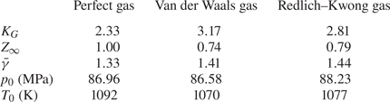
The distributions of the pressure coefficient ( $-C_p$) for the three TSD models are shown in figure 11 along with the characteristic flow points as defined in § 5.3. In all cases, flow is superheated in all regions around the airfoil. In this case, the perfect-gas model predicts the weakest shock wave (at
  $\bar {x} \sim 0.49$) which is located more upstream compared to the other models. Figure 12 shows the pressure–temperature phase diagram along a streamline close to the airfoil surface for the models. The pressure drag coefficients (
 $C_d$) of the solutions of the various models are given in table 8. The Redlich–Kwong gas model and van der Waals gas model predict higher wave drag followed by the perfect-gas model according to the strength of the shock wave in their respective numerical solutions.
Table 8. Pressure drag coefficient  $C_d$ for the various equation of state TSD model solutions at the described conditions.
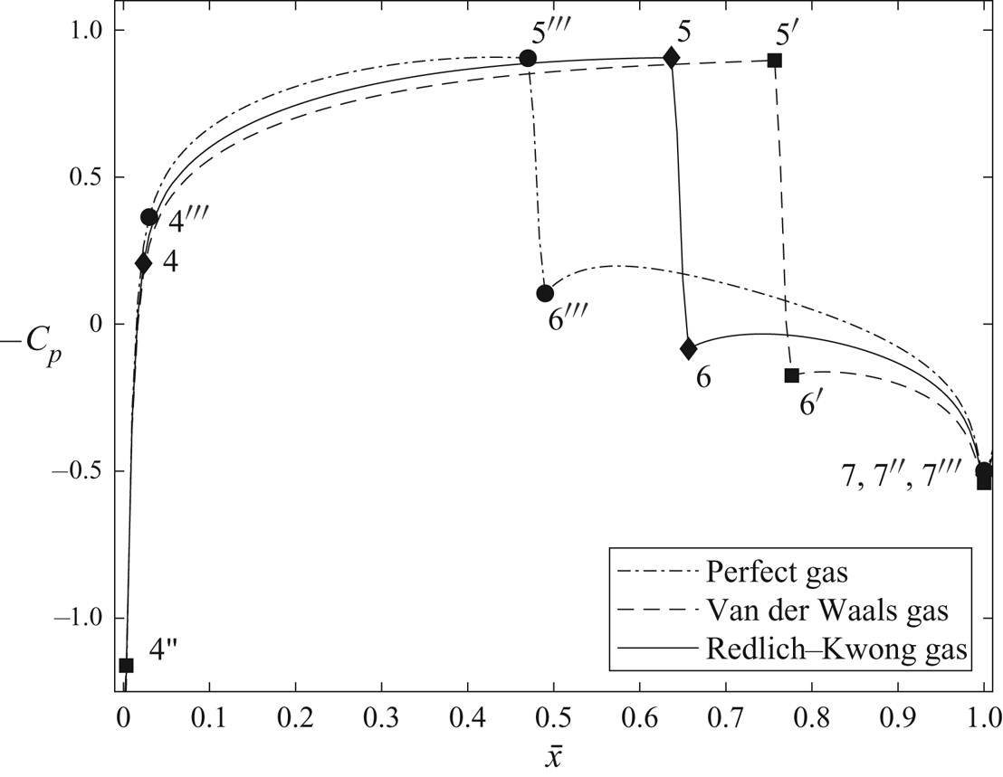
Figure 11. Distribution of the pressure coefficient ( $-C_p$) at NACA0012 airfoil (
 $\epsilon =0.12$) surface for steam flow at
  $T_\infty =950$ K,
  $p_\infty = 55$ MPa,
  $M_\infty =0.8$ and
  $\varTheta = 0$ using various equation of state TSD models.
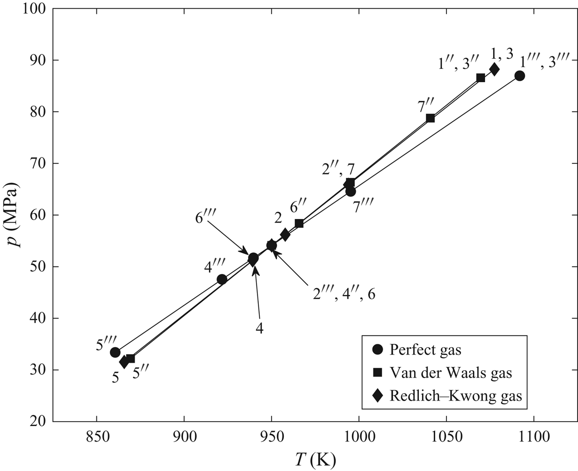
Figure 12. The  $p-T$ phase diagram along a streamline close to NACA0012 airfoil (
 $\epsilon =0.12$) surface for steam flow at
  $T_\infty =950$ K,
  $p_\infty = 55$ MPa,
  $M_\infty =0.8$ and
  $\varTheta = 0$ using various equation of state TSD models.
6. Discussion
6.1. Variation of  $K_G$ with upstream temperature and pressure

The computed results in §§ 5.1–5.5 demonstrate that the flow behaviour changes significantly with the increase of upstream temperature and pressure at a fixed Mach number and airfoil geometry, from low subcritical to high supercritical thermodynamic conditions. Specifically, the pressure and temperature distributions along the airfoil surface, the location and strength of the shock wave and the wave drag coefficient vary significantly. We attribute these changes to the significant nonlinear variations in  $K_G$ as a function of upstream pressure and temperature. To demonstrate this in more detail, the dependence of the thermodynamic similarity parameter
  $K_G$ on upstream thermodynamic conditions
  $T_\infty$ and
  $p_\infty$ is studied in different thermodynamic domains for water vapour thermodynamics modelled by the Redlich–Kwong gas model.
For water vapour flow at a fixed  $T_\infty$ below the critical temperature
  $T_c=647.3$ K and a pressure below the critical pressure
  $p_c=22.1$ MPa,
  $K_G$ was found to decrease continuously with an increase of the upstream pressure (
 $p_\infty$) until the saturation pressure, see figure 13. With an increase of
  $p_\infty$ at a fixed
  $T_\infty$, the influence of real-gas effects increases. This causes the compressibility factor
  $Z_\infty$ and the ratio
  $R/C_v$ of water vapour to decrease as well, and thereby, the term
  $(RZ_\infty )/(\bar {\gamma } C_v)$ in formula (3.5) for
  $K_G$ decreases. This primarily results in a decrease of
  $K_G$ in this range of temperatures and pressures below critical properties. The decrease of
  $K_G$,
  $Z_\infty$,
  $R/C_v$ and
  $(RZ_\infty )/(\bar {\gamma } C_v)$ with an increase of
  $p_\infty$ until the saturation pressure at a fixed
  $T_\infty = 600$ K can be seen in figure 14. As a result of the decrease in
  $K_G$ in the subcritical region, the nonlinear term in (3.9) becomes smaller compared to
  $K$, and thereby, transonic effects are delayed to higher Mach numbers and wave drag decreases in this operational region.
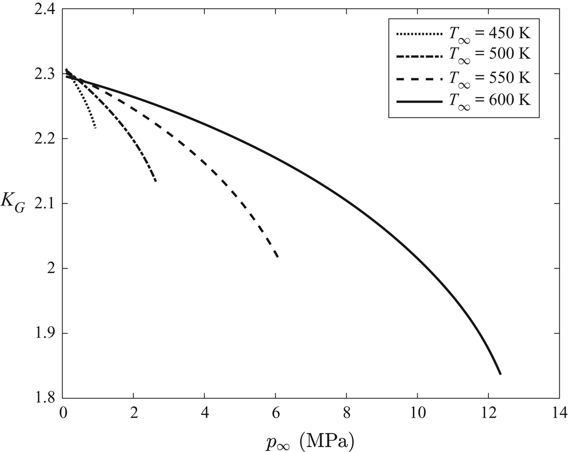
Figure 13. Thermodynamic similarity parameter  $K_G$ as a function of
  $p_\infty$ for several values of
  $T_\infty$ below the critical temperature.
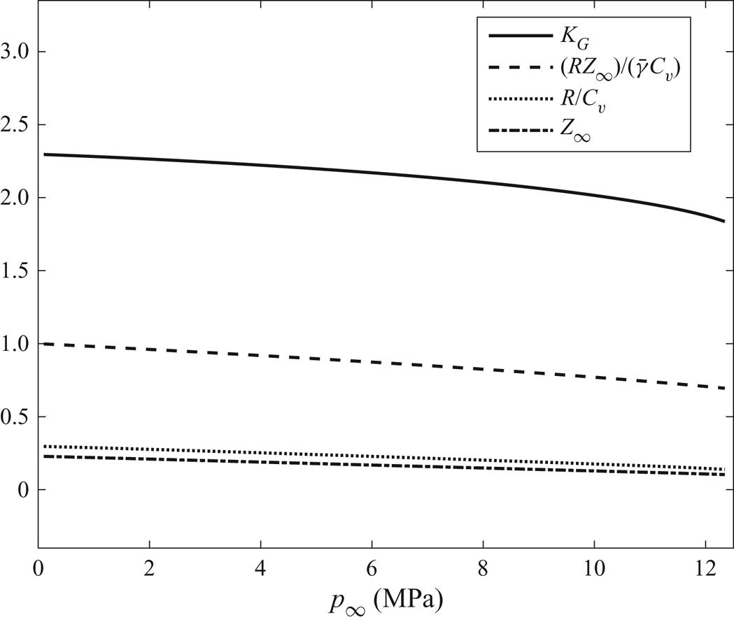
Figure 14. Change of  $K_G$,
  $(RZ_\infty )/(\bar {\gamma } C_v)$,
  $R/C_v$ and
  $Z_\infty$ with
  $p_\infty$ at a fixed
  $T_\infty =600$ K.
However, for water vapour flows with  $T_\infty > T_c$ and changing
  $p_\infty$ from atmospheric value (
 $p_\infty =0.1$ MPa) to much higher values (
 $p_\infty = 200$ MPa), we find that
  $K_G$ behaves differently, see figure 15. The values of
  $K_G$ decrease with pressure until water vapour reaches a pressure (
 $p_s$) where the flow entropy is equal to the critical gas entropy (
 $s=s_c=4.6\ \textrm {kJ}\ (\textrm {kgK})^{-1}$ for water vapour). An inflection point in the graph of
  $K_G$ versus
  $p_{\infty }$ appears at this
  $p_\infty =p_s$. Upon further increasing
  $p_\infty$,
  $K_G$ increases along nearly linear curves with the same slope of the curve irrespective of
  $T_{\infty }$. The decrease in
  $K_G$ for flow conditions with
  $s\leqslant s_c$ can be explained by figure 14. The different behaviour of real-gas effects at above critical temperatures and pressures is shown in figure 16. Specifically, the compressibility factor
  $Z_\infty$ increases with
  $p_\infty$ and, according to formula (3.5), it causes a significant increase of
  $K_G$ at supercritical thermodynamic conditions. As a result of an increase in
  $K_G$ in the supercritical region, the nonlinear term in (3.9) becomes larger compared to
  $K$, and thereby, transonic effects are advanced to lower Mach numbers and wave drag increases in this operational region.
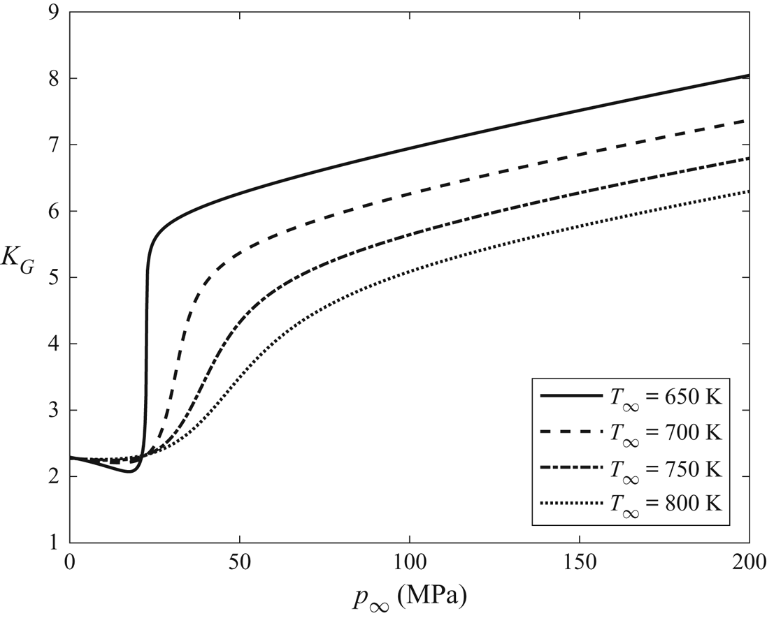
Figure 15. Thermodynamic similarity parameter  $K_G$ as a function of
  $p_\infty$ for various values of
  $T_\infty$ above the critical temperature.
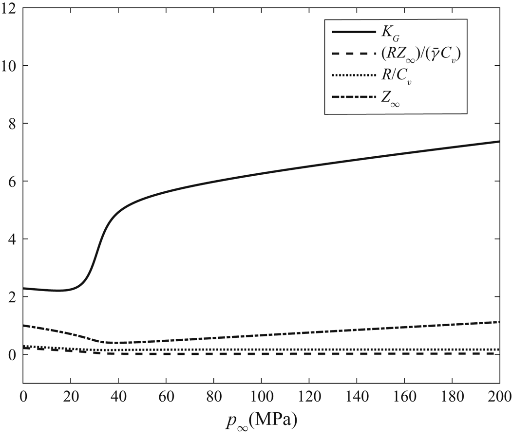
Figure 16. Change of  $K_G$,
  $(RZ_\infty )/(\bar {\gamma } C_v)$,
  $R/C_v$ and
  $Z_\infty$ with
  $p_\infty$ at a fixed
  $T_\infty =700$ K.
Moreover, our computations show that, when  $M_{\infty }=0.8$,
  $\epsilon =0.12$ and
  $\varTheta =0$, the flow exhibits unsteadiness and instability and does not converge to a steady state solution for flow thermodynamic conditions with
  $K_G> 3.2$. In such situations, the shock wave becomes longer and stronger and is pushed downstream to the trailing edge of the airfoil, but exhibits oscillations around the trailing edge.
The variation of  $K_G$ with an increase of
  $T_\infty$ at a fixed
  $p_\infty$ is depicted in figure 17. For flows with
  $p_\infty \leqslant p_c$, where
  $p_c$ is the critical pressure,
  $K_G$ increases with an increase of
  $T_\infty$ above saturation temperature, and approaches the perfect-gas
  $K_G$ (
 ${=}2.33$). For flows with
  $p_\infty > p_c$, as
  $T_\infty$ is increased from 300 K,
  $K_G$ decreases rapidly from high values (
 ${>}10$) until the flow attains the critical entropy value (
 $s=s_c$). At this temperature, the graph of
  $K_G$ versus
  $T_\infty$ shows an inflection point. Upon further increasing
  $T_\infty$,
  $K_G$ decreases gradually and approaches the perfect-gas value of
  $K_G$. At very high temperatures, real-gas effects on the thermodynamics are negligible and
  $K_G= 2.33$ irrespective of the upstream pressure. These variations in
  $K_G$ affect the transonic flow behaviour around an airfoil, as has been demonstrated in §§ 5.1–5.5.
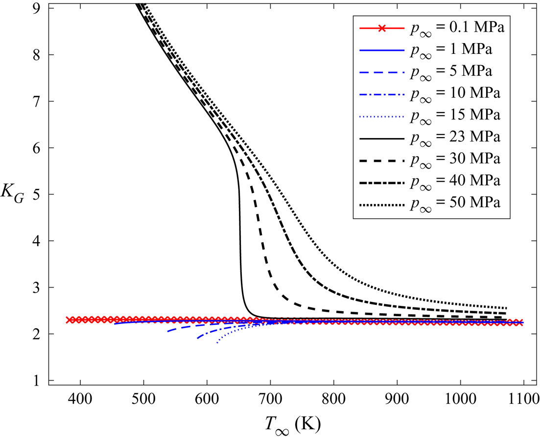
Figure 17. Thermodynamic similarity parameter  $K_G$ as a function of
  $T_\infty$ for various values of
  $p_\infty$.
Figure 18 shows the variation of  $K_G$ computed from the different gas models at a fixed free-stream temperature of
  $T_\infty =700$ K and free-stream pressure varying from low subcritical values to high supercritical values. Results of the virial gas model are not plotted as the model is highly inaccurate in the thermodynamic high supercritical regime. As pressure increases to high supercritical values at a given temperature, the difference between the
  $K_G$ values from the Redlich–Kwong gas model and van der Waals gas model becomes increasingly significant, even though the less accurate model reproduces the qualitative behaviour of the change of
  $K_G$ with
  $p_\infty$. Figure 19 shows the variation of
  $K_G$ computed from the different gas models at a fixed free-stream pressure of
  $p_\infty =40$ MPa and free-stream temperature varying from low subcritical values to high supercritical values. The virial gas model fails to capture the qualitative behaviour of the change of
  $K_G$ at supercritical pressure. The difference between the values of
  $K_G$ from the Redlich–Kwong and van der Waals gas models increases until the critical temperature (
 $T_c$) and decreases beyond that. The effects of thermodynamic modelling using the described models at a fixed supercritical free-stream pressure become greater as free-stream temperature approaches
  $T_c$, and the trend reverses as
  $T_\infty$ is increased beyond
  $T_c$.
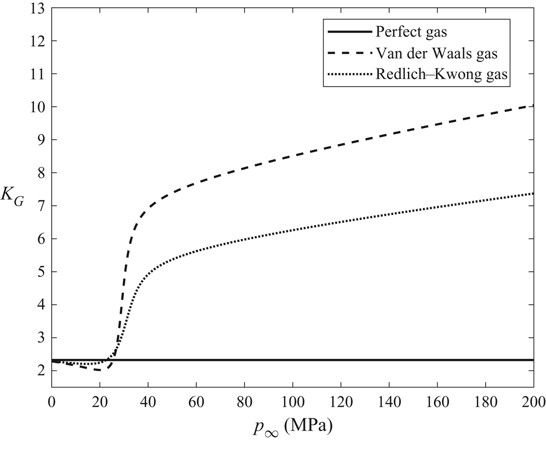
Figure 18. Thermodynamic similarity parameter  $K_G$ as a function of
  $p_\infty$ at
  $T_\infty =700$ K for different gas models.
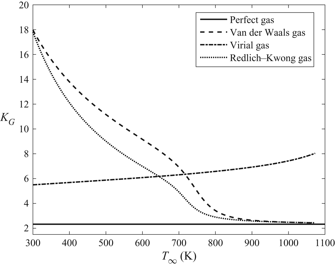
Figure 19. Thermodynamic similarity parameter  $K_G$ as a function of
  $T_\infty$ at
  $p_\infty =40$ MPa for different gas models.
6.2. Similarity between various equation of state TSD models
Similarity between TSD models derived using various gas equations of state at fixed values of upstream thermodynamic conditions ( $p_\infty$ and
  $T_\infty$) can be demonstrated with an example flow problem. The solution of a flow problem at a given
  $M_{\infty 1}$ around a thin airfoil with thickness ratio
  $\epsilon _1$ (marked as case 1) and flow conditions with
  $K_{G1}$ can be used to determine the solution of another similar flow problem (marked as case 2) with a different set of values of
  $M_{\infty 2}$,
  $\epsilon _2$ and
  $K_{G2}$ such that
  $K$ and
  $K_G M_\infty ^2$ for both cases are the same, i.e.
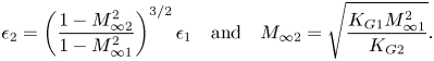 \begin{equation} \epsilon_2= \left(\frac{1-M_{\infty 2}^2}{1-M_{\infty1}^2}\right)^{3/2} \epsilon_1 \quad \textrm{and} \quad M_{\infty 2} = \sqrt{\frac{K_{G1} M_{\infty 1}^2}{K_{G2}}}. \end{equation}
 A steam flow problem is solved around a NACA0012 airfoil ( $\epsilon =0.12$) with
  $T_\infty = 575$ K,
  $p_\infty =5.73$ MPa,
  $M_\infty =0.8$ and
  $\varTheta =0$ using the Redlich–Kwong gas TSD model. The stagnation conditions of upstream fluid for this case are
  $T_0 = 638.9$ K,
  $p_0 = 8.82$ MPa and
  $\varPhi _0 =44.1\,\%$. The solution of this problem is compared with the solution of a steam flow problem around another NACA airfoil with
  $\epsilon = 0.148$ and with the same
  $p_\infty$,
  $T_\infty$ but at
  $M_\infty = 0.766$ using the perfect-gas TSD model. It is also compared with the solution of a steam flow problem around a third NACA airfoil with
  $\epsilon = 0.114$ and with the same
  $p_\infty$,
  $T_\infty$ but at
  $M_\infty = 0.808$ using the van der Waals gas TSD model. Another steam flow problem around a fourth NACA airfoil with
  $\epsilon = 0.091$ is also solved, with the same
  $p_\infty$,
  $T_\infty$ but at
  $M_\infty = 0.837$ using the virial gas TSD model. The
  $K_G$ values for the four cases are given in table 3. Note that
  $K=1.48$ and
  $K_G M_\infty ^2=1.365$ for the four cases are the same at the given conditions. The distributions of scaled pressure coefficient (
 $-C_p/\epsilon ^{2/3}$) on the airfoil surface for the three models were found to overlap, thus demonstrating the similarity between them. As real-gas effects become more dominant (and
  $K_G$ decreases), the upstream flow Mach number should increase and the airfoil thickness should decrease to have a similar flow dynamics as that of a perfect gas.
6.3. Critical upstream flow Mach number as a function of thermodynamic similarity parameter
The relationship of the critical upstream flow Mach number ( $Ma_{c}$) for first appearance of a sonic point on the airfoil surface with the thermodynamic similarity parameter (
 $K_G$) is shown in figure 20. Following detailed computations of various cases, it is found that
  $Ma_c$ decreases nearly linearly as
  $K_G$ is increased. As upstream flow pressure and temperature increase, the real-gas effects become more influential, and
  $K_G$ decreases, see tables 1 and 3 and figures 9 and 10. Increased real-gas effects due to a decrease in
  $K_G$ cause the flow over the airfoil to remain subsonic in nature at higher upstream Mach numbers and the critical upstream Mach number increases. Thereby, a wider range of operational upstream Mach numbers can be found for which pressure drag is zero as the upstream pressure and temperature are increased. Similar results have been reported earlier for flows described by non-classical gas dynamics (
 $\varGamma <0$) (see, e.g. Cramer Reference Cramer1996; Cramer et al. Reference Cramer, Whitlock and Tarkenton1996), even though the increase in
  $Ma_{c}$ is not as significant here as found for flows of fluids with heavier molecular weights such as BZT fluids.
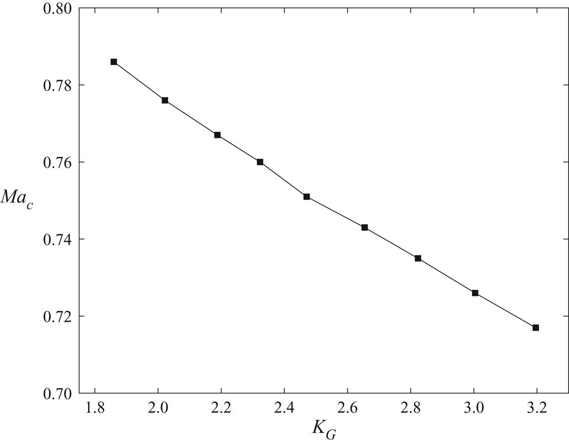
Figure 20. Plot of critical upstream flow Mach number  $Ma_c$ versus thermodynamic similarity parameter
  $K_G$.
7. Conclusions
A small-disturbance model for a steady, two-dimensional, inviscid and transonic flow of a real gas around a thin airfoil is presented. The theoretical approach explores the nonlinear interactions among the near-sonic speed of the flow, the small thickness ratio of the airfoil and the upstream thermodynamic properties of the fluid. The flow thermodynamic behaviour is described by a general equation of state. The asymptotic analysis provides the similarity parameters that govern the flow problem which are the small thickness ratio of the airfoil  $\epsilon$, the transonic similarity parameter
  $K$ and the thermodynamic similarity parameter
  $K_G$ given by (3.5). Information about the thermodynamic modelling of the gas is lumped into one similarity parameter,
  $K_G$, which is related to
  $\varGamma _\infty$ and expressed in terms of partial derivatives of
  $p_\infty$ with respect to
  $T_\infty$ and
  $\rho _\infty$. The flow field may be described by a modified TSD equation (3.9) with relevant far-field conditions and airfoil boundary conditions given by (3.10). Using this general theory, specific TSD models are derived in §§ 3.1, 3.2, 3.3 and 3.4 for flow problems described by the perfect gas, the van der Waals gas, the virial gas and the Redlich–Kwong gas equations of state. The sensitivity of the TSD solution to the thermodynamic modelling of the gas is studied by solving several flow problems in § 5 with different free-stream operating conditions ranging from low subcritical to high supercritical thermodynamic upstream flow states. The theory applies to any working fluid of interest. Steam is considered as an example of the working fluid in the current study. Effects of changes in the free-stream properties of the gas, including supercritical fluid conditions, on the thermodynamic similarity parameter
  $K_G$ and related effects on the flow field are also analysed.
Transonic flow behaviour is found to be independent of the thermodynamic modelling of the gas at low subcritical thermodynamic conditions (§ 5.2). However, at near-critical and supercritical thermodynamic conditions, transonic flow behaviour is significantly sensitive to the thermodynamic modelling of the gas (§§ 5.3 and 5.4). Increasing upstream temperature at fixed upstream pressure, or increasing upstream pressure at fixed upstream temperature, results in a decrease of  $K_G$ at subcritical conditions. This leads to a reduction in the strength and upstream movement of the shock wave on the airfoil surface, and consequent reduction in wave drag of the airfoil. However, at above critical temperatures and pressures,
  $K_G$ increases and this leads to an increase in the strength and downstream movement of the shock wave on the airfoil surface, and an increase in wave drag of the airfoil. Figures 13–17 provide information about the variation of
  $K_G$ with pressure and temperature at below and above thermodynamic critical properties. Figures 18 and 19 compare the values of
  $K_G$ corresponding to different gas models for various free-stream temperatures and pressures. While the van der Waals gas model captures the qualitative behaviour of
  $K_G$ variation with
  $T_\infty$ and
  $p_\infty$, the difference between its prediction and
  $K_G$ from Redlich–Kwong becomes significant near the thermodynamic critical point.
Moreover, similarity rules (6.1a,b) between flow predictions according to TSD models based on various equations of state could be helpful not only for comparing different thermodynamic models for a given fluid but also for comparing flows of different fluids (possibly governed by different equations of state). As real-gas effects become more dominant (and  $K_G$ decreases), the upstream flow Mach number should increase and the airfoil thickness should decrease to have a similar flow dynamics as that of a perfect gas. In the subcritical operational region, the upstream flow critical Mach number increases and wave drag decreases as the upstream flow thermodynamic state becomes near critical. This is due to a decrease of
  $K_G$ in this region. However, in the supercritical operational region, the critical Mach number decreases and the wave drag increases. This is due to a significant increase of
  $K_G$ in this region.
The theoretical framework developed in this study could be used for conducting more detailed studies of the sensitivity of similarity rules in real-gas transonic potential flows to thermodynamic modelling of the gas in different thermodynamic regimes, including supercritical flows. It could also be applied to answer questions concerning real-gas effects in the higher transonic Mach number range, e.g. for sonic free-stream flow, transonic supersonic flow with a detached shock ahead of the airfoil, etc.
Funding
This research received no specific grant from any funding agency, commercial or not-for-profit sectors.
Declaration of interests
The authors report no conflict of interest.
Author contributions
Z.R. and A.S.V. contributed equally to this work.
Appendix A. Derivation of the TSD equation
Following the approach of Cole & Cook (Reference Cole and Cook1986) and Rusak & Lee (Reference Rusak and Lee2000a), the flow properties of the real gas may be approximated by the following asymptotic expansions after a detailed analysis
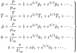 \begin{equation} \left. \begin{gathered} \displaystyle \bar{p} = \frac {p}{p_\infty} = 1+ \epsilon^{2/3}\bar{p}_1 +\epsilon^{4/3}\bar{p}_2 + \cdots ,\\ \displaystyle \bar{T} = \frac {T}{T_\infty} = 1+ \epsilon^{2/3}\bar{T}_1 +\epsilon^{4/3}\bar{T}_2 + \cdots,\\ \displaystyle\bar\rho = \frac {\rho}{\rho_\infty} = 1+ \epsilon^{2/3}\bar\rho_1 +\epsilon^{4/3}\bar\rho_2 + \cdots, \\ \displaystyle\bar{u} =\frac {u}{U_\infty} = 1+ \epsilon^{2/3}\bar{u}_1 +\epsilon^{4/3}\bar{u}_2 + \cdots, \\ \displaystyle\bar{v}= \frac {v}{U_\infty} = \epsilon\bar{v}_1 +\epsilon^{5/3}\bar{v}_2 + \cdots. \\ \end{gathered}\right\} \end{equation}
Substituting (A1) into (2.3)–(2.5), (2.7) and (2.8) results in following equations: from (2.3)
 \begin{equation} \epsilon^ {2/3} (\bar{\rho}_1 +\bar{u}_1)_{\bar{x}} + \epsilon^ {4/3}[(\bar{\rho}_1 \bar{u}_1 +\bar{\rho}_2 +\bar{u}_2 )_{\bar{x}}+\bar{v}_{1\tilde{y}}]+ \cdots = 0, \end{equation}
from (2.4)
 \begin{align} &\epsilon^ {2/3} \left(\frac{ a_\infty^2 M_\infty^2\rho_\infty}{p_\infty} \bar{u}_1 +\bar{p}_1\right)_{\bar{x}}+ \epsilon^ {2/3}\frac{ a_\infty^2 M_\infty^2\rho_\infty}{p_\infty} (\bar\rho_1 +\bar{u}_1)_{\bar{x}} \nonumber\\ &\quad +\epsilon^ {4/3}\left[\left(\frac{ a_\infty^2 M_\infty^2\rho_\infty}{p_\infty}(\bar \rho_2+ 2 \bar{u}_2 + \bar{u}_1^2 + 2\bar \rho_1 \bar{u}_1)+\bar{p}_2\right)_{\bar{x}} + \frac{ a_\infty^2 M_\infty^2\rho_\infty}{p_\infty} \bar{v}_{1 \tilde{y}}\right] \nonumber\\ &\quad +\cdots = 0, \end{align}
from (2.5)
 \begin{equation} \epsilon \left(\bar{p}_{1 \tilde{y}}+ \frac{a_\infty^2 M_\infty^2\rho_\infty}{p_\infty} \bar{v}_{1\bar{x}} \right)+ \cdots = 0, \end{equation}
from (2.7),
 \begin{align} &\epsilon^ {2/3} \left[\bar{p}_1 - \left( \frac{\partial \bar{p}}{\partial \bar{T}} \right)_\infty \bar{T}_1 - \left( \frac{\partial \bar{p}}{\partial \bar \rho}\right)_\infty \bar\rho_1\right]\nonumber\\ &\quad + \epsilon^ {4/3} \left[\bar{p}_2 - \left( \frac{\partial \bar{p}}{\partial \bar{T}}\right)_\infty \bar{T}_2 - \left( \frac{\partial \bar{p}}{\partial \bar \rho} \right)_\infty \bar \rho_2 - \left( \frac{\partial^2 \bar{p}}{\partial \bar \rho \partial \bar{T}}\right)_\infty \bar \rho_1 \bar{T}_1\right. \nonumber\\ &\quad \left.- \frac{1}{2}\left( \frac{\partial^2 \bar{p}}{\partial \bar \rho^2}\right)_\infty\bar \rho_1^2- \frac{1}{2}\left( \frac{\partial^2 \bar{p}}{\partial \bar{T}^2}\right)_\infty\bar{T}_1^2\right] + \cdots = 0, \end{align}
and from (2.8),
 \begin{align} &\epsilon^ {2/3} \left[\bar{T}_1 -\frac{RZ_\infty}{C_v}\bar{b}_\infty \bar{\rho}_1 + \frac{RZ_\infty}{C_v}(\bar{p}_1 -\bar{\rho}_1)+ \bar{\gamma} M_\infty^2 \frac{RZ_\infty}{C_v} \bar{u}_1\right]\nonumber\\ &\quad +\epsilon^ {4/3} \left[\bar{T}_2-\frac{RZ_\infty}{C_v} \left(\bar b_\infty \bar \rho_2 + \left( \frac{\partial \bar{b}}{\partial \bar \rho}\right)_\infty \bar{\rho}_1^2 +\left( \frac{\partial \bar b}{\partial \bar{T}}\right)_\infty \bar{\rho}_1 \bar{T}_1 \right)\right.\nonumber\\ &\quad + \left. \frac{RZ_\infty}{C_v}(\bar{p}_2 - \bar \rho_2 +\bar \rho_1^2-\bar{p}_1 \bar \rho_1) +\bar{\gamma} M_\infty^2 \frac{RZ_\infty}{C_v}\left(\bar{u}_2 + \frac{1}{2} \bar{u}_1^2 \right)\right] + \cdots= 0. \end{align}
In (A6),  $Z_\infty = p_\infty /(\rho _\infty R T_\infty )$ is the compressibility factor of the flow at the upstream state,
  $C_v$ is the specific heat of the gas at constant volume,
  $R = {\mathcal {R}}/\mu$ is the specific gas constant, where
  $\mu$ is the molecular weight of the gas and
  ${\mathcal {R}}$ is the universal gas constant. In (A6), the term
  $b$ and its partial derivatives with respect to density and temperature are
 \begin{equation} \left. \begin{gathered} \displaystyle b = \frac{T}{\rho^2}\frac{\partial p}{\partial T} - \frac{p}{\rho^2},\quad \quad \bar b = b \frac{\rho^2_\infty}{p_\infty}, \\ \displaystyle \left( \frac{\partial \bar b}{\partial \bar \rho}\right)_\infty ={-} 2 \left[\left( \frac{\partial \bar{p}}{\partial \bar{T}}\right)_\infty -1 \right] + \left( \frac{\partial^2 \bar{p}}{\partial \bar{T} \partial \bar \rho}\right)_\infty - \left( \frac{\partial \bar{p}}{\partial \bar \rho}\right)_\infty,\\ \displaystyle \left( \frac{\partial \bar b}{\partial \bar{T}}\right)_\infty =\left( \frac{\partial^2 \bar{p}}{\partial \bar{T}^2}\right)_\infty. \end{gathered}\right\} \end{equation}
Subscript  $\infty$ in the above equations denotes that the partial derivatives are computed at the upstream state. Note that, in (A2) and (A3), the term
  $\epsilon ^ {2/3} (\bar {\rho }_1 +\bar {u}_1)$ may be
  $O(\epsilon ^{4/3})$. Then the leading order,
  $O(\epsilon ^{2/3})$, terms of (A3) give
  $\bar {p}_1+ { a_\infty ^2 M_\infty ^2\rho _\infty \bar {u}_1 }/{p_\infty } = fn(\tilde {y})$. The function
  $fn(\tilde {y})$ should be 0 according to the uniform upstream conditions. Therefore
 \begin{equation} \bar{p}_1 ={-} \frac{ a_\infty^2 M_\infty^2 \rho_\infty}{p_\infty} \bar{u}_1. \end{equation}
Let  $\bar {\gamma } = a_\infty ^2 \rho _\infty /p_\infty$, then
 \begin{equation} \bar{p}_1 ={-} \bar{\gamma} M_\infty^2 \bar{u}_1. \end{equation}
 At the upstream state, the isentropic frozen speed of sound ( $a_\infty$) is
 \begin{equation} a_\infty^2 = \left(\frac{\partial p}{\partial T}\right)^2_{\rho_\infty} \frac{T_\infty}{\rho_\infty^2 C_v} +\left(\frac{\partial p}{\partial \rho}\right)_{T_\infty}=\frac{p_\infty}{\rho_\infty}\left[\frac{RZ_\infty}{C_v}\left(\frac{\partial \bar{p}}{\partial \bar{T}}\right)^2_\infty +\left( \frac{\partial \bar{p}}{\partial \bar \rho}\right)_\infty \right]. \end{equation}
Therefore
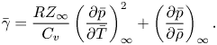 \begin{equation} \bar{\gamma} =\frac{RZ_\infty}{C_v}\left(\frac{\partial \bar{p}}{\partial \bar{T}}\right)^2_\infty + \left( \frac{\partial \bar{p}}{\partial \bar{\rho}}\right)_\infty. \end{equation}
With the assumption of the term  $\epsilon ^ {2/3} (\bar \rho _1 +\bar {u}_1)$ being
  $O(\epsilon ^{4/3})$, (A2) and (A3) together give
 \begin{equation} \bar{p}_2 ={-}\bar{\gamma} M_\infty^2 \bar{u}_2. \end{equation}
From (A9) and the leading order,  $O(\epsilon ^{2/3})$, terms of (A6)
 \begin{equation} \bar{T}_1 = \frac{RZ_\infty}{C_v}(\bar{b}_\infty+1) \bar \rho_1= \frac{RZ_\infty}{C_v}\left(\frac{\partial \bar{p}}{\partial \bar{T}}\right)_\infty\bar{\rho}_1. \end{equation}
 \begin{equation} \bar\rho_1 ={-} M_\infty^2 \bar{u}_1. \end{equation}
As a result,  $\epsilon ^ {2/3} (\bar \rho _1 +\bar {u}_1) = \epsilon ^ {2/3}(1- M_\infty ^2)\bar {u}_1 = \epsilon ^ {4/3} K \bar {u}_1$ which justifies the previous assumption. Using (A9), (A12), (A13) and (A14), (A5) and (A6) to the higher order
  $O(\epsilon ^{4/3})$ gives
 \begin{equation} \bar \rho_2 + M_\infty^2\bar{u}_2 = c M_\infty^2 \bar{u}^2_1, \end{equation}
where
 \begin{align} c &= \frac{2RZ_\infty}{\bar{\gamma} C_v} \left( \frac{\partial \bar{p}}{\partial \bar{T}}\right)^2_\infty + \frac{RZ_\infty}{\bar{\gamma} C_v} \left( \frac{\partial \bar{p}}{\partial \bar{T}}\right)_\infty \left( \frac{\partial \bar{p}}{\partial \bar \rho}\right)_\infty \nonumber\\ &\quad -\frac{RZ_\infty}{\bar{\gamma} C_v} \left( \frac{\partial \bar{p}}{\partial \bar{T}}\right)_\infty \left[\frac{\bar{\gamma}}{2} +1 \right] - \frac{2RZ_\infty}{\bar{\gamma} C_v}\left( \frac{\partial^2 \bar{p}}{\partial \bar \rho \partial \bar{T}}\right)_\infty \left(\frac{\partial \bar{p}}{\partial \bar{T}}\right)_\infty \nonumber\\ &\quad -\frac{1}{2\bar{\gamma}} \left[\left( \frac{\partial^2 \bar{p}}{\partial \bar \rho^2}\right)_\infty +3\left(\frac{RZ_\infty}{C_v}\right)^2 \left( \frac{\partial^2 \bar{p}}{\partial \bar{T}^2}\right)_\infty \left(\frac{\partial \bar{p}}{\partial \bar{T}}\right)^2_\infty \right]. \end{align}
Since  $\bar {\rho }_2 + M_\infty ^2\bar {u}_2 \cong \bar {\rho }_2 +\bar {u}_2$, substituting the value of
  $\bar {\rho }_2 + \bar {u}_2$ from (A15) into (A2) gives
 \begin{equation} \left(\frac{\bar\rho_1 +\bar{u}_1}{\epsilon^{2/3}} + \bar{\rho}_1\bar{u}_1 + c M_\infty^2 \bar{u}^2_1 \right)_{\bar{x}}+\bar{v}_{1\tilde{y}} = 0. \end{equation}
Substituting  $\bar {\rho }_1 = - M_\infty ^2 \bar {u}_1$ and
  $\bar {\rho }_1 +\bar {u}_1 = K \epsilon ^{2/3} \bar {u}_1$ into the above equation
 \begin{equation} \left(K \bar{u}_1 - M_\infty^2 \bar{u}^2_1 + c M_\infty^2 \bar{u}^2_1 \right)_{\bar{x}}+\bar{v}_{1\tilde{y}} = 0, \end{equation}
which can also be written as
 \begin{equation} [K +2(c-1) M_\infty^2 \bar{u}_1]\bar{u}_{1\bar{x}}+\bar{v}_{1\tilde{y}} = 0, \end{equation}
or
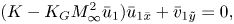 \begin{equation} (K -K_G M_\infty^2 \bar{u}_1)\bar{u}_{1\bar{x}}+\bar{v}_{1\tilde{y}} = 0, \end{equation}
where
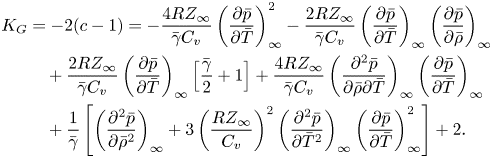 \begin{align} K_G &={-}2(c-1) ={-}\frac{4RZ_\infty}{\bar{\gamma} C_v} \left( \frac{\partial \bar{p}}{\partial \bar{T}}\right)^2_\infty - \frac{2RZ_\infty}{\bar{\gamma} C_v} \left( \frac{\partial \bar{p}}{\partial \bar{T}}\right)_\infty \left( \frac{\partial \bar{p}}{\partial \bar \rho}\right)_\infty \nonumber\\ &\quad +\frac{2RZ_\infty}{\bar{\gamma} C_v} \left( \frac{\partial \bar{p}}{\partial \bar{T}}\right)_\infty \left[\frac{\bar{\gamma}}{2} +1 \right] +\frac{4RZ_\infty}{\bar{\gamma} C_v}\left( \frac{\partial^2 \bar{p}}{\partial \bar{\rho} \partial \bar{T}}\right)_\infty \left(\frac{\partial \bar{p}}{\partial\bar{T}}\right)_\infty \nonumber\\ &\quad +\frac{1}{\bar{\gamma}} \left[ \left( \frac{\partial^2 \bar{p}}{\partial \bar \rho^2}\right)_\infty +3\left(\frac{RZ_\infty}{C_v}\right)^2 \left( \frac{\partial^2 \bar{p}}{\partial \bar{T}^2}\right)_\infty \left(\frac{\partial \bar{p}}{\partial \bar{T}}\right)^2_\infty \right] + 2. \end{align}
Also, from (A4) and (A9), it can be shown that
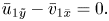 \begin{equation} \bar{u}_{1 \tilde{y}} - \bar{v}_{1 \bar{x}} = 0. \end{equation}
The fundamental derivative of gas dynamics ( $\varGamma$) is a well-known measure of intrinsic gas dynamic nonlinearity and is expressed as
 \begin{equation} \varGamma = 1+ \frac{\rho}{a}\left( \frac{\partial a}{\partial \rho}\right)_s. \end{equation}
The fundamental derivative of gas dynamics at the free-stream state ( $\varGamma _\infty$) therefore is
 \begin{equation} \varGamma_\infty = 1+ \frac{\rho_\infty}{a_\infty}\left( \frac{\partial a_\infty}{\partial \rho_\infty}\right)_{s_\infty}. \end{equation}
Here,  $K_G$ can be related to the value of
  $\varGamma _\infty$. The isentropic frozen speed of sound (
 $a_\infty$) is given by (A10) and
 \begin{equation} \left( \frac{\partial a}{\partial \rho}\right)_{s_\infty} = \left( \frac{\partial a}{\partial T}\right)_{\rho_\infty} \left[ \frac{T_\infty}{\rho^2_\infty C_v} \left( \frac{\partial p}{\partial T}\right)_{\rho_\infty} \right] + \left( \frac{\partial a}{\partial \rho}\right)_{T_\infty}. \end{equation}
The partial derivatives of  $a$ with respect to
  $T$ and
  $\rho$ at the free-stream state are given as
 \begin{align} \left( \frac{\partial a}{\partial T}\right)_{\rho_\infty} = \frac{1}{2a_\infty}\left[ \left( \frac{\partial p}{\partial T}\right)^2_{\rho_\infty} \frac{1}{\rho^2_\infty C_v} + 2 \left( \frac{\partial p}{\partial T}\right)_{\rho_\infty} \left( \frac{\partial^2 p}{\partial T^2}\right)_{\rho_\infty}\frac{T_\infty}{\rho^2_\infty C_v} + \left( \frac{\partial^2 p}{\partial T \partial \rho}\right)_{\infty} \right] \end{align}
and
 \begin{align} \left( \frac{\partial a}{\partial \rho}\right)_{T_\infty} = \frac{1}{2a_\infty}\left[2 \left( \frac{\partial p}{\partial T}\right)_{\rho_\infty} \left( \frac{\partial^2 p}{\partial T \partial \rho}\right)_{\infty} \frac{T_\infty}{\rho^2_\infty C_v} - 2\frac{T_\infty}{\rho^3_\infty C_v}\left( \frac{\partial p}{\partial T}\right)^2_{\rho_\infty} + \left( \frac{\partial^2 p}{\partial \rho^2}\right)_{T_\infty} \right]. \end{align}
Substituting these into (A25) and then substituting the result into (A24) along with (A10) results in
 \begin{align} \varGamma_\infty &={-}\frac{2RZ_\infty}{\bar{\gamma} C_v} \left( \frac{\partial \bar{p}}{\partial \bar{T}}\right)^2_\infty - \frac{RZ_\infty}{\bar{\gamma} C_v} \left( \frac{\partial \bar{p}}{\partial \bar{T}}\right)_\infty \left( \frac{\partial \bar{p}}{\partial \bar \rho}\right)_\infty \nonumber\\ & \quad+\frac{RZ_\infty}{\bar{\gamma} C_v} \left( \frac{\partial \bar{p}}{\partial \bar{T}}\right)_\infty \left[\frac{\bar{\gamma}}{2} +1 \right] +\frac{2RZ_\infty}{\bar{\gamma} C_v}\left( \frac{\partial^2 \bar{p}}{\partial \bar \rho \partial \bar{T}}\right)_\infty \left(\frac{\partial \bar{p}}{\partial \bar{T}}\right)_\infty \nonumber\\ &\quad +\frac{1}{2\bar{\gamma}} \left[ \left( \frac{\partial^2 \bar{p}}{\partial \bar \rho^2}\right)_\infty +3\left(\frac{RZ_\infty}{C_v}\right)^2 \left( \frac{\partial^2 \bar{p}}{\partial \bar{T}^2}\right)_\infty \left(\frac{\partial \bar{p}}{\partial \bar{T}}\right)^2_\infty \right] + 1. \end{align}
Therefore
 \begin{equation} \varGamma_\infty = \frac{K_G}{2}. \end{equation}


