


1 Introduction
Slow viscous flow around a cylinder is a classical problem in fluid mechanics, associated with Stokes’ paradox and its resolution by the inclusion of weak inertial terms in the far field. The analogous problem for non-Newtonian fluids has also played a role in understanding viscoelastic extensional flow (Ultman & Denn Reference Ultman and Denn1971; Harlen Reference Harlen2002) and how a yield stress localizes deformation and provides drag for viscoplastic fluids (Brookes & Whitmore Reference Brookes and Whitmore1969; Adachi & Yoshioka Reference Adachi and Yoshioka1973) and granular materials (Ding, Gravish & Goldman Reference Ding, Gravish and Goldman2011; Hosoi & Goldman Reference Hosoi and Goldman2015). The latter developments connect with soil mechanics and the problem of the critical load required to shift a circular pile through a plastic medium (Randolph & Houlsby Reference Randolph and Houlsby1984; Martin & Randolph Reference Martin and Randolph2006).
The purpose of the present paper is to explore further the viscoplastic version of the problem and analyse flows of yield-stress fluid around cylinders. We have three particular problems in mind. The first is a short reconsideration of the relatively classical problem of the motion of cylinder with a no-slip surface through a viscoplastic medium. This problem has been approached previously using variational methods (Adachi & Yoshioka Reference Adachi and Yoshioka1973), numerical computation (Roquet & Saramito Reference Roquet and Saramito2003; Tokpavi, Magnin & Jay Reference Tokpavi, Magnin and Jay2008; Ozogul, Jay & Magnin Reference Ozogul, Jay and Magnin2015; Chaparian & Frigaard Reference Chaparian and Frigaard2017) and laboratory experiments (Tokpavi et al. Reference Tokpavi, Magnin, Jay and Jossic2009), and has applications to the sedimentation of particles through a viscoplastic medium (Balmforth, Frigaard & Ovarlez Reference Balmforth, Frigaard and Ovarlez2014). In the limit of vanishing flow speeds, one expects that this viscoplastic problem reduces to that for the critical load on a circular pile in an ideal cohesive plastic medium. For that critical load problem, Randolph & Houlsby (Reference Randolph and Houlsby1984) provided an analytical solution using the method of sliplines (the characteristics of the stress field), the no-slip condition corresponding to a fully rough surface. The critical loads found for viscoplastic computations in the limit of no motion do indeed appear to agree with Randolph and Houlsby’s predictions. However, the computed velocity field is not consistent with the slipline solution, containing some unexpected rotating plugs (Tokpavi et al. Reference Tokpavi, Magnin and Jay2008; Chaparian & Frigaard Reference Chaparian and Frigaard2017). This is a concern because the viscoplastic problem is only expected to reduce to one of perfect plasticity outside any boundary layers wherein viscous effects remain important. The residual plugs are attached to such boundary layers at the surface of the cylinder, perhaps reflecting a pervasive viscous effect. We dissect this issue in order to show that the residual plugs disappear in the plastic limit, and thereby demonstrate that there is no conflict with perfect plasticity.
The second problem we address concerns the motion of cylinders whose surface permits some degree of slip. This situation has also been considered in plasticity theory, with Randolph & Houlsby (Reference Randolph and Houlsby1984) searching for the critical load on cylinders with partially rough surfaces. Importantly, the ability of the material to slide over the cylinder demands modifications to the slipline field. Unfortunately, the construction provided by Randolph and Houlsby leads to stress and velocity fields that are inconsistent with one another, implying that their slipline field cannot correspond to the true plastic solution (Murff, Wagner & Randolph Reference Murff, Wagner and Randolph1989; Martin & Randolph Reference Martin and Randolph2006). To shed more light on this issue, we consider viscoplastic flow around cylinders with boundary conditions that allow slip, with a view to approaching the perfectly plastic limit. In so doing, we provide evidence for what is the true plastic solution for these partially rough cylinders. The situation also corresponds to a flow problem wherein sliding is possible or if a thin weakened layer exists sheathing the cylinder, exactly as commonly assumed to explain effective slip (Barnes Reference Barnes1995) and already studied in the context of viscoplastic flow around cylinders (Ozogul et al. Reference Ozogul, Jay and Magnin2015).
Finally, the third problem we consider is the locomotion of cylindrical squirmers in viscoplastic fluid. Squirmers are a popular idealization of swimming micro-organisms that have fixed shape but propel themselves using a prescribed surface velocity field that represents the action of ciliary motion (Lighthill Reference Lighthill1952; Blake Reference Blake1971a ,Reference Blake b ; Pedley Reference Pedley2016). Although most such models are based on spheres, cylindrical squirmers have been considered in Newtonian fluids, to study their interaction with walls or other swimmers (Crowdy & Or Reference Crowdy and Or2010; Clarke, Finn & MacDonald Reference Clarke, Finn and MacDonald2014), or viscoelastic and power-law fluids, to determine their performance in an idealized physiological ambient (Yazdi, Ardekani & Borhan Reference Yazdi, Ardekani and Borhan2014; Ouyang, Lin & Ku Reference Ouyang, Lin and Ku2018). The idealized geometry in these cases allows for a first discussion of the complicating additional physics. Our goal here is to explore how these simplified model swimmers perform in a viscoplastic fluid, following on from related locomotion problems in which a yield stress was demonstrated to dramatically alter the swimming dynamics (Hewitt & Balmforth Reference Hewitt and Balmforth2017, Reference Hewitt and Balmforth2018). Thus, we explore the impact of a yield stress on squirming locomotion, exploiting the results for translating cylinders to understand the exposed flow patterns.
2 Mathematical formulation
Neglecting inertia and gravity, we consider a cylinder of radius
 ${\mathcal{R}}$
moving through an incompressible Bingham fluid (e.g. Balmforth et al. (Reference Balmforth, Frigaard and Ovarlez2014)) with a characteristic speed
${\mathcal{R}}$
moving through an incompressible Bingham fluid (e.g. Balmforth et al. (Reference Balmforth, Frigaard and Ovarlez2014)) with a characteristic speed
 ${\mathcal{U}}$
. To obtain a dimensionless set of equations, we use
${\mathcal{U}}$
. To obtain a dimensionless set of equations, we use
 ${\mathcal{R}}$
and
${\mathcal{R}}$
and
 ${\mathcal{U}}$
to remove the dimensions of length and velocity, respectively. Pressure and stresses are scaled by the characteristic viscous stress
${\mathcal{U}}$
to remove the dimensions of length and velocity, respectively. Pressure and stresses are scaled by the characteristic viscous stress
 $\unicode[STIX]{x1D707}{\mathcal{U}}/{\mathcal{R}}$
where
$\unicode[STIX]{x1D707}{\mathcal{U}}/{\mathcal{R}}$
where
 $\unicode[STIX]{x1D707}$
is the (plastic) viscosity of the fluid. In the polar coordinate system
$\unicode[STIX]{x1D707}$
is the (plastic) viscosity of the fluid. In the polar coordinate system
 $(r,\unicode[STIX]{x1D703})$
with the origin at the centre of the cylinder, the governing equations for the dimensionless fluid velocity
$(r,\unicode[STIX]{x1D703})$
with the origin at the centre of the cylinder, the governing equations for the dimensionless fluid velocity
 $(u(r,\unicode[STIX]{x1D703}),v(r,\unicode[STIX]{x1D703}))$
and pressure
$(u(r,\unicode[STIX]{x1D703}),v(r,\unicode[STIX]{x1D703}))$
and pressure
 $p(r,\unicode[STIX]{x1D703})$
are given by
$p(r,\unicode[STIX]{x1D703})$
are given by
 $$\begin{eqnarray}\displaystyle & \displaystyle \frac{1}{r}\frac{\unicode[STIX]{x2202}}{\unicode[STIX]{x2202}r}(ru)+\frac{1}{r}\frac{\unicode[STIX]{x2202}v}{\unicode[STIX]{x2202}\unicode[STIX]{x1D703}}=0, & \displaystyle\end{eqnarray}$$
 $$\begin{eqnarray}\displaystyle & \displaystyle \frac{\unicode[STIX]{x2202}p}{\unicode[STIX]{x2202}r}=\frac{1}{r}\frac{\unicode[STIX]{x2202}}{\unicode[STIX]{x2202}r}(r\unicode[STIX]{x1D70F}_{rr})+\frac{1}{r}\frac{\unicode[STIX]{x2202}}{\unicode[STIX]{x2202}\unicode[STIX]{x1D703}}\unicode[STIX]{x1D70F}_{r\unicode[STIX]{x1D703}}-\frac{\unicode[STIX]{x1D70F}_{\unicode[STIX]{x1D703}\unicode[STIX]{x1D703}}}{r}, & \displaystyle\end{eqnarray}$$
 $$\begin{eqnarray}\displaystyle & \displaystyle \frac{1}{r}\frac{\unicode[STIX]{x2202}p}{\unicode[STIX]{x2202}\unicode[STIX]{x1D703}}=\frac{1}{r^{2}}\frac{\unicode[STIX]{x2202}}{\unicode[STIX]{x2202}r}(r^{2}\unicode[STIX]{x1D70F}_{r\unicode[STIX]{x1D703}})+\frac{1}{r}\frac{\unicode[STIX]{x2202}}{\unicode[STIX]{x2202}\unicode[STIX]{x1D703}}\unicode[STIX]{x1D70F}_{\unicode[STIX]{x1D703}\unicode[STIX]{x1D703}}, & \displaystyle\end{eqnarray}$$
 $\unicode[STIX]{x1D70F}_{ij}$
is the deviatoric stress tensor. We use the Bingham constitutive law,
$\unicode[STIX]{x1D70F}_{ij}$
is the deviatoric stress tensor. We use the Bingham constitutive law,  $$\begin{eqnarray}\displaystyle \left.\begin{array}{@{}c@{}}\displaystyle \unicode[STIX]{x1D70F}_{ij}=\left(1+\frac{Bi}{\dot{\unicode[STIX]{x1D6FE}}}\right)\dot{\unicode[STIX]{x1D6FE}}_{ij}\quad \text{for }\unicode[STIX]{x1D70F}>Bi,\\ \displaystyle \dot{\unicode[STIX]{x1D6FE}}_{ij}=0\quad \text{for }\unicode[STIX]{x1D70F}\leqslant Bi,\end{array}\right\} & & \displaystyle\end{eqnarray}$$
where
 $$\begin{eqnarray}\displaystyle \{\dot{\unicode[STIX]{x1D6FE}}_{ij}\}=\left(\begin{array}{@{}cc@{}}2u_{r} & v_{r}+(u_{\unicode[STIX]{x1D703}}-v)/r\\ v_{r}+(u_{\unicode[STIX]{x1D703}}-v)/r & 2(v_{\unicode[STIX]{x1D703}}+u)/r\end{array}\right), & & \displaystyle\end{eqnarray}$$
 $\dot{\unicode[STIX]{x1D6FE}}=\sqrt{\frac{1}{2}\sum _{j,k}\dot{\unicode[STIX]{x1D6FE}}_{jk}^{2}}$
and
$\dot{\unicode[STIX]{x1D6FE}}=\sqrt{\frac{1}{2}\sum _{j,k}\dot{\unicode[STIX]{x1D6FE}}_{jk}^{2}}$
and
 $\unicode[STIX]{x1D70F}=\sqrt{\frac{1}{2}\sum _{j,k}\unicode[STIX]{x1D70F}_{jk}^{2}}$
denote the second tensor invariants, and the subscripts
$\unicode[STIX]{x1D70F}=\sqrt{\frac{1}{2}\sum _{j,k}\unicode[STIX]{x1D70F}_{jk}^{2}}$
denote the second tensor invariants, and the subscripts
 $r$
and
$r$
and
 $\unicode[STIX]{x1D703}$
on the velocity components (but not the stress components) denote partial derivatives. The dimensionless yield stress, or Bingham number, is
$\unicode[STIX]{x1D703}$
on the velocity components (but not the stress components) denote partial derivatives. The dimensionless yield stress, or Bingham number, is
 $$\begin{eqnarray}\displaystyle & \displaystyle Bi=\frac{\unicode[STIX]{x1D70F}_{Y}{\mathcal{R}}}{\unicode[STIX]{x1D707}{\mathcal{U}}}. & \displaystyle\end{eqnarray}$$
The drag force on the cylinder in the
 $x$
-direction plays an important role, and is defined by
$x$
-direction plays an important role, and is defined by
 $$\begin{eqnarray}F_{x}=\oint [(\unicode[STIX]{x1D70F}_{rr}-p)\cos \unicode[STIX]{x1D703}-\unicode[STIX]{x1D70F}_{r\unicode[STIX]{x1D703}}\sin \unicode[STIX]{x1D703}]_{r=1}\,\text{d}\unicode[STIX]{x1D703}\equiv \oint [2\unicode[STIX]{x1D70F}_{rr}\cos \unicode[STIX]{x1D703}+(r\unicode[STIX]{x1D70F}_{r\unicode[STIX]{x1D703}})_{r}\sin \unicode[STIX]{x1D703}]_{r=1}\,\text{d}\unicode[STIX]{x1D703}.\end{eqnarray}$$
The plastic drag coefficient
 $C_{d}$
is related to this force by
$C_{d}$
is related to this force by
 $C_{d}=-F_{x}/(2Bi)$
. Although this coefficient is strictly only relevant in the plastic limit
$C_{d}=-F_{x}/(2Bi)$
. Although this coefficient is strictly only relevant in the plastic limit
 $Bi\gg 1$
, the implied rescaling of
$Bi\gg 1$
, the implied rescaling of
 $F_{x}$
is convenient for a wider range of
$F_{x}$
is convenient for a wider range of
 $Bi$
, leading us to use it as a measure of the drag for more general parameter settings.
$Bi$
, leading us to use it as a measure of the drag for more general parameter settings.
2.1 Boundary conditions
2.1.1 Translating cylinder with a rough or no-slip surface
For a no-slip cylinder moving in the
 $x$
-direction with unit speed (i.e. dimensional speed
$x$
-direction with unit speed (i.e. dimensional speed
 ${\mathcal{U}}$
), we impose
${\mathcal{U}}$
), we impose
 $$\begin{eqnarray}\displaystyle (u,v)=(\cos \unicode[STIX]{x1D703},-\sin \unicode[STIX]{x1D703})\quad \text{at }r=1. & & \displaystyle\end{eqnarray}$$
Both velocity conditions cannot be applied in ideal plasticity. Instead, a prescribed normal velocity forces plastic deformation with tangential slip along the boundary of the cylinder. At finite, but large Bingham number, one expects any such slip to become smoothed over viscous boundary layers wherein the shear stress dominates the other stress components. If this turns out to be the case, no-slip is equivalent to the local stress condition
 $|\unicode[STIX]{x1D70F}_{r\unicode[STIX]{x1D703}}|\sim Bi$
, which is the fully rough surface condition used in plasticity theory.
$|\unicode[STIX]{x1D70F}_{r\unicode[STIX]{x1D703}}|\sim Bi$
, which is the fully rough surface condition used in plasticity theory.
2.1.2 Translation with slip
If the surface of the cylinder is partially rough, with a roughness factor
 $\unicode[STIX]{x1D71A}\in [0,1]$
, the boundary condition to be imposed is
$\unicode[STIX]{x1D71A}\in [0,1]$
, the boundary condition to be imposed is
 $$\begin{eqnarray}\displaystyle u=\cos \unicode[STIX]{x1D703}\quad \text{and}\quad \unicode[STIX]{x1D70F}_{r\unicode[STIX]{x1D703}}=\unicode[STIX]{x1D71A}Bi\;\text{sgn}(y)\quad \text{at }r=1 & & \displaystyle\end{eqnarray}$$
(Randolph & Houlsby Reference Randolph and Houlsby1984; Martin & Randolph Reference Martin and Randolph2006); setting
 $\unicode[STIX]{x1D71A}=1$
corresponds to a fully rough cylinder, and
$\unicode[STIX]{x1D71A}=1$
corresponds to a fully rough cylinder, and
 $\unicode[STIX]{x1D71A}=0$
to a perfectly smooth, or free-slip, cylinder. Although it is not necessarily a natural boundary condition for a fluid, the second condition in (2.7) is equivalent to the rate-independent limit of the Mooney-type slip law
$\unicode[STIX]{x1D71A}=0$
to a perfectly smooth, or free-slip, cylinder. Although it is not necessarily a natural boundary condition for a fluid, the second condition in (2.7) is equivalent to the rate-independent limit of the Mooney-type slip law
 $$\begin{eqnarray}\displaystyle v(1,\unicode[STIX]{x1D703})+\sin \unicode[STIX]{x1D703}=A(|\unicode[STIX]{x1D70F}_{r\unicode[STIX]{x1D703}}|-\unicode[STIX]{x1D70F}_{w})^{q}\;\text{sgn}(\unicode[STIX]{x1D70F}_{r\unicode[STIX]{x1D703}}), & & \displaystyle\end{eqnarray}$$
for some parameters
 $A$
,
$A$
,
 $q$
and wall stress threshold
$q$
and wall stress threshold
 $\unicode[STIX]{x1D70F}_{w}=\unicode[STIX]{x1D71A}Bi$
. Such slip laws are common when modelling effective slip due to surface interactions in many suspensions (e.g. Barnes (Reference Barnes1995); see also Ozogul et al. (Reference Ozogul, Jay and Magnin2015)).
$\unicode[STIX]{x1D70F}_{w}=\unicode[STIX]{x1D71A}Bi$
. Such slip laws are common when modelling effective slip due to surface interactions in many suspensions (e.g. Barnes (Reference Barnes1995); see also Ozogul et al. (Reference Ozogul, Jay and Magnin2015)).
2.1.3 Squirming surface motions
For a model squirmer, we again impose the surface velocity, this time in the frame of the cylinder, and select
 ${\mathcal{U}}$
as its characteristic scale. The speed of the cylinder with respect to the ambient fluid then becomes
${\mathcal{U}}$
as its characteristic scale. The speed of the cylinder with respect to the ambient fluid then becomes
 $U_{s}$
. We consider purely tangential squirming motions and set
$U_{s}$
. We consider purely tangential squirming motions and set
 $$\begin{eqnarray}\displaystyle (u,v)=(U_{s}\cos \unicode[STIX]{x1D703},V_{p}(\unicode[STIX]{x1D703})-U_{s}\sin \unicode[STIX]{x1D703})\quad \text{at }r=1, & & \displaystyle\end{eqnarray}$$
where
 $(0,V_{p})$
represents the prescribed surface velocity. For specific examples, we adopt previously employed models of treadmilling cilia given by
$(0,V_{p})$
represents the prescribed surface velocity. For specific examples, we adopt previously employed models of treadmilling cilia given by
 $$\begin{eqnarray}\displaystyle V_{p}(\unicode[STIX]{x1D703})=\sin n\unicode[STIX]{x1D703}+a\sin m\unicode[STIX]{x1D703}, & & \displaystyle\end{eqnarray}$$
with integers
 $n$
and
$n$
and
 $m\neq 1$
. Notable conventional models include the simplest case, with
$m\neq 1$
. Notable conventional models include the simplest case, with
 $(n,a)=(1,0)$
, or employ
$(n,a)=(1,0)$
, or employ
 $(n,m)=(1,2)$
with
$(n,m)=(1,2)$
with
 $a<0$
giving a ‘pusher’ and
$a<0$
giving a ‘pusher’ and
 $a>0$
a ‘puller’ (based on the distribution of
$a>0$
a ‘puller’ (based on the distribution of
 $V_{p}(\unicode[STIX]{x1D703})$
). Note that, although one can generate solutions for any
$V_{p}(\unicode[STIX]{x1D703})$
). Note that, although one can generate solutions for any
 $U_{s}$
, the swimming speed of a free locomotor is set by the requirement that the net force on the cylinder in the
$U_{s}$
, the swimming speed of a free locomotor is set by the requirement that the net force on the cylinder in the
 $x$
-direction should vanish; i.e.
$x$
-direction should vanish; i.e.
 $F_{x}=0$
in (2.5).
$F_{x}=0$
in (2.5).
Finally, we also consider a limited number of examples in which we replace (2.9) with a squirming motion normal to the cylinder surface,
 $$\begin{eqnarray}\left.(u,v)\right|_{r=1}=(U_{s}\cos \unicode[STIX]{x1D703}-U_{p}(\unicode[STIX]{x1D703}),-U_{s}\sin \unicode[STIX]{x1D703}),\quad \text{with }U_{p}=\cos n\unicode[STIX]{x1D703}+a\cos m\unicode[STIX]{x1D703}.\end{eqnarray}$$
Although Blake also considered normal surface velocities, he took these as components of propagating wave-like motions, unlike the steady model in (2.11), which is closer to the propulsion mechanism discussed by Spagnolie & Lauga (Reference Spagnolie and Lauga2010).
2.2 Numerical method
We solve the governing equations using the augmented Lagrangian scheme summarized by Hewitt & Balmforth (Reference Hewitt and Balmforth2017). In brief, after the elimination of the pressure from the momentum equations (2.1b
)–(2.1c
) and the introduction of a stream function
 $\unicode[STIX]{x1D713}(r,\unicode[STIX]{x1D703})$
such that
$\unicode[STIX]{x1D713}(r,\unicode[STIX]{x1D703})$
such that
 $$\begin{eqnarray}\displaystyle & \displaystyle (u,v)=\left(\frac{1}{r}\frac{\unicode[STIX]{x2202}\unicode[STIX]{x1D713}}{\unicode[STIX]{x2202}\unicode[STIX]{x1D703}},-\frac{\unicode[STIX]{x2202}\unicode[STIX]{x1D713}}{\unicode[STIX]{x2202}r}\right), & \displaystyle\end{eqnarray}$$
we must solve the biharmonic-like problem
 $$\begin{eqnarray}\displaystyle & \displaystyle \unicode[STIX]{x1D6FB}^{4}\unicode[STIX]{x1D713}=Bi\left[\left(\frac{1}{r}{\displaystyle \frac{\unicode[STIX]{x2202}}{\unicode[STIX]{x2202}r}}r{\displaystyle \frac{\unicode[STIX]{x2202}}{\unicode[STIX]{x2202}r}}+\frac{2}{r}{\displaystyle \frac{\unicode[STIX]{x2202}}{\unicode[STIX]{x2202}r}}-\frac{1}{r^{2}}{\displaystyle \frac{\unicode[STIX]{x2202}^{2}}{\unicode[STIX]{x2202}\unicode[STIX]{x1D703}^{2}}}\right)\frac{\dot{\unicode[STIX]{x1D6FE}}_{r\unicode[STIX]{x1D703}}}{\dot{\unicode[STIX]{x1D6FE}}}-\frac{2}{r}\left({\displaystyle \frac{\unicode[STIX]{x2202}}{\unicode[STIX]{x2202}r}}+\frac{1}{r}\right){\displaystyle \frac{\unicode[STIX]{x2202}}{\unicode[STIX]{x2202}\unicode[STIX]{x1D703}}}\frac{\dot{\unicode[STIX]{x1D6FE}}_{rr}}{\dot{\unicode[STIX]{x1D6FE}}}\right], & \displaystyle\end{eqnarray}$$
over the yielded regions
 $\dot{\unicode[STIX]{x1D6FE}}>0$
. This is achieved by means of an iterative scheme in which one solves, at each step, a linear biharmonic equation over the whole domain (both yielded and plugged) and a nonlinear algebraic problem that incorporates the constitutive law.
$\dot{\unicode[STIX]{x1D6FE}}>0$
. This is achieved by means of an iterative scheme in which one solves, at each step, a linear biharmonic equation over the whole domain (both yielded and plugged) and a nonlinear algebraic problem that incorporates the constitutive law.
We work on the domain
 $0\leqslant \unicode[STIX]{x1D703}\leqslant \unicode[STIX]{x03C0}$
, with symmetry conditions at
$0\leqslant \unicode[STIX]{x1D703}\leqslant \unicode[STIX]{x03C0}$
, with symmetry conditions at
 $\unicode[STIX]{x1D703}=0,\unicode[STIX]{x03C0}$
. The stress invariant decays away from the cylinder, and must eventually fall below the yield stress. We therefore choose a sufficiently large computational domain to contain all the yielded fluid, and set
$\unicode[STIX]{x1D703}=0,\unicode[STIX]{x03C0}$
. The stress invariant decays away from the cylinder, and must eventually fall below the yield stress. We therefore choose a sufficiently large computational domain to contain all the yielded fluid, and set
 $(u,v)=(0,0)$
at the edge. If both velocity components are also specified on the surface of the cylinder, the boundary conditions there can be implemented directly in terms of the stream function and its derivatives. The boundary condition in (2.7b
), however, imposes the shear stress, which is problematic as the iterative solution of (2.13) requires conditions involving the stream function. To surmount this difficulty, we replace (2.7b
) by the condition
$(u,v)=(0,0)$
at the edge. If both velocity components are also specified on the surface of the cylinder, the boundary conditions there can be implemented directly in terms of the stream function and its derivatives. The boundary condition in (2.7b
), however, imposes the shear stress, which is problematic as the iterative solution of (2.13) requires conditions involving the stream function. To surmount this difficulty, we replace (2.7b
) by the condition
 $\dot{\unicode[STIX]{x1D6FE}}_{r\unicode[STIX]{x1D703}}=\unicode[STIX]{x1D71A}\dot{\unicode[STIX]{x1D6FE}}\,\text{sgn}(y)$
at
$\dot{\unicode[STIX]{x1D6FE}}_{r\unicode[STIX]{x1D703}}=\unicode[STIX]{x1D71A}\dot{\unicode[STIX]{x1D6FE}}\,\text{sgn}(y)$
at
 $r=1$
, which reduces to (2.7b
) where the fluid surface is yielded. If, however, the boundary is plugged, the two conditions are not equivalent. To avoid this inconsistency, in the corresponding computations we used a common regularized constitutive model
$r=1$
, which reduces to (2.7b
) where the fluid surface is yielded. If, however, the boundary is plugged, the two conditions are not equivalent. To avoid this inconsistency, in the corresponding computations we used a common regularized constitutive model
 $\unicode[STIX]{x1D70F}_{ij}=\dot{\unicode[STIX]{x1D6FE}}_{ij}[1+\dot{\unicode[STIX]{x1D6FE}}^{-1}Bi(1-e^{-m\dot{\unicode[STIX]{x1D6FE}}})]$
, which reproduces the Bingham law in (2.2) for
$\unicode[STIX]{x1D70F}_{ij}=\dot{\unicode[STIX]{x1D6FE}}_{ij}[1+\dot{\unicode[STIX]{x1D6FE}}^{-1}Bi(1-e^{-m\dot{\unicode[STIX]{x1D6FE}}})]$
, which reproduces the Bingham law in (2.2) for
 $\dot{\unicode[STIX]{x1D6FE}}\gg m^{-1}$
, with
$\dot{\unicode[STIX]{x1D6FE}}\gg m^{-1}$
, with
 $m=10^{4}$
(this choice of
$m=10^{4}$
(this choice of
 $m$
was sufficiently high that the solutions match those for the unregularized law over the yielded regions, and are insensitive to the precise value of
$m$
was sufficiently high that the solutions match those for the unregularized law over the yielded regions, and are insensitive to the precise value of
 $m$
). Now the fluid is forced to yield everywhere, the boundary is never plugged, and the alternative boundary condition is always equivalent to (2.7b
).
$m$
). Now the fluid is forced to yield everywhere, the boundary is never plugged, and the alternative boundary condition is always equivalent to (2.7b
).
The linear biharmonic equation is solved by exploiting a Fourier sine series in
 $\unicode[STIX]{x1D703}$
, and second-order finite differences in the radial direction. The numerical resolution was chosen to be sufficient to resolve the smallest scales of the problem: the radial grid size was at most
$\unicode[STIX]{x1D703}$
, and second-order finite differences in the radial direction. The numerical resolution was chosen to be sufficient to resolve the smallest scales of the problem: the radial grid size was at most
 $0.003$
, and at least
$0.003$
, and at least
 $512$
Fourier modes in
$512$
Fourier modes in
 $\unicode[STIX]{x1D703}$
were used. In some of our computations at the highest Bingham numbers, we used a stretched grid in the radial direction to enhance the resolution in boundary layers near the cylinder’s surface.
$\unicode[STIX]{x1D703}$
were used. In some of our computations at the highest Bingham numbers, we used a stretched grid in the radial direction to enhance the resolution in boundary layers near the cylinder’s surface.
2.3 Ideal plasticity
In the limit
 $Bi\rightarrow \infty$
, one expects that the viscous stresses become insignificant in comparison to the yield stress outside any boundary layers, implying that yielded material deforms at the yield stress, with
$Bi\rightarrow \infty$
, one expects that the viscous stresses become insignificant in comparison to the yield stress outside any boundary layers, implying that yielded material deforms at the yield stress, with
 $\unicode[STIX]{x1D70F}_{ij}=Bi\dot{\unicode[STIX]{x1D6FE}}_{ij}/\dot{\unicode[STIX]{x1D6FE}}$
. In Cartesian coordinates
$\unicode[STIX]{x1D70F}_{ij}=Bi\dot{\unicode[STIX]{x1D6FE}}_{ij}/\dot{\unicode[STIX]{x1D6FE}}$
. In Cartesian coordinates
 $(x,y)$
, the stress components can then be written in terms of a local slip angle
$(x,y)$
, the stress components can then be written in terms of a local slip angle
 $\unicode[STIX]{x1D717}$
as
$\unicode[STIX]{x1D717}$
as
 $(\unicode[STIX]{x1D70F}_{xx},\unicode[STIX]{x1D70F}_{xy})=Bi(-\sin 2\unicode[STIX]{x1D717},\cos 2\unicode[STIX]{x1D717})$
. Upon substituting the stress components into the momentum equations
$(\unicode[STIX]{x1D70F}_{xx},\unicode[STIX]{x1D70F}_{xy})=Bi(-\sin 2\unicode[STIX]{x1D717},\cos 2\unicode[STIX]{x1D717})$
. Upon substituting the stress components into the momentum equations
 $(\unicode[STIX]{x1D735}\boldsymbol{\cdot }\unicode[STIX]{x1D749}=\unicode[STIX]{x1D735}p)$
, the equations are hyperbolic in
$(\unicode[STIX]{x1D735}\boldsymbol{\cdot }\unicode[STIX]{x1D749}=\unicode[STIX]{x1D735}p)$
, the equations are hyperbolic in
 $p$
and
$p$
and
 $\unicode[STIX]{x1D717}$
with the characteristics of the stress field following the sliplines (Prager & Hodge Reference Prager and Hodge1951),
$\unicode[STIX]{x1D717}$
with the characteristics of the stress field following the sliplines (Prager & Hodge Reference Prager and Hodge1951),
 $$\begin{eqnarray}\displaystyle \unicode[STIX]{x1D6FC}\text{-lines:}\quad \frac{\text{d}y}{\text{d}x}=\tan \unicode[STIX]{x1D717},\quad p+2Bi\unicode[STIX]{x1D717}=\text{constant}, & & \displaystyle\end{eqnarray}$$
 $$\begin{eqnarray}\displaystyle \unicode[STIX]{x1D6FD}\text{-lines:}\quad \frac{\text{d}y}{\text{d}x}=-\cot \unicode[STIX]{x1D717},\quad p-2Bi\unicode[STIX]{x1D717}=\text{constant.} & & \displaystyle\end{eqnarray}$$
The angle
 $\unicode[STIX]{x1D717}$
is the anticlockwise angle of the
$\unicode[STIX]{x1D717}$
is the anticlockwise angle of the
 $\unicode[STIX]{x1D6FC}$
-line as measured from the
$\unicode[STIX]{x1D6FC}$
-line as measured from the
 $x$
-axis. The sliplines are a set of mutually orthogonal lines along which the shear stress is the maximum and the normal stresses are zero. In other words, if
$x$
-axis. The sliplines are a set of mutually orthogonal lines along which the shear stress is the maximum and the normal stresses are zero. In other words, if
 $\unicode[STIX]{x1D64D}(\unicode[STIX]{x1D717})$
denotes the rotation matrix, then,
$\unicode[STIX]{x1D64D}(\unicode[STIX]{x1D717})$
denotes the rotation matrix, then,
 $$\begin{eqnarray}\displaystyle & \displaystyle \unicode[STIX]{x1D64D}(\unicode[STIX]{x1D717})\unicode[STIX]{x1D749}\unicode[STIX]{x1D64D}(\unicode[STIX]{x1D717})^{\text{T}}=\left[\begin{array}{@{}cc@{}}0 & \pm Bi\\ \pm Bi & 0\end{array}\right]. & \displaystyle\end{eqnarray}$$
The components of the velocity field along the sliplines
 $(u_{\unicode[STIX]{x1D6FC}},u_{\unicode[STIX]{x1D6FD}})$
satisfy
$(u_{\unicode[STIX]{x1D6FC}},u_{\unicode[STIX]{x1D6FD}})$
satisfy
 $$\begin{eqnarray}\displaystyle & \displaystyle \frac{\unicode[STIX]{x2202}u_{\unicode[STIX]{x1D6FC}}}{\unicode[STIX]{x2202}s_{\unicode[STIX]{x1D6FC}}}=\frac{\unicode[STIX]{x2202}u_{\unicode[STIX]{x1D6FD}}}{\unicode[STIX]{x2202}s_{\unicode[STIX]{x1D6FD}}}=0, & \displaystyle\end{eqnarray}$$
where
 $s_{\unicode[STIX]{x1D6FC}}$
and
$s_{\unicode[STIX]{x1D6FC}}$
and
 $s_{\unicode[STIX]{x1D6FD}}$
are the arclengths along the respective sliplines. That is, the component of the velocity directed along a particular slipline must be constant.
$s_{\unicode[STIX]{x1D6FD}}$
are the arclengths along the respective sliplines. That is, the component of the velocity directed along a particular slipline must be constant.
The plasticity problem can also be formulated in variational terms to establish the following two useful results (Prager & Hodge Reference Prager and Hodge1951): first, if the velocity field is not simultaneously calculated, slipline fields that satisfy (2.14) and (2.15), together with any stress boundary conditions, constrain the true solution by providing strict lower bounds on the drag force on the cylinder. Second, trial velocity fields that satisfy the surface velocity and incompressibility conditions, but not the stress relations, place upper bounds on the drag force (given that the associated dissipation rate must balance the power input required to overcome the drag). Such upper bounds can be improved by posing trial velocity fields guided by the slipline fields. Indeed, if the lower and upper bounds then match, the stress and the velocity fields must correspond to those of the actual solution. Note that, in the slipline stress analysis, one must further demonstrate that there is an admissible stress distribution inside any rigid plugs that satisfies both the force balance equations and yield criterion (
 $\unicode[STIX]{x1D70F}<Bi$
).
$\unicode[STIX]{x1D70F}<Bi$
).
Randolph & Houlsby (Reference Randolph and Houlsby1984) exploited these bounding principles for a fully rough cylinder driven through a perfectly plastic medium. In particular, they constructed a slipline solution and a matching velocity field for which the upper and lower bounds agreed. They further showed that an admissible stress distribution could be found for all the unyielded regions. Hence, their construction provides the true plastic solution. For partially rough cylinders, however, their trial velocity field was not consistent with the slipline solution over part of the yielded region, and the correct computation of the upper bound leaves a mismatch with the lower bound (Murff et al. Reference Murff, Wagner and Randolph1989). This led Martin & Randolph (Reference Martin and Randolph2006) to suggest an alternative trial velocity field, associated with a different slipline solution, that lay closer to, but not coincident with, the lower bound. The true solution for partially rough cylinders has therefore not been previously identified.
3 Revisiting flow around a no-slip cylinder
In this section, we analyse the viscoplastic flow around a no-slip or fully rough cylinder, focussing on high Bingham number. Figure 1 shows a numerical solution for
 $Bi=2^{14}$
. Plotted is the strain rate, with the regions shaded black corresponding to the plugs, together with Randolph and Houlsby’s slipline solution. Three types of plugs appear in the numerical solution, as found previously (Roquet & Saramito Reference Roquet and Saramito2003; Tokpavi et al.
Reference Tokpavi, Magnin and Jay2008; Chaparian & Frigaard Reference Chaparian and Frigaard2017): first, the ambient medium plugs up sufficiently far from the cylinder to localize the flow. Second, triangular plugs are attached to the front and back of the cylinder. Finally, two plugs with almost semi-circular shape rotate rigidly near the top and bottom of the cylinder. Only the first two types of plugs feature in the perfectly plastic solution; the rigidly rotating plugs lie in the region of perfectly plastic deformation in the slipline solution where there is always shear.
$Bi=2^{14}$
. Plotted is the strain rate, with the regions shaded black corresponding to the plugs, together with Randolph and Houlsby’s slipline solution. Three types of plugs appear in the numerical solution, as found previously (Roquet & Saramito Reference Roquet and Saramito2003; Tokpavi et al.
Reference Tokpavi, Magnin and Jay2008; Chaparian & Frigaard Reference Chaparian and Frigaard2017): first, the ambient medium plugs up sufficiently far from the cylinder to localize the flow. Second, triangular plugs are attached to the front and back of the cylinder. Finally, two plugs with almost semi-circular shape rotate rigidly near the top and bottom of the cylinder. Only the first two types of plugs feature in the perfectly plastic solution; the rigidly rotating plugs lie in the region of perfectly plastic deformation in the slipline solution where there is always shear.

Figure 1. Comparison of the numerical solution and the slipline pattern for a fully rough cylinder. (a) Shows a density plot of
 $\log _{10}(\dot{\unicode[STIX]{x1D6FE}})$
from the numerical solution for
$\log _{10}(\dot{\unicode[STIX]{x1D6FE}})$
from the numerical solution for
 $Bi=2^{14}$
, together with sample streamlines (blue). (b) Shows the
$Bi=2^{14}$
, together with sample streamlines (blue). (b) Shows the
 $\unicode[STIX]{x1D6FC}$
-lines (red) and
$\unicode[STIX]{x1D6FC}$
-lines (red) and
 $\unicode[STIX]{x1D6FD}$
-lines (blue) of the plastic solution, with the centred fans shaded white and the region of involutes shaded green. In both cases, the plugs are shaded black. Arrows indicate the direction of motion of the cylinder.
$\unicode[STIX]{x1D6FD}$
-lines (blue) of the plastic solution, with the centred fans shaded white and the region of involutes shaded green. In both cases, the plugs are shaded black. Arrows indicate the direction of motion of the cylinder.
3.1 Randolph and Houlsby’s slipline solution
In detail and for the upper half of the solution, the slipline pattern (figure 1
b) consists of a semi-circular centred fan at the top of the cylinder with centre
 $A$
at
$A$
at
 $(0,1)$
and radius
$(0,1)$
and radius
 $1+\unicode[STIX]{x03C0}/4$
. The
$1+\unicode[STIX]{x03C0}/4$
. The
 $\unicode[STIX]{x1D6FD}$
-lines form the spokes and the
$\unicode[STIX]{x1D6FD}$
-lines form the spokes and the
 $\unicode[STIX]{x1D6FC}$
-lines form the circular arcs. The
$\unicode[STIX]{x1D6FC}$
-lines form the circular arcs. The
 $\unicode[STIX]{x1D6FC}$
-lines are continued below the line
$\unicode[STIX]{x1D6FC}$
-lines are continued below the line
 $AD$
by the involutes of the cylinder, and the
$AD$
by the involutes of the cylinder, and the
 $\unicode[STIX]{x1D6FD}$
-lines become tangents. The construction of the involutes ensures that the stress field satisfies the fully rough boundary condition,
$\unicode[STIX]{x1D6FD}$
-lines become tangents. The construction of the involutes ensures that the stress field satisfies the fully rough boundary condition,
 $\unicode[STIX]{x1D70F}_{r\unicode[STIX]{x1D703}}=Bi$
, on the cylinder surface. The limiting
$\unicode[STIX]{x1D70F}_{r\unicode[STIX]{x1D703}}=Bi$
, on the cylinder surface. The limiting
 $\unicode[STIX]{x1D6FD}$
-lines
$\unicode[STIX]{x1D6FD}$
-lines
 $BC$
and
$BC$
and
 $B^{\prime }C^{\prime }$
intersect the
$B^{\prime }C^{\prime }$
intersect the
 $x$
-axis at
$x$
-axis at
 $45^{\circ }$
, as demanded by symmetry, which isolates the triangular plugs capping the front and back of the cylinder. The
$45^{\circ }$
, as demanded by symmetry, which isolates the triangular plugs capping the front and back of the cylinder. The
 $\unicode[STIX]{x1D6FC}$
-line
$\unicode[STIX]{x1D6FC}$
-line
 $CDGD^{\prime }C^{\prime }$
determines the outermost yield surface.
$CDGD^{\prime }C^{\prime }$
determines the outermost yield surface.
The velocity field associated with the slipline pattern is directed purely along the
 $\unicode[STIX]{x1D6FC}$
-lines (and so, in this case, the streamlines are
$\unicode[STIX]{x1D6FC}$
-lines (and so, in this case, the streamlines are
 $\unicode[STIX]{x1D6FC}$
-lines): the involutes beginning along
$\unicode[STIX]{x1D6FC}$
-lines): the involutes beginning along
 $BC$
have
$BC$
have
 $v_{\unicode[STIX]{x1D6FC}}=1/\sqrt{2}$
, whereas those that begin at the cylinder along
$v_{\unicode[STIX]{x1D6FC}}=1/\sqrt{2}$
, whereas those that begin at the cylinder along
 $AB$
have
$AB$
have
 $v_{\unicode[STIX]{x1D6FC}}=\cos \unicode[STIX]{x1D703}$
. At the base of both sets of sliplines, there is a velocity jump tangential to
$v_{\unicode[STIX]{x1D6FC}}=\cos \unicode[STIX]{x1D703}$
. At the base of both sets of sliplines, there is a velocity jump tangential to
 $ABC$
. Similarly, along the outermost yield surface
$ABC$
. Similarly, along the outermost yield surface
 $CDGD^{\prime }C^{\prime }$
, another velocity jump arises. In the viscoplastic computation, all these discontinuities become broadened into thin boundary layers with enhanced shear rate (see figure 1(a), or figure 14 in appendix A, for a magnification of the boundary layer attached to the cylinder). The thickness of these layers is expected to scale with either
$CDGD^{\prime }C^{\prime }$
, another velocity jump arises. In the viscoplastic computation, all these discontinuities become broadened into thin boundary layers with enhanced shear rate (see figure 1(a), or figure 14 in appendix A, for a magnification of the boundary layer attached to the cylinder). The thickness of these layers is expected to scale with either
 $Bi^{-1/3}$
or
$Bi^{-1/3}$
or
 $Bi^{-1/2}$
(Balmforth et al.
Reference Balmforth, Craster, Hewitt, Hormozi and Maleki2017), but otherwise they leave no enduring viscous disfigurement of the plastic solution.
$Bi^{-1/2}$
(Balmforth et al.
Reference Balmforth, Craster, Hewitt, Hormozi and Maleki2017), but otherwise they leave no enduring viscous disfigurement of the plastic solution.
Along the
 $\unicode[STIX]{x1D6FD}$
-lines, the Riemann invariant is
$\unicode[STIX]{x1D6FD}$
-lines, the Riemann invariant is
 $p-2Bi\unicode[STIX]{x1D717}$
. If we set
$p-2Bi\unicode[STIX]{x1D717}$
. If we set
 $p=0$
along the vertical symmetry line at
$p=0$
along the vertical symmetry line at
 $x=0$
, this implies
$x=0$
, this implies
 $p=2Bi(\unicode[STIX]{x03C0}-\unicode[STIX]{x1D717})$
throughout the deformed region, and so the pressure on the surface of the cylinder is given by
$p=2Bi(\unicode[STIX]{x03C0}-\unicode[STIX]{x1D717})$
throughout the deformed region, and so the pressure on the surface of the cylinder is given by
 $$\begin{eqnarray}\displaystyle p(1,\unicode[STIX]{x1D703})=\left\{\begin{array}{@{}ll@{}}2Bi(\unicode[STIX]{x03C0}-\unicode[STIX]{x1D703}), & \unicode[STIX]{x03C0}/4<\unicode[STIX]{x1D703}<\unicode[STIX]{x03C0}/2,\\ 2Bi(\unicode[STIX]{x03C0}-\unicode[STIX]{x1D703})-2Bi\unicode[STIX]{x03C0}, & \unicode[STIX]{x03C0}/2<\unicode[STIX]{x1D703}<3\unicode[STIX]{x03C0}/4,\end{array}\right. & & \displaystyle\end{eqnarray}$$
which jumps by
 $2\unicode[STIX]{x03C0}Bi$
at the centre of the fan.
$2\unicode[STIX]{x03C0}Bi$
at the centre of the fan.
With the stresses implied by the slipline pattern, we may integrate over the contour
 $CBAB^{\prime }C^{\prime }$
to determine the net horizontal force on the upper half of the cylinder
$CBAB^{\prime }C^{\prime }$
to determine the net horizontal force on the upper half of the cylinder
 $F_{x}$
(although the stress field is not prescribed over the plugs, the net force on these regions must vanish, and so the horizontal force along
$F_{x}$
(although the stress field is not prescribed over the plugs, the net force on these regions must vanish, and so the horizontal force along
 $BC$
or
$BC$
or
 $B^{\prime }C^{\prime }$
must equal that along the corresponding plugged section of the cylinder’s surface). We then find the drag coefficient (Randolph & Houlsby Reference Randolph and Houlsby1984),
$B^{\prime }C^{\prime }$
must equal that along the corresponding plugged section of the cylinder’s surface). We then find the drag coefficient (Randolph & Houlsby Reference Randolph and Houlsby1984),
 $$\begin{eqnarray}\displaystyle & \displaystyle C_{d}=-\frac{F_{x}}{2Bi}=2(\unicode[STIX]{x03C0}+2\sqrt{2})\simeq 11.94. & \displaystyle\end{eqnarray}$$
3.2 The residual plugs
The rotating plugs of the viscoplastic computation in figure 1(a) are centred at the fans of the slipline solution and are attached to the viscous boundary layer buffering the cylinder surface. Since the viscous stress is prominent in that boundary layer, the question arises as to how the pressure jump at the centre of the fan becomes smoothed and whether this prompts a permanent adjustment of the slipline solution that explains the rotating plugs. Indeed, both Tokpavi et al. (Reference Tokpavi, Magnin and Jay2008) and Chaparian & Frigaard (Reference Chaparian and Frigaard2017) have suggested that these features are permanent for
 $Bi\rightarrow \infty$
. Such a conclusion is problematic as it implies that the viscoplastic theory does not converge to perfect plasticity.
$Bi\rightarrow \infty$
. Such a conclusion is problematic as it implies that the viscoplastic theory does not converge to perfect plasticity.
The current computations suggest an alternative perspective: the rotating plugs correspond to a persistent effect that arises from the pressure discontinuity of the slipline solution at the centre of the centred fans. Because fluid flows through the pressure gradient here, the discontinuity must necessarily become smoothed by viscous stresses over a narrow window of angles
 $\unicode[STIX]{x1D703}$
surrounding
$\unicode[STIX]{x1D703}$
surrounding
 $A$
. The angular scale of this smoothing region turns out to be relatively wide (in comparison to the viscous boundary layers), scaling very weakly with
$A$
. The angular scale of this smoothing region turns out to be relatively wide (in comparison to the viscous boundary layers), scaling very weakly with
 $Bi$
; see figures 2 and 3(d). Moreover, to accommodate the smoothing of the pressure over this scale (which is too wide to allow any viscous adjustments), the overlying plastic flow must plug up, thereby creating the persistent features. Crucially, the size of the plug therefore asymptotically decreases to zero, albeit extremely slowly, as
$Bi$
; see figures 2 and 3(d). Moreover, to accommodate the smoothing of the pressure over this scale (which is too wide to allow any viscous adjustments), the overlying plastic flow must plug up, thereby creating the persistent features. Crucially, the size of the plug therefore asymptotically decreases to zero, albeit extremely slowly, as
 $Bi\rightarrow \infty$
(see figure 3
a; we find, in particular, that the radius decreases like
$Bi\rightarrow \infty$
(see figure 3
a; we find, in particular, that the radius decreases like
 $Bi^{-3/28}$
). Consequently, the drag coefficient should approach the prediction in (3.2) for
$Bi^{-3/28}$
). Consequently, the drag coefficient should approach the prediction in (3.2) for
 $Bi\rightarrow \infty$
, as illustrated by the numerical results (figure 4
a).
$Bi\rightarrow \infty$
, as illustrated by the numerical results (figure 4
a).

Figure 2. Pressure variation over the cylinder scaled by
 $Bi$
, for the Bingham numbers indicated. The dashed line corresponds to the pressure of the slipline solution given by (3.1). The inset shows
$Bi$
, for the Bingham numbers indicated. The dashed line corresponds to the pressure of the slipline solution given by (3.1). The inset shows
 $p/Bi$
against
$p/Bi$
against
 $(\unicode[STIX]{x1D703}-\unicode[STIX]{x03C0}/2)Bi^{1/7}$
.
$(\unicode[STIX]{x1D703}-\unicode[STIX]{x03C0}/2)Bi^{1/7}$
.

Figure 3. Scaling data for the residual rotating plug against
 $Bi$
, showing (a) the plug radius
$Bi$
, showing (a) the plug radius
 $y_{p}-1$
(where
$y_{p}-1$
(where
 $(0,y_{p})$
is the the top of the plug), (b) the rotation rate
$(0,y_{p})$
is the the top of the plug), (b) the rotation rate
 $\unicode[STIX]{x1D714}$
, (c) the boundary layer thickness at
$\unicode[STIX]{x1D714}$
, (c) the boundary layer thickness at
 $\unicode[STIX]{x1D703}=\frac{1}{2}\unicode[STIX]{x03C0}$
and
$\unicode[STIX]{x1D703}=\frac{1}{2}\unicode[STIX]{x03C0}$
and
 $\frac{1}{3}\unicode[STIX]{x03C0}$
, and (d) the angular size of the smoothing region, estimated by the location
$\frac{1}{3}\unicode[STIX]{x03C0}$
, and (d) the angular size of the smoothing region, estimated by the location
 $\hat{\unicode[STIX]{x1D703}}_{\ast }$
for which
$\hat{\unicode[STIX]{x1D703}}_{\ast }$
for which
 $p=\frac{1}{2}Bi$
. The dashed lines indicate the expected scalings according to the boundary-layer theory of appendix A.
$p=\frac{1}{2}Bi$
. The dashed lines indicate the expected scalings according to the boundary-layer theory of appendix A.

Figure 4. (a) Drag coefficient
 $C_{d}$
against
$C_{d}$
against
 $Bi$
for computations using a no-slip boundary condition (red circles) or the plastic slip law in (2.7) with
$Bi$
for computations using a no-slip boundary condition (red circles) or the plastic slip law in (2.7) with
 $\unicode[STIX]{x1D71A}=1$
(blue stars). The dashed line shows (3.2). (b) Plots of
$\unicode[STIX]{x1D71A}=1$
(blue stars). The dashed line shows (3.2). (b) Plots of
 $\log _{10}\dot{\unicode[STIX]{x1D6FE}}$
and streamlines for two solutions at
$\log _{10}\dot{\unicode[STIX]{x1D6FE}}$
and streamlines for two solutions at
 $Bi=2^{8}$
; the upper half shows the no-slip cylinder, and the lower half the cylinder with (2.7) and
$Bi=2^{8}$
; the upper half shows the no-slip cylinder, and the lower half the cylinder with (2.7) and
 $\unicode[STIX]{x1D71A}=1$
.
$\unicode[STIX]{x1D71A}=1$
.
A number of other numerical results are shown in figure 3, including the rotation rate of the plug and the thickness of the boundary layer against the cylinder. Notably, directly under the plug, the boundary layer is thinned by the presence of the smoothing region, scaling with
 $Bi^{-4/7}$
. Beyond this region, the boundary layer has a thickness of
$Bi^{-4/7}$
. Beyond this region, the boundary layer has a thickness of
 $O(Bi^{-1/2})$
, as expected from viscoplastic boundary-layer theory (Balmforth et al.
Reference Balmforth, Craster, Hewitt, Hormozi and Maleki2017). The thinner boundary-layer scaling near
$O(Bi^{-1/2})$
, as expected from viscoplastic boundary-layer theory (Balmforth et al.
Reference Balmforth, Craster, Hewitt, Hormozi and Maleki2017). The thinner boundary-layer scaling near
 $A$
is in disagreement with the conclusions of Tokpavi et al. (Reference Tokpavi, Magnin and Jay2008), although the difference between
$A$
is in disagreement with the conclusions of Tokpavi et al. (Reference Tokpavi, Magnin and Jay2008), although the difference between
 $-1/2$
and
$-1/2$
and
 $-4/7$
is small (these authors actually find a scaling of
$-4/7$
is small (these authors actually find a scaling of
 $-0.53$
). A boundary-layer theory in support of the observed scalings and the overall phenomenology of the rotating plug is provided in appendix A.
$-0.53$
). A boundary-layer theory in support of the observed scalings and the overall phenomenology of the rotating plug is provided in appendix A.
A key feature of the boundary-layer theory is that the slowly converging scalings of the rotating plug arise from the interplay between the flow within the boundary layer and the overlying plastic deformation. The important role played by the boundary layer therefore implies that the passage to the plastic limit should be different if that sharp feature is not present. Indeed, when we recompute the solutions using the slip law outlined in § 2.1.2 (with
 $\unicode[STIX]{x1D71A}=1$
, corresponding to a fully rough surface), the boundary layers against the cylinder are removed as all the tangential slip that is required for the adjacent perfectly plastic deformation can be taken up along the boundary itself. No slowly shrinking plugs then appear at the centre of the fans whatsoever and the convergence to the plastic limit is noticeably accelerated (see figure 4).
$\unicode[STIX]{x1D71A}=1$
, corresponding to a fully rough surface), the boundary layers against the cylinder are removed as all the tangential slip that is required for the adjacent perfectly plastic deformation can be taken up along the boundary itself. No slowly shrinking plugs then appear at the centre of the fans whatsoever and the convergence to the plastic limit is noticeably accelerated (see figure 4).
4 Flow past a partially rough cylinder
Numerical solutions for partially rough cylinders, with boundary condition (2.7), are shown in figures 5 and 6. The first of these figures displays strain-rate plots for two sample solutions with different roughness factors
 $\unicode[STIX]{x1D71A}=0$
(free-slip) and
$\unicode[STIX]{x1D71A}=0$
(free-slip) and
 $\unicode[STIX]{x1D71A}=\frac{1}{2}$
. Aside from viscoplastic shear layers that smooth out the velocity jumps, these numerical solutions are very like the slipline solution proposed by Martin & Randolph (Reference Martin and Randolph2006) which are also plotted in the figure and described in more detail below. Notably, the solutions now contain rigidly rotating plugs that are permanent features in the plastic limit
$\unicode[STIX]{x1D71A}=\frac{1}{2}$
. Aside from viscoplastic shear layers that smooth out the velocity jumps, these numerical solutions are very like the slipline solution proposed by Martin & Randolph (Reference Martin and Randolph2006) which are also plotted in the figure and described in more detail below. Notably, the solutions now contain rigidly rotating plugs that are permanent features in the plastic limit
 $Bi\rightarrow \infty$
, and which attach directly onto the sliding cylinder surface.
$Bi\rightarrow \infty$
, and which attach directly onto the sliding cylinder surface.

Figure 5. Numerical solutions showing
 $\log _{10}\dot{\unicode[STIX]{x1D6FE}}$
and streamlines (left) and slipline solutions (right) for (a)
$\log _{10}\dot{\unicode[STIX]{x1D6FE}}$
and streamlines (left) and slipline solutions (right) for (a)
 $\unicode[STIX]{x1D71A}=0$
and (b)
$\unicode[STIX]{x1D71A}=0$
and (b)
 $\unicode[STIX]{x1D71A}=0.5$
, both at
$\unicode[STIX]{x1D71A}=0.5$
, both at
 $Bi=2^{12}$
. The light blue lines on the left indicate streamlines. On the right, the
$Bi=2^{12}$
. The light blue lines on the left indicate streamlines. On the right, the
 $\unicode[STIX]{x1D6FC}$
and
$\unicode[STIX]{x1D6FC}$
and
 $\unicode[STIX]{x1D6FD}$
-lines are plotted in red and blue, respectively, with the plugs shaded grey and the region of involutes shaded green. Also indicated are the angle
$\unicode[STIX]{x1D6FD}$
-lines are plotted in red and blue, respectively, with the plugs shaded grey and the region of involutes shaded green. Also indicated are the angle
 $\unicode[STIX]{x1D6FD}_{2}$
(equal to
$\unicode[STIX]{x1D6FD}_{2}$
(equal to
 $63.0^{\circ }$
in (a) and
$63.0^{\circ }$
in (a) and
 $69.2^{\circ }$
in (b)) and a number of special points in the slipline field. The primed points,
$69.2^{\circ }$
in (b)) and a number of special points in the slipline field. The primed points,
 $B^{\prime }$
to
$B^{\prime }$
to
 $F^{\prime }$
, are the reflections of points,
$F^{\prime }$
, are the reflections of points,
 $B$
to
$B$
to
 $F$
, about the
$F$
, about the
 $y$
-axis.
$y$
-axis.
4.1 The Martin and Randolph slipline solution and upper bound
As for Randolph and Houlsby’s slipline field shown in figure 1, the pattern proposed by Martin & Randolph (Reference Martin and Randolph2006) consists of centred fans and involutes that leave a triangular plug at the front and back of the cylinder. However, the centres of fans are now displaced off the surface and the cores of the fans are replaced by the rigidly rotating plugs. Focussing on the upper right half of the pattern, the fan is centred at point
 $P$
and occupies the region
$P$
and occupies the region
 $EFDGI$
in figure 5. The rotating plug spans
$EFDGI$
in figure 5. The rotating plug spans
 $AEI$
. The involutes that extend the
$AEI$
. The involutes that extend the
 $\unicode[STIX]{x1D6FC}$
-lines from the fan into
$\unicode[STIX]{x1D6FC}$
-lines from the fan into
 $EBCDF$
correspond to
$EBCDF$
correspond to
 $\unicode[STIX]{x1D6FD}$
-lines that are tangent to an inner circle centred at
$\unicode[STIX]{x1D6FD}$
-lines that are tangent to an inner circle centred at
 $O$
with radius
$O$
with radius
 $$\begin{eqnarray}\displaystyle & \displaystyle \unicode[STIX]{x1D706}=\cos \left(\frac{\cos ^{-1}\unicode[STIX]{x1D71A}}{2}\right). & \displaystyle\end{eqnarray}$$
This choice for
 $\unicode[STIX]{x1D706}$
ensures that the
$\unicode[STIX]{x1D706}$
ensures that the
 $\unicode[STIX]{x1D6FC}$
-lines meet the surface of the cylinder at an angle
$\unicode[STIX]{x1D6FC}$
-lines meet the surface of the cylinder at an angle
 $(\unicode[STIX]{x03C0}/4-\unicode[STIX]{x1D6E5}/2)$
, where
$(\unicode[STIX]{x03C0}/4-\unicode[STIX]{x1D6E5}/2)$
, where
 $\unicode[STIX]{x1D6E5}=\sin ^{-1}\unicode[STIX]{x1D71A}$
, in line with the boundary condition (2.7b
) on
$\unicode[STIX]{x1D6E5}=\sin ^{-1}\unicode[STIX]{x1D71A}$
, in line with the boundary condition (2.7b
) on
 $EB$
,
$EB$
,
 $|\unicode[STIX]{x1D70F}_{r\unicode[STIX]{x1D703}}|/Bi=\unicode[STIX]{x1D71A}$
. In other words, the unwrapping of the
$|\unicode[STIX]{x1D70F}_{r\unicode[STIX]{x1D703}}|/Bi=\unicode[STIX]{x1D71A}$
. In other words, the unwrapping of the
 $\unicode[STIX]{x1D6FD}$
-lines from the inner circle ensures that the slip condition is satisfied along the yielded boundary of the cylinder, and follows Randolph and Houlsby’s original generalization of figure 1 for
$\unicode[STIX]{x1D6FD}$
-lines from the inner circle ensures that the slip condition is satisfied along the yielded boundary of the cylinder, and follows Randolph and Houlsby’s original generalization of figure 1 for
 $\unicode[STIX]{x1D71A}<1$
. The main difference between their generalization and the construction of Martin and Randolph is the introduction of the rigidly rotating plugs at the cores of the fans. Such plugs are permitted because any slipline can be taken as a yield surface and the normal velocity across the sliding, unyielded boundary can be made continuous by demanding that the rotation rate of the plugs is
$\unicode[STIX]{x1D71A}<1$
. The main difference between their generalization and the construction of Martin and Randolph is the introduction of the rigidly rotating plugs at the cores of the fans. Such plugs are permitted because any slipline can be taken as a yield surface and the normal velocity across the sliding, unyielded boundary can be made continuous by demanding that the rotation rate of the plugs is
 $\sin \unicode[STIX]{x1D6FD}_{2}/\unicode[STIX]{x1D706}$
, where
$\sin \unicode[STIX]{x1D6FD}_{2}/\unicode[STIX]{x1D706}$
, where
 $\unicode[STIX]{x03C0}-\unicode[STIX]{x1D6FD}_{2}$
dictates the angular extent of the fan (the angle between
$\unicode[STIX]{x03C0}-\unicode[STIX]{x1D6FD}_{2}$
dictates the angular extent of the fan (the angle between
 $IPE$
). The introduction of the plugs then shifts the centre of the fan
$IPE$
). The introduction of the plugs then shifts the centre of the fan
 $P$
so that it lies a vertical distance
$P$
so that it lies a vertical distance
 $\unicode[STIX]{x1D706}/\sin \unicode[STIX]{x1D6FD}_{2}$
above
$\unicode[STIX]{x1D706}/\sin \unicode[STIX]{x1D6FD}_{2}$
above
 $O$
.
$O$
.
Again, the velocity field over the plastic region is prescribed by
 $v_{\unicode[STIX]{x1D6FD}}=0$
and matching
$v_{\unicode[STIX]{x1D6FD}}=0$
and matching
 $v_{\unicode[STIX]{x1D6FC}}$
with the normal velocity to the contour
$v_{\unicode[STIX]{x1D6FC}}$
with the normal velocity to the contour
 $EBC$
. Velocity jumps thereby occur along the
$EBC$
. Velocity jumps thereby occur along the
 $\unicode[STIX]{x1D6FC}$
-lines
$\unicode[STIX]{x1D6FC}$
-lines
 $BFH$
and
$BFH$
and
 $CDG$
, which broaden into the prominent viscoplastic shear layers of the computations in figure 5, and fluid slides along the cylinder boundary
$CDG$
, which broaden into the prominent viscoplastic shear layers of the computations in figure 5, and fluid slides along the cylinder boundary
 $AEB$
.
$AEB$
.

Figure 6. Upper and lower bounds derived from Martin and Randolph’s slipline solution (solid blue and black lines, respectively) for the values of
 $\unicode[STIX]{x1D71A}$
indicated; the circles indicate the minimum of the upper bound, which coincides with the intersection with the lower bound. For
$\unicode[STIX]{x1D71A}$
indicated; the circles indicate the minimum of the upper bound, which coincides with the intersection with the lower bound. For
 $\unicode[STIX]{x1D6FD}_{2}$
less than this minimum, the lower bound exceeds the upper bound and is thus spurious (shown dashed). For
$\unicode[STIX]{x1D6FD}_{2}$
less than this minimum, the lower bound exceeds the upper bound and is thus spurious (shown dashed). For
 $\unicode[STIX]{x1D6FD}_{2}>\frac{1}{2}\unicode[STIX]{x03C0}$
, the velocity and stress fields become inconsistent, as in the original Randolph and Houlsby construction (the corresponding bounds are shown by dotted lines). The red stars show the extrapolated values for
$\unicode[STIX]{x1D6FD}_{2}>\frac{1}{2}\unicode[STIX]{x03C0}$
, the velocity and stress fields become inconsistent, as in the original Randolph and Houlsby construction (the corresponding bounds are shown by dotted lines). The red stars show the extrapolated values for
 $Bi\rightarrow \infty$
of the drag and angle
$Bi\rightarrow \infty$
of the drag and angle
 $\unicode[STIX]{x1D6FD}_{2}$
from numerical computations. For the latter, the rotation rate of the rigid plugs,
$\unicode[STIX]{x1D6FD}_{2}$
from numerical computations. For the latter, the rotation rate of the rigid plugs,
 $\sin \unicode[STIX]{x1D6FD}_{2}/\unicode[STIX]{x1D706}$
, provides a convenient means for estimating the angle
$\sin \unicode[STIX]{x1D6FD}_{2}/\unicode[STIX]{x1D706}$
, provides a convenient means for estimating the angle
 $\unicode[STIX]{x1D6FD}_{2}$
from the numerical solutions without tracing yield surfaces (which are sensitive to numerical errors).
$\unicode[STIX]{x1D6FD}_{2}$
from the numerical solutions without tracing yield surfaces (which are sensitive to numerical errors).
Martin and Randolph treat the angle
 $\unicode[STIX]{x1D6FD}_{2}$
as an optimization parameter that can be adjusted to vary the upper bound on the drag force computed from the net dissipation rate incurred by the velocity field. The smallest possible drag coefficient provides the best upper bound, as illustrated in figure 6, which plots the upper bound against
$\unicode[STIX]{x1D6FD}_{2}$
as an optimization parameter that can be adjusted to vary the upper bound on the drag force computed from the net dissipation rate incurred by the velocity field. The smallest possible drag coefficient provides the best upper bound, as illustrated in figure 6, which plots the upper bound against
 $\unicode[STIX]{x1D6FD}_{2}$
for a number of choices of the roughness factor
$\unicode[STIX]{x1D6FD}_{2}$
for a number of choices of the roughness factor
 $\unicode[STIX]{x1D71A}$
. (Martin and Randolph also include the inclination of the triangular plug and the radius
$\unicode[STIX]{x1D71A}$
. (Martin and Randolph also include the inclination of the triangular plug and the radius
 $\unicode[STIX]{x1D706}$
as further optimization parameters; these turn out to be optimized by the choices of
$\unicode[STIX]{x1D706}$
as further optimization parameters; these turn out to be optimized by the choices of
 $45^{\circ }$
and (4.1), respectively, both of which are in any case demanded by the boundary and symmetry conditions.) Note that, as
$45^{\circ }$
and (4.1), respectively, both of which are in any case demanded by the boundary and symmetry conditions.) Note that, as
 $\unicode[STIX]{x1D6FD}_{2}\rightarrow \frac{1}{2}\unicode[STIX]{x03C0}+\cos ^{-1}\unicode[STIX]{x1D706}$
, the rotating plug disappears and the slipline construction reduces to that of Randolph & Houlsby (Reference Randolph and Houlsby1984).
$\unicode[STIX]{x1D6FD}_{2}\rightarrow \frac{1}{2}\unicode[STIX]{x03C0}+\cos ^{-1}\unicode[STIX]{x1D706}$
, the rotating plug disappears and the slipline construction reduces to that of Randolph & Houlsby (Reference Randolph and Houlsby1984).
4.2 Lower bound and torque balance
Although Martin and Randolph did not do so, the stress field of the slipline solution can also be used to compute the drag force which, in principle, sets a complementary lower bound. For this task, we again set
 $p=0$
along the y-axis, implying
$p=0$
along the y-axis, implying
 $p=2Bi\unicode[STIX]{x03C0}-2Bi\unicode[STIX]{x1D717}$
in the regions of deformation. With that pressure field and the known slipline angle, we may then calculate the drag force on the cylinder by integrating over the contour
$p=2Bi\unicode[STIX]{x03C0}-2Bi\unicode[STIX]{x1D717}$
in the regions of deformation. With that pressure field and the known slipline angle, we may then calculate the drag force on the cylinder by integrating over the contour
 $IEBC$
. The details of this calculation are provided in appendix B.1. This calculation is incomplete, however, because we do not extend the stress field into the plugs to demonstrate that an admissible solution that satisfies the yield condition exists there. Nevertheless, the construction of Randolph and Houlsby can be used to find admissible stress fields for both the triangular plugs at the front and back of the cylinder and the surrounding stagnant plug. The only missing piece of the puzzle is therefore the establishment of an admissible stress distribution for the rotating plugs.
$IEBC$
. The details of this calculation are provided in appendix B.1. This calculation is incomplete, however, because we do not extend the stress field into the plugs to demonstrate that an admissible solution that satisfies the yield condition exists there. Nevertheless, the construction of Randolph and Houlsby can be used to find admissible stress fields for both the triangular plugs at the front and back of the cylinder and the surrounding stagnant plug. The only missing piece of the puzzle is therefore the establishment of an admissible stress distribution for the rotating plugs.
Modulo this limitation, the implied lower bound on
 $C_{d}$
is also plotted in figure 6 for comparison with the upper bound. The lower bound passes through the upper bound at exactly its minimum. That is, the upper bound and lower bounds match each other at the optimal choice for
$C_{d}$
is also plotted in figure 6 for comparison with the upper bound. The lower bound passes through the upper bound at exactly its minimum. That is, the upper bound and lower bounds match each other at the optimal choice for
 $\unicode[STIX]{x1D6FD}_{2}$
, which suggests that the corresponding slipline solution is the actual true solution. However, for smaller values of
$\unicode[STIX]{x1D6FD}_{2}$
, which suggests that the corresponding slipline solution is the actual true solution. However, for smaller values of
 $\unicode[STIX]{x1D6FD}_{2}$
(indicated by dot-dashed lines in the figure), the lower bound calculation yields a higher value than the upper bound, which is not possible. This flaw must have its origin in the lack of an admissible stress field for the rotating plugs.
$\unicode[STIX]{x1D6FD}_{2}$
(indicated by dot-dashed lines in the figure), the lower bound calculation yields a higher value than the upper bound, which is not possible. This flaw must have its origin in the lack of an admissible stress field for the rotating plugs.
The slipline construction also shares the same issue of incompatibility suffered by the original Randolph and Houlsby solution (which must be the case, given that the construction reduces to this solution in the limit
 $\unicode[STIX]{x1D6FD}_{2}\rightarrow \frac{1}{2}\unicode[STIX]{x03C0}+\cos ^{-1}\unicode[STIX]{x1D706}$
): for
$\unicode[STIX]{x1D6FD}_{2}\rightarrow \frac{1}{2}\unicode[STIX]{x03C0}+\cos ^{-1}\unicode[STIX]{x1D706}$
): for
 $\unicode[STIX]{x1D6FD}_{2}>\frac{1}{2}\unicode[STIX]{x03C0}$
the shear stresses along the
$\unicode[STIX]{x1D6FD}_{2}>\frac{1}{2}\unicode[STIX]{x03C0}$
the shear stresses along the
 $\unicode[STIX]{x1D6FC}$
-lines are not consistent with the corresponding shear rates everywhere throughout the deforming region. Nevertheless, this inconsistency does not affect the optimal solution for
$\unicode[STIX]{x1D6FC}$
-lines are not consistent with the corresponding shear rates everywhere throughout the deforming region. Nevertheless, this inconsistency does not affect the optimal solution for
 $\unicode[STIX]{x1D6FD}_{2}$
.
$\unicode[STIX]{x1D6FD}_{2}$
.
More light can be shed on the rotating plug by considering the balance of torques acting on this region (appendix B.2). In particular, and with reference to figure 5(b), the upper plug is the crescent formed from the two circular arcs
 $EAE^{\prime }$
and
$EAE^{\prime }$
and
 $EIE^{\prime }$
. Along these arcs, the shear stresses are
$EIE^{\prime }$
. Along these arcs, the shear stresses are
 $\unicode[STIX]{x1D71A}Bi$
and
$\unicode[STIX]{x1D71A}Bi$
and
 $-Bi$
, respectively, which imply the torques
$-Bi$
, respectively, which imply the torques
 $T_{EAE^{\prime }}=2\unicode[STIX]{x1D71A}Bi(\frac{1}{2}\unicode[STIX]{x03C0}-\unicode[STIX]{x1D703}_{E})$
and
$T_{EAE^{\prime }}=2\unicode[STIX]{x1D71A}Bi(\frac{1}{2}\unicode[STIX]{x03C0}-\unicode[STIX]{x1D703}_{E})$
and
 $T_{EIE^{\prime }}=-2r_{EI}^{2}Bi(\unicode[STIX]{x03C0}-\unicode[STIX]{x1D6FD}_{2})$
, acting about the centres of the respective circles (i.e.
$T_{EIE^{\prime }}=-2r_{EI}^{2}Bi(\unicode[STIX]{x03C0}-\unicode[STIX]{x1D6FD}_{2})$
, acting about the centres of the respective circles (i.e.
 $P$
and
$P$
and
 $O$
). Here,
$O$
). Here,
 $\unicode[STIX]{x1D703}_{E}=\unicode[STIX]{x1D6FD}_{2}-\frac{1}{4}\unicode[STIX]{x03C0}+\frac{1}{2}\unicode[STIX]{x1D6E5}$
is the polar angle of point
$\unicode[STIX]{x1D703}_{E}=\unicode[STIX]{x1D6FD}_{2}-\frac{1}{4}\unicode[STIX]{x03C0}+\frac{1}{2}\unicode[STIX]{x1D6E5}$
is the polar angle of point
 $E$
and
$E$
and
 $r_{EI}=\unicode[STIX]{x1D706}\cot \unicode[STIX]{x1D6FD}_{2}+\sqrt{1-\unicode[STIX]{x1D706}^{2}}$
is the radius of the circular arc
$r_{EI}=\unicode[STIX]{x1D706}\cot \unicode[STIX]{x1D6FD}_{2}+\sqrt{1-\unicode[STIX]{x1D706}^{2}}$
is the radius of the circular arc
 $EIE^{\prime }$
. In addition to these torques, the difference between the two horizontal forces on the arcs provides a moment that also acts on the plug. This moment is
$EIE^{\prime }$
. In addition to these torques, the difference between the two horizontal forces on the arcs provides a moment that also acts on the plug. This moment is
 $-\unicode[STIX]{x1D706}F_{EIE^{\prime }}/\sin \unicode[STIX]{x1D6FD}_{2}$
, if
$-\unicode[STIX]{x1D706}F_{EIE^{\prime }}/\sin \unicode[STIX]{x1D6FD}_{2}$
, if
 $F_{EIE^{\prime }}$
is the horizontal force on the section
$F_{EIE^{\prime }}$
is the horizontal force on the section
 $EIE^{\prime }$
, which must be equal and opposite to the force on
$EIE^{\prime }$
, which must be equal and opposite to the force on
 $EAE^{\prime }$
if the plug is in force balance. But
$EAE^{\prime }$
if the plug is in force balance. But
 $F_{EAE^{\prime }}=2F_{AE}$
, where
$F_{EAE^{\prime }}=2F_{AE}$
, where
 $F_{AE}=-r_{EI}Bi[2(\unicode[STIX]{x03C0}-\unicode[STIX]{x1D6FD}_{2})\cos \unicode[STIX]{x1D6FD}_{2}+\sin \unicode[STIX]{x1D6FD}_{2}]$
is the force on the section
$F_{AE}=-r_{EI}Bi[2(\unicode[STIX]{x03C0}-\unicode[STIX]{x1D6FD}_{2})\cos \unicode[STIX]{x1D6FD}_{2}+\sin \unicode[STIX]{x1D6FD}_{2}]$
is the force on the section
 $AE$
(see appendix B.1). Hence, the rotating plug is free of torques if
$AE$
(see appendix B.1). Hence, the rotating plug is free of torques if
 $T_{EIE^{\prime }}-T_{EAE^{\prime }}-2\unicode[STIX]{x1D706}F_{AE}/\sin \unicode[STIX]{x1D6FD}_{2}=0$
, or
$T_{EIE^{\prime }}-T_{EAE^{\prime }}-2\unicode[STIX]{x1D706}F_{AE}/\sin \unicode[STIX]{x1D6FD}_{2}=0$
, or
 $$\begin{eqnarray}\displaystyle \unicode[STIX]{x1D71A}\left({\textstyle \frac{3}{4}}\unicode[STIX]{x03C0}-\unicode[STIX]{x1D6FD}_{2}+{\textstyle \frac{1}{2}}\unicode[STIX]{x1D6E5}\right)+[(\unicode[STIX]{x03C0}-\unicode[STIX]{x1D6FD}_{2})(\sqrt{1-\unicode[STIX]{x1D706}^{2}}-\unicode[STIX]{x1D706}\cot \unicode[STIX]{x1D6FD}_{2})-\unicode[STIX]{x1D706}](\unicode[STIX]{x1D706}\cot \unicode[STIX]{x1D6FD}_{2}+\sqrt{1-\unicode[STIX]{x1D706}^{2}})=0. & & \displaystyle \nonumber\\ \displaystyle & & \displaystyle\end{eqnarray}$$
This condition picks out a unique value for
 $\unicode[STIX]{x1D6FD}_{2}$
which coincides exactly with the optimal value. We conclude that there cannot be an admissible stress field for the rotating plug, except potentially at the torque-free value of
$\unicode[STIX]{x1D6FD}_{2}$
which coincides exactly with the optimal value. We conclude that there cannot be an admissible stress field for the rotating plug, except potentially at the torque-free value of
 $\unicode[STIX]{x1D6FD}_{2}$
. Thus, Martin and Randolph’s slipline field with this choice is the only candidate for the true plastic solution. This conclusion is supported by the numerical computations, which match the predictions of the slipline theory for a variety of choices for the roughness parameter
$\unicode[STIX]{x1D6FD}_{2}$
. Thus, Martin and Randolph’s slipline field with this choice is the only candidate for the true plastic solution. This conclusion is supported by the numerical computations, which match the predictions of the slipline theory for a variety of choices for the roughness parameter
 $\unicode[STIX]{x1D71A}$
(see figures 5 and 6), and which explicitly construct admissible stress solutions for the rotating plug. Thus, the combination of slipline theory and numerical computation provides evidence that the slipline patterns of figure 5 are the actual perfectly plastic solutions.
$\unicode[STIX]{x1D71A}$
(see figures 5 and 6), and which explicitly construct admissible stress solutions for the rotating plug. Thus, the combination of slipline theory and numerical computation provides evidence that the slipline patterns of figure 5 are the actual perfectly plastic solutions.
5 Viscoplastic squirmers
We now consider models for swimming micro-organisms driven by ciliary surface motions in a yield-stress fluid. More specifically, we adopt prescribed surface velocity patterns to drive locomotion, as outlined in § 2.1.3, focussing primarily on tangential motions with
 $V_{p}=\sin n\unicode[STIX]{x1D703}+a\sin m\unicode[STIX]{x1D703}$
and
$V_{p}=\sin n\unicode[STIX]{x1D703}+a\sin m\unicode[STIX]{x1D703}$
and
 $m>1$
. We also briefly consider swimming patterns comprising a normal surface velocity.
$m>1$
. We also briefly consider swimming patterns comprising a normal surface velocity.
5.1 Newtonian limit
As described by Blake (Reference Blake1971b ), it is straightforward to solve the Stokes problem in the Newtonian limit to furnish the stream function,
 $$\begin{eqnarray}\displaystyle \unicode[STIX]{x1D713}=\unicode[STIX]{x1D713}_{0}=U_{s}r\sin \unicode[STIX]{x1D703}+{\textstyle \frac{1}{2}}(r^{-n}-r^{2-n})\sin n\unicode[STIX]{x1D703}+{\textstyle \frac{1}{2}}a(r^{-m}-r^{2-m})\sin m\unicode[STIX]{x1D703}, & & \displaystyle\end{eqnarray}$$
for the prescribed tangential surface motion. This result incorporates the Stokes paradox in that there is no bounded solution for
 $r\rightarrow \infty$
unless
$r\rightarrow \infty$
unless
 $U_{s}=\frac{1}{2}$
and
$U_{s}=\frac{1}{2}$
and
 $n=1$
. Moreover, the solution implies that
$n=1$
. Moreover, the solution implies that
 $F_{x}$
in (2.5) is identically zero. A similar result holds if the normal surface velocity is prescribed (Blake Reference Blake1971b
).
$F_{x}$
in (2.5) is identically zero. A similar result holds if the normal surface velocity is prescribed (Blake Reference Blake1971b
).
Following Hewitt & Balmforth (Reference Hewitt and Balmforth2018), we may proceed beyond this leading solution and compute the correction prompted by the yield stress using perturbation theory. In the vicinity of the cylinder (
 $r=O(1)$
) this correction is forced by the need to match the solution with that in the far field (
$r=O(1)$
) this correction is forced by the need to match the solution with that in the far field (
 $r\gg 1$
), as in the classical resolution of the Stokes paradox by the inclusion of inertia. Here, however, the far field region is controlled by the yield stress. In particular, balancing the two sides of (2.13) for
$r\gg 1$
), as in the classical resolution of the Stokes paradox by the inclusion of inertia. Here, however, the far field region is controlled by the yield stress. In particular, balancing the two sides of (2.13) for
 $r\gg 1$
, we must have that
$r\gg 1$
, we must have that
 $\unicode[STIX]{x1D713}=O(r^{2}Bi)$
in the far field. But, provided
$\unicode[STIX]{x1D713}=O(r^{2}Bi)$
in the far field. But, provided
 $U_{s}\neq \frac{1}{2}\unicode[STIX]{x1D6FF}_{n1}$
,
$U_{s}\neq \frac{1}{2}\unicode[STIX]{x1D6FF}_{n1}$
,
 $\unicode[STIX]{x1D713}_{0}$
grows like
$\unicode[STIX]{x1D713}_{0}$
grows like
 $r$
. Hence, the far-field balance demands that
$r$
. Hence, the far-field balance demands that
 $r=O(Bi^{-1})$
. Moreover, the yield stress eventually arrests motion here, limiting the flow to a yielded region with a radial extent of
$r=O(Bi^{-1})$
. Moreover, the yield stress eventually arrests motion here, limiting the flow to a yielded region with a radial extent of
 $O(Bi^{-1})$
.
$O(Bi^{-1})$
.
The correction to the near-field solution again satisfies the biharmonic equation and is proportional to
 $2r\log r-r+r^{-1}$
, in view of the boundary conditions on the cylinder and the need to discard terms that grow any more rapidly with
$2r\log r-r+r^{-1}$
, in view of the boundary conditions on the cylinder and the need to discard terms that grow any more rapidly with
 $r$
(Hinch Reference Hinch1991). This correction breaks asymptotic order and becomes of comparable size to
$r$
(Hinch Reference Hinch1991). This correction breaks asymptotic order and becomes of comparable size to
 $\unicode[STIX]{x1D713}_{0}$
as one enters the far field, leading to the estimate,
$\unicode[STIX]{x1D713}_{0}$
as one enters the far field, leading to the estimate,
 $\unicode[STIX]{x1D713}-\unicode[STIX]{x1D713}_{0}=O((U_{s}-\unicode[STIX]{x1D6FF}_{n1})/\log Bi^{-1})$
. Hence, the horizontal drag force, which is dictated by the correction, can be calculated and the match to the far field demands
$\unicode[STIX]{x1D713}-\unicode[STIX]{x1D713}_{0}=O((U_{s}-\unicode[STIX]{x1D6FF}_{n1})/\log Bi^{-1})$
. Hence, the horizontal drag force, which is dictated by the correction, can be calculated and the match to the far field demands
 $$\begin{eqnarray}\displaystyle & \displaystyle F_{x}=-4\unicode[STIX]{x03C0}\frac{(U_{s}-\frac{1}{2}\unicode[STIX]{x1D6FF}_{n1})}{\log Bi^{-1}}. & \displaystyle\end{eqnarray}$$
Evidently, the cylinder is force-free to leading order when
 $U_{s}=\frac{1}{2}\unicode[STIX]{x1D6FF}_{n1}$
, which is the locomotion speed of a free swimmer in the limit
$U_{s}=\frac{1}{2}\unicode[STIX]{x1D6FF}_{n1}$
, which is the locomotion speed of a free swimmer in the limit
 $Bi\rightarrow 0$
. Thus, in the Newtonian limit, surface motions without a
$Bi\rightarrow 0$
. Thus, in the Newtonian limit, surface motions without a
 $\sin \unicode[STIX]{x1D703}$
component cannot swim. Note that, because the stream function decays more rapidly when
$\sin \unicode[STIX]{x1D703}$
component cannot swim. Note that, because the stream function decays more rapidly when
 $U_{s}-\frac{1}{2}\unicode[STIX]{x1D6FF}_{n1}\rightarrow 0$
, all the preceding scalings must change for the force-free case.
$U_{s}-\frac{1}{2}\unicode[STIX]{x1D6FF}_{n1}\rightarrow 0$
, all the preceding scalings must change for the force-free case.
5.2 Symmetries
With the surface velocity condition
 $V_{p}=\sin n\unicode[STIX]{x1D703}+a\sin m\unicode[STIX]{x1D703}$
, the problem can inherit spatial symmetries that constrain the solutions. First, if the driving angular velocity pattern contains multiple lines of reflection symmetry, then the problem with
$V_{p}=\sin n\unicode[STIX]{x1D703}+a\sin m\unicode[STIX]{x1D703}$
, the problem can inherit spatial symmetries that constrain the solutions. First, if the driving angular velocity pattern contains multiple lines of reflection symmetry, then the problem with
 $U_{s}=0$
is invariant under a set of finite angular rotations. This implies that the driving pattern possesses no preferred swimming direction and force-free states with
$U_{s}=0$
is invariant under a set of finite angular rotations. This implies that the driving pattern possesses no preferred swimming direction and force-free states with
 $U_{s}=0$
exist whatever the Bingham number. Single mode patterns with
$U_{s}=0$
exist whatever the Bingham number. Single mode patterns with
 $n>1$
and
$n>1$
and
 $a=0$
are of this type.
$a=0$
are of this type.
Second, when
 $m$
is even and
$m$
is even and
 $n$
is odd, the equations and boundary conditions are invariant under the transformation,
$n$
is odd, the equations and boundary conditions are invariant under the transformation,
 $(U_{s},a,\unicode[STIX]{x1D703},u,v,\unicode[STIX]{x1D713})\rightarrow (U_{s},-a,\unicode[STIX]{x03C0}-\unicode[STIX]{x1D703},-u,v,\unicode[STIX]{x1D713})$
. This implies that, given a solution with a certain
$(U_{s},a,\unicode[STIX]{x1D703},u,v,\unicode[STIX]{x1D713})\rightarrow (U_{s},-a,\unicode[STIX]{x03C0}-\unicode[STIX]{x1D703},-u,v,\unicode[STIX]{x1D713})$
. This implies that, given a solution with a certain
 $U_{s}$
and
$U_{s}$
and
 $V_{p}=\sin n\unicode[STIX]{x1D703}+a\sin m\unicode[STIX]{x1D703}$
, one can generate another solution with the same translation speed but driving pattern
$V_{p}=\sin n\unicode[STIX]{x1D703}+a\sin m\unicode[STIX]{x1D703}$
, one can generate another solution with the same translation speed but driving pattern
 $V_{p}=\sin n\unicode[STIX]{x1D703}-a\sin m\unicode[STIX]{x1D703}$
; the two solutions are symmetrical under reflection about
$V_{p}=\sin n\unicode[STIX]{x1D703}-a\sin m\unicode[STIX]{x1D703}$
; the two solutions are symmetrical under reflection about
 $\unicode[STIX]{x1D703}=\frac{1}{2}\unicode[STIX]{x03C0}$
. Consequently, the force-free swimming speed is independent of the sign of
$\unicode[STIX]{x1D703}=\frac{1}{2}\unicode[STIX]{x03C0}$
. Consequently, the force-free swimming speed is independent of the sign of
 $a$
. Similarly, the transformation
$a$
. Similarly, the transformation
 $(U_{s},a,\unicode[STIX]{x1D703},u,v,\unicode[STIX]{x1D713})\rightarrow (-U_{s},-a,\unicode[STIX]{x03C0}-\unicode[STIX]{x1D703},u,-v,-\unicode[STIX]{x1D713})$
again leaves the system invariant if
$(U_{s},a,\unicode[STIX]{x1D703},u,v,\unicode[STIX]{x1D713})\rightarrow (-U_{s},-a,\unicode[STIX]{x03C0}-\unicode[STIX]{x1D703},u,-v,-\unicode[STIX]{x1D713})$
again leaves the system invariant if
 $m$
is odd and
$m$
is odd and
 $n$
is even. Thus, in this case, for a swimmer with
$n$
is even. Thus, in this case, for a swimmer with
 $(a,U_{s})$
, there is another with
$(a,U_{s})$
, there is another with
 $(-a,-U_{s})$
.
$(-a,-U_{s})$
.
Finally, for the alternative driving pattern
 $U_{p}=\cos n\unicode[STIX]{x1D703}+a\sin m\unicode[STIX]{x1D703}$
in (2.11) with
$U_{p}=\cos n\unicode[STIX]{x1D703}+a\sin m\unicode[STIX]{x1D703}$
in (2.11) with
 $(n,a)=(1,0)$
, if we set
$(n,a)=(1,0)$
, if we set
 $U_{s}=1-\hat{U} _{s}$
, the boundary condition becomes
$U_{s}=1-\hat{U} _{s}$
, the boundary condition becomes
 $(u,v)_{r=1}=(\hat{U} _{s}\cos \unicode[STIX]{x1D703},\sin \unicode[STIX]{x1D703}-\hat{U} _{s}\sin \unicode[STIX]{x1D703})$
. But this is identical to the driving pattern in (2.9) for
$(u,v)_{r=1}=(\hat{U} _{s}\cos \unicode[STIX]{x1D703},\sin \unicode[STIX]{x1D703}-\hat{U} _{s}\sin \unicode[STIX]{x1D703})$
. But this is identical to the driving pattern in (2.9) for
 $V_{p}=\sin \unicode[STIX]{x1D703}$
and translation speed
$V_{p}=\sin \unicode[STIX]{x1D703}$
and translation speed
 $\hat{U} _{s}$
. In other words, these particular squirmer solutions are identical, except for the switch in translation speed.
$\hat{U} _{s}$
. In other words, these particular squirmer solutions are identical, except for the switch in translation speed.
5.3 Numerical results
To gain a broader perspective on the problem, we now solve the system of equations numerically, calculating solutions with different (fixed) translation speeds
 $U_{s}$
and Bingham numbers
$U_{s}$
and Bingham numbers
 $Bi$
, for a variety of driving patterns. To begin, we consider the simplest case, with
$Bi$
, for a variety of driving patterns. To begin, we consider the simplest case, with
 $(n,a)=(1,0)$
(figure 7). The most obvious feature of the computed flow patterns is their similarity to those around translating cylinders: in all but the example with highest translation speed in figure 7, the flow is localized to a region with a radial extent that is comparable to the diameter of the cylinder, and prominent recirculation cells with embedded rotating plugs appear above and below. In fact, at higher Bingham number, the organization of the flow looks identical to the Randolph and Houlsby slipline pattern (figure 1), with simply a different velocity distribution along the
$(n,a)=(1,0)$
(figure 7). The most obvious feature of the computed flow patterns is their similarity to those around translating cylinders: in all but the example with highest translation speed in figure 7, the flow is localized to a region with a radial extent that is comparable to the diameter of the cylinder, and prominent recirculation cells with embedded rotating plugs appear above and below. In fact, at higher Bingham number, the organization of the flow looks identical to the Randolph and Houlsby slipline pattern (figure 1), with simply a different velocity distribution along the
 $\unicode[STIX]{x1D6FC}$
-lines. Notably, the tangential surface forcing strengthens the boundary layers which are now able to adjust the plastic deformation beyond. As a result, the rotating plugs continue to widen with increasing
$\unicode[STIX]{x1D6FC}$
-lines. Notably, the tangential surface forcing strengthens the boundary layers which are now able to adjust the plastic deformation beyond. As a result, the rotating plugs continue to widen with increasing
 $Bi$
and become permanent in the plastic limit. The collapse to the Randolph and Houlsby stress field is reflected in the drag coefficient, which equilibrates to
$Bi$
and become permanent in the plastic limit. The collapse to the Randolph and Houlsby stress field is reflected in the drag coefficient, which equilibrates to
 $C_{d}=-(2\unicode[STIX]{x03C0}+4\sqrt{2})$
for
$C_{d}=-(2\unicode[STIX]{x03C0}+4\sqrt{2})$
for
 $U_{s}\lesssim 0.16Bi^{-1/2}$
at high
$U_{s}\lesssim 0.16Bi^{-1/2}$
at high
 $Bi$
(figure 7
g). With higher translation speeds, however, the extent of the yielded region abruptly decreases, with all deformation becoming consumed by the boundary layer around the cylinder for
$Bi$
(figure 7
g). With higher translation speeds, however, the extent of the yielded region abruptly decreases, with all deformation becoming consumed by the boundary layer around the cylinder for
 $Bi\gg 1$
(figure 7
f). The switch in flow pattern prompts a fall in the magnitude of the drag coefficient, which passes through zero at a critical value,
$Bi\gg 1$
(figure 7
f). The switch in flow pattern prompts a fall in the magnitude of the drag coefficient, which passes through zero at a critical value,
 $U_{s}^{ff}$
, corresponding to the locomotion speed of a swimmer moving under its own power.
$U_{s}^{ff}$
, corresponding to the locomotion speed of a swimmer moving under its own power.

Figure 7. Squirmer solutions for
 $(n,a)=(1,0)$
showing density plots of
$(n,a)=(1,0)$
showing density plots of
 $\log _{10}\dot{\unicode[STIX]{x1D6FE}}$
overlain by streamlines (blue), with (a–c)
$\log _{10}\dot{\unicode[STIX]{x1D6FE}}$
overlain by streamlines (blue), with (a–c)
 $Bi=1$
and (d–f)
$Bi=1$
and (d–f)
 $Bi=2^{8}$
, for
$Bi=2^{8}$
, for
 $U_{s}Bi^{1/2}\approx [0,0.1,0.38]$
, respectively. In (f), the full circle has the scale of the axes as in (d) and (e), whereas the quarter circle shown in the inset is a magnification to highlight the thin boundary layer. (g) Drag coefficients
$U_{s}Bi^{1/2}\approx [0,0.1,0.38]$
, respectively. In (f), the full circle has the scale of the axes as in (d) and (e), whereas the quarter circle shown in the inset is a magnification to highlight the thin boundary layer. (g) Drag coefficients
 $C_{d}$
against scaled translation speed
$C_{d}$
against scaled translation speed
 $Bi^{1/2}U_{s}$
, from simulations with the Bingham numbers indicated, together with the asymptotic predictions for
$Bi^{1/2}U_{s}$
, from simulations with the Bingham numbers indicated, together with the asymptotic predictions for
 $Bi\gg 1$
from the Randolph and Houlsby slipline solution (§ 3) and the boundary-layer analysis of § 5.4 (dashed black lines).
$Bi\gg 1$
from the Randolph and Houlsby slipline solution (§ 3) and the boundary-layer analysis of § 5.4 (dashed black lines).

Figure 8. Squirmer solutions showing
 $\log _{10}\dot{\unicode[STIX]{x1D6FE}}$
at
$\log _{10}\dot{\unicode[STIX]{x1D6FE}}$
at
 $Bi=2^{8}$
for (a–c)
$Bi=2^{8}$
for (a–c)
 $n=3$
,
$n=3$
,
 $m=0$
and (d–f)
$m=0$
and (d–f)
 $n=5,m=0$
with the imposed swimming speed (a,d)
$n=5,m=0$
with the imposed swimming speed (a,d)
 $U_{s}=-0.015$
, (b,e)
$U_{s}=-0.015$
, (b,e)
 $U_{s}=0$
and (c,f)
$U_{s}=0$
and (c,f)
 $U_{s}=0.015$
. (g) The variation of the drag coefficient
$U_{s}=0.015$
. (g) The variation of the drag coefficient
 $C_{d}$
with
$C_{d}$
with
 $U_{s}$
for
$U_{s}$
for
 $n=3$
(blue stars) and
$n=3$
(blue stars) and
 $n=5$
(red squares); the dashed line, with
$n=5$
(red squares); the dashed line, with
 $C_{d}=0$
, is the required value for
$C_{d}=0$
, is the required value for
 $U_{s}=0$
.
$U_{s}=0$
.
Flow fields around single-mode squirmers with higher
 $n$
are shown in figure 8. As expected from the symmetries of the problem, the drag coefficient for these solutions vanishes only for
$n$
are shown in figure 8. As expected from the symmetries of the problem, the drag coefficient for these solutions vanishes only for
 $U_{s}=0$
, precluding locomotion at any
$U_{s}=0$
, precluding locomotion at any
 $Bi$
(see § 5.2). In the force-free states, the flow patterns take the form of a straightforward geometrical generalization of the Randolph and Houlsby slipline field, containing a network of
$Bi$
(see § 5.2). In the force-free states, the flow patterns take the form of a straightforward geometrical generalization of the Randolph and Houlsby slipline field, containing a network of
 $2n$
centred fans with angular extent
$2n$
centred fans with angular extent
 $\unicode[STIX]{x03C0}(\frac{1}{2}+n^{-1})$
and triangular plugs attached to the cylinder. These solutions become distorted by translation, but the patchwork of attached plugs and rotating fans persists, with broader seams of more complicated plastic deformation. Again, the fans contain persistent plugs, sometimes becoming displaced from the cylinder surface in the manner of the Martin and Randolph slipline field.
$\unicode[STIX]{x03C0}(\frac{1}{2}+n^{-1})$
and triangular plugs attached to the cylinder. These solutions become distorted by translation, but the patchwork of attached plugs and rotating fans persists, with broader seams of more complicated plastic deformation. Again, the fans contain persistent plugs, sometimes becoming displaced from the cylinder surface in the manner of the Martin and Randolph slipline field.
The force-free swimming states can be computed directly by employing an interval-bisection algorithm to vary
 $U_{s}$
until
$U_{s}$
until
 $C_{d}=0$
. Figure 9(a–h) shows the output of this algorithm for both the simple swimmer with
$C_{d}=0$
. Figure 9(a–h) shows the output of this algorithm for both the simple swimmer with
 $(n,a)=(1,0)$
, and for pushers and pullers with
$(n,a)=(1,0)$
, and for pushers and pullers with
 $(n,m)=(1,2)$
and varying
$(n,m)=(1,2)$
and varying
 $a$
. As discussed in § 5.2, since
$a$
. As discussed in § 5.2, since
 $n$
is odd and
$n$
is odd and
 $m$
is even in this case, the solutions with
$m$
is even in this case, the solutions with
 $a<0$
are reflections of those with
$a<0$
are reflections of those with
 $a>0$
about the vertical axis, with the same swimming speed. Thus, as in the Newtonian limit, these pushers and pullers always travel at equal speeds. In all cases, the swimming speed converges to the Newtonian limit
$a>0$
about the vertical axis, with the same swimming speed. Thus, as in the Newtonian limit, these pushers and pullers always travel at equal speeds. In all cases, the swimming speed converges to the Newtonian limit
 $U_{s}=\frac{1}{2}$
for
$U_{s}=\frac{1}{2}$
for
 $Bi\rightarrow 0$
(see § 5.1 and Blake (Reference Blake1971b
)). At large yield stress, the swimming speeds instead decline as
$Bi\rightarrow 0$
(see § 5.1 and Blake (Reference Blake1971b
)). At large yield stress, the swimming speeds instead decline as
 $U_{s}\sim Bi^{-1/2}$
(see figure 9
i). The corresponding force-free flow patterns remain confined to the surface boundary layers at low values of
$U_{s}\sim Bi^{-1/2}$
(see figure 9
i). The corresponding force-free flow patterns remain confined to the surface boundary layers at low values of
 $a$
. But when this parameter is larger, the states becomes less confined and again adopt a wider scale pattern of plastic deformation with the form of a patchwork of triangular plugs and fans, much like the slipline solutions of §§ 3 and 4 (see figure 9
h). Such patterns are not, however, the only possibility; figure 9(g), for example, displays a swimmer in which closer examination reveals curved sliplines that peel off the surface boundary layer, and incorporate a non-circular fan pinned at the centre of circulation.
$a$
. But when this parameter is larger, the states becomes less confined and again adopt a wider scale pattern of plastic deformation with the form of a patchwork of triangular plugs and fans, much like the slipline solutions of §§ 3 and 4 (see figure 9
h). Such patterns are not, however, the only possibility; figure 9(g), for example, displays a swimmer in which closer examination reveals curved sliplines that peel off the surface boundary layer, and incorporate a non-circular fan pinned at the centre of circulation.

Figure 9. Force-free squirmer solutions for surface velocities
 $n=1$
,
$n=1$
,
 $m=2$
and (a–d)
$m=2$
and (a–d)
 $Bi=1$
and (e–h)
$Bi=1$
and (e–h)
 $Bi=2^{8}$
, showing
$Bi=2^{8}$
, showing
 $\log _{10}\dot{\unicode[STIX]{x1D6FE}}$
and streamlines (blue) for (a,e)
$\log _{10}\dot{\unicode[STIX]{x1D6FE}}$
and streamlines (blue) for (a,e)
 $a=0$
, (b,f)
$a=0$
, (b,f)
 $a=0.25$
, (c,g)
$a=0.25$
, (c,g)
 $a=1$
and (d,h)
$a=1$
and (d,h)
 $a=2$
. The colour bar is the same as in figure 8. (i) The corresponding swimming speeds. (j) The same data for
$a=2$
. The colour bar is the same as in figure 8. (i) The corresponding swimming speeds. (j) The same data for
 $a=0$
and
$a=0$
and
 $a=0.25$
only, together with the predictions of the boundary-layer theory (§ 5.4, dashed).
$a=0.25$
only, together with the predictions of the boundary-layer theory (§ 5.4, dashed).
Force-free pushers and pullers with
 $(n,m)=(1,3)$
are shown in figure 10(a–f). In this case, since
$(n,m)=(1,3)$
are shown in figure 10(a–f). In this case, since
 $m$
and
$m$
and
 $n$
are both odd, the
$n$
are both odd, the
 $a\rightarrow -a$
symmetry is lost (although the flow patterns remain symmetrical about the
$a\rightarrow -a$
symmetry is lost (although the flow patterns remain symmetrical about the
 $y$
-axis) and the swimming speed depends on the sign of
$y$
-axis) and the swimming speed depends on the sign of
 $a$
. Regardless of this, however, the flow is again confined to the surface boundary layers for lower values of
$a$
. Regardless of this, however, the flow is again confined to the surface boundary layers for lower values of
 $a$
, and features larger-scale plastic deformation for higher
$a$
, and features larger-scale plastic deformation for higher
 $a$
, with the swimming speed scaling as
$a$
, with the swimming speed scaling as
 $U_{s}\sim Bi^{-1/2}$
in the plastic limit and converging to
$U_{s}\sim Bi^{-1/2}$
in the plastic limit and converging to
 $U_{s}=\frac{1}{2}$
for
$U_{s}=\frac{1}{2}$
for
 $Bi\rightarrow 0$
.
$Bi\rightarrow 0$
.
A less expected result is shown in figure 11, which displays flow fields and swimming speeds for a swimmer with
 $(n,m)=(2,3)$
. In the Newtonian limit, such a mixed-mode driving pattern cannot provide propulsion as it does not contain a
$(n,m)=(2,3)$
. In the Newtonian limit, such a mixed-mode driving pattern cannot provide propulsion as it does not contain a
 $\sin \unicode[STIX]{x1D703}$
component. Moreover, swimming is not possible with either of the
$\sin \unicode[STIX]{x1D703}$
component. Moreover, swimming is not possible with either of the
 $n=2$
and
$n=2$
and
 $m=3$
components individually. With a finite yield-stress, however, propulsion becomes possible, and the swimmer reaches a maximum speed at an intermediate value of
$m=3$
components individually. With a finite yield-stress, however, propulsion becomes possible, and the swimmer reaches a maximum speed at an intermediate value of
 $Bi$
(figure 11
c; again, the symmetry of the driving pattern implies that
$Bi$
(figure 11
c; again, the symmetry of the driving pattern implies that
 $U_{s}$
does not depend on the sign of
$U_{s}$
does not depend on the sign of
 $a$
).
$a$
).

Figure 10. Force-free squirmer solutions with
 $(n,m)=(1,3)$
and
$(n,m)=(1,3)$
and
 $Bi=2^{8}$
showing
$Bi=2^{8}$
showing
 $\log _{10}\dot{\unicode[STIX]{x1D6FE}}$
for (a)
$\log _{10}\dot{\unicode[STIX]{x1D6FE}}$
for (a)
 $a=0.25$
, (b)
$a=0.25$
, (b)
 $a=-0.25$
, (c)
$a=-0.25$
, (c)
 $a=1$
, (d)
$a=1$
, (d)
 $a=-1$
, (e)
$a=-1$
, (e)
 $a=2$
and (f)
$a=2$
and (f)
 $a=-2$
. The bottom row (g–i) shows the variation of the swimming speed with
$a=-2$
. The bottom row (g–i) shows the variation of the swimming speed with
 $Bi$
for (g)
$Bi$
for (g)
 $a=\pm 0.25$
, (h)
$a=\pm 0.25$
, (h)
 $a=\pm 1$
and (i)
$a=\pm 1$
and (i)
 $a=\pm 2$
. The dashed line shows the asymptotic prediction from (5.15) for
$a=\pm 2$
. The dashed line shows the asymptotic prediction from (5.15) for
 $a=0.25$
and
$a=0.25$
and
 $Bi\gg 1$
.
$Bi\gg 1$
.
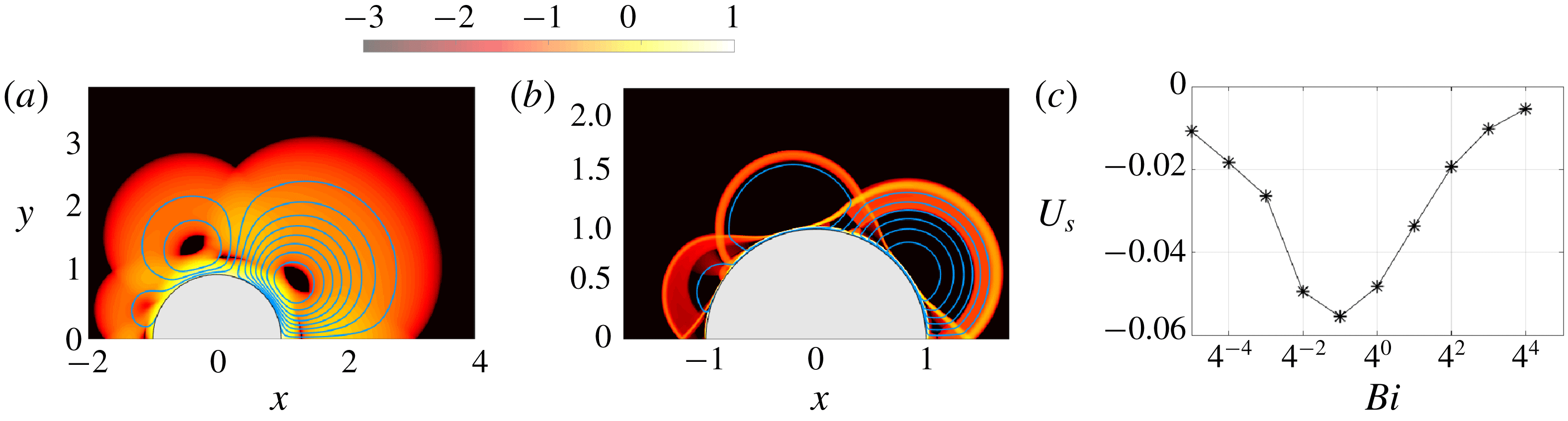
Figure 11. Force-free squirmer solutions for
 $(n,m)=(2,3)$
and
$(n,m)=(2,3)$
and
 $a=1$
showing
$a=1$
showing
 $\log _{10}\dot{\unicode[STIX]{x1D6FE}}$
for (a)
$\log _{10}\dot{\unicode[STIX]{x1D6FE}}$
for (a)
 $Bi=1$
and (b)
$Bi=1$
and (b)
 $Bi=2^{8}$
. (c) The variation of the force-free swimming speed
$Bi=2^{8}$
. (c) The variation of the force-free swimming speed
 $U_{s}$
with
$U_{s}$
with
 $Bi$
.
$Bi$
.
Finally, we report an example exploiting the prescribed normal surface velocity in (2.11), rather than the tangential motions previously discussed. As argued in § 5.2, the simplest example of this model with
 $n=1$
and
$n=1$
and
 $a=0$
is equivalent to the squirmer with the tangential surface velocity
$a=0$
is equivalent to the squirmer with the tangential surface velocity
 $V_{p}=\sin \unicode[STIX]{x1D703}$
, but for the switch in translation speed
$V_{p}=\sin \unicode[STIX]{x1D703}$
, but for the switch in translation speed
 $U_{s}\rightarrow 1-U_{s}$
. Hence, all the results in figures 7 and 9 immediately carry over, although the switch in
$U_{s}\rightarrow 1-U_{s}$
. Hence, all the results in figures 7 and 9 immediately carry over, although the switch in
 $U_{s}$
implies a very different limit for the force-free swimming speed for
$U_{s}$
implies a very different limit for the force-free swimming speed for
 $Bi\gg 1$
. Additional results for
$Bi\gg 1$
. Additional results for
 $m=2$
and varying
$m=2$
and varying
 $a$
are displayed in figure 12. When
$a$
are displayed in figure 12. When
 $a$
is not small, the swimmer is no longer equivalent to a squirmer with tangential surface velocity; larger-scale patterns of plastic deformation develop with both curved sliplines, centred fans and constant-stress triangles. The swimming speed now converges to an
$a$
is not small, the swimmer is no longer equivalent to a squirmer with tangential surface velocity; larger-scale patterns of plastic deformation develop with both curved sliplines, centred fans and constant-stress triangles. The swimming speed now converges to an
 $a$
-dependent constant for
$a$
-dependent constant for
 $Bi\rightarrow \infty$
(the Newtonian limit is again
$Bi\rightarrow \infty$
(the Newtonian limit is again
 $U_{s}\rightarrow \frac{1}{2}$
).
$U_{s}\rightarrow \frac{1}{2}$
).

Figure 12. Force-free squirmer solutions showing
 $\log _{10}\dot{\unicode[STIX]{x1D6FE}}$
for the normal surface velocity condition (2.11) with (a)
$\log _{10}\dot{\unicode[STIX]{x1D6FE}}$
for the normal surface velocity condition (2.11) with (a)
 $a=0.1$
, (b)
$a=0.1$
, (b)
 $0.25$
and (c) 1, at
$0.25$
and (c) 1, at
 $Bi=2^{8}$
. (d) The variation of the swimming speed with
$Bi=2^{8}$
. (d) The variation of the swimming speed with
 $Bi$
.
$Bi$
.
5.4 Boundary-layer theory
5.4.1 Boundary-layer structure
When flow becomes confined to the boundary layer attached to the cylinder, as in figures 9(e,f) and 10(a,b), we rescale the variables to describe that narrow region (cf. appendix A) as follows:
 $$\begin{eqnarray}\displaystyle r=1+Bi^{-1/2}\unicode[STIX]{x1D702},\quad [u,U_{s}]=Bi^{-1/2}[U(\unicode[STIX]{x1D702},\unicode[STIX]{x1D703}),U_{1}],\quad v=V(\unicode[STIX]{x1D702},\unicode[STIX]{x1D703}),\quad p=BiP(\unicode[STIX]{x1D702},\unicode[STIX]{x1D703}). & & \displaystyle \nonumber\\ \displaystyle & & \displaystyle\end{eqnarray}$$
At leading order, local force balance then demands
 $$\begin{eqnarray}\displaystyle P_{\unicode[STIX]{x1D702}}=0\quad \text{and}\quad V_{\unicode[STIX]{x1D702}\unicode[STIX]{x1D702}}+2\text{ sgn }(V_{\unicode[STIX]{x1D702}})=P_{\unicode[STIX]{x1D703}}. & & \displaystyle\end{eqnarray}$$
In terms of the rescaled variables, the boundary conditions in (2.9) become
 $$\begin{eqnarray}\displaystyle V(0,\unicode[STIX]{x1D703})\sim V_{p}(\unicode[STIX]{x1D703})\quad \text{and}\quad U(0,\unicode[STIX]{x1D703})=U_{1}\cos \unicode[STIX]{x1D703}, & & \displaystyle\end{eqnarray}$$
whereas the match to the surrounding plug at the yield surface,
 $\unicode[STIX]{x1D702}=\unicode[STIX]{x1D702}_{b}(\unicode[STIX]{x1D703})$
, demands that
$\unicode[STIX]{x1D702}=\unicode[STIX]{x1D702}_{b}(\unicode[STIX]{x1D703})$
, demands that
 $$\begin{eqnarray}\displaystyle & \displaystyle V(\unicode[STIX]{x1D702}_{b},\unicode[STIX]{x1D703})=V_{\unicode[STIX]{x1D702}}(\unicode[STIX]{x1D702}_{b},\unicode[STIX]{x1D703})=U(\unicode[STIX]{x1D702}_{b},\unicode[STIX]{x1D703})=0. & \displaystyle\end{eqnarray}$$
We therefore find the velocity profile,
 $$\begin{eqnarray}\displaystyle & \displaystyle V=V_{p}(\unicode[STIX]{x1D703})\left(1-\frac{\unicode[STIX]{x1D702}}{\unicode[STIX]{x1D702}_{b}}\right)^{2}, & \displaystyle\end{eqnarray}$$
with
 $$\begin{eqnarray}\displaystyle & \displaystyle P_{\unicode[STIX]{x1D703}}=2\left(\frac{|V_{p}|}{\unicode[STIX]{x1D702}_{b}^{2}}-1\right)\;\text{sgn}(V_{p}). & \displaystyle\end{eqnarray}$$
The integral of the leading-order continuity equation,
 $V_{\unicode[STIX]{x1D703}}+U_{\unicode[STIX]{x1D702}}\sim 0$
across the boundary layer now furnishes
$V_{\unicode[STIX]{x1D703}}+U_{\unicode[STIX]{x1D702}}\sim 0$
across the boundary layer now furnishes
 $$\begin{eqnarray}\displaystyle & \displaystyle \frac{\unicode[STIX]{x2202}}{\unicode[STIX]{x2202}\unicode[STIX]{x1D703}}\left[\frac{\unicode[STIX]{x1D702}_{b}V_{p}(\unicode[STIX]{x1D703})}{3}\right]-U_{1}\cos \unicode[STIX]{x1D703}=0. & \displaystyle\end{eqnarray}$$
Focussing on surface motions that are up–down antisymmetric with
 $V_{p}(0)=V_{p}(\unicode[STIX]{x03C0})=0$
, we now find the boundary-layer profile,
$V_{p}(0)=V_{p}(\unicode[STIX]{x03C0})=0$
, we now find the boundary-layer profile,
 $$\begin{eqnarray}\displaystyle & \displaystyle \unicode[STIX]{x1D702}_{b}(\unicode[STIX]{x1D703})=\frac{3U_{1}\sin \unicode[STIX]{x1D703}}{V_{p}(\unicode[STIX]{x1D703})}. & \displaystyle\end{eqnarray}$$
This thickness is only positive when the angular surface motion
 $V_{p}(\unicode[STIX]{x1D703})$
is directed opposite to the sense of translation,
$V_{p}(\unicode[STIX]{x1D703})$
is directed opposite to the sense of translation,
 $\text{sgn}(U_{s})$
. Otherwise, the balances implied by the scalings in (5.3) are not consistent, which we interpret to signify that the flow cannot be confined to the surface boundary layer. Indeed, the numerical solutions in § 5.3 display larger-scale flow patterns at large
$\text{sgn}(U_{s})$
. Otherwise, the balances implied by the scalings in (5.3) are not consistent, which we interpret to signify that the flow cannot be confined to the surface boundary layer. Indeed, the numerical solutions in § 5.3 display larger-scale flow patterns at large
 $Bi$
whenever
$Bi$
whenever
 $U_{s}/V_{p}<0$
.
$U_{s}/V_{p}<0$
.
Figure 13 compares the predictions of (5.10) with some of the measured yield surfaces of the numerical solution with confined flow patterns. In the simple case with
 $V_{p}(\unicode[STIX]{x1D703})=\sin \unicode[STIX]{x1D703}$
(figure 13
a), the boundary layer has the constant width,
$V_{p}(\unicode[STIX]{x1D703})=\sin \unicode[STIX]{x1D703}$
(figure 13
a), the boundary layer has the constant width,
 $\unicode[STIX]{x1D702}_{b}=(r_{p}-1)Bi^{1/2}=\sqrt{\unicode[STIX]{x03C0}/2}$
, where
$\unicode[STIX]{x1D702}_{b}=(r_{p}-1)Bi^{1/2}=\sqrt{\unicode[STIX]{x03C0}/2}$
, where
 $r_{p}$
is the radius of the yield surface. The yield surfaces of the computations are indeed relatively flat and compare well with the prediction, except close to the front and back of the cylinder where the boundary-layer thickness sharply declines over further ‘corner regions’. For squirmers with
$r_{p}$
is the radius of the yield surface. The yield surfaces of the computations are indeed relatively flat and compare well with the prediction, except close to the front and back of the cylinder where the boundary-layer thickness sharply declines over further ‘corner regions’. For squirmers with
 $V_{p}=\sin \unicode[STIX]{x1D703}+a\sin m\unicode[STIX]{x1D703}$
, the boundary-layer thickness varies with position; again the predictions match well with numerical results except for the adjustments at the front and back (figure 13(b,c)).
$V_{p}=\sin \unicode[STIX]{x1D703}+a\sin m\unicode[STIX]{x1D703}$
, the boundary-layer thickness varies with position; again the predictions match well with numerical results except for the adjustments at the front and back (figure 13(b,c)).

Figure 13. Boundary-layer thicknesses of squirmers for (a)
 $(n,a)=(1,0)$
, (b)
$(n,a)=(1,0)$
, (b)
 $(n,m,a)=(1,2,0.25)$
and (c)
$(n,m,a)=(1,2,0.25)$
and (c)
 $(n,m,a)=(1,3,0.25)$
, with
$(n,m,a)=(1,3,0.25)$
, with
 $Bi=2^{6}$
(black),
$Bi=2^{6}$
(black),
 $Bi=2^{8}$
(blue),
$Bi=2^{8}$
(blue),
 $Bi=2^{10}$
(red) and
$Bi=2^{10}$
(red) and
 $Bi=2^{12}$
(green). The prediction from (5.10) is shown by dashed lines.
$Bi=2^{12}$
(green). The prediction from (5.10) is shown by dashed lines.
For
 $V_{p}U_{1}<0$
, the emergence of plastic deformation outside the boundary layer (with
$V_{p}U_{1}<0$
, the emergence of plastic deformation outside the boundary layer (with
 $(u,v)\sim O(Bi^{-1/2})$
) modifies the final boundary condition in (5.5), and therefore the flux balance in (5.9). The resulting flow into or out of the boundary layer then maintains a boundary layer of finite thickness. Importantly, however, the scalings of the boundary layer in (5.3), do not change although one must now complete the solution by matching to the adjacent region of perfectly plastic deformation (which we avoid here).
$(u,v)\sim O(Bi^{-1/2})$
) modifies the final boundary condition in (5.5), and therefore the flux balance in (5.9). The resulting flow into or out of the boundary layer then maintains a boundary layer of finite thickness. Importantly, however, the scalings of the boundary layer in (5.3), do not change although one must now complete the solution by matching to the adjacent region of perfectly plastic deformation (which we avoid here).
5.4.2 Drag force and swimming speed
Given the surface pressure
 $BiP$
and tangential shear stress
$BiP$
and tangential shear stress
 $Bi\;\text{sgn}(V_{\unicode[STIX]{x1D702}})=-Bi\;\text{sgn}(V_{p})$
, the net horizontal force on the swimmer is given by
$Bi\;\text{sgn}(V_{\unicode[STIX]{x1D702}})=-Bi\;\text{sgn}(V_{p})$
, the net horizontal force on the swimmer is given by
 $$\begin{eqnarray}F_{x}=-Bi\int _{-\unicode[STIX]{x03C0}}^{\unicode[STIX]{x03C0}}[P\cos \unicode[STIX]{x1D703}-\text{sgn}(V_{p})\sin \unicode[STIX]{x1D703}]\,\text{d}\unicode[STIX]{x1D703}=2Bi\int _{0}^{\unicode[STIX]{x03C0}}\left(\frac{2|V_{p}|^{3}}{9U_{1}^{2}\sin \unicode[STIX]{x1D703}}-\sin \unicode[STIX]{x1D703}\right)\text{sgn}(V_{p})\,\text{d}\unicode[STIX]{x1D703}.\end{eqnarray}$$
The drag therefore vanishes for
 $$\begin{eqnarray}\displaystyle & \displaystyle U_{s}^{ff}=\frac{Bi^{-1/2}}{3}\sqrt{2\int _{0}^{\unicode[STIX]{x03C0}}\frac{V_{p}(\unicode[STIX]{x1D703})^{3}}{\sin \unicode[STIX]{x1D703}}\,\text{d}\unicode[STIX]{x1D703}}\left[\int _{0}^{\unicode[STIX]{x03C0}}\sin \unicode[STIX]{x1D703}\;\text{sgn}(V_{p})\,\text{d}\unicode[STIX]{x1D703}\right]^{-1/2}, & \displaystyle\end{eqnarray}$$
furnishing an asymptotic prediction of the locomotion speed of the force-free swimmer.
The drag from (5.11) also increases with decreasing translation speed
 $U_{s}$
, diverging for
$U_{s}$
, diverging for
 $U_{s}\rightarrow 0$
, and must therefore exceed that associated with the Randolph and Houlsby slipline solution below some threshold in
$U_{s}\rightarrow 0$
, and must therefore exceed that associated with the Randolph and Houlsby slipline solution below some threshold in
 $U_{s}$
. We interpret the crossover to correspond to the switch from the confined flow pattern to larger-scale plastic deformation. The deconfinement of the flow must therefore occur for
$U_{s}$
. We interpret the crossover to correspond to the switch from the confined flow pattern to larger-scale plastic deformation. The deconfinement of the flow must therefore occur for
 $$\begin{eqnarray}\displaystyle U_{s}=U_{s}^{ff}\left\{1+2(\unicode[STIX]{x03C0}+2\sqrt{2})\left[\int _{0}^{\unicode[STIX]{x03C0}}\sin \unicode[STIX]{x1D703}\;\text{sgn}(V_{p})\,\text{d}\unicode[STIX]{x1D703}\right]^{-1}\right\}^{-1/2}. & & \displaystyle\end{eqnarray}$$
For the simplest case with
 $V_{p}=\sin \unicode[STIX]{x1D703}$
(
$V_{p}=\sin \unicode[STIX]{x1D703}$
(
 $n=1$
,
$n=1$
,
 $a=0$
), the drag coefficient implied by (5.11) is
$a=0$
), the drag coefficient implied by (5.11) is
 $$\begin{eqnarray}\displaystyle & \displaystyle C_{d}=-\frac{F_{x}}{2Bi}=2-\frac{\unicode[STIX]{x03C0}}{9U_{1}^{2}}, & \displaystyle\end{eqnarray}$$
which is compared to the numerical results in figure 7(g); the switch in flow pattern for (5.13) also matches satisfyingly with the abrupt drop in the magnitude of
 $C_{d}$
in the numerical solutions. The corresponding force-free swimmer has
$C_{d}$
in the numerical solutions. The corresponding force-free swimmer has
 $U_{s}^{ff}=\sqrt{\unicode[STIX]{x03C0}/18}Bi^{-1/2}$
, which again compares well with the numerical results (figure 7
g).
$U_{s}^{ff}=\sqrt{\unicode[STIX]{x03C0}/18}Bi^{-1/2}$
, which again compares well with the numerical results (figure 7
g).
For squirmers with
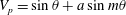 $V_{p}=\sin \unicode[STIX]{x1D703}+a\sin m\unicode[STIX]{x1D703}$
, the swimming speed is
$V_{p}=\sin \unicode[STIX]{x1D703}+a\sin m\unicode[STIX]{x1D703}$
, the swimming speed is
 $$\begin{eqnarray}\displaystyle U_{s}^{ff}=\left\{\begin{array}{@{}ll@{}}{\textstyle \frac{1}{3}}Bi^{-1/2}\sqrt{{\textstyle \frac{1}{2}}\unicode[STIX]{x03C0}(1+3a^{2})}, & m\text{ even,}\\[12.0pt] {\textstyle \frac{1}{3}}Bi^{-1/2}\sqrt{{\textstyle \frac{1}{2}}\unicode[STIX]{x03C0}(1+3a^{2}+a^{3})}, & m\text{ odd,}\end{array}\right. & & \displaystyle\end{eqnarray}$$
provided the boundary-layer thickness remains finite everywhere, which demands that
 $a<m^{-1}$
for
$a<m^{-1}$
for
 $m$
even and
$m$
even and
 $a\lesssim \sin (3\unicode[STIX]{x03C0}/2m)$
for
$a\lesssim \sin (3\unicode[STIX]{x03C0}/2m)$
for
 $m$
odd. Figures 9(j) and 10(g) include the predictions in (5.15).
$m$
odd. Figures 9(j) and 10(g) include the predictions in (5.15).
Note that the prediction for the swimming speed in (5.12) relies on the solutions in (5.8) and (5.10), which fail when flow is no longer confined to the boundary layer. Nevertheless, because the scalings of the problem do not change in that situation, the swimming speed still scales with
 $Bi^{-1/2}$
, as seen in the numerical computations (e.g. figure 9
i). The match to the surrounding plastic deformation, however, determines the coefficient
$Bi^{-1/2}$
, as seen in the numerical computations (e.g. figure 9
i). The match to the surrounding plastic deformation, however, determines the coefficient
 $U_{1}$
.
$U_{1}$
.
6 Conclusions
In this paper, we have investigated viscoplastic flows around cylinders, with an emphasis on the limit of large yield stress. For a translating cylinder with a no-slip surface, we compared analytical plasticity solutions based on slipline theory with viscoplastic computations. Significant differences between the two arise due to the presence of rigidly rotating plugs above and below the cylinder in the computations, which are not present in the slipline solutions. These plugs ride on top of the viscous boundary layer that shrouds the cylinder, leading one to wonder whether they interfere with the plastic limit of the viscoplastic model. By performing a suite of careful computations and developing a boundary-layer theory, we showed that such features do actually disappear in the plastic limit (
 $Bi\rightarrow \infty$
), implying that viscoplasticity does converge to ideal plasticity.
$Bi\rightarrow \infty$
), implying that viscoplasticity does converge to ideal plasticity.
We then modified the boundary condition on the translating cylinder to allow for partial slip over its surface. This situation corresponds to partially rough cylinders in ideal plasticity, for which the slipline solution has not previously been identified, with an original construction proposed by Randolph & Houlsby (Reference Randolph and Houlsby1984) having been shown to be inconsistent for partial slip (Murff et al. Reference Murff, Wagner and Randolph1989; Martin & Randolph Reference Martin and Randolph2006). Instead, we found our computations matched with an alternative slipline pattern proposed by Martin & Randolph (Reference Martin and Randolph2006) as an upper bound solution based on its velocity field. This alternative pattern contains genuine rigid plugs rotating above and below the cylinder, attached to, and sliding over, the surface. Delving further into Martin and Randolph’s slipline construction, we found that the stress solution suggests a lower bound that matches the upper bound provided the rotating plugs are free of any net torque. This implies that the slipline field actually provides the true plastic solution. However, the slipline theory is incomplete in this example because no stress field is provided for the plugs that matches the partially rough surface conditions and is consistent with the yield condition. Nevertheless, the computations do explicitly construct an acceptable stress field for the plugs, providing numerical evidence for the conclusion that Martin and Randolph’s slipline pattern is the true plastic solution.
The slipline patterns of the translating cylinders provide a set of tools to understand viscoplastic flow around cylinders with a variety of other surface conditions. In the third thread of this study, we applied this idea to models of cylindrical ‘squirmers’ swimming in yield-stress fluid. The slipline patterns do indeed characterize many of the flow structures seen around such model micro-organisms when we approach the plastic limit. However, we also found that flow can become consumed into the viscous boundary layers against the cylinder surfaces, allowing us to analytically construct the swimming states. We provided the viscoplastic analogues of squirming ‘pushers’ and ‘pullers’, for which the driving surface velocity is concentrated either to the back or front of the cylinder. While these squirmers have identical swimming speeds, as in the Newtonian limit, we also identified driving surface velocity patterns for which this symmetry is not preserved if the fluid has a yield stress. We also provided examples of swimming patterns that would be immobile in the Newtonian limit, but may swim when there is yield stress because of the nonlinearity of the fluid rheology.
For squirmers driven by a prescribed tangential surface velocity in Newtonian fluid, without considering the specific details of the surface velocity pattern, the swimming speed
 ${\mathcal{U}}_{s}$
scales with the characteristic speed of the driving surface velocity
${\mathcal{U}}_{s}$
scales with the characteristic speed of the driving surface velocity
 ${\mathcal{U}}$
and the power input per unit swimming speed and cylinder length is
${\mathcal{U}}$
and the power input per unit swimming speed and cylinder length is
 ${\mathcal{P}}\sim \unicode[STIX]{x1D707}{\mathcal{U}}$
. In the opposite, plastic limit, the swimming speed and power turn out to scale as
${\mathcal{P}}\sim \unicode[STIX]{x1D707}{\mathcal{U}}$
. In the opposite, plastic limit, the swimming speed and power turn out to scale as
 $$\begin{eqnarray}\displaystyle {\mathcal{U}}_{s}\sim {\mathcal{U}}^{3/2}\sqrt{\frac{\unicode[STIX]{x1D707}}{\unicode[STIX]{x1D70F}_{Y}{\mathcal{R}}}}\quad \text{and}\quad {\mathcal{P}}\sim \frac{{\mathcal{R}}{\mathcal{U}}\unicode[STIX]{x1D70F}_{r\unicode[STIX]{x1D703}}}{{\mathcal{U}}_{s}}\sim \frac{(\unicode[STIX]{x1D70F}_{Y}{\mathcal{R}})^{3/2}}{(\unicode[STIX]{x1D707}{\mathcal{U}})^{1/2}}, & & \displaystyle\end{eqnarray}$$
if
 ${\mathcal{R}}$
is the cylinder radius and
${\mathcal{R}}$
is the cylinder radius and
 $\unicode[STIX]{x1D707}$
and
$\unicode[STIX]{x1D707}$
and
 $\unicode[STIX]{x1D70F}_{Y}$
are the fluid (plastic) viscosity and yield stress. The decaying dependence on yield stress and presence of the viscosity is symptomatic of the viscous boundary layers against the cylinder surface which activate locomotion (the
$\unicode[STIX]{x1D70F}_{Y}$
are the fluid (plastic) viscosity and yield stress. The decaying dependence on yield stress and presence of the viscosity is symptomatic of the viscous boundary layers against the cylinder surface which activate locomotion (the
 $Bi^{-1/2}$
layers in § 5). Note that the effective viscosity of the medium in the plastic limit is
$Bi^{-1/2}$
layers in § 5). Note that the effective viscosity of the medium in the plastic limit is
 $\unicode[STIX]{x1D707}_{eff}\sim \unicode[STIX]{x1D70F}_{Y}{\mathcal{R}}/{\mathcal{U}}\gg \unicode[STIX]{x1D707}$
(being given by the relatively large yield stress). Therefore, the scaling of the swimming speed is
$\unicode[STIX]{x1D707}_{eff}\sim \unicode[STIX]{x1D70F}_{Y}{\mathcal{R}}/{\mathcal{U}}\gg \unicode[STIX]{x1D707}$
(being given by the relatively large yield stress). Therefore, the scaling of the swimming speed is
 ${\mathcal{U}}_{s}\sim {\mathcal{U}}\sqrt{\unicode[STIX]{x1D707}/\unicode[STIX]{x1D707}_{eff}}$
, which implies that the swimmer moves much slower in the viscoplastic medium than in a Newtonian fluid with the same effective viscosity
${\mathcal{U}}_{s}\sim {\mathcal{U}}\sqrt{\unicode[STIX]{x1D707}/\unicode[STIX]{x1D707}_{eff}}$
, which implies that the swimmer moves much slower in the viscoplastic medium than in a Newtonian fluid with the same effective viscosity
 $\unicode[STIX]{x1D707}_{eff}$
, for a given surface velocity pattern. Moreover, the input power per unit length and swimming speed is
$\unicode[STIX]{x1D707}_{eff}$
, for a given surface velocity pattern. Moreover, the input power per unit length and swimming speed is
 ${\mathcal{P}}\sim \unicode[STIX]{x1D707}_{eff}\,{\mathcal{U}}\sqrt{\unicode[STIX]{x1D707}_{eff}/\unicode[STIX]{x1D707}}$
, rather larger than the Newtonian equivalent (
${\mathcal{P}}\sim \unicode[STIX]{x1D707}_{eff}\,{\mathcal{U}}\sqrt{\unicode[STIX]{x1D707}_{eff}/\unicode[STIX]{x1D707}}$
, rather larger than the Newtonian equivalent (
 $\unicode[STIX]{x1D707}_{eff}\,{\mathcal{U}}$
).
$\unicode[STIX]{x1D707}_{eff}\,{\mathcal{U}}$
).
Thus, swimming by tangential squirming motions in a nearly plastic medium is relatively inefficient, primarily as a result of the lubricating effect of the viscous boundary layers against the cylinder’s surface. The situation is quite different if swimming is driven by normal surface motions, for which we have given a briefer discussion. The swimming speed in the plastic limit then remains of order
 ${\mathcal{U}}$
, as in the Newtonian limit, and the corresponding power input per unit swimming speed and length is given by
${\mathcal{U}}$
, as in the Newtonian limit, and the corresponding power input per unit swimming speed and length is given by
 ${\mathcal{P}}\sim \unicode[STIX]{x1D70F}_{Y}{\mathcal{R}}\sim \unicode[STIX]{x1D707}_{eff}\,{\mathcal{U}}$
. Now the swimming speed and power input are comparable to those for motion through Newtonian fluid with viscosity
${\mathcal{P}}\sim \unicode[STIX]{x1D70F}_{Y}{\mathcal{R}}\sim \unicode[STIX]{x1D707}_{eff}\,{\mathcal{U}}$
. Now the swimming speed and power input are comparable to those for motion through Newtonian fluid with viscosity
 $\unicode[STIX]{x1D707}_{eff}$
(a situation shared by the viscoplastic version of Taylor’s swimming sheet, considered by Hewitt & Balmforth (Reference Hewitt and Balmforth2017)).
$\unicode[STIX]{x1D707}_{eff}$
(a situation shared by the viscoplastic version of Taylor’s swimming sheet, considered by Hewitt & Balmforth (Reference Hewitt and Balmforth2017)).
Another key feature of the swimming dynamics is that the yield stress always limits flow to within a yield surface that lies at a finite distance from the squirmer. This has important implications for the induced transport of nutrients or other tracers and the hydrodynamic interactions and collective dynamics of multiple swimmers (Lauga & Powers Reference Lauga and Powers2009; Pedley Reference Pedley2016). Finally, we add a cautionary note that our modelling of swimming micro-organisms as cylinders with prescribed surface motions is somewhat restrictive, limiting the quantitative application of our results. In particular, we neglect all effects of viscoplasticity on the imposed surface velocity pattern, and a real concern is that the cilia responsible for driving these motions may themselves clog up under the action of the yield stress. However, the qualitative results of our work constitute a first step towards understanding the effect of a yield stress on true squirming swimmers.
Acknowledgements
This work was largely conducted at the Geophysical Fluid Dynamics Summer Study program, Woods Hole Oceanographic Institution, which is supported by the National Science Foundation. We thank S. Mandre, in particular, for helpful conversations.
Appendix A. Viscoplastic boundary layers for a no-slip cylinder
In this appendix, we outline a boundary-layer theory for a translating cylinder with a no-slip surface. To set the scene, figure 14 shows a magnification of the boundary-layer structure below the upper rotating plug.

Figure 14. A magnification of the region underneath the upper rotating plug for a no-slip cylinder with
 $Bi=2^{12}$
. The colour shading shows
$Bi=2^{12}$
. The colour shading shows
 $\log _{10}\dot{\unicode[STIX]{x1D6FE}}$
, and the blue lines are streamlines. The black lines display the
$\log _{10}\dot{\unicode[STIX]{x1D6FE}}$
, and the blue lines are streamlines. The black lines display the
 $\unicode[STIX]{x1D6FC}$
-lines of the slipline solution, selected to coincide with the streamlines at
$\unicode[STIX]{x1D6FC}$
-lines of the slipline solution, selected to coincide with the streamlines at
 $\unicode[STIX]{x1D703}=\frac{1}{2}\unicode[STIX]{x03C0}$
.
$\unicode[STIX]{x1D703}=\frac{1}{2}\unicode[STIX]{x03C0}$
.
A.1 Beyond the rotating plug
Outside the region directly underneath the plug, the main balance of forces expected for the boundary layer against the surface of the cylinder is given by
 $$\begin{eqnarray}\displaystyle p_{r}\sim 0\quad \text{and}\quad p_{\unicode[STIX]{x1D703}}\sim (r^{2}\unicode[STIX]{x1D70F}_{r\unicode[STIX]{x1D703}})_{r},\quad \text{where }\unicode[STIX]{x1D70F}_{r\unicode[STIX]{x1D703}}\sim v_{r}+Bi\,\text{sgn}(v_{r}) & & \displaystyle\end{eqnarray}$$
(see Balmforth et al. (Reference Balmforth, Craster, Hewitt, Hormozi and Maleki2017)). The solution must match to the nearly perfectly plastic flow outside the boundary layer, where the pressure is given by (3.1), the velocity is directed along the
 $\unicode[STIX]{x1D6FC}$
-lines and the shear rates are much weaker. The latter two conditions translate to
$\unicode[STIX]{x1D6FC}$
-lines and the shear rates are much weaker. The latter two conditions translate to
 $v(r_{b})\sim 0$
and
$v(r_{b})\sim 0$
and
 $v_{r}(r_{b})\sim 0$
, where
$v_{r}(r_{b})\sim 0$
, where
 $r_{b}$
is the edge of the boundary layer. Hence, after incorporating the no-slip condition
$r_{b}$
is the edge of the boundary layer. Hence, after incorporating the no-slip condition
 $v(1)=\sin \unicode[STIX]{x1D703}$
, we find
$v(1)=\sin \unicode[STIX]{x1D703}$
, we find
 $$\begin{eqnarray}\displaystyle v=-2Bi(r_{b}-r)^{2}\text{ sgn}(\sin \unicode[STIX]{x1D703}),\quad r_{b}=1+Bi^{-1/2}\sqrt{{\textstyle \frac{1}{2}}|\text{sin}\unicode[STIX]{x1D703}|}, & & \displaystyle\end{eqnarray}$$
indicating that the thickness of the boundary layer is
 $O(Bi^{-1/2})$
. Such parabolic velocity profiles have been noted previously by Tokpavi et al. (Reference Tokpavi, Magnin and Jay2008).
$O(Bi^{-1/2})$
. Such parabolic velocity profiles have been noted previously by Tokpavi et al. (Reference Tokpavi, Magnin and Jay2008).
A.2 Underneath the rotating plug
Directly underneath the rotating plug where the pressure jump is smoothed, the angular scale becomes smaller and we rescale the variables to reflect this whilst maintaining the main balances demanded by force balance and the continuity equation,
 $$\begin{eqnarray}\displaystyle (r,\unicode[STIX]{x1D703})=\left(1+Bi^{-a}\unicode[STIX]{x1D709},{\textstyle \frac{1}{2}}\unicode[STIX]{x03C0}-Bi^{-b}\unicode[STIX]{x1D6E9}\right),\quad [u,v]\sim [Bi^{b-a}U(\unicode[STIX]{x1D709},\unicode[STIX]{x1D6E9}),V(\unicode[STIX]{x1D709},\unicode[STIX]{x1D6E9})],\quad & & \displaystyle\end{eqnarray}$$
 $$\begin{eqnarray}\displaystyle p\sim BiP(\unicode[STIX]{x1D709},\unicode[STIX]{x1D6E9})\quad \text{and}\quad \unicode[STIX]{x1D70F}_{\unicode[STIX]{x1D709}\unicode[STIX]{x1D6E9}}\sim Bi^{a}V_{\unicode[STIX]{x1D709}}-Bi, & & \displaystyle\end{eqnarray}$$
where
 $\unicode[STIX]{x1D702}$
and
$\unicode[STIX]{x1D702}$
and
 $\unicode[STIX]{x1D6E9}$
are
$\unicode[STIX]{x1D6E9}$
are
 $O(1)$
, and the exponents
$O(1)$
, and the exponents
 $a>\frac{1}{2}$
and
$a>\frac{1}{2}$
and
 $b>0$
satisfy
$b>0$
satisfy
 $2a=1+b$
. The force balance in (A 1) then becomes
$2a=1+b$
. The force balance in (A 1) then becomes
 $$\begin{eqnarray}\displaystyle P_{\unicode[STIX]{x1D709}}\sim 0\quad \text{and}\quad P_{\unicode[STIX]{x1D6E9}}\sim V_{\unicode[STIX]{x1D709}\unicode[STIX]{x1D709}}. & & \displaystyle\end{eqnarray}$$
The no-slip condition is now
 $V(0)\sim 1$
, whereas matching again demands that
$V(0)\sim 1$
, whereas matching again demands that
 $(V,V_{\unicode[STIX]{x1D709}})\rightarrow 0$
at the edge of the boundary layer
$(V,V_{\unicode[STIX]{x1D709}})\rightarrow 0$
at the edge of the boundary layer
 $\unicode[STIX]{x1D709}=\unicode[STIX]{x1D6EF}(\unicode[STIX]{x1D6E9})$
. Hence,
$\unicode[STIX]{x1D709}=\unicode[STIX]{x1D6EF}(\unicode[STIX]{x1D6E9})$
. Hence,
 $$\begin{eqnarray}\displaystyle & \displaystyle V\sim -\left(1-\frac{\unicode[STIX]{x1D709}}{\unicode[STIX]{x1D6EF}}\right)^{2}\text{sgn}(y)\quad \text{and}\quad P_{\unicode[STIX]{x1D6E9}}=-\frac{2}{\unicode[STIX]{x1D6EF}^{2}}\text{sgn}(y). & \displaystyle\end{eqnarray}$$
At this stage, unlike in (A 2), we cannot match
 $P$
to the pressure of the slipline solution to determine the boundary-layer profile
$P$
to the pressure of the slipline solution to determine the boundary-layer profile
 $\unicode[STIX]{x1D6EF}(\unicode[STIX]{x1D6E9})$
because of the intervention of the rotating plug. Instead, we proceed by dividing up the boundary layer into the part surrounding
$\unicode[STIX]{x1D6EF}(\unicode[STIX]{x1D6E9})$
because of the intervention of the rotating plug. Instead, we proceed by dividing up the boundary layer into the part surrounding
 $\unicode[STIX]{x1D703}=\frac{1}{2}\unicode[STIX]{x03C0}$
that is directly attached to the rotating plug, and the part beyond where the boundary layer detaches from the plug and another nearly perfectly plastic flow separates the two. For the first part, the rigid rotation of the plug implies a velocity field of
$\unicode[STIX]{x1D703}=\frac{1}{2}\unicode[STIX]{x03C0}$
that is directly attached to the rotating plug, and the part beyond where the boundary layer detaches from the plug and another nearly perfectly plastic flow separates the two. For the first part, the rigid rotation of the plug implies a velocity field of
 $(u,v)=\unicode[STIX]{x1D714}(\cos \unicode[STIX]{x1D703},r-\sin \unicode[STIX]{x1D703})$
, where the rotation rate is observed from the numerical computations to be
$(u,v)=\unicode[STIX]{x1D714}(\cos \unicode[STIX]{x1D703},r-\sin \unicode[STIX]{x1D703})$
, where the rotation rate is observed from the numerical computations to be
 $\unicode[STIX]{x1D714}\sim 1-Bi^{-c}\unicode[STIX]{x1D6FA}$
, with
$\unicode[STIX]{x1D714}\sim 1-Bi^{-c}\unicode[STIX]{x1D6FA}$
, with
 $\unicode[STIX]{x1D6FA}>0$
; see figure 3(a). If we now integrate the leading-order continuity equation,
$\unicode[STIX]{x1D6FA}>0$
; see figure 3(a). If we now integrate the leading-order continuity equation,
 $U_{\unicode[STIX]{x1D6EF}}-V_{\unicode[STIX]{x1D6E9}}\sim 0$
, over the boundary layer from
$U_{\unicode[STIX]{x1D6EF}}-V_{\unicode[STIX]{x1D6E9}}\sim 0$
, over the boundary layer from
 $\unicode[STIX]{x1D709}=0$
to
$\unicode[STIX]{x1D709}=0$
to
 $\unicode[STIX]{x1D709}=\unicode[STIX]{x1D6EF}$
, we find
$\unicode[STIX]{x1D709}=\unicode[STIX]{x1D6EF}$
, we find
 $$\begin{eqnarray}\displaystyle & \displaystyle \left[\int _{0}^{\unicode[STIX]{x1D6EF}}\left(1-\frac{\unicode[STIX]{x1D709}}{\unicode[STIX]{x1D6EF}}\right)^{2}\,\text{d}\unicode[STIX]{x1D709}\right]_{\unicode[STIX]{x1D6E9}}=\frac{1}{3}\unicode[STIX]{x1D6EF}_{\unicode[STIX]{x1D6E9}}=U(0,\unicode[STIX]{x1D6E9})-U(\unicode[STIX]{x1D6EF},\unicode[STIX]{x1D6E9}) & \displaystyle\end{eqnarray}$$
 $$\begin{eqnarray}\displaystyle & \displaystyle \equiv Bi^{a-b}(1-\unicode[STIX]{x1D714})\cos \unicode[STIX]{x1D703}\sim Bi^{a-2b-c}\unicode[STIX]{x1D6FA}\unicode[STIX]{x1D6E9}. & \displaystyle\end{eqnarray}$$
Hence
 $2b+c=a$
and
$2b+c=a$
and
 $$\begin{eqnarray}\displaystyle & \displaystyle \unicode[STIX]{x1D6EF}(\unicode[STIX]{x1D6E9})=\unicode[STIX]{x1D6EF}(0)+{\textstyle \frac{3}{2}}\unicode[STIX]{x1D6FA}\unicode[STIX]{x1D6E9}^{2}, & \displaystyle\end{eqnarray}$$
which thickens away from the centre of the fan at
 $A$
, unlike the profile in (A 2).
$A$
, unlike the profile in (A 2).
For the part of the smoothing region where the plug has detached from the boundary layer, there is an intervening window of purely plastic deformation in which the velocity field is adjusted away from rigid rotation. Because this window is relatively small, the
 $\unicode[STIX]{x1D6FC}$
-lines remain close to the involutes of the perfectly plastic slipline solution, which begin at the angular location
$\unicode[STIX]{x1D6FC}$
-lines remain close to the involutes of the perfectly plastic slipline solution, which begin at the angular location
 $\unicode[STIX]{x1D703}=\unicode[STIX]{x03C0}/2-Bi^{-b}\unicode[STIX]{x1D6E9}$
and reach the base of the plug for
$\unicode[STIX]{x1D703}=\unicode[STIX]{x03C0}/2-Bi^{-b}\unicode[STIX]{x1D6E9}$
and reach the base of the plug for
 $y\sim 1$
and
$y\sim 1$
and
 $x=Bi^{-b}\unicode[STIX]{x1D6E9}$
. This proximity indicates that
$x=Bi^{-b}\unicode[STIX]{x1D6E9}$
. This proximity indicates that
 $u\sim Bi^{-b}\unicode[STIX]{x1D714}\unicode[STIX]{x1D6E9}-Bi^{b-a}\unicode[STIX]{x1D71B}(\unicode[STIX]{x1D6E9})$
at the edge of the boundary layer, where the correction
$u\sim Bi^{-b}\unicode[STIX]{x1D714}\unicode[STIX]{x1D6E9}-Bi^{b-a}\unicode[STIX]{x1D71B}(\unicode[STIX]{x1D6E9})$
at the edge of the boundary layer, where the correction
 $Bi^{b-a}\unicode[STIX]{x1D71B}(\unicode[STIX]{x1D6E9})$
represents the velocity adjustment incurred by the modification to the slipline. Thence,
$Bi^{b-a}\unicode[STIX]{x1D71B}(\unicode[STIX]{x1D6E9})$
represents the velocity adjustment incurred by the modification to the slipline. Thence,
 $$\begin{eqnarray}\displaystyle {\textstyle \frac{1}{3}}\unicode[STIX]{x1D6EF}_{\unicode[STIX]{x1D6E9}}\sim U(0,\unicode[STIX]{x1D6E9})-U(\unicode[STIX]{x1D6EF},\unicode[STIX]{x1D703})\sim \unicode[STIX]{x1D71B}(\unicode[STIX]{x1D6E9})+\unicode[STIX]{x1D6FA}\unicode[STIX]{x1D6E9}-{\textstyle \frac{1}{6}}Bi^{a-4b}\unicode[STIX]{x1D6E9}^{3}, & & \displaystyle\end{eqnarray}$$
which indicates that
 $a=4b$
, since all the terms must come in at the same order of
$a=4b$
, since all the terms must come in at the same order of
 $Bi$
because the boundary layer remains continuous across the point of detachment. The combined results for the scalings now indicate that
$Bi$
because the boundary layer remains continuous across the point of detachment. The combined results for the scalings now indicate that
 $$\begin{eqnarray}\displaystyle a={\textstyle \frac{4}{7}},\quad b={\textstyle \frac{1}{7}}\quad \text{and}\quad c={\textstyle \frac{2}{7}}; & & \displaystyle\end{eqnarray}$$
i.e. the boundary-layer thickness scales as
 $Bi^{-4/7}$
underneath the rotating plug, the angular width of the smoothing region scales as
$Bi^{-4/7}$
underneath the rotating plug, the angular width of the smoothing region scales as
 $Bi^{-1/7}$
and the rotation rate of the plug approaches 1 with a scaling of
$Bi^{-1/7}$
and the rotation rate of the plug approaches 1 with a scaling of
 $Bi^{-2/7}$
(figure 3
b).
$Bi^{-2/7}$
(figure 3
b).
Beyond the detachment of the plug, (A 10) implies that the boundary layer profile becomes modified to
 $$\begin{eqnarray}\displaystyle \unicode[STIX]{x1D6EF}(\unicode[STIX]{x1D6E9})\sim \unicode[STIX]{x1D6EF}_{\ast }+\int _{\unicode[STIX]{x1D6E9}_{\ast }}^{\unicode[STIX]{x1D6E9}}\unicode[STIX]{x1D71B}\,\text{d}\unicode[STIX]{x1D6E9}-{\textstyle \frac{1}{8}}(\unicode[STIX]{x1D6E9}^{4}-\unicode[STIX]{x1D6E9}_{\ast }^{4})+{\textstyle \frac{3}{2}}\unicode[STIX]{x1D6FA}\unicode[STIX]{x1D6E9}^{2}, & & \displaystyle\end{eqnarray}$$
where
 $\unicode[STIX]{x1D6E9}_{\ast }$
denotes the angle of detachment and the corresponding boundary-layer thickness is
$\unicode[STIX]{x1D6E9}_{\ast }$
denotes the angle of detachment and the corresponding boundary-layer thickness is
 $\unicode[STIX]{x1D6EF}_{\ast }$
. However, the term
$\unicode[STIX]{x1D6EF}_{\ast }$
. However, the term
 $\frac{1}{8}(\unicode[STIX]{x1D6E9}^{4}-\unicode[STIX]{x1D6E9}_{\ast }^{4})$
is problematic in view of its sign: as
$\frac{1}{8}(\unicode[STIX]{x1D6E9}^{4}-\unicode[STIX]{x1D6E9}_{\ast }^{4})$
is problematic in view of its sign: as
 $\unicode[STIX]{x1D6E9}$
increases, this correction opposes the thickening of the boundary layer. Yet
$\unicode[STIX]{x1D6E9}$
increases, this correction opposes the thickening of the boundary layer. Yet
 $\unicode[STIX]{x1D6EF}$
must continue to thicken to become
$\unicode[STIX]{x1D6EF}$
must continue to thicken to become
 $O(Bi^{-1/2})$
in order to meet the boundary layer beyond the rotating plug described earlier. The correction
$O(Bi^{-1/2})$
in order to meet the boundary layer beyond the rotating plug described earlier. The correction
 $\unicode[STIX]{x1D71B}(\unicode[STIX]{x1D6E9})$
must therefore be chosen to eliminate the offending quartic term, suggesting that the profile remains close to (A 9) throughout the smoothing region. If we assume this to be the case, then a final estimate can be derived from the known pressure jump of
$\unicode[STIX]{x1D71B}(\unicode[STIX]{x1D6E9})$
must therefore be chosen to eliminate the offending quartic term, suggesting that the profile remains close to (A 9) throughout the smoothing region. If we assume this to be the case, then a final estimate can be derived from the known pressure jump of
 $2\unicode[STIX]{x03C0}Bi$
across the smoothing region (see (3.1)). This jump implies that
$2\unicode[STIX]{x03C0}Bi$
across the smoothing region (see (3.1)). This jump implies that
 $$\begin{eqnarray}\displaystyle & \displaystyle \int _{-\infty }^{+\infty }P_{\unicode[STIX]{x1D6E9}}\text{d}\unicode[STIX]{x1D6E9}=\int _{-\infty }^{+\infty }\frac{2}{\left[\unicode[STIX]{x1D6EF}(0)+\frac{3}{2}\unicode[STIX]{x1D6FA}\unicode[STIX]{x1D6E9}^{2}\right]^{2}}\,\text{d}\unicode[STIX]{x1D6E9}=2\unicode[STIX]{x03C0},\quad \text{or}\quad \unicode[STIX]{x1D6EF}(0)=\left(\frac{1}{6\unicode[STIX]{x1D6FA}}\right)^{1/3}. & \displaystyle \nonumber\\ \displaystyle & & \displaystyle\end{eqnarray}$$
From the computations,
 $\unicode[STIX]{x1D6FA}\approx 0.68$
, and so
$\unicode[STIX]{x1D6FA}\approx 0.68$
, and so
 $\unicode[STIX]{x1D6EF}(0)\approx 0.63$
. The numerical solutions, for which the boundary-layer thickness can be determined by fitting the quadratic velocity profile in (A 6) to
$\unicode[STIX]{x1D6EF}(0)\approx 0.63$
. The numerical solutions, for which the boundary-layer thickness can be determined by fitting the quadratic velocity profile in (A 6) to
 $v(r,\unicode[STIX]{x1D703})$
suggest that
$v(r,\unicode[STIX]{x1D703})$
suggest that
 $\unicode[STIX]{x1D6EF}(0)$
is closer to
$\unicode[STIX]{x1D6EF}(0)$
is closer to
 $0.5$
. The predicted boundary-layer profile in (A 9) is plotted in figure 15 and compared with results extracted from the numerical computations. The departure from the quadratic profile at the location that the plug detaches from the boundary layer is evident.
$0.5$
. The predicted boundary-layer profile in (A 9) is plotted in figure 15 and compared with results extracted from the numerical computations. The departure from the quadratic profile at the location that the plug detaches from the boundary layer is evident.

Figure 15. Rescaled boundary-layer profiles (
 $\unicode[STIX]{x1D6EF}(\unicode[STIX]{x1D6E9})-\unicode[STIX]{x1D6EF}(0)$
) for the values of
$\unicode[STIX]{x1D6EF}(\unicode[STIX]{x1D6E9})-\unicode[STIX]{x1D6EF}(0)$
) for the values of
 $Bi$
indicated. The dashed line is the prediction from (A 9). The vertical dashed-dotted line marks the angular location
$Bi$
indicated. The dashed line is the prediction from (A 9). The vertical dashed-dotted line marks the angular location
 $\unicode[STIX]{x1D6E9}_{\ast }$
where the rotating plug separates from the boundary layer for
$\unicode[STIX]{x1D6E9}_{\ast }$
where the rotating plug separates from the boundary layer for
 $Bi=4^{7}$
.
$Bi=4^{7}$
.
The assumption that the boundary-layer profile remains close to (A 9) even beyond the detachment of the plug also allows us to estimate the radius of the rotating plug: in order that this boundary layer meet the
 $O(Bi^{-1/2})$
-thick profile outside the smoothing region, we must have that
$O(Bi^{-1/2})$
-thick profile outside the smoothing region, we must have that
 $Bi^{-a}(\unicode[STIX]{x1D6EF}_{\ast }+\frac{3}{2}\unicode[STIX]{x1D6FA}\unicode[STIX]{x1D6E9}^{2})\sim Bi^{-1/2}$
. That is,
$Bi^{-a}(\unicode[STIX]{x1D6EF}_{\ast }+\frac{3}{2}\unicode[STIX]{x1D6FA}\unicode[STIX]{x1D6E9}^{2})\sim Bi^{-1/2}$
. That is,
 $\unicode[STIX]{x1D6E9}=O(Bi^{(a-1/2)/2})=O(Bi^{-3/28})$
. Thus, the radius of the plug is
$\unicode[STIX]{x1D6E9}=O(Bi^{(a-1/2)/2})=O(Bi^{-3/28})$
. Thus, the radius of the plug is
 ${\sim}(\unicode[STIX]{x03C0}/2-\unicode[STIX]{x1D703})\sim O(Bi^{-3/28})$
, which comfortably captures the scaling observed in the numerical computations (figure 3
a).
${\sim}(\unicode[STIX]{x03C0}/2-\unicode[STIX]{x1D703})\sim O(Bi^{-3/28})$
, which comfortably captures the scaling observed in the numerical computations (figure 3
a).
Appendix B. Slipline results for a partially rough cylinder
B.1 The drag force and lower bound
For the bounds, it suffices to consider the top right half of the slipline solution in view of its symmetries about
 $x=0$
and
$x=0$
and
 $y=0$
(see figure 5 for reference). We find the net horizontal force by summing up the contributions on the curves
$y=0$
(see figure 5 for reference). We find the net horizontal force by summing up the contributions on the curves
 $EI$
and
$EI$
and
 $EB$
, and line
$EB$
, and line
 $BC$
since the pressure and stresses can be determined along these yielded regions. In the polar coordinates
$BC$
since the pressure and stresses can be determined along these yielded regions. In the polar coordinates
 $(r_{_{P}},\unicode[STIX]{x1D703}_{_{P}})$
centred at P, the force per unit length on the circular arc
$(r_{_{P}},\unicode[STIX]{x1D703}_{_{P}})$
centred at P, the force per unit length on the circular arc
 $EI$
is
$EI$
is
 $$\begin{eqnarray}\displaystyle \left[\begin{array}{@{}cc@{}}-p & -Bi\\ -Bi & -p\end{array}\right]\left[\begin{array}{@{}c@{}}1\\ 0\end{array}\right]=\left[\begin{array}{@{}c@{}}-p\\ -Bi\end{array}\right], & & \displaystyle\end{eqnarray}$$
where
 $p=2Bi(\unicode[STIX]{x03C0}-\unicode[STIX]{x1D717})\equiv Bi(\unicode[STIX]{x03C0}-2\unicode[STIX]{x1D703}_{_{P}})$
. Integrating the horizontal force per unit length (given by
$p=2Bi(\unicode[STIX]{x03C0}-\unicode[STIX]{x1D717})\equiv Bi(\unicode[STIX]{x03C0}-2\unicode[STIX]{x1D703}_{_{P}})$
. Integrating the horizontal force per unit length (given by
 $-p\cos \unicode[STIX]{x1D703}_{P}+Bi\sin \unicode[STIX]{x1D703}_{P}$
) along arc
$-p\cos \unicode[STIX]{x1D703}_{P}+Bi\sin \unicode[STIX]{x1D703}_{P}$
) along arc
 $EI$
, the net horizontal force is therefore
$EI$
, the net horizontal force is therefore
 $$\begin{eqnarray}\displaystyle & \displaystyle \frac{F_{EI}}{Bi}=-r_{EI}[2(\unicode[STIX]{x03C0}-\unicode[STIX]{x1D6FD}_{2})\cos \unicode[STIX]{x1D6FD}_{2}+\sin \unicode[STIX]{x1D6FD}_{2}], & \displaystyle\end{eqnarray}$$
with
 $r_{EI}=\unicode[STIX]{x1D706}\cot \unicode[STIX]{x1D6FD}_{2}+\sqrt{1-\unicode[STIX]{x1D706}^{2}}$
(the radius of the circular arc).
$r_{EI}=\unicode[STIX]{x1D706}\cot \unicode[STIX]{x1D6FD}_{2}+\sqrt{1-\unicode[STIX]{x1D706}^{2}}$
(the radius of the circular arc).
On curve
 $EB$
, the local slipline angle is
$EB$
, the local slipline angle is
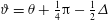 $\unicode[STIX]{x1D717}=\unicode[STIX]{x1D703}+\frac{1}{4}\unicode[STIX]{x03C0}-\frac{1}{2}\unicode[STIX]{x1D6E5}$
and so the pressure is
$\unicode[STIX]{x1D717}=\unicode[STIX]{x1D703}+\frac{1}{4}\unicode[STIX]{x03C0}-\frac{1}{2}\unicode[STIX]{x1D6E5}$
and so the pressure is
 $p=2Bi(\unicode[STIX]{x03C0}-\unicode[STIX]{x1D717})=Bi(\frac{3}{2}\unicode[STIX]{x03C0}-2\unicode[STIX]{x1D703}+\unicode[STIX]{x1D6E5})$
. In the
$p=2Bi(\unicode[STIX]{x03C0}-\unicode[STIX]{x1D717})=Bi(\frac{3}{2}\unicode[STIX]{x03C0}-2\unicode[STIX]{x1D703}+\unicode[STIX]{x1D6E5})$
. In the
 $x-y$
coordinate system, the force per unit length on this curve is
$x-y$
coordinate system, the force per unit length on this curve is
 $$\begin{eqnarray}\displaystyle \left[\begin{array}{@{}cc@{}}-p-Bi\sin 2\unicode[STIX]{x1D717} & Bi\cos 2\unicode[STIX]{x1D717}\\ Bi\cos 2\unicode[STIX]{x1D717} & -p+Bi\sin 2\unicode[STIX]{x1D717}\end{array}\right]\left[\begin{array}{@{}c@{}}\cos \unicode[STIX]{x1D703}\\ \sin \unicode[STIX]{x1D703}\end{array}\right], & & \displaystyle\end{eqnarray}$$
where
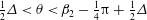 $\frac{1}{2}\unicode[STIX]{x1D6E5}<\unicode[STIX]{x1D703}<\unicode[STIX]{x1D6FD}_{2}-\frac{1}{4}\unicode[STIX]{x03C0}+\frac{1}{2}\unicode[STIX]{x1D6E5}$
. The horizontal force per unit length is
$\frac{1}{2}\unicode[STIX]{x1D6E5}<\unicode[STIX]{x1D703}<\unicode[STIX]{x1D6FD}_{2}-\frac{1}{4}\unicode[STIX]{x03C0}+\frac{1}{2}\unicode[STIX]{x1D6E5}$
. The horizontal force per unit length is
 $-p\cos \unicode[STIX]{x1D703}-Bi\cos (\unicode[STIX]{x1D6E5}-\unicode[STIX]{x1D703})$
, which can be integrated along
$-p\cos \unicode[STIX]{x1D703}-Bi\cos (\unicode[STIX]{x1D6E5}-\unicode[STIX]{x1D703})$
, which can be integrated along
 $EB$
to get the net horizontal force to be
$EB$
to get the net horizontal force to be
 $$\begin{eqnarray}\displaystyle \frac{F_{EB}}{Bi} & = & \displaystyle 2(\unicode[STIX]{x1D6FD}_{2}-\unicode[STIX]{x03C0})\sin \left(\unicode[STIX]{x1D6FD}_{2}-\frac{1}{4}\unicode[STIX]{x03C0}+\frac{1}{2}\unicode[STIX]{x1D6E5}\right)+\left(\frac{3}{2}\unicode[STIX]{x03C0}-1\right)\sin \frac{1}{2}\unicode[STIX]{x1D6E5}-\sin \left(\unicode[STIX]{x1D6FD}_{2}-\frac{1}{4}\unicode[STIX]{x03C0}-\frac{1}{2}\unicode[STIX]{x1D6E5}\right)\nonumber\\ \displaystyle & & \displaystyle +\,2\cos \left(\unicode[STIX]{x1D6FD}_{2}-\frac{1}{4}\unicode[STIX]{x03C0}+\frac{1}{2}\unicode[STIX]{x1D6E5}\right)-2\cos \frac{1}{2}\unicode[STIX]{x1D6E5}.\end{eqnarray}$$
Finally, on the surface
 $BC$
, the slipline angle is
$BC$
, the slipline angle is
 $\unicode[STIX]{x1D717}=\frac{1}{4}\unicode[STIX]{x03C0}$
and the pressure is
$\unicode[STIX]{x1D717}=\frac{1}{4}\unicode[STIX]{x03C0}$
and the pressure is
 $\frac{3}{2}\unicode[STIX]{x03C0}Bi$
. The horizontal force per unit length,
$\frac{3}{2}\unicode[STIX]{x03C0}Bi$
. The horizontal force per unit length,
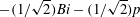 $-(1/\sqrt{2})Bi-(1/\sqrt{2})p$
, is then multiplied by the length of
$-(1/\sqrt{2})Bi-(1/\sqrt{2})p$
, is then multiplied by the length of
 $BC$
to obtain
$BC$
to obtain
 $$\begin{eqnarray}\displaystyle & \displaystyle \frac{F_{BC}}{Bi}=-\left(\frac{2+3\unicode[STIX]{x03C0}}{2\sqrt{2}}\right)(\unicode[STIX]{x1D706}-\sqrt{1-\unicode[STIX]{x1D706}^{2}}). & \displaystyle\end{eqnarray}$$
Combining (B 2), (B 4) and (B 5), we may compute
 $F_{x}=4(F_{EI}+F_{EB}+F_{BC})$
.
$F_{x}=4(F_{EI}+F_{EB}+F_{BC})$
.
B.2 Angular momentum balance
About any arbitrary origin, the two arcs of the rigidly rotating crescent
 $AEIE^{\prime }$
exert moments that must cancel in order to balance the net angular momentum of that plug. The cross product of momentum equations
$AEIE^{\prime }$
exert moments that must cancel in order to balance the net angular momentum of that plug. The cross product of momentum equations
 $\mathbf{0}=\unicode[STIX]{x1D735}\boldsymbol{\cdot }\unicode[STIX]{x1D748}$
, with the position vector
$\mathbf{0}=\unicode[STIX]{x1D735}\boldsymbol{\cdot }\unicode[STIX]{x1D748}$
, with the position vector
 $\boldsymbol{x}$
from that origin, followed by the integral over the crescent, implies
$\boldsymbol{x}$
from that origin, followed by the integral over the crescent, implies
 $$\begin{eqnarray}\displaystyle & \displaystyle 0=\int \int _{AEIE^{\prime }}\unicode[STIX]{x1D735}\boldsymbol{\cdot }(\boldsymbol{x}\times \unicode[STIX]{x1D748})\,\text{d}x\,\text{d}y=\int _{EAE^{\prime }}\boldsymbol{x}\times \unicode[STIX]{x1D748}\boldsymbol{\cdot }\boldsymbol{n}\,\text{d}\ell +\int _{EIE^{\prime }}\boldsymbol{x}\times \unicode[STIX]{x1D748}\boldsymbol{\cdot }\boldsymbol{n}\,\text{d}\ell , & \displaystyle\end{eqnarray}$$
where
 $\boldsymbol{n}$
is the outward normal to
$\boldsymbol{n}$
is the outward normal to
 $EAE^{\prime }$
and
$EAE^{\prime }$
and
 $EIE^{\prime }$
, and
$EIE^{\prime }$
, and
 $\text{d}\ell$
is the line element proceeding around the arcs in an anticlockwise sense with respect to the interior. That is,
$\text{d}\ell$
is the line element proceeding around the arcs in an anticlockwise sense with respect to the interior. That is,
 $$\begin{eqnarray}\displaystyle \displaystyle 0 & = & \displaystyle \int _{EIE^{\prime }}(\boldsymbol{x}-\boldsymbol{x}_{P})\times \unicode[STIX]{x1D748}\boldsymbol{\cdot }\boldsymbol{n}\,\text{d}\ell +\int _{EAE^{\prime }}(\boldsymbol{x}-\boldsymbol{x}_{O})\times \unicode[STIX]{x1D748}\boldsymbol{\cdot }\boldsymbol{n}\,\text{d}\ell \nonumber\\ \displaystyle & & \displaystyle +\,\boldsymbol{x}_{P}\times \int _{EIE^{\prime }}\unicode[STIX]{x1D748}\boldsymbol{\cdot }\boldsymbol{n}\,\text{d}\ell +\boldsymbol{x}_{O}\times \int _{EAE^{\prime }}\unicode[STIX]{x1D748}\boldsymbol{\cdot }\boldsymbol{n}\,\text{d}\ell ,\end{eqnarray}$$
where
 $\boldsymbol{x}_{P}$
and
$\boldsymbol{x}_{P}$
and
 $\boldsymbol{x}_{O}$
denote the positions of the centres of the circular arcs. But
$\boldsymbol{x}_{O}$
denote the positions of the centres of the circular arcs. But
 $\boldsymbol{x}_{P}-\boldsymbol{x}_{O}=(\unicode[STIX]{x1D706}/\sin \unicode[STIX]{x1D6FD}_{2})\hat{\boldsymbol{y}}$
and
$\boldsymbol{x}_{P}-\boldsymbol{x}_{O}=(\unicode[STIX]{x1D706}/\sin \unicode[STIX]{x1D6FD}_{2})\hat{\boldsymbol{y}}$
and
 $$\begin{eqnarray}\displaystyle & \displaystyle -\int _{EAE^{\prime }}\unicode[STIX]{x1D748}\boldsymbol{\cdot }\boldsymbol{n}\,\text{d}\ell =\int _{EIE^{\prime }}\unicode[STIX]{x1D748}\boldsymbol{\cdot }\boldsymbol{n}\,\text{d}\ell \equiv 2F_{EI}\hat{\boldsymbol{x}}, & \displaystyle\end{eqnarray}$$
given that the crescent must be in net force balance (which prescribes the net force on
 $EAE^{\prime }$
even though the full stress tensor is not known there). The angular momentum balance therefore implies
$EAE^{\prime }$
even though the full stress tensor is not known there). The angular momentum balance therefore implies
 $$\begin{eqnarray}\displaystyle & \displaystyle 0=T_{EIE^{\prime }}-T_{EAE^{\prime }}-2\frac{\unicode[STIX]{x1D706}F_{EI}}{\sin \unicode[STIX]{x1D6FD}_{2}}, & \displaystyle\end{eqnarray}$$
where
 $T_{EIE^{\prime }}$
and
$T_{EIE^{\prime }}$
and
 $T_{EAE^{\prime }}$
denote the torques on the arcs about their respective centres; i.e.
$T_{EAE^{\prime }}$
denote the torques on the arcs about their respective centres; i.e.
 $$\begin{eqnarray}\displaystyle T_{EIE^{\prime }}=\hat{\boldsymbol{z}}\boldsymbol{\cdot }\int _{EIE^{\prime }}(\boldsymbol{x}-\boldsymbol{x}_{P})\times \unicode[STIX]{x1D748}\boldsymbol{\cdot }\boldsymbol{n}\,\text{d}\ell =2r_{EI}^{2}\int _{\unicode[STIX]{x1D6FD}_{2}-\unicode[STIX]{x03C0}/2}^{\unicode[STIX]{x03C0}/2}(-Bi)\,\text{d}\unicode[STIX]{x1D703}_{p}, & & \displaystyle\end{eqnarray}$$
and
 $$\begin{eqnarray}\displaystyle T_{EAE^{\prime }}=\hat{\boldsymbol{z}}\boldsymbol{\cdot }\int _{EAE^{\prime }}(\boldsymbol{x}-\boldsymbol{x}_{O})\times \unicode[STIX]{x1D748}\boldsymbol{\cdot }\hat{\boldsymbol{r}}\,\text{d}\ell =2\int _{\unicode[STIX]{x1D703}_{E}}^{\unicode[STIX]{x03C0}/2}\unicode[STIX]{x1D71A}Bi\,\text{d}\unicode[STIX]{x1D703}, & & \displaystyle\end{eqnarray}$$
where
 $\hat{\boldsymbol{r}}$
is the radial unit vector and
$\hat{\boldsymbol{r}}$
is the radial unit vector and
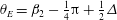 $\unicode[STIX]{x1D703}_{E}=\unicode[STIX]{x1D6FD}_{2}-\frac{1}{4}\unicode[STIX]{x03C0}+\frac{1}{2}\unicode[STIX]{x1D6E5}$
. Altogether (and after removing a factor of
$\unicode[STIX]{x1D703}_{E}=\unicode[STIX]{x1D6FD}_{2}-\frac{1}{4}\unicode[STIX]{x03C0}+\frac{1}{2}\unicode[STIX]{x1D6E5}$
. Altogether (and after removing a factor of
 $2Bi$
),
$2Bi$
),
 $$\begin{eqnarray}\displaystyle 0=r_{EI}^{2}(\unicode[STIX]{x03C0}-\unicode[STIX]{x1D6FD}_{2})+\unicode[STIX]{x1D71A}\left(\frac{1}{2}\unicode[STIX]{x03C0}-\unicode[STIX]{x1D703}_{E}\right)+\frac{\unicode[STIX]{x1D706}F_{EI}}{Bi\sin \unicode[STIX]{x1D6FD}_{2}}. & & \displaystyle\end{eqnarray}$$


