


1. Introduction
We examine turbulent stably stratified open channel flow as a canonical representation of flow in rivers and to some extent flow in estuaries and continental shelf seas. Where incident solar radiation penetrates the water column, the transmission and absorption of the radiation, following the Beer–Lambert law, can produce a stable thermocline near the free surface, whereas the near-wall region remains relatively unaffected by stratification. Relating the dynamics of the interior structure in these flows to known outer bulk parameters is very important. For example, in periods of drought or below average flow, Australian inland rivers can become thermally stratified to the extent that algal blooms may occur and oxygen or nutrient transport can be reduced, adversely affecting river biota and water quality. With reliable forecasting models these events may be predicted and mitigated against.
Simpson & Hunter (Reference Simpson and Hunter1974) proposed that in continental shelf seas, a constant fraction of the work done by tidal stresses acting on the seabed is available to mix the stratified surface layer and that this mechanical work can be compared with surface heat input to form a critical parameter for the onset of stratification. Similar interpretations have been proposed as a metric to delineate stratified and non-stratified flow regimes in estuaries (Holloway Reference Holloway1980), river flows (Bormans & Webster Reference Bormans and Webster1997) and in wind-induced surface mixing in the ocean (Kullenberg Reference Kullenberg1976; Simpson, Allen & Morris Reference Simpson, Allen and Morris1978). The total work input to the domain (
 ${\dot{W}}$
) and the rate at which potential energy (
${\dot{W}}$
) and the rate at which potential energy (
 $\dot{Ep}$
) must be increased to maintain a mixed column in steady conditions can be written
$\dot{Ep}$
) must be increased to maintain a mixed column in steady conditions can be written
 $$\begin{eqnarray}{\dot{W}}={\it\tau}_{w}u_{b}=u_{b}^{3}C_{f}\frac{1}{2}{\it\rho}_{0}={\it\rho}_{0}u_{{\it\tau}}^{3}\sqrt{\frac{2}{C_{f}}},\quad \dot{Ep}=\frac{g{\it\beta}}{C_{p}}{\it\delta}^{2}q_{N},\end{eqnarray}$$
where
 $C_{f}$
is the skin friction coefficient,
$C_{f}$
is the skin friction coefficient,
 $u_{b}$
is the bulk or volume-average velocity,
$u_{b}$
is the bulk or volume-average velocity,
 ${\it\rho}_{0}$
is the fluid density,
${\it\rho}_{0}$
is the fluid density,
 ${\it\tau}_{w}$
is the wall shear stress,
${\it\tau}_{w}$
is the wall shear stress,
 $u_{{\it\tau}}$
is the friction velocity,
$u_{{\it\tau}}$
is the friction velocity,
 $g$
is the gravitational acceleration,
$g$
is the gravitational acceleration,
 $C_{p}$
is the specific heat,
$C_{p}$
is the specific heat,
 ${\it\delta}$
is the domain height,
${\it\delta}$
is the domain height,
 ${\it\beta}$
is the coefficient of thermal expansion,
${\it\beta}$
is the coefficient of thermal expansion,
 $q(z)$
is the depth-varying volumetric heat source in the water column and
$q(z)$
is the depth-varying volumetric heat source in the water column and
 $$\begin{eqnarray}q_{N}=\frac{1}{{\it\delta}^{2}}\int _{0}^{{\it\delta}}(\overline{q}-q(z))(z-{\it\delta})\text{d}z,\quad \overline{q}=\frac{1}{{\it\delta}}\int _{0}^{{\it\delta}}q(z)\text{d}z.\end{eqnarray}$$
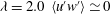
Combining (1.1a,b ) gives the ratio
 $$\begin{eqnarray}E_{r}=\frac{\dot{Ep}}{{\dot{W}}}=\frac{g{\it\beta}}{{\it\rho}_{0}C_{p}u_{{\it\tau}}^{3}}{\it\delta}^{2}q_{N}\sqrt{\frac{C_{f}}{2}}.\end{eqnarray}$$
In the setting shown in figure 1,
 $I_{s}$
is the radiant heat flux through the surface,
$I_{s}$
is the radiant heat flux through the surface,
 ${\it\alpha}$
is the absorption coefficient following the Beer–Lambert law, so
${\it\alpha}$
is the absorption coefficient following the Beer–Lambert law, so
 $$\begin{eqnarray}q(z)=I_{s}{\it\alpha}\text{e}^{({\it\delta}-z){\it\alpha}},\end{eqnarray}$$
and for large
 ${\it\alpha}{\it\delta}$
,
${\it\alpha}{\it\delta}$
,
 $E_{r}$
can be reduced to
$E_{r}$
can be reduced to
 $$\begin{eqnarray}E_{r}\simeq \frac{g{\it\beta}}{{\it\rho}_{0}C_{p}u_{{\it\tau}}^{3}}{\it\delta}I_{s}\biggl(\frac{1}{2}-\frac{1}{{\it\delta}{\it\alpha}}\biggr)\sqrt{\frac{C_{f}}{2}}.\end{eqnarray}$$
In coastal seas the critical values for the onset of stratification, determined by the location of seasonal thermal fronts, are typically
 $E_{rc}\simeq 0.003$
(Garrett, Keeley & Greenberg Reference Garrett, Keeley and Greenberg1978; Hearn Reference Hearn1985) for tidal mixing. Simpson & Hunter (Reference Simpson and Hunter1974) originally found
$E_{rc}\simeq 0.003$
(Garrett, Keeley & Greenberg Reference Garrett, Keeley and Greenberg1978; Hearn Reference Hearn1985) for tidal mixing. Simpson & Hunter (Reference Simpson and Hunter1974) originally found
 $E_{rc}=0.0037$
and Bormans & Webster (Reference Bormans and Webster1997) reported
$E_{rc}=0.0037$
and Bormans & Webster (Reference Bormans and Webster1997) reported
 $E_{rc}=0.0044$
in mixing in a river weir pool. It is not clear how the internal structure of the flow varies with the outer parameter
$E_{rc}=0.0044$
in mixing in a river weir pool. It is not clear how the internal structure of the flow varies with the outer parameter
 $E_{r}$
or how general
$E_{r}$
or how general
 $E_{rc}$
is across other parameters, Reynolds and Prandtl numbers
$E_{rc}$
is across other parameters, Reynolds and Prandtl numbers
 $Re$
,
$Re$
,
 $Pr$
, or
$Pr$
, or
 ${\it\alpha}{\it\beta}$
. These effects may be important at the reduced scale of some small river canals. It is clear that
${\it\alpha}{\it\beta}$
. These effects may be important at the reduced scale of some small river canals. It is clear that
 $E_{rc}$
is several orders of magnitude smaller than limit values of local flux Richardson number
$E_{rc}$
is several orders of magnitude smaller than limit values of local flux Richardson number
 $R_{f}$
, a measure of local mixing efficiency.
$R_{f}$
, a measure of local mixing efficiency.

Figure 1. Schematic of the flow; the domain is periodic in
 $x$
and
$x$
and
 $y$
.
$y$
.
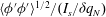
The influence of stratification in the atmospheric surface layer is characterised by the ratio of the Obukhov length scale
 $L=u_{{\it\tau}}^{3}/{\it\kappa}b_{\ast }$
, where
$L=u_{{\it\tau}}^{3}/{\it\kappa}b_{\ast }$
, where
 ${\it\kappa}$
is the von-Kaŕmań constant and
${\it\kappa}$
is the von-Kaŕmań constant and
 $b_{\ast }$
is the surface buoyancy flux, to a confinement scale which in the surface layer is
$b_{\ast }$
is the surface buoyancy flux, to a confinement scale which in the surface layer is
 $z$
(e.g. Monin Reference Monin1970; Chung & Matheou Reference Chung and Matheou2012). This ratio
$z$
(e.g. Monin Reference Monin1970; Chung & Matheou Reference Chung and Matheou2012). This ratio
 ${\it\zeta}=z/L$
indicates that the flow is affected by stratification for
${\it\zeta}=z/L$
indicates that the flow is affected by stratification for
 ${\it\zeta}\gtrsim 1$
, while for
${\it\zeta}\gtrsim 1$
, while for
 ${\it\zeta}\ll 1$
the flow approaches neutral conditions. For the current configuration, a bulk stability parameter
${\it\zeta}\ll 1$
the flow approaches neutral conditions. For the current configuration, a bulk stability parameter
 ${\it\lambda}$
(cf.
${\it\lambda}$
(cf.
 $E_{r}$
) can also be defined in terms of bulk Obukhov length scale
$E_{r}$
) can also be defined in terms of bulk Obukhov length scale
 $\mathscr{L}$
and confinement scale
$\mathscr{L}$
and confinement scale
 ${\it\delta}$
consistent with this approach and (1.5):
${\it\delta}$
consistent with this approach and (1.5):
 $$\begin{eqnarray}{\it\lambda}={\it\delta}/\mathscr{L},\quad \mathscr{L}=\frac{u_{{\it\tau}}^{3}}{g{\it\beta}I_{s}/{\it\rho}_{0}C_{p}}\biggl(\frac{1}{2}-\frac{1}{{\it\delta}{\it\alpha}}\biggr)^{-1}.\end{eqnarray}$$
Outside the surface layer the localised Obukhov length scale,
 ${\it\Lambda}(z)$
(Nieuwstadt Reference Nieuwstadt1984; Sorbjan Reference Sorbjan1986; Chung & Matheou Reference Chung and Matheou2012) can be defined in terms of fluxes as
${\it\Lambda}(z)$
(Nieuwstadt Reference Nieuwstadt1984; Sorbjan Reference Sorbjan1986; Chung & Matheou Reference Chung and Matheou2012) can be defined in terms of fluxes as
 $$\begin{eqnarray}{\it\zeta}(z)={\it\xi}/{\it\Lambda}(z),\quad {\it\Lambda}(z)=\langle u^{\prime }w^{\prime }\rangle ^{3/2}/\langle b^{\prime }w^{\prime }\rangle ,\end{eqnarray}$$
where
 ${\it\xi}$
is a local confinement scale such as
${\it\xi}$
is a local confinement scale such as
 $z$
, the buoyancy fluctuation is
$z$
, the buoyancy fluctuation is
 $b^{\prime }=g{\it\rho}^{\prime }/{\it\rho}_{0}$
,
$b^{\prime }=g{\it\rho}^{\prime }/{\it\rho}_{0}$
,
 $\langle \,\rangle$
denotes temporal averaging and the prime denotes a perturbation from the mean. Recent efforts to parameterise the effects of stratification on mixing in turbulent flow (Ivey & Imberger Reference Ivey and Imberger1991; Holt, Koseff & Ferziger Reference Holt, Koseff and Ferziger1992; Itsweire et al.
Reference Itsweire, Koseff, Briggs and Ferziger1993; Barry et al.
Reference Barry, Ivey, Winters and Imberger2001; Shih et al.
Reference Shih, Koseff, Ivey and Ferziger2005; Lindborg Reference Lindborg2006; Brethouwer et al.
Reference Brethouwer, Billant, Lindborg and Chomaz2007; Gonzalez-Juez, Kerstein & Shih Reference Gonzalez-Juez, Kerstein and Shih2011; Chung & Matheou Reference Chung and Matheou2012) have demonstrated that multiple regimes of behaviour exist, which can be related to two non-dimensional parameters: the buoyancy Reynolds number
$\langle \,\rangle$
denotes temporal averaging and the prime denotes a perturbation from the mean. Recent efforts to parameterise the effects of stratification on mixing in turbulent flow (Ivey & Imberger Reference Ivey and Imberger1991; Holt, Koseff & Ferziger Reference Holt, Koseff and Ferziger1992; Itsweire et al.
Reference Itsweire, Koseff, Briggs and Ferziger1993; Barry et al.
Reference Barry, Ivey, Winters and Imberger2001; Shih et al.
Reference Shih, Koseff, Ivey and Ferziger2005; Lindborg Reference Lindborg2006; Brethouwer et al.
Reference Brethouwer, Billant, Lindborg and Chomaz2007; Gonzalez-Juez, Kerstein & Shih Reference Gonzalez-Juez, Kerstein and Shih2011; Chung & Matheou Reference Chung and Matheou2012) have demonstrated that multiple regimes of behaviour exist, which can be related to two non-dimensional parameters: the buoyancy Reynolds number
 $\mathscr{R}$
(Dillon & Caldwell Reference Dillon and Caldwell1980; Gargett, Osborn & Nasmyth Reference Gargett, Osborn and Nasmyth1984; Itsweire et al.
Reference Itsweire, Koseff, Briggs and Ferziger1993) and the gradient Richardson number
$\mathscr{R}$
(Dillon & Caldwell Reference Dillon and Caldwell1980; Gargett, Osborn & Nasmyth Reference Gargett, Osborn and Nasmyth1984; Itsweire et al.
Reference Itsweire, Koseff, Briggs and Ferziger1993) and the gradient Richardson number
 $Ri$
,
$Ri$
,
 $$\begin{eqnarray}\mathscr{R}=\frac{{\it\epsilon}}{{\it\nu}N^{2}}=\biggl(\frac{l_{O}}{{\it\eta}}\biggr)^{4/3},\quad Ri=\frac{N^{2}}{S^{2}}=\biggl(\frac{l_{C}}{l_{O}}\biggr)^{4/3}.\end{eqnarray}$$
These parameters can be formed out of characteristic length scales in stratified turbulent flow (Smyth & Moum Reference Smyth and Moum2000; Brethouwer et al.
Reference Brethouwer, Billant, Lindborg and Chomaz2007; Chung & Matheou Reference Chung and Matheou2012): the Ozmidov length scale
 $l_{O}$
, the length scale above which the effects of buoyancy are strongly felt; the Kolmogorov length scale
$l_{O}$
, the length scale above which the effects of buoyancy are strongly felt; the Kolmogorov length scale
 ${\it\eta}$
, which characterises the smallest scales of motion; and the Corrsin scale
${\it\eta}$
, which characterises the smallest scales of motion; and the Corrsin scale
 $l_{C}$
, the length scale characterising the smallest eddies which interact with background shear,
$l_{C}$
, the length scale characterising the smallest eddies which interact with background shear,
 $$\begin{eqnarray}l_{C}=\biggl(\frac{{\it\epsilon}}{S^{3}}\biggr)^{1/2},\quad l_{O}=\biggl(\frac{{\it\epsilon}}{N^{3}}\biggr)^{1/2},\quad {\it\eta}=\biggl(\frac{{\it\nu}^{3}}{{\it\epsilon}}\biggr)^{1/4},\end{eqnarray}$$
where
 $N^{2}=(-g/{\it\rho})(\text{d}\langle {\it\rho}\rangle /\text{d}z)$
,
$N^{2}=(-g/{\it\rho})(\text{d}\langle {\it\rho}\rangle /\text{d}z)$
,
 $S=(\text{d}\langle U\rangle /\text{d}z)$
, the turbulent dissipation rate
$S=(\text{d}\langle U\rangle /\text{d}z)$
, the turbulent dissipation rate
 ${\it\epsilon}={\it\nu}\langle (\partial u_{i}^{\prime }/\partial x_{j})^{2}\rangle$
and
${\it\epsilon}={\it\nu}\langle (\partial u_{i}^{\prime }/\partial x_{j})^{2}\rangle$
and
 ${\it\nu}$
is the kinematic viscosity.
${\it\nu}$
is the kinematic viscosity.
In the limit
 $Ri\rightarrow 0$
,
$Ri\rightarrow 0$
,
 $l_{O}\gg l_{C}$
, the flow approaches neutral conditions and the flow is characterised by
$l_{O}\gg l_{C}$
, the flow approaches neutral conditions and the flow is characterised by
 $l_{C}$
and
$l_{C}$
and
 ${\it\eta}$
(Smyth & Moum Reference Smyth and Moum2000). With increasing stability (decreasing
${\it\eta}$
(Smyth & Moum Reference Smyth and Moum2000). With increasing stability (decreasing
 $l_{O}$
), for
$l_{O}$
), for
 $l_{O}>l_{C}>{\it\eta}$
, the flow approaches a regime of constant, maximum mixing efficiency and
$l_{O}>l_{C}>{\it\eta}$
, the flow approaches a regime of constant, maximum mixing efficiency and
 $Ri$
approaches a critical value
$Ri$
approaches a critical value
 $Ri_{c}\simeq 0.2{-}0.25$
(Holt et al.
Reference Holt, Koseff and Ferziger1992; Chung & Matheou Reference Chung and Matheou2012). Scales between
$Ri_{c}\simeq 0.2{-}0.25$
(Holt et al.
Reference Holt, Koseff and Ferziger1992; Chung & Matheou Reference Chung and Matheou2012). Scales between
 $l_{O}$
and
$l_{O}$
and
 ${\it\eta}$
are weakly affected by stratification while those larger than
${\it\eta}$
are weakly affected by stratification while those larger than
 $l_{O}$
are strongly affected, leading to modification of the classical energy cascade in turbulent flow (Lindborg Reference Lindborg2006; Brethouwer et al.
Reference Brethouwer, Billant, Lindborg and Chomaz2007). Further, with increasing stability the flow approaches a regime where buoyancy affects the smallest scales of motions (Brethouwer et al.
Reference Brethouwer, Billant, Lindborg and Chomaz2007) and turbulent mixing is strongly suppressed by buoyancy (Itsweire et al.
Reference Itsweire, Koseff, Briggs and Ferziger1993; Barry et al.
Reference Barry, Ivey, Winters and Imberger2001; Shih et al.
Reference Shih, Koseff, Ivey and Ferziger2005; Brethouwer et al.
Reference Brethouwer, Billant, Lindborg and Chomaz2007; Ivey, Winters & Koseff Reference Ivey, Winters and Koseff2008; Gonzalez-Juez et al.
Reference Gonzalez-Juez, Kerstein and Shih2011). Brethouwer et al. (Reference Brethouwer, Billant, Lindborg and Chomaz2007) found
$l_{O}$
are strongly affected, leading to modification of the classical energy cascade in turbulent flow (Lindborg Reference Lindborg2006; Brethouwer et al.
Reference Brethouwer, Billant, Lindborg and Chomaz2007). Further, with increasing stability the flow approaches a regime where buoyancy affects the smallest scales of motions (Brethouwer et al.
Reference Brethouwer, Billant, Lindborg and Chomaz2007) and turbulent mixing is strongly suppressed by buoyancy (Itsweire et al.
Reference Itsweire, Koseff, Briggs and Ferziger1993; Barry et al.
Reference Barry, Ivey, Winters and Imberger2001; Shih et al.
Reference Shih, Koseff, Ivey and Ferziger2005; Brethouwer et al.
Reference Brethouwer, Billant, Lindborg and Chomaz2007; Ivey, Winters & Koseff Reference Ivey, Winters and Koseff2008; Gonzalez-Juez et al.
Reference Gonzalez-Juez, Kerstein and Shih2011). Brethouwer et al. (Reference Brethouwer, Billant, Lindborg and Chomaz2007) found
 $\mathscr{R}_{c}\simeq 1$
a sufficient criterion for the onset of this behaviour. In the atmospheric surface layer, the collapse of turbulence was found by Flores & Riley (Reference Flores and Riley2011) to be characterised by a related parameter
$\mathscr{R}_{c}\simeq 1$
a sufficient criterion for the onset of this behaviour. In the atmospheric surface layer, the collapse of turbulence was found by Flores & Riley (Reference Flores and Riley2011) to be characterised by a related parameter
 $L_{\ast }=Lu_{{\it\tau}}/{\it\nu}$
in the terms of the Obukhov length scale, and found a critical limit of
$L_{\ast }=Lu_{{\it\tau}}/{\it\nu}$
in the terms of the Obukhov length scale, and found a critical limit of
 $L_{\ast ,c}\lesssim 100$
.
$L_{\ast ,c}\lesssim 100$
.
The description of the state of stratified turbulence then requires an outer buoyancy parameter, such as
 $Ri$
or
$Ri$
or
 ${\it\lambda}$
, and a parameter related to
${\it\lambda}$
, and a parameter related to
 ${\it\nu}$
, such as
${\it\nu}$
, such as
 $\mathscr{R}$
or
$\mathscr{R}$
or
 $L_{\ast }$
(Chung & Matheou Reference Chung and Matheou2012). For the present flow the equivalent definitions of
$L_{\ast }$
(Chung & Matheou Reference Chung and Matheou2012). For the present flow the equivalent definitions of
 $L_{\ast }$
for bulk and local parameters can be defined as
$L_{\ast }$
for bulk and local parameters can be defined as
 $$\begin{eqnarray}Re_{\mathscr{L}}=\mathscr{L}u_{{\it\tau}}/{\it\nu},\quad Re_{{\it\Lambda}}(z)={\it\Lambda}\langle u^{\prime }w^{\prime }\rangle ^{1/2}/{\it\nu}.\end{eqnarray}$$
We then define our problem, as outlined in figure 1, in terms of the parameter set
 $({\it\alpha}{\it\delta},{\it\lambda},Re_{{\it\tau}},Pr)$
with the friction Reynolds number
$({\it\alpha}{\it\delta},{\it\lambda},Re_{{\it\tau}},Pr)$
with the friction Reynolds number
 $Re_{{\it\tau}}=u_{{\it\tau}}{\it\delta}/{\it\nu}$
, or equivalently the set
$Re_{{\it\tau}}=u_{{\it\tau}}{\it\delta}/{\it\nu}$
, or equivalently the set
 $({\it\alpha}{\it\delta},{\it\lambda},Re_{\mathscr{L}},Pr)$
with
$({\it\alpha}{\it\delta},{\it\lambda},Re_{\mathscr{L}},Pr)$
with
 $Re_{\mathscr{L}}\equiv Re_{{\it\tau}}/{\it\lambda}$
. We have acknowledged a Prandtl number dependence (Barry et al.
Reference Barry, Ivey, Winters and Imberger2001; Shih et al.
Reference Shih, Koseff, Ivey and Ferziger2005; Gonzalez-Juez et al.
Reference Gonzalez-Juez, Kerstein and Shih2011) here but confine our study to fixed
$Re_{\mathscr{L}}\equiv Re_{{\it\tau}}/{\it\lambda}$
. We have acknowledged a Prandtl number dependence (Barry et al.
Reference Barry, Ivey, Winters and Imberger2001; Shih et al.
Reference Shih, Koseff, Ivey and Ferziger2005; Gonzalez-Juez et al.
Reference Gonzalez-Juez, Kerstein and Shih2011) here but confine our study to fixed
 $Pr=0.71$
. The objective of the study is to examine how local flow character varies with these bulk parameters and in terms of the local parameters defined in (1.8).
$Pr=0.71$
. The objective of the study is to examine how local flow character varies with these bulk parameters and in terms of the local parameters defined in (1.8).
We describe our method in § 2 and in § 3 we show that we are able to attain a statistically steady flow field over a wide range of stability ratios and, unlike most previous studies, the near-wall region remains only very weakly affected by buoyancy. In § 4.1 we show that
 ${\it\lambda}\simeq 1$
indicates a transition to strongly stratified flow and for
${\it\lambda}\simeq 1$
indicates a transition to strongly stratified flow and for
 ${\it\lambda}\gtrsim 1$
the flow is in local energetic equilibrium. In § 4.2 we show that
${\it\lambda}\gtrsim 1$
the flow is in local energetic equilibrium. In § 4.2 we show that
 $Re_{\mathscr{L}}\simeq 200{-}400$
is associated with the onset of the weakly turbulent
$Re_{\mathscr{L}}\simeq 200{-}400$
is associated with the onset of the weakly turbulent
 $\mathscr{R}<\mathscr{R}_{c}$
regime in the outer boundary layer and that the onset of local equilibrium conditions allows a direct relationship between
$\mathscr{R}<\mathscr{R}_{c}$
regime in the outer boundary layer and that the onset of local equilibrium conditions allows a direct relationship between
 $\mathscr{R}$
and
$\mathscr{R}$
and
 $Re_{{\it\Lambda}}(z)$
to be obtained. In § 4.3 we conclude that the parameter set (
$Re_{{\it\Lambda}}(z)$
to be obtained. In § 4.3 we conclude that the parameter set (
 ${\it\lambda}$
,
${\it\lambda}$
,
 $Re_{\mathscr{L}}$
) is more relevant for describing the dynamics of the flow than
$Re_{\mathscr{L}}$
) is more relevant for describing the dynamics of the flow than
 $E_{r}$
. In § 4.4 we identify these transition behaviours in terms of the turbulent eddy viscosity
$E_{r}$
. In § 4.4 we identify these transition behaviours in terms of the turbulent eddy viscosity
 $k_{m}$
. The outer extremities of the channel – the near-wall region and the free surface – impose other length scale restrictions on the flow. In § 5 we examine the scaling for
$k_{m}$
. The outer extremities of the channel – the near-wall region and the free surface – impose other length scale restrictions on the flow. In § 5 we examine the scaling for
 $\mathscr{R}$
in the near-wall region and show that
$\mathscr{R}$
in the near-wall region and show that
 $\mathscr{R}\sim Re_{\mathscr{L}}Re_{{\it\tau}}$
, rather than the
$\mathscr{R}\sim Re_{\mathscr{L}}Re_{{\it\tau}}$
, rather than the
 $\mathscr{R}\sim Re_{\mathscr{L}}$
which holds in stratified boundary layer flows where the buoyancy flux is non-zero at the wall, leading to a wider separation of viscous- and buoyancy-affected scales at the wall in the present configuration. In § 6 we consider the modifications to the scaling for the length of the near-free-surface affected region under stratified conditions.
$\mathscr{R}\sim Re_{\mathscr{L}}$
which holds in stratified boundary layer flows where the buoyancy flux is non-zero at the wall, leading to a wider separation of viscous- and buoyancy-affected scales at the wall in the present configuration. In § 6 we consider the modifications to the scaling for the length of the near-free-surface affected region under stratified conditions.
2. Problem formulation
We approach this problem by obtaining a numerical simulation of the flow illustrated in figure 1. The flow is periodic in the horizontal plane and driven by a constant pressure gradient. A volumetric heat source, following (1.4), is applied to the flow. In our canonical model we assume no heat is lost through the lower wall or the stress-free surface, which are taken as adiabatic. After an initial transient period the flow attains a statistically steady horizontally homogeneous state and the energy input from the source term is transported across the channel at a constant rate, so the dimensional temperature field
 ${\it\Phi}$
at time
${\it\Phi}$
at time
 $T$
can be decomposed into
$T$
can be decomposed into
 $$\begin{eqnarray}{\it\Phi}(\mathbf{x},T)={\it\Phi}^{\prime }(\mathbf{x},T)+\overline{{\it\Phi}}(T),\end{eqnarray}$$
where
 ${\it\Phi}^{\prime }$
is the statistically steady temperature field and the uniform increase in temperature with time is
${\it\Phi}^{\prime }$
is the statistically steady temperature field and the uniform increase in temperature with time is
 $$\begin{eqnarray}\partial \overline{{\it\Phi}}/\partial T=\overline{q}/{\it\rho}_{0}C_{p}.\end{eqnarray}$$
With this reference frame we obtain a non-dimensional statistically steady temperature field (
 ${\it\phi}$
) and depth-varying heat source (
${\it\phi}$
) and depth-varying heat source (
 $qe$
) by normalising
$qe$
) by normalising
 ${\it\Phi}_{N}=q_{N}{\it\delta}/{\it\rho}_{0}C_{p}u_{{\it\tau}}$
and
${\it\Phi}_{N}=q_{N}{\it\delta}/{\it\rho}_{0}C_{p}u_{{\it\tau}}$
and
 $q_{N}$
(defined in (1.2)) respectively,
$q_{N}$
(defined in (1.2)) respectively,
 $$\begin{eqnarray}{\it\phi}=\frac{({\it\Phi}-\overline{{\it\Phi}}(T))}{{\it\Phi}_{N}},\quad qe(z)=\frac{(q(z)-\overline{q})}{q_{N}}.\end{eqnarray}$$
With this normalisation we perform direct numerical simulations (DNS) of the Navier–Stokes equations. We consider an incompressible fluid with the Oberbeck–Boussinesq approximation for buoyancy. The governing equations for the conservation of mass, momentum and energy are written in non-dimensional form as
 $$\begin{eqnarray}\displaystyle & \displaystyle \boldsymbol{{\rm\nabla}}\boldsymbol{\cdot }\boldsymbol{u}=0, & \displaystyle\end{eqnarray}$$
 $$\begin{eqnarray}\displaystyle & \displaystyle \frac{\partial \boldsymbol{u}}{\partial t}+\boldsymbol{{\rm\nabla}}\boldsymbol{\cdot }(\boldsymbol{uu})=-\boldsymbol{{\rm\nabla}}p+\frac{1}{Re_{{\it\tau}}}{\rm\nabla}^{2}\boldsymbol{u}+\boldsymbol{e}_{x}+{\it\lambda}{\it\phi}\boldsymbol{e}_{z}, & \displaystyle\end{eqnarray}$$
 $$\begin{eqnarray}\frac{\partial {\it\phi}}{\partial t}+\boldsymbol{{\rm\nabla}}\boldsymbol{\cdot }(\boldsymbol{u}{\it\phi})=\frac{1}{Re_{{\it\tau}}Pr}{\rm\nabla}^{2}{\it\phi}+qe,\end{eqnarray}$$
where
 $\boldsymbol{e}_{x}$
and
$\boldsymbol{e}_{x}$
and
 $\boldsymbol{e}_{z}$
are the unit vectors in the
$\boldsymbol{e}_{z}$
are the unit vectors in the
 $x$
and
$x$
and
 $z$
directions. The Prandtl number
$z$
directions. The Prandtl number
 $Pr={\it\nu}/{\it\sigma}=0.71$
, where
$Pr={\it\nu}/{\it\sigma}=0.71$
, where
 ${\it\sigma}$
is the scalar diffusivity of the fluid. With this non-dimensional form, the velocity field is normalised by
${\it\sigma}$
is the scalar diffusivity of the fluid. With this non-dimensional form, the velocity field is normalised by
 $u_{{\it\tau}}$
which is set through the specified
$u_{{\it\tau}}$
which is set through the specified
 $Re_{{\it\tau}}=u_{{\it\tau}}{\it\delta}/{\it\nu}$
and the constant imposed pressure gradient in the streamwise direction,
$Re_{{\it\tau}}=u_{{\it\tau}}{\it\delta}/{\it\nu}$
and the constant imposed pressure gradient in the streamwise direction,
 $\boldsymbol{e}_{x}$
. The length, time and pressure are made non-dimensional by
$\boldsymbol{e}_{x}$
. The length, time and pressure are made non-dimensional by
 ${\it\delta}$
,
${\it\delta}$
,
 $u_{{\it\tau}}$
and
$u_{{\it\tau}}$
and
 ${\it\rho}_{0}$
, a reference density. In specifying the problem,
${\it\rho}_{0}$
, a reference density. In specifying the problem,
 $Re_{{\it\tau}}$
and
$Re_{{\it\tau}}$
and
 ${\it\lambda}$
are given and, together with
${\it\lambda}$
are given and, together with
 ${\it\alpha}{\it\delta}$
(specified in (1.4)) and
${\it\alpha}{\it\delta}$
(specified in (1.4)) and
 $Pr$
, fully describe the problem. In this scheme the surface flux
$Pr$
, fully describe the problem. In this scheme the surface flux
 $I_{s}$
which occurs in (1.4) is a free variable which scales the temperature field. In presenting the results, we re-normalise the temperature field by either
$I_{s}$
which occurs in (1.4) is a free variable which scales the temperature field. In presenting the results, we re-normalise the temperature field by either
 $I_{s}$
or the bulk temperature difference
$I_{s}$
or the bulk temperature difference
 ${\rm\Delta}{\it\phi}={\it\phi}_{1}-{\it\phi}_{0}$
, where
${\rm\Delta}{\it\phi}={\it\phi}_{1}-{\it\phi}_{0}$
, where
 ${\it\phi}_{1}$
and
${\it\phi}_{1}$
and
 ${\it\phi}_{0}$
are the free-surface and wall temperatures respectively. This gives more meaningful normalisation of
${\it\phi}_{0}$
are the free-surface and wall temperatures respectively. This gives more meaningful normalisation of
 ${\it\phi}_{d}={\it\phi}/{\rm\Delta}{\it\phi}$
or
${\it\phi}_{d}={\it\phi}/{\rm\Delta}{\it\phi}$
or
 ${\it\phi}_{i}={\it\phi}/(I_{s}/{\it\delta}q_{N})$
.
${\it\phi}_{i}={\it\phi}/(I_{s}/{\it\delta}q_{N})$
.
The boundary conditions for the bottom (
 $z=0$
) no-slip adiabatic wall and stress-free adiabatic top boundary (
$z=0$
) no-slip adiabatic wall and stress-free adiabatic top boundary (
 $z=1$
) are
$z=1$
) are
 $$\begin{eqnarray}\displaystyle & \displaystyle z=0:\quad u=v=w=0,\quad \frac{\partial {\it\phi}}{\partial z}=0, & \displaystyle\end{eqnarray}$$
 $$\begin{eqnarray}\displaystyle & \displaystyle z=1:\quad \frac{\partial u}{\partial z}=\frac{\partial v}{\partial z}=w=0,\quad \frac{\partial {\it\phi}}{\partial z}=0. & \displaystyle\end{eqnarray}$$
2.1. DNS
The equations are solved using the fractional-step finite-volume solver described in Armfield et al. (Reference Armfield, Norris, Morgan and Street2002). The code uses a cell-centred co-located storage arrangement for flow variables on a regular structured grid, with cell-face velocities calculated using the Rhie–Chow momentum interpolation. The spatial derivatives are discretised using second-order central finite differences. A second-order-accurate Adams–Bashforth time advancement scheme is used for the nonlinear terms and Crank–Nicolson for the time advancement of the diffusive terms. The pressure correction equation is solved using a stabilised bi-conjugate gradient solver with an incomplete Cholesky factorisation pre-conditioner. The momentum and temperature equations are solved using a Jacobi solver. A Courant number limit of 0.2–0.24 is used to obtain the time step size.
The simulation parameters are given in table 1. We perform simulations from neutral (
 ${\it\lambda}=0$
) to stable conditions (
${\it\lambda}=0$
) to stable conditions (
 ${\it\lambda}=0.05{-}2.0$
) at
${\it\lambda}=0.05{-}2.0$
) at
 $Re_{{\it\tau}}=395$
and
$Re_{{\it\tau}}=395$
and
 ${\it\alpha}{\it\delta}=8$
. We demonstrate a sufficient range to determine the transition to a high-
${\it\alpha}{\it\delta}=8$
. We demonstrate a sufficient range to determine the transition to a high-
 ${\it\lambda}$
flow structure where critical values of
${\it\lambda}$
flow structure where critical values of
 $Ri$
are achieved in the channel core and the turbulent kinetic energy (TKE) balance is in local equilibrium. Additional simulations are performed at higher and lower Reynolds number
$Ri$
are achieved in the channel core and the turbulent kinetic energy (TKE) balance is in local equilibrium. Additional simulations are performed at higher and lower Reynolds number
 $Re_{{\it\tau}}=200{-}800$
and at
$Re_{{\it\tau}}=200{-}800$
and at
 ${\it\alpha}{\it\delta}=32$
. Unless otherwise stated, results are for
${\it\alpha}{\it\delta}=32$
. Unless otherwise stated, results are for
 $Re_{{\it\tau}}=395$
,
$Re_{{\it\tau}}=395$
,
 ${\it\alpha}{\it\delta}=8$
.
${\it\alpha}{\it\delta}=8$
.
The Kolmogorov length scale, expressed in viscous wall units
 ${\it\eta}^{+}=Re_{{\it\tau}}{\it\eta}/{\it\delta}$
, ranges over
${\it\eta}^{+}=Re_{{\it\tau}}{\it\eta}/{\it\delta}$
, ranges over
 ${\it\eta}^{+}=1.5{-}4.7$
(shown in § 5). At
${\it\eta}^{+}=1.5{-}4.7$
(shown in § 5). At
 $Re_{{\it\tau}}=395$
, the grid size is set at
$Re_{{\it\tau}}=395$
, the grid size is set at
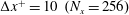 ${\rm\Delta}x^{+}=10~(N_{x}=256)$
,
${\rm\Delta}x^{+}=10~(N_{x}=256)$
,
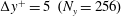 ${\rm\Delta}y^{+}=5~(N_{y}=256)$
for
${\rm\Delta}y^{+}=5~(N_{y}=256)$
for
 ${\it\lambda}=0{-}0.5$
. In the vertical axis, the grid is stretched from
${\it\lambda}=0{-}0.5$
. In the vertical axis, the grid is stretched from
 ${\rm\Delta}z^{+}=0.4$
at the wall to
${\rm\Delta}z^{+}=0.4$
at the wall to
 ${\rm\Delta}z^{+}=3.95$
at
${\rm\Delta}z^{+}=3.95$
at
 $z=0.6$
and from
$z=0.6$
and from
 $z=0.6{-}1$
the grid is uniform with
$z=0.6{-}1$
the grid is uniform with
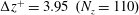 ${\rm\Delta}z^{+}=3.95~(N_{z}=110)$
. At
${\rm\Delta}z^{+}=3.95~(N_{z}=110)$
. At
 ${\it\lambda}=1.0{-}2.0$
the grid was refined to
${\it\lambda}=1.0{-}2.0$
the grid was refined to
 ${\rm\Delta}x^{+}=4.68~(N_{x}=540)$
and in the vertical
${\rm\Delta}x^{+}=4.68~(N_{x}=540)$
and in the vertical
 ${\rm\Delta}z^{+}=0.4{-}4.1$
with the grid stretched to
${\rm\Delta}z^{+}=0.4{-}4.1$
with the grid stretched to
 ${\rm\Delta}z^{+}=1.1$
at the free surface (
${\rm\Delta}z^{+}=1.1$
at the free surface (
 $N_{z}=130$
). At
$N_{z}=130$
). At
 ${\it\alpha}{\it\delta}=32$
, this vertical resolution is also used. The single simulation at
${\it\alpha}{\it\delta}=32$
, this vertical resolution is also used. The single simulation at
 $Re_{{\it\tau}}=800$
has
$Re_{{\it\tau}}=800$
has
 ${\rm\Delta}x^{+}=10$
,
${\rm\Delta}x^{+}=10$
,
 ${\rm\Delta}y^{+}=5$
and
${\rm\Delta}y^{+}=5$
and
 ${\rm\Delta}z^{+}=0.4{-}4.0$
. The accuracy of the results has been verified in neutral conditions against benchmark DNS solutions of Abe, Kawamura & Matsuo (Reference Abe, Kawamura and Matsuo2001) and Moser, Kim & Mansour (Reference Moser, Kim and Mansour1999) for closed channel flow at
${\rm\Delta}z^{+}=0.4{-}4.0$
. The accuracy of the results has been verified in neutral conditions against benchmark DNS solutions of Abe, Kawamura & Matsuo (Reference Abe, Kawamura and Matsuo2001) and Moser, Kim & Mansour (Reference Moser, Kim and Mansour1999) for closed channel flow at
 $Re=395$
.
$Re=395$
.
Initial simulations were performed at neutral conditions. After an initial transient phase, typically
 ${\rm\Delta}t=30{-}40$
(non-dimensional time units
${\rm\Delta}t=30{-}40$
(non-dimensional time units
 ${\it\delta}/Tu_{{\it\tau}}$
), statistically steady conditions were judged to have been obtained. This was determined by convergence of zeroth- and second-order moments of temperature and velocity fluctuations to the mean values and balance of the transport budget for
${\it\delta}/Tu_{{\it\tau}}$
), statistically steady conditions were judged to have been obtained. This was determined by convergence of zeroth- and second-order moments of temperature and velocity fluctuations to the mean values and balance of the transport budget for
 ${\it\phi}$
(see (3.1) below) over the height of the domain. The flow was then evolved for a further period, typically
${\it\phi}$
(see (3.1) below) over the height of the domain. The flow was then evolved for a further period, typically
 ${\rm\Delta}t=40{-}80$
, with statistics collected. Subsequent higher
${\rm\Delta}t=40{-}80$
, with statistics collected. Subsequent higher
 ${\it\lambda}$
flow conditions were successively initialised from these converged solution flow fields and computations continued in the same manner.
${\it\lambda}$
flow conditions were successively initialised from these converged solution flow fields and computations continued in the same manner.
3. Temperature stratification profile
A defining feature of this flow is the separation of the stratified outer layer from the near-wall region so that even at large bulk stability ratio,
 ${\it\lambda}$
, turbulence production at the wall remains relatively unaffected by buoyancy. In this section we examine this flow structure with reference to the vertical profiles of mean flow statistics, obtained in statistically steady conditions and averaged over a horizontal plane and in time, as denoted by
${\it\lambda}$
, turbulence production at the wall remains relatively unaffected by buoyancy. In this section we examine this flow structure with reference to the vertical profiles of mean flow statistics, obtained in statistically steady conditions and averaged over a horizontal plane and in time, as denoted by
 $\langle \cdot \rangle$
.
$\langle \cdot \rangle$
.

Figure 2. Mean temperature profile,
 $({\it\phi}-{\it\phi}_{0})/(I_{s}/{\it\delta}q_{N})$
at
$({\it\phi}-{\it\phi}_{0})/(I_{s}/{\it\delta}q_{N})$
at
 $\mathit{Re}_{{\it\tau}}=395$
,
$\mathit{Re}_{{\it\tau}}=395$
,
 ${\it\alpha}{\it\delta}=8$
(a) and
${\it\alpha}{\it\delta}=8$
(a) and
 $\mathit{Re}_{{\it\tau}}=200{-}800$
,
$\mathit{Re}_{{\it\tau}}=200{-}800$
,
 ${\it\alpha}{\it\delta}=8{-}32$
(b).
${\it\alpha}{\it\delta}=8{-}32$
(b).
Table 1. Simulation parameters, and measured flow statistics:
 $E_{r}={\it\lambda}\sqrt{C_{f}/2}$
,
$E_{r}={\it\lambda}\sqrt{C_{f}/2}$
,
 $C_{f}=2(u_{{\it\tau}}/u_{b})^{2}$
,
$C_{f}=2(u_{{\it\tau}}/u_{b})^{2}$
,
 $Ri_{b}={\rm\Delta}{\it\phi}{\it\lambda}{\it\delta}/u_{b}^{2}$
,
$Ri_{b}={\rm\Delta}{\it\phi}{\it\lambda}{\it\delta}/u_{b}^{2}$
,
 $Ri_{{\it\tau}}={\rm\Delta}{\it\phi}{\it\lambda}{\it\delta}/u_{{\it\tau}}^{2}$
, and
$Ri_{{\it\tau}}={\rm\Delta}{\it\phi}{\it\lambda}{\it\delta}/u_{{\it\tau}}^{2}$
, and
 $Re_{{\it\tau}}^{\ast }$
is Reynolds number based on the measured wall friction velocity
$Re_{{\it\tau}}^{\ast }$
is Reynolds number based on the measured wall friction velocity
 $u_{{\it\tau}}^{\ast }$
.
$u_{{\it\tau}}^{\ast }$
.

The mean temperature profile normalised by the incident surface flux
 $(I_{s}/{\it\delta}q_{N})$
is shown in figure 2(a) for flow at
$(I_{s}/{\it\delta}q_{N})$
is shown in figure 2(a) for flow at
 $Re_{{\it\tau}}=395$
,
$Re_{{\it\tau}}=395$
,
 ${\it\alpha}{\it\delta}=8$
and
${\it\alpha}{\it\delta}=8$
and
 ${\it\lambda}=0{-}2.0$
while in figure 2(b) the results are compared with flow at
${\it\lambda}=0{-}2.0$
while in figure 2(b) the results are compared with flow at
 ${\it\lambda}=0.5$
,
${\it\lambda}=0.5$
,
 ${\it\alpha}{\it\delta}=32$
,
${\it\alpha}{\it\delta}=32$
,
 $(Re_{{\it\tau}}=395)$
and flow at
$(Re_{{\it\tau}}=395)$
and flow at
 ${\it\lambda}=0.5$
,
${\it\lambda}=0.5$
,
 $Re_{{\it\tau}}=800$
. Through the centre of the channel the flow can be separated into a weakly stratified lower mixed region which is insensitive to
$Re_{{\it\tau}}=800$
. Through the centre of the channel the flow can be separated into a weakly stratified lower mixed region which is insensitive to
 ${\it\lambda}$
and an outer layer with a thermocline extending almost to the surface. With increasing
${\it\lambda}$
and an outer layer with a thermocline extending almost to the surface. With increasing
 ${\it\lambda}$
, the thermocline rises more steeply and extends further into the channel. At
${\it\lambda}$
, the thermocline rises more steeply and extends further into the channel. At
 ${\it\lambda}=1$
it extends from
${\it\lambda}=1$
it extends from
 $z\simeq 0.5$
as indicated by the separation from the low-
$z\simeq 0.5$
as indicated by the separation from the low-
 ${\it\lambda}$
profiles. At higher
${\it\lambda}$
profiles. At higher
 ${\it\alpha}{\it\delta}=32$
at both
${\it\alpha}{\it\delta}=32$
at both
 ${\it\lambda}=0.1$
and
${\it\lambda}=0.1$
and
 ${\it\lambda}=0.5$
shown in figure 2(b), the near-surface temperature increases significantly for
${\it\lambda}=0.5$
shown in figure 2(b), the near-surface temperature increases significantly for
 $z\gtrsim 0.75$
as more heat is absorbed in the less turbulent free-surface region. The normalised Brunt–Väisälä frequency (
$z\gtrsim 0.75$
as more heat is absorbed in the less turbulent free-surface region. The normalised Brunt–Väisälä frequency (
 $N{\it\delta}/u_{{\it\tau}}$
) shown in figure 3 illustrates the same structure. The temperature gradient peaks within the water column over
$N{\it\delta}/u_{{\it\tau}}$
) shown in figure 3 illustrates the same structure. The temperature gradient peaks within the water column over
 $z\simeq 0.8{-}0.97$
and goes to zero at the wall and surface as enforced through our adiabatic boundary conditions (2.7) and (2.8).
$z\simeq 0.8{-}0.97$
and goes to zero at the wall and surface as enforced through our adiabatic boundary conditions (2.7) and (2.8).

Figure 3. Mean buoyancy frequency,
 $N(z){\it\delta}/u_{{\it\tau}}$
at
$N(z){\it\delta}/u_{{\it\tau}}$
at
 $\mathit{Re}_{{\it\tau}}=395$
,
$\mathit{Re}_{{\it\tau}}=395$
,
 ${\it\alpha}{\it\delta}=8$
.
${\it\alpha}{\it\delta}=8$
.
The variation in the structure of the flow with height and
 ${\it\lambda}$
can be visualised through realisations of the temperature field as shown in figure 4. Here, in random instances of the flow,
${\it\lambda}$
can be visualised through realisations of the temperature field as shown in figure 4. Here, in random instances of the flow,
 ${\it\phi}$
is depicted in the
${\it\phi}$
is depicted in the
 $x{-}z$
plane for
$x{-}z$
plane for
 $Re_{{\it\tau}}=395~{\it\lambda}=0.1{-}2.0$
. At
$Re_{{\it\tau}}=395~{\it\lambda}=0.1{-}2.0$
. At
 ${\it\lambda}=0.1$
, in near-neutral conditions, the flow is active throughout the outer boundary layer up to the free surface, with large overturns in
${\it\lambda}=0.1$
, in near-neutral conditions, the flow is active throughout the outer boundary layer up to the free surface, with large overturns in
 ${\it\phi}$
at the scale of the domain height. At
${\it\phi}$
at the scale of the domain height. At
 ${\it\lambda}=1.0$
the flow is characterised by a continuously stratified surface layer deformed by turbulence in the outer boundary layer and diffuse overturns and elongated diffuse inclined structures. Small-scale overturns in
${\it\lambda}=1.0$
the flow is characterised by a continuously stratified surface layer deformed by turbulence in the outer boundary layer and diffuse overturns and elongated diffuse inclined structures. Small-scale overturns in
 ${\it\phi}$
are apparent throughout the core of the flow. The flow at
${\it\phi}$
are apparent throughout the core of the flow. The flow at
 ${\it\lambda}=2.0$
has a similar character, but the near-surface region is almost completely inactive with no overturns in the temperature field.
${\it\lambda}=2.0$
has a similar character, but the near-surface region is almost completely inactive with no overturns in the temperature field.

Figure 4. An instantaneous realisation of
 $({\it\phi}-{\it\phi}_{0})/{\rm\Delta}{\it\phi}$
at
$({\it\phi}-{\it\phi}_{0})/{\rm\Delta}{\it\phi}$
at
 $Re_{{\it\tau}}=395$
and
$Re_{{\it\tau}}=395$
and
 ${\it\lambda}=2.0$
(a);
${\it\lambda}=2.0$
(a);
 ${\it\lambda}=1.0$
(b);
${\it\lambda}=1.0$
(b);
 ${\it\lambda}=0.1$
(c). Plot depicts full extent of domain,
${\it\lambda}=0.1$
(c). Plot depicts full extent of domain,
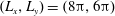
 $L_{x}\times L_{z}=2{\rm\pi}\times {\it\delta}$
.
$L_{x}\times L_{z}=2{\rm\pi}\times {\it\delta}$
.
In figure 5 the root-mean-square (r.m.s.) temperature fluctuation,
 $\langle {\it\phi}^{\prime }{\it\phi}^{\prime }\rangle ^{1/2}$
, is plotted normalised by
$\langle {\it\phi}^{\prime }{\it\phi}^{\prime }\rangle ^{1/2}$
, is plotted normalised by
 $(I_{s}/{\it\delta}q_{N})$
. In the mixed region,
$(I_{s}/{\it\delta}q_{N})$
. In the mixed region,
 $\langle {\it\phi}^{\prime }{\it\phi}^{\prime }\rangle ^{1/2}$
is slightly larger at lower
$\langle {\it\phi}^{\prime }{\it\phi}^{\prime }\rangle ^{1/2}$
is slightly larger at lower
 ${\it\lambda}$
. The larger range of scales apparent in the near-wall region as seen in the flow visualisations in figure 4(c) also indicates this behaviour. In the thermocline, the increase in stability first increases the temperature fluctuations as turbulence is still active and works with an increased mean temperature gradient. At large stability for
${\it\lambda}$
. The larger range of scales apparent in the near-wall region as seen in the flow visualisations in figure 4(c) also indicates this behaviour. In the thermocline, the increase in stability first increases the temperature fluctuations as turbulence is still active and works with an increased mean temperature gradient. At large stability for
 ${\it\lambda}=0.2{-}2.0$
,
${\it\lambda}=0.2{-}2.0$
,
 $\langle {\it\phi}^{\prime }{\it\phi}^{\prime }\rangle ^{1/2}$
decreases near the free surface as turbulence is suppressed.
$\langle {\it\phi}^{\prime }{\it\phi}^{\prime }\rangle ^{1/2}$
decreases near the free surface as turbulence is suppressed.

Figure 5. Temperature fluctuation normalised as
 $\langle {\it\phi}^{\prime }{\it\phi}^{\prime }\rangle ^{1/2}/(I_{s}/{\it\delta}q_{N})$
at
$\langle {\it\phi}^{\prime }{\it\phi}^{\prime }\rangle ^{1/2}/(I_{s}/{\it\delta}q_{N})$
at
 $\mathit{Re}_{{\it\tau}}=395$
,
$\mathit{Re}_{{\it\tau}}=395$
,
 ${\it\alpha}{\it\delta}=8$
(a) and
${\it\alpha}{\it\delta}=8$
(a) and
 $\mathit{Re}_{{\it\tau}}=200{-}800$
,
$\mathit{Re}_{{\it\tau}}=200{-}800$
,
 ${\it\alpha}{\it\delta}=8{-}32$
(b).
${\it\alpha}{\it\delta}=8{-}32$
(b).
This structure contrasts with the numerous recent studies examining inhomogeneous stratified flow in a channel-type configuration (Komori et al.
Reference Komori, Ueda, Ogino and Mizushina1983; Garg et al.
Reference Garg, Ferziger, Monismith and Koseff2000; Armenio & Sarkar Reference Armenio and Sarkar2002; Nieuwstadt Reference Nieuwstadt2005; Taylor, Sarkar & Armenio Reference Taylor, Sarkar and Armenio2005; Wang & Lu Reference Wang and Lu2005; Deusebio et al.
Reference Deusebio, Schlatter, Brethouwer and Lindborg2011; Flores & Riley Reference Flores and Riley2011; Garcia-Villalba & del Alamo Reference Garcia-Villalba and del Alamo2011; Zonta, Onorato & Soldati Reference Zonta, Onorato and Soldati2012) where
 $N$
typically peaks at the walls. Komori et al. (Reference Komori, Ueda, Ogino and Mizushina1983) performed experiments condensing steam in the free surface of an open channel. Garg et al. (Reference Garg, Ferziger, Monismith and Koseff2000) and Wang & Lu (Reference Wang and Lu2005) examined open channel flow with an isothermal surface and an adiabatic or isothermal lower boundary condition while Deusebio et al. (Reference Deusebio, Schlatter, Brethouwer and Lindborg2011) examined the same configuration with constant fixed temperature difference across the channel. The canonical closed channel flow with a fixed temperature difference between the upper and lower walls was examined by Armenio & Sarkar (Reference Armenio and Sarkar2002) and Garcia-Villalba & del Alamo (Reference Garcia-Villalba and del Alamo2011) in statistically steady conditions. These studies can be quantitatively related to our study by converting their
$N$
typically peaks at the walls. Komori et al. (Reference Komori, Ueda, Ogino and Mizushina1983) performed experiments condensing steam in the free surface of an open channel. Garg et al. (Reference Garg, Ferziger, Monismith and Koseff2000) and Wang & Lu (Reference Wang and Lu2005) examined open channel flow with an isothermal surface and an adiabatic or isothermal lower boundary condition while Deusebio et al. (Reference Deusebio, Schlatter, Brethouwer and Lindborg2011) examined the same configuration with constant fixed temperature difference across the channel. The canonical closed channel flow with a fixed temperature difference between the upper and lower walls was examined by Armenio & Sarkar (Reference Armenio and Sarkar2002) and Garcia-Villalba & del Alamo (Reference Garcia-Villalba and del Alamo2011) in statistically steady conditions. These studies can be quantitatively related to our study by converting their
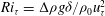 $Ri_{{\it\tau}}={\rm\Delta}{\it\rho}g{\it\delta}/{\it\rho}_{0}u_{{\it\tau}}^{2}$
to
$Ri_{{\it\tau}}={\rm\Delta}{\it\rho}g{\it\delta}/{\it\rho}_{0}u_{{\it\tau}}^{2}$
to
 ${\it\lambda}$
using
${\it\lambda}$
using
 ${\it\lambda}=(Nu/2)Ri_{{\it\tau}}/(PrRe_{{\it\tau}})$
where
${\it\lambda}=(Nu/2)Ri_{{\it\tau}}/(PrRe_{{\it\tau}})$
where
 $Nu$
is the Nusselt number. Garcia-Villalba & del Alamo (Reference Garcia-Villalba and del Alamo2011) cover the range
$Nu$
is the Nusselt number. Garcia-Villalba & del Alamo (Reference Garcia-Villalba and del Alamo2011) cover the range
 ${\it\lambda}=0{-}3.4$
at
${\it\lambda}=0{-}3.4$
at
 $Re_{{\it\tau}}=180{-}550$
and
$Re_{{\it\tau}}=180{-}550$
and
 $Pr=0.7$
(
$Pr=0.7$
(
 $Ri_{b}=0{-}0.462$
), while Armenio & Sarkar (Reference Armenio and Sarkar2002) covered
$Ri_{b}=0{-}0.462$
), while Armenio & Sarkar (Reference Armenio and Sarkar2002) covered
 $Ri_{b}=0{-}0.297$
at
$Ri_{b}=0{-}0.297$
at
 $Re_{{\it\tau}}=180$
,
$Re_{{\it\tau}}=180$
,
 $Pr=0.71$
giving
$Pr=0.71$
giving
 ${\it\lambda}=0{-}2.4$
.
${\it\lambda}=0{-}2.4$
.
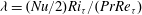
Conditions more related to the present study were examined by Taylor et al. (Reference Taylor, Sarkar and Armenio2005), who used large-eddy simulation (LES) of an open channel flow with a constant heat flux at the upper stress-free boundary and an adiabatic lower wall with periodic spanwise and streamwise boundaries. Our configuration approaches this setting as
 ${\it\alpha}{\it\delta}\rightarrow \infty$
. The results of Taylor et al. (Reference Taylor, Sarkar and Armenio2005) can be compared by converting their
${\it\alpha}{\it\delta}\rightarrow \infty$
. The results of Taylor et al. (Reference Taylor, Sarkar and Armenio2005) can be compared by converting their
 $Ri_{{\it\tau}}$
to
$Ri_{{\it\tau}}$
to
 ${\it\lambda}$
using
${\it\lambda}$
using
 ${\it\lambda}=Ri_{{\it\tau}}/(2PrRe_{{\it\tau}})$
and
${\it\lambda}=Ri_{{\it\tau}}/(2PrRe_{{\it\tau}})$
and
 $E_{r}={\it\lambda}\sqrt{C_{f}/2}$
. They cover the range
$E_{r}={\it\lambda}\sqrt{C_{f}/2}$
. They cover the range
 $Ri_{b}=0{-}0.118$
,
$Ri_{b}=0{-}0.118$
,
 ${\it\lambda}=0{-}0.125$
and
${\it\lambda}=0{-}0.125$
and
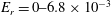 $E_{r}=0{-}6.8\times 10^{-3}$
at
$E_{r}=0{-}6.8\times 10^{-3}$
at
 $Re_{{\it\tau}}=400$
and
$Re_{{\it\tau}}=400$
and
 $Pr=5$
, indicating that stratification is relatively weak.
$Pr=5$
, indicating that stratification is relatively weak.

Figure 6. Variation of instantaneous bulk flow properties over non-dimensional flow time at
 $\mathit{Re}_{{\it\tau}}=395$
,
$\mathit{Re}_{{\it\tau}}=395$
,
 ${\it\alpha}{\it\delta}=8$
: (a) skin friction
${\it\alpha}{\it\delta}=8$
: (a) skin friction
 $C_{f}=2\langle u_{{\it\tau}}/u_{b}\rangle ^{2}$
and (b) instantaneous plane-averaged temperature difference
$C_{f}=2\langle u_{{\it\tau}}/u_{b}\rangle ^{2}$
and (b) instantaneous plane-averaged temperature difference
 ${\rm\Delta}{\it\phi}/\langle {\rm\Delta}{\it\phi}\rangle +A$
where
${\rm\Delta}{\it\phi}/\langle {\rm\Delta}{\it\phi}\rangle +A$
where
 $A$
is a vertical offset given in the figure.
$A$
is a vertical offset given in the figure.
There are also numerous studies of the atmospheric surface layer under stable conditions (e.g. Nieuwstadt Reference Nieuwstadt1984, Reference Nieuwstadt2005; Grachev et al.
Reference Grachev, Fairall, Persson, Andreas and Guest2005; Wiel et al.
Reference Wiel, Moene, Ronde and Jonker2008; Sorbjan & Grachev Reference Sorbjan and Grachev2010; Flores & Riley Reference Flores and Riley2011; Grachev et al.
Reference Grachev, Andreas, Fairall, Guest and Persson2013). Unlike the stable atmospheric boundary layer, where
 $\langle b^{\prime }w^{\prime }\rangle$
and
$\langle b^{\prime }w^{\prime }\rangle$
and
 $\langle u^{\prime }w^{\prime }\rangle$
both decrease with height, in the present open channel configuration
$\langle u^{\prime }w^{\prime }\rangle$
both decrease with height, in the present open channel configuration
 $\langle b^{\prime }w^{\prime }\rangle$
is zero at the wall and increases over most of the channel height and is non-monotonic. The inner wall region is then expected to be less susceptible to the transient re-laminarisation events that may be seen in these flows at low Reynolds number and high
$\langle b^{\prime }w^{\prime }\rangle$
is zero at the wall and increases over most of the channel height and is non-monotonic. The inner wall region is then expected to be less susceptible to the transient re-laminarisation events that may be seen in these flows at low Reynolds number and high
 ${\it\lambda}$
.
${\it\lambda}$
.
A consequence of our configuration is that we are able to attain statistically steady flow at relatively minimal domain sizes with regions of strong stratification present in the flow. The time-varying plane-averaged skin friction coefficient
 $C_{f}=2\langle u_{{\it\tau}}/u_{b}\rangle ^{2}$
, is given in figure 6(a) for our
$C_{f}=2\langle u_{{\it\tau}}/u_{b}\rangle ^{2}$
, is given in figure 6(a) for our
 ${\it\lambda}=0.1,0.5,1.0$
simulations. The time variation in the plane-averaged
${\it\lambda}=0.1,0.5,1.0$
simulations. The time variation in the plane-averaged
 ${\rm\Delta}{\it\phi}$
normalised by time-averaged
${\rm\Delta}{\it\phi}$
normalised by time-averaged
 $\langle {\rm\Delta}{\it\phi}\rangle$
is illustrated in figure 6(b) for
$\langle {\rm\Delta}{\it\phi}\rangle$
is illustrated in figure 6(b) for
 ${\it\lambda}=0{-}2.0$
. In both the time trace of
${\it\lambda}=0{-}2.0$
. In both the time trace of
 $C_{f}$
and
$C_{f}$
and
 ${\rm\Delta}{\it\phi}$
there is a range of long-time-scale oscillations of period
${\rm\Delta}{\it\phi}$
there is a range of long-time-scale oscillations of period
 ${\rm\Delta}t\simeq 5{-}10$
, longer than the turnover time
${\rm\Delta}t\simeq 5{-}10$
, longer than the turnover time
 $t=1$
and the Brunt–Väisälä period
$t=1$
and the Brunt–Väisälä period
 $u_{{\it\tau}}/N{\it\delta}\lesssim 2$
for
$u_{{\it\tau}}/N{\it\delta}\lesssim 2$
for
 ${\it\lambda}=0.05$
. Similar observations were seen the closed channel flow of Garcia-Villalba & del Alamo (Reference Garcia-Villalba and del Alamo2011). In all cases here, however, the results converge to a statistically steady fully developed flow. The Reynolds number based on friction velocity computed directly from the flow field,
${\it\lambda}=0.05$
. Similar observations were seen the closed channel flow of Garcia-Villalba & del Alamo (Reference Garcia-Villalba and del Alamo2011). In all cases here, however, the results converge to a statistically steady fully developed flow. The Reynolds number based on friction velocity computed directly from the flow field,
 $u_{{\it\tau}}^{\ast }$
, is displayed in table 1 as
$u_{{\it\tau}}^{\ast }$
, is displayed in table 1 as
 $Re_{{\it\tau}}^{\ast }$
. In all cases the result is within 0.1 % of the nominal
$Re_{{\it\tau}}^{\ast }$
. In all cases the result is within 0.1 % of the nominal
 $Re_{{\it\tau}}$
. This is in contrast to the stratified wall flow of Garcia-Villalba & del Alamo (Reference Garcia-Villalba and del Alamo2011) who found that much larger domain sizes were required in order to attain well-behaved statistically steady flow. The behaviour they observed was related to re-laminarisation at the wall and had a Reynolds number and
$Re_{{\it\tau}}$
. This is in contrast to the stratified wall flow of Garcia-Villalba & del Alamo (Reference Garcia-Villalba and del Alamo2011) who found that much larger domain sizes were required in order to attain well-behaved statistically steady flow. The behaviour they observed was related to re-laminarisation at the wall and had a Reynolds number and
 ${\it\lambda}$
dependence, so at
${\it\lambda}$
dependence, so at
 ${\it\lambda}=3.4$
and
${\it\lambda}=3.4$
and
 $Re_{{\it\tau}}=550$
,
$Re_{{\it\tau}}=550$
,
 $(L_{x},L_{y})=(8{\rm\pi},6{\rm\pi})$
was required. The present results at
$(L_{x},L_{y})=(8{\rm\pi},6{\rm\pi})$
was required. The present results at
 $Re_{{\it\tau}}=395$
show no signs of re-laminarisation at the wall or divergence of the flow statistics in time with
$Re_{{\it\tau}}=395$
show no signs of re-laminarisation at the wall or divergence of the flow statistics in time with
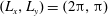 $(L_{x},L_{y})=(2{\rm\pi},{\rm\pi})$
up to our most stable case
$(L_{x},L_{y})=(2{\rm\pi},{\rm\pi})$
up to our most stable case
 ${\it\lambda}=2.0$
.
${\it\lambda}=2.0$
.
In our
 $Re=200$
tests we adopt initially a
$Re=200$
tests we adopt initially a
 $(L_{x},L_{y})=(4{\rm\pi},2{\rm\pi})$
domain to maintain the same size
$(L_{x},L_{y})=(4{\rm\pi},2{\rm\pi})$
domain to maintain the same size
 $(L_{x}^{+},L_{y}^{+})$
in wall units. For
$(L_{x}^{+},L_{y}^{+})$
in wall units. For
 ${\it\lambda}=1.0$
at
${\it\lambda}=1.0$
at
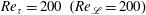 $Re_{{\it\tau}}=200~(Re_{\mathscr{L}}=200)$
, the flow had laminar streaks at the wall spanning the length of the domain and statistically steady conditions were not obtained. The domain size was increased to
$Re_{{\it\tau}}=200~(Re_{\mathscr{L}}=200)$
, the flow had laminar streaks at the wall spanning the length of the domain and statistically steady conditions were not obtained. The domain size was increased to
 $(8{\rm\pi},4{\rm\pi})$
and the flow remained turbulent across the entire wall region and a statistically steady fully developed solution was obtained. At
$(8{\rm\pi},4{\rm\pi})$
and the flow remained turbulent across the entire wall region and a statistically steady fully developed solution was obtained. At
 ${\it\lambda}=0.5$
at
${\it\lambda}=0.5$
at
 $Re_{{\it\tau}}=200$
the laminar streaks or patches were not observed at
$Re_{{\it\tau}}=200$
the laminar streaks or patches were not observed at
 $(4{\rm\pi},2{\rm\pi})$
.
$(4{\rm\pi},2{\rm\pi})$
.
With increasing stability
 ${\it\lambda}$
, the skin friction coefficient, shown in table 1, decreases as the flow accelerates to a higher mean bulk velocity. The profile of the mean streamwise velocity is given in figure 7(a,b) with vertical location in wall units
${\it\lambda}$
, the skin friction coefficient, shown in table 1, decreases as the flow accelerates to a higher mean bulk velocity. The profile of the mean streamwise velocity is given in figure 7(a,b) with vertical location in wall units
 $z^{+}=zu_{{\it\tau}}/{\it\nu}$
. The velocity profiles illustrate that the inner boundary layer,
$z^{+}=zu_{{\it\tau}}/{\it\nu}$
. The velocity profiles illustrate that the inner boundary layer,
 $z^{+}<40$
, is relatively unaffected, even at
$z^{+}<40$
, is relatively unaffected, even at
 ${\it\lambda}=2.0$
where there is approximately a factor of two increase in free-surface velocity compared with neutral flow. A clear separation of the velocity profiles only appears for
${\it\lambda}=2.0$
where there is approximately a factor of two increase in free-surface velocity compared with neutral flow. A clear separation of the velocity profiles only appears for
 $z^{+}>100$
. This contrasts with the stratified wall flows of Armenio & Sarkar (Reference Armenio and Sarkar2002); Garcia-Villalba & del Alamo (Reference Garcia-Villalba and del Alamo2011) where differences were clearly apparent in velocity and shear-stress profiles at
$z^{+}>100$
. This contrasts with the stratified wall flows of Armenio & Sarkar (Reference Armenio and Sarkar2002); Garcia-Villalba & del Alamo (Reference Garcia-Villalba and del Alamo2011) where differences were clearly apparent in velocity and shear-stress profiles at
 ${\it\lambda}=2$
,
${\it\lambda}=2$
,
 $Re_{{\it\tau}}=550$
(Garcia-Villalba & del Alamo Reference Garcia-Villalba and del Alamo2011) and
$Re_{{\it\tau}}=550$
(Garcia-Villalba & del Alamo Reference Garcia-Villalba and del Alamo2011) and
 ${\it\lambda}=1$
,
${\it\lambda}=1$
,
 $Re_{{\it\tau}}=180$
(Armenio & Sarkar Reference Armenio and Sarkar2002) at
$Re_{{\it\tau}}=180$
(Armenio & Sarkar Reference Armenio and Sarkar2002) at
 $z=0.1$
. In our
$z=0.1$
. In our
 $Re_{{\it\tau}}=800$
result, the velocity profile lies close to the
$Re_{{\it\tau}}=800$
result, the velocity profile lies close to the
 ${\it\lambda}=0.1$
,
${\it\lambda}=0.1$
,
 $Re_{{\it\tau}}=395$
curve until
$Re_{{\it\tau}}=395$
curve until
 $z^{+}\simeq 350$
, well into the outer layer. The influence of
$z^{+}\simeq 350$
, well into the outer layer. The influence of
 ${\it\alpha}{\it\delta}$
on the mean velocity profile appears to be relatively weak. In figure 7(b) the flow at
${\it\alpha}{\it\delta}$
on the mean velocity profile appears to be relatively weak. In figure 7(b) the flow at
 ${\it\lambda}=0.5$
,
${\it\lambda}=0.5$
,
 ${\it\alpha}{\it\delta}=32$
is nearly indistinguishable from the curve at
${\it\alpha}{\it\delta}=32$
is nearly indistinguishable from the curve at
 ${\it\alpha}{\it\delta}=8$
. In figure 8(a,b), the shear stress
${\it\alpha}{\it\delta}=8$
. In figure 8(a,b), the shear stress
 $\langle u^{\prime }w^{\prime }\rangle$
is given for the same flows. As suggested by the velocity profiles, there is only slight variation from the neutral case over
$\langle u^{\prime }w^{\prime }\rangle$
is given for the same flows. As suggested by the velocity profiles, there is only slight variation from the neutral case over
 $z=0{-}0.3$
, while at
$z=0{-}0.3$
, while at
 ${\it\lambda}=0.5{-}2.0$
the turbulent shear stress is significantly damped for
${\it\lambda}=0.5{-}2.0$
the turbulent shear stress is significantly damped for
 $z>0.6$
and at
$z>0.6$
and at
 ${\it\lambda}=2.0~\langle u^{\prime }w^{\prime }\rangle \simeq 0$
for
${\it\lambda}=2.0~\langle u^{\prime }w^{\prime }\rangle \simeq 0$
for
 $z>0.9$
.
$z>0.9$
.

Figure 7. Variation of mean streamwise velocity profile
 $u$
with height in wall units: (a) for
$u$
with height in wall units: (a) for
 $Re_{{\it\tau}}=395$
,
$Re_{{\it\tau}}=395$
,
 ${\it\alpha}{\it\delta}=8$
and
${\it\alpha}{\it\delta}=8$
and
 ${\it\lambda}=0{-}2.0$
; and (b)
${\it\lambda}=0{-}2.0$
; and (b)
 ${\it\alpha}{\it\delta}=8{-}32$
.
${\it\alpha}{\it\delta}=8{-}32$
.

Figure 8. Turbulent shear stress,
 $-\langle u^{\prime }w^{\prime }\rangle$
at
$-\langle u^{\prime }w^{\prime }\rangle$
at
 $\mathit{Re}_{{\it\tau}}=395$
,
$\mathit{Re}_{{\it\tau}}=395$
,
 ${\it\alpha}{\it\delta}=8$
(a) and
${\it\alpha}{\it\delta}=8$
(a) and
 $\mathit{Re}_{{\it\tau}}=200{-}800$
,
$\mathit{Re}_{{\it\tau}}=200{-}800$
,
 ${\it\alpha}{\it\delta}=8{-}32$
(b).
${\it\alpha}{\it\delta}=8{-}32$
(b).
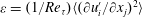
In the statistically steady flow considered here the non-dimensional time-averaged temperature transport equation is
 $$\begin{eqnarray}0=-\frac{\text{d}\langle w^{\prime }{\it\phi}^{\prime }\rangle }{\text{d}z}+\frac{1}{Re_{{\it\tau}}Pr}\frac{\text{d}^{2}\langle {\it\phi}\rangle }{\text{d}z^{2}}+qe.\end{eqnarray}$$
In the laminar limit, it is expected that
 $\partial {\it\phi}/\partial z\sim PrRe_{{\it\tau}}I_{s}/{\it\delta}q_{N}$
. These conditions are approached near the free surface at high
$\partial {\it\phi}/\partial z\sim PrRe_{{\it\tau}}I_{s}/{\it\delta}q_{N}$
. These conditions are approached near the free surface at high
 ${\it\lambda}$
, resulting in the increase in surface temperature at
${\it\lambda}$
, resulting in the increase in surface temperature at
 ${\it\lambda}=0.5$
over
${\it\lambda}=0.5$
over
 $Re_{{\it\tau}}=200{-}800$
. In the limit of
$Re_{{\it\tau}}=200{-}800$
. In the limit of
 $1/Re_{{\it\tau}}Pr\rightarrow 0$
we can integrate over the channel height with the boundary condition
$1/Re_{{\it\tau}}Pr\rightarrow 0$
we can integrate over the channel height with the boundary condition
 $\langle {\it\phi}^{\prime }w^{\prime }\rangle =0$
at
$\langle {\it\phi}^{\prime }w^{\prime }\rangle =0$
at
 $z=0$
to obtain
$z=0$
to obtain
 $$\begin{eqnarray}-\langle {\it\phi}^{\prime }w^{\prime }\rangle /(I_{s}/{\it\delta}q_{N})=\left(z-\text{e}^{(z-1){\it\alpha}{\it\delta}}\right).\end{eqnarray}$$
Plotting this limit for
 ${\it\alpha}{\it\delta}=8{-}32$
together with profiles of
${\it\alpha}{\it\delta}=8{-}32$
together with profiles of
 $-\langle {\it\phi}^{\prime }w^{\prime }\rangle$
in figure 9(a,b) reveals the extent to which the increased stability has reduced the turbulent heat flux. Over the mixed region the profiles
$-\langle {\it\phi}^{\prime }w^{\prime }\rangle$
in figure 9(a,b) reveals the extent to which the increased stability has reduced the turbulent heat flux. Over the mixed region the profiles
 $-\langle {\it\phi}^{\prime }w^{\prime }\rangle$
differ only slightly from (3.2), while through the thermocline the scalar flux is increasingly damped as suggested by the temperature profiles. Adjacent to the surface at
$-\langle {\it\phi}^{\prime }w^{\prime }\rangle$
differ only slightly from (3.2), while through the thermocline the scalar flux is increasingly damped as suggested by the temperature profiles. Adjacent to the surface at
 ${\it\lambda}=0.5{-}2$
a region exists where
${\it\lambda}=0.5{-}2$
a region exists where
 $-\langle {\it\phi}^{\prime }w^{\prime }\rangle <0$
indicating counter-gradient heat transfer, as has been reported elsewhere in strongly stratified conditions (see Komori et al.
Reference Komori, Ueda, Ogino and Mizushina1983; Gerz, Schumann & Elghobashi Reference Gerz, Schumann and Elghobashi1989; Holt et al.
Reference Holt, Koseff and Ferziger1992; Taylor et al.
Reference Taylor, Sarkar and Armenio2005).
$-\langle {\it\phi}^{\prime }w^{\prime }\rangle <0$
indicating counter-gradient heat transfer, as has been reported elsewhere in strongly stratified conditions (see Komori et al.
Reference Komori, Ueda, Ogino and Mizushina1983; Gerz, Schumann & Elghobashi Reference Gerz, Schumann and Elghobashi1989; Holt et al.
Reference Holt, Koseff and Ferziger1992; Taylor et al.
Reference Taylor, Sarkar and Armenio2005).

Figure 9. Scalar flux normalised as
 $-\langle {\it\phi}^{\prime }w^{\prime }\rangle /(I_{s}/{\it\delta}q_{N})$
at
$-\langle {\it\phi}^{\prime }w^{\prime }\rangle /(I_{s}/{\it\delta}q_{N})$
at
 $\mathit{Re}_{{\it\tau}}=395$
,
$\mathit{Re}_{{\it\tau}}=395$
,
 ${\it\alpha}{\it\delta}=8$
(a) and
${\it\alpha}{\it\delta}=8$
(a) and
 $\mathit{Re}_{{\it\tau}}=395{-}800$
,
$\mathit{Re}_{{\it\tau}}=395{-}800$
,
 ${\it\alpha}{\it\delta}=8{-}32$
(b).
${\it\alpha}{\it\delta}=8{-}32$
(b).
It is clear that there is rapid variation in flow stability with
 $z$
, allowing the influence of stratification to be examined within a single simulation flow field.
$z$
, allowing the influence of stratification to be examined within a single simulation flow field.
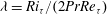
4. Transition to local energetic equilibrium and turbulence suppression
4.1. Criterion for onset of strong stratification
With the flow being statistically stationary and with homogeneity in the
 $x{-}y$
plane, the TKE transport equations can be written in non-dimensional form as
$x{-}y$
plane, the TKE transport equations can be written in non-dimensional form as
 $$\begin{eqnarray}\frac{\text{d}}{\text{d}z}\langle w^{\prime }k\rangle +\frac{\text{d}}{\text{d}z}\langle w^{\prime }p^{\prime }\rangle -\frac{1}{Re_{{\it\tau}}}\frac{\text{d}^{2}k}{\text{d}z^{2}}=P-{\it\varepsilon}-B,\end{eqnarray}$$
where the TKE is
 $k=0.5\langle u_{i}^{\prime }u_{i}^{\prime }\rangle$
, the buoyancy flux
$k=0.5\langle u_{i}^{\prime }u_{i}^{\prime }\rangle$
, the buoyancy flux
 $B=-{\it\lambda}\langle {\it\phi}^{\prime }w^{\prime }\rangle$
, the turbulence dissipation rate
$B=-{\it\lambda}\langle {\it\phi}^{\prime }w^{\prime }\rangle$
, the turbulence dissipation rate
 ${\it\varepsilon}=(1/Re_{{\it\tau}})\langle (\partial u_{i}^{\prime }/\partial x_{j})^{2}\rangle$
and the turbulence production term
${\it\varepsilon}=(1/Re_{{\it\tau}})\langle (\partial u_{i}^{\prime }/\partial x_{j})^{2}\rangle$
and the turbulence production term
 $P=-\langle u^{\prime }w^{\prime }\rangle \mathscr{S}$
where
$P=-\langle u^{\prime }w^{\prime }\rangle \mathscr{S}$
where
 $\mathscr{S}=\text{d}\langle u\rangle /\text{d}z$
. The transport terms on the left-hand side of (4.1) are the turbulent convection (
$\mathscr{S}=\text{d}\langle u\rangle /\text{d}z$
. The transport terms on the left-hand side of (4.1) are the turbulent convection (
 $T$
), pressure transport and viscous diffusion terms respectively. When the terms on the left-hand side are zero, the flow is in local equilibrium, with production and dissipation in balance,
$T$
), pressure transport and viscous diffusion terms respectively. When the terms on the left-hand side are zero, the flow is in local equilibrium, with production and dissipation in balance,
 $P-{\it\varepsilon}-B=0$
. The ratio of the dominant terms
$P-{\it\varepsilon}-B=0$
. The ratio of the dominant terms
 $P$
,
$P$
,
 $B$
and
$B$
and
 $T$
to the total dissipation
$T$
to the total dissipation
 ${\it\varepsilon}+B$
, are shown over the channel depth in figure 10.
${\it\varepsilon}+B$
, are shown over the channel depth in figure 10.

Figure 10. Turbulence kinetic energy transport terms as a ratio of total dissipation: (a) production
 $P/({\it\varepsilon}+B)$
, (b) turbulent diffusion
$P/({\it\varepsilon}+B)$
, (b) turbulent diffusion
 $T/({\it\varepsilon}+B)$
and (c) buoyancy flux
$T/({\it\varepsilon}+B)$
and (c) buoyancy flux
 $-B/({\it\varepsilon}+B)$
or equivalently
$-B/({\it\varepsilon}+B)$
or equivalently
 $-R_{f}$
.
$-R_{f}$
.
At
 ${\it\lambda}=0$
a region of quasi-equilibrium where
${\it\lambda}=0$
a region of quasi-equilibrium where
 $P\simeq {\it\varepsilon}$
exists over
$P\simeq {\it\varepsilon}$
exists over
 $(50\lesssim z^{+}\lesssim 0.5Re_{{\it\tau}})$
. Above this region, the turbulent convection term increases and the outer layer is a net sink of turbulence. This compares well with experimental observation in neutral conditions in open channel flow (Komori et al.
Reference Komori, Ueda, Ogino and Mizushina1983; Nezu & Rodi Reference Nezu and Rodi1986) and DNS of closed channel flow (Moser et al.
Reference Moser, Kim and Mansour1999) over
$(50\lesssim z^{+}\lesssim 0.5Re_{{\it\tau}})$
. Above this region, the turbulent convection term increases and the outer layer is a net sink of turbulence. This compares well with experimental observation in neutral conditions in open channel flow (Komori et al.
Reference Komori, Ueda, Ogino and Mizushina1983; Nezu & Rodi Reference Nezu and Rodi1986) and DNS of closed channel flow (Moser et al.
Reference Moser, Kim and Mansour1999) over
 $Re_{{\it\tau}}=395{-}640$
. With increasing
$Re_{{\it\tau}}=395{-}640$
. With increasing
 ${\it\lambda}$
the equilibrium region, as indicated by
${\it\lambda}$
the equilibrium region, as indicated by
 $P/({\it\varepsilon}+B)\sim 1$
, extends further towards the free surface. At
$P/({\it\varepsilon}+B)\sim 1$
, extends further towards the free surface. At
 ${\it\lambda}=0.5{-}1.0$
, this equilibrium region extends to a near-surface region at
${\it\lambda}=0.5{-}1.0$
, this equilibrium region extends to a near-surface region at
 $z\simeq 0.8$
above which there is a separate behaviour that we return to in § 6. Normalised in this form, the buoyancy flux is also known as the generalised flux Richardson number (Ivey & Imberger Reference Ivey and Imberger1991),
$z\simeq 0.8$
above which there is a separate behaviour that we return to in § 6. Normalised in this form, the buoyancy flux is also known as the generalised flux Richardson number (Ivey & Imberger Reference Ivey and Imberger1991),
 $$\begin{eqnarray}R_{f}=\frac{B}{B+{\it\varepsilon}},\end{eqnarray}$$
which has observed limit values of
 $R_{f,c}\simeq 0.17{-}0.25$
(Ellison Reference Ellison1957; Osborn Reference Osborn1980; Ivey et al.
Reference Ivey, Winters and Koseff2008; Garcia-Villalba & del Alamo Reference Garcia-Villalba and del Alamo2011). With increasing stability,
$R_{f,c}\simeq 0.17{-}0.25$
(Ellison Reference Ellison1957; Osborn Reference Osborn1980; Ivey et al.
Reference Ivey, Winters and Koseff2008; Garcia-Villalba & del Alamo Reference Garcia-Villalba and del Alamo2011). With increasing stability,
 $R_{f}$
(figure 10
c) rises to peak values in the region
$R_{f}$
(figure 10
c) rises to peak values in the region
 $z=0.75{-}0.85$
where the scalar flux profile decreases rapidly with
$z=0.75{-}0.85$
where the scalar flux profile decreases rapidly with
 $z$
(figure 9). At
$z$
(figure 9). At
 ${\it\lambda}=2.0$
over
${\it\lambda}=2.0$
over
 $z=0.5{-}0.7$
the flow approaches a local energetic mixing limit
$z=0.5{-}0.7$
the flow approaches a local energetic mixing limit
 $R_{f,c}\simeq 0.18$
.
$R_{f,c}\simeq 0.18$
.
This transition can also be seen in the length scales
 $l_{C}$
and
$l_{C}$
and
 $l_{O}$
which are shown in figure 11 with
$l_{O}$
which are shown in figure 11 with
 $z$
together with the length scale
$z$
together with the length scale
 ${\it\eta}$
. With increasing buoyancy,
${\it\eta}$
. With increasing buoyancy,
 $l_{C}$
and
$l_{C}$
and
 $l_{O}$
reduce, while
$l_{O}$
reduce, while
 ${\it\eta}$
is relatively unaffected. The variation of the ratio of the outer length scales
${\it\eta}$
is relatively unaffected. The variation of the ratio of the outer length scales
 $Ri=(l_{C}/l_{O})^{4/3}$
with
$Ri=(l_{C}/l_{O})^{4/3}$
with
 $z$
is shown in figure 12. In the near-wall region
$z$
is shown in figure 12. In the near-wall region
 $Ri$
rises from near-neutral values with height and with increasing flow stability. At
$Ri$
rises from near-neutral values with height and with increasing flow stability. At
 ${\it\lambda}=1.0$
between
${\it\lambda}=1.0$
between
 $z=0.6{-}0.77$
,
$z=0.6{-}0.77$
,
 $Ri$
appears to asymptote to
$Ri$
appears to asymptote to
 $Ri_{c}=0.2$
before rising above this limit at
$Ri_{c}=0.2$
before rising above this limit at
 $z=0.77$
. At
$z=0.77$
. At
 ${\it\lambda}=2.0$
the asymptote occurs over
${\it\lambda}=2.0$
the asymptote occurs over
 $z=0.5{-}0.77$
. The onset of limit conditions is similar to that observed for
$z=0.5{-}0.77$
. The onset of limit conditions is similar to that observed for
 $R_{f}$
. The relationship between the two parameters can be formed in equilibrium conditions from definitions as
$R_{f}$
. The relationship between the two parameters can be formed in equilibrium conditions from definitions as
 $Pr_{t}=Ri/R_{f}$
where the turbulent Prandtl number is
$Pr_{t}=Ri/R_{f}$
where the turbulent Prandtl number is
 $$\begin{eqnarray}Pr_{t}=\frac{-\langle u^{\prime }w^{\prime }\rangle /\mathscr{S}}{B/\mathscr{N}^{2}}\end{eqnarray}$$
and
 $\mathscr{N}^{2}={\it\lambda}\text{d}\langle {\it\phi}\rangle /\text{d}z$
is the non-dimensional Brunt–Väisälä frequency. The profiles of
$\mathscr{N}^{2}={\it\lambda}\text{d}\langle {\it\phi}\rangle /\text{d}z$
is the non-dimensional Brunt–Väisälä frequency. The profiles of
 $Pr_{t}$
in figure 13 show that, over the region
$Pr_{t}$
in figure 13 show that, over the region
 $z<0.6$
, with increasing stability the flow increases from
$z<0.6$
, with increasing stability the flow increases from
 $Pr_{t}\simeq 0.8$
in neutral conditions to a nearly constant value of
$Pr_{t}\simeq 0.8$
in neutral conditions to a nearly constant value of
 $Pr_{t}=1.0$
at
$Pr_{t}=1.0$
at
 ${\it\lambda}=2.0$
.
${\it\lambda}=2.0$
.

Figure 11. Variation of length scales
 $l_{O},l_{C},{\it\eta}$
normalised by
$l_{O},l_{C},{\it\eta}$
normalised by
 ${\it\delta}$
with
${\it\delta}$
with
 $z$
for (a)
$z$
for (a)
 ${\it\lambda}=0{-}2.0$
at
${\it\lambda}=0{-}2.0$
at
 $Re_{{\it\tau}}=395$
with lines defined in figure 10; (b)
$Re_{{\it\tau}}=395$
with lines defined in figure 10; (b)
 $Re_{{\it\tau}}=200{-}800$
and
$Re_{{\it\tau}}=200{-}800$
and
 ${\it\lambda}=0.5{-}1.0$
.
${\it\lambda}=0.5{-}1.0$
.

Figure 12. Variation of
 $Ri$
with
$Ri$
with
 $z$
for (a)
$z$
for (a)
 $Re_{{\it\tau}}=395$
with
$Re_{{\it\tau}}=395$
with
 ${\it\lambda}=0.05{-}1.0$
and (b)
${\it\lambda}=0.05{-}1.0$
and (b)
 $\mathit{Re}_{{\it\tau}}=200{-}800$
,
$\mathit{Re}_{{\it\tau}}=200{-}800$
,
 ${\it\alpha}{\it\delta}=8{-}32$
and
${\it\alpha}{\it\delta}=8{-}32$
and
 ${\it\lambda}=0.5{-}1.0$
.
${\it\lambda}=0.5{-}1.0$
.

Figure 13.
 $Pr_{t}$
for
$Pr_{t}$
for
 ${\it\lambda}=0{-}2.0$
.
${\it\lambda}=0{-}2.0$
.
It is clear that
 ${\it\lambda}\simeq 1$
represents a transition to local limit conditions for this flow in terms of
${\it\lambda}\simeq 1$
represents a transition to local limit conditions for this flow in terms of
 $Pr_{t}\rightarrow 1$
and
$Pr_{t}\rightarrow 1$
and
 $P/({\it\varepsilon}+B)\sim 1$
and that
$P/({\it\varepsilon}+B)\sim 1$
and that
 $Ri\rightarrow Ri_{c}$
,
$Ri\rightarrow Ri_{c}$
,
 $R_{f}\rightarrow R_{f,c}$
over an increasing portion of the boundary layer height with
$R_{f}\rightarrow R_{f,c}$
over an increasing portion of the boundary layer height with
 ${\it\lambda}>1$
.
${\it\lambda}>1$
.
4.2.
 $\mathscr{R}$
affected regime
$\mathscr{R}$
affected regime

With increasing stratification,
 $l_{O}$
approaches the smallest scales of turbulent motion
$l_{O}$
approaches the smallest scales of turbulent motion
 ${\it\eta}$
. The ratio
${\it\eta}$
. The ratio
 $\mathscr{R}=(l_{O}/{\it\eta})^{4/3}$
is plotted in figure 14. The parameter varies over four orders of magnitude across the channel height. In the wall region
$\mathscr{R}=(l_{O}/{\it\eta})^{4/3}$
is plotted in figure 14. The parameter varies over four orders of magnitude across the channel height. In the wall region
 $l_{O}\gg {\it\eta}$
, indicating a wide separation between smallest scales and buoyancy affected scales, while with increasing
$l_{O}\gg {\it\eta}$
, indicating a wide separation between smallest scales and buoyancy affected scales, while with increasing
 $z$
and
$z$
and
 ${\it\lambda}$
this separation is reduced.
${\it\lambda}$
this separation is reduced.

Figure 14. Variation of
 $\mathscr{R}$
with
$\mathscr{R}$
with
 $z$
at
$z$
at
 $\mathit{Re}_{{\it\tau}}=395$
(a) and
$\mathit{Re}_{{\it\tau}}=395$
(a) and
 $\mathit{Re}_{{\it\tau}}=200{-}800$
(b). In (a) the thin solid line indicates
$\mathit{Re}_{{\it\tau}}=200{-}800$
(b). In (a) the thin solid line indicates
 $\mathscr{R}=Re_{{\it\Lambda}}$
estimated from
$\mathscr{R}=Re_{{\it\Lambda}}$
estimated from
 $Re_{{\it\Lambda}}=(1-z)^{2}Re_{{\it\tau}}/{\it\lambda}(z-\text{e}^{(z-1){\it\alpha}{\it\delta}})$
at
$Re_{{\it\Lambda}}=(1-z)^{2}Re_{{\it\tau}}/{\it\lambda}(z-\text{e}^{(z-1){\it\alpha}{\it\delta}})$
at
 $Re_{{\it\tau}}=395$
and
$Re_{{\it\tau}}=395$
and
 ${\it\lambda}=0.5$
. Solid horizontal line indicates
${\it\lambda}=0.5$
. Solid horizontal line indicates
 $\mathscr{R}=7$
.
$\mathscr{R}=7$
.
Recent discussion has identified this reduced separation of scales with the transition to a viscous regime of behaviour (Lindborg Reference Lindborg2006; Brethouwer et al.
Reference Brethouwer, Billant, Lindborg and Chomaz2007; Flores & Riley Reference Flores and Riley2011; Chung & Matheou Reference Chung and Matheou2012). Shih et al. (Reference Shih, Koseff, Ivey and Ferziger2005) examined the mixing characteristics in homogeneous stratified shear flow and found that
 $\mathscr{R}_{c}\lesssim 7$
indicated transition to a molecular diffusive mixing regime. In a similar flow Brethouwer et al. (Reference Brethouwer, Billant, Lindborg and Chomaz2007) showed that
$\mathscr{R}_{c}\lesssim 7$
indicated transition to a molecular diffusive mixing regime. In a similar flow Brethouwer et al. (Reference Brethouwer, Billant, Lindborg and Chomaz2007) showed that
 $\mathscr{R}_{c}=1$
indicates the transition from a classic Kolmogorov energy cascade to a regime where vertical viscous shearing is important.
$\mathscr{R}_{c}=1$
indicates the transition from a classic Kolmogorov energy cascade to a regime where vertical viscous shearing is important.
Applying these limits here suggests the low-
 $\mathscr{R}$
regime is attained over a part of the domain height for
$\mathscr{R}$
regime is attained over a part of the domain height for
 ${\it\lambda}\gtrsim 0.5$
at
${\it\lambda}\gtrsim 0.5$
at
 $Re_{{\it\tau}}=395$
. The limit
$Re_{{\it\tau}}=395$
. The limit
 $\mathscr{R}_{c}=7$
intersects with the
$\mathscr{R}_{c}=7$
intersects with the
 $\mathscr{R}$
profiles in figure 14(a) at
$\mathscr{R}$
profiles in figure 14(a) at
 $z=0.9$
, 0.8 and 0.7 for
$z=0.9$
, 0.8 and 0.7 for
 ${\it\lambda}=0.5$
, 1.0 and 2.0 respectively for
${\it\lambda}=0.5$
, 1.0 and 2.0 respectively for
 $Re_{{\it\tau}}=395$
. The onset of a more suppressed regime of turbulent flow is also apparent in our mean flow statistics. In figure 10(a) the turbulence production term at
$Re_{{\it\tau}}=395$
. The onset of a more suppressed regime of turbulent flow is also apparent in our mean flow statistics. In figure 10(a) the turbulence production term at
 ${\it\lambda}=2$
falls below the
${\it\lambda}=2$
falls below the
 ${\it\lambda}=1$
curve at
${\it\lambda}=1$
curve at
 $z\simeq 0.8$
while the
$z\simeq 0.8$
while the
 ${\it\lambda}=1$
curve falls below the
${\it\lambda}=1$
curve falls below the
 ${\it\lambda}=0.5$
curve at
${\it\lambda}=0.5$
curve at
 $z\simeq 0.9$
. In figures 8 and 9 the shear stress and buoyancy flux are also reduced in these regions as are the buoyancy fluctuations in figure 5. The normal stresses are plotted in figures 15–17. In the neutral case our results are comparable with available data for open channel flow over
$z\simeq 0.9$
. In figures 8 and 9 the shear stress and buoyancy flux are also reduced in these regions as are the buoyancy fluctuations in figure 5. The normal stresses are plotted in figures 15–17. In the neutral case our results are comparable with available data for open channel flow over
 $Re_{{\it\tau}}=134{-}1280$
(Handler et al.
Reference Handler, Swean, Leighton and Swearingen1993; Komori et al.
Reference Komori, Nagaosa, Murakami, Chiba, Ishii and Kuwahara1993; Handler et al.
Reference Handler, Saylor, Leighton and Rovelstad1999; Calmet & Magnaudet Reference Calmet and Magnaudet2003; Nagaosa & Handler Reference Nagaosa and Handler2003). In stratified conditions, the wall-normal stress
$Re_{{\it\tau}}=134{-}1280$
(Handler et al.
Reference Handler, Swean, Leighton and Swearingen1993; Komori et al.
Reference Komori, Nagaosa, Murakami, Chiba, Ishii and Kuwahara1993; Handler et al.
Reference Handler, Saylor, Leighton and Rovelstad1999; Calmet & Magnaudet Reference Calmet and Magnaudet2003; Nagaosa & Handler Reference Nagaosa and Handler2003). In stratified conditions, the wall-normal stress
 $\langle w^{\prime }w^{\prime }\rangle$
is suppressed with increasing
$\langle w^{\prime }w^{\prime }\rangle$
is suppressed with increasing
 ${\it\lambda}$
for
${\it\lambda}$
for
 $z\simeq 0.4$
. The horizontal stresses
$z\simeq 0.4$
. The horizontal stresses
 $\langle u^{\prime }u^{\prime }\rangle$
and
$\langle u^{\prime }u^{\prime }\rangle$
and
 $\langle v^{\prime }v^{\prime }\rangle$
are damped with increasing
$\langle v^{\prime }v^{\prime }\rangle$
are damped with increasing
 ${\it\lambda}$
above
${\it\lambda}$
above
 $z\simeq 0.8$
but do not go to zero.
$z\simeq 0.8$
but do not go to zero.

Figure 15. Streamwise r.m.s. velocity,
 $\langle u^{\prime }u^{\prime }\rangle ^{1/2}$
at
$\langle u^{\prime }u^{\prime }\rangle ^{1/2}$
at
 $\mathit{Re}_{{\it\tau}}=395$
,
$\mathit{Re}_{{\it\tau}}=395$
,
 ${\it\alpha}{\it\delta}=8$
(a) and
${\it\alpha}{\it\delta}=8$
(a) and
 $\mathit{Re}_{{\it\tau}}=395{-}800$
,
$\mathit{Re}_{{\it\tau}}=395{-}800$
,
 ${\it\alpha}{\it\delta}=8{-}32$
(b).
${\it\alpha}{\it\delta}=8{-}32$
(b).

Figure 16. Wall-normal r.m.s. velocity,
 $\langle w^{\prime }w^{\prime }\rangle ^{1/2}$
with lines defined in figure 15.
$\langle w^{\prime }w^{\prime }\rangle ^{1/2}$
with lines defined in figure 15.

Figure 17. Spanwise r.m.s. velocity,
 $\langle v^{\prime }v^{\prime }\rangle ^{1/2}$
with lines defined in figure 15.
$\langle v^{\prime }v^{\prime }\rangle ^{1/2}$
with lines defined in figure 15.
Studies of homogeneous sheared stratified turbulence have identified the onset of a regime of turbulence decay with an increase of
 $Ri$
above
$Ri$
above
 $Ri_{c}$
with
$Ri_{c}$
with
 $Ri_{c}=0.2{-}0.25$
(Holt et al.
Reference Holt, Koseff and Ferziger1992; Smyth & Moum Reference Smyth and Moum2000). The condition
$Ri_{c}=0.2{-}0.25$
(Holt et al.
Reference Holt, Koseff and Ferziger1992; Smyth & Moum Reference Smyth and Moum2000). The condition
 $Ri>Ri_{c}$
has also been shown to indicate the transient collapse in stable atmospheric boundary layer simulations (Nieuwstadt Reference Nieuwstadt2005) and field measurements (Grachev et al.
Reference Grachev, Andreas, Fairall, Guest and Persson2013).
$Ri>Ri_{c}$
has also been shown to indicate the transient collapse in stable atmospheric boundary layer simulations (Nieuwstadt Reference Nieuwstadt2005) and field measurements (Grachev et al.
Reference Grachev, Andreas, Fairall, Guest and Persson2013).
These
 $Ri_{c}$
values correspond approximately to the high-
$Ri_{c}$
values correspond approximately to the high-
 ${\it\lambda}$
asymptote identified in figure 12; however, in all simulations
${\it\lambda}$
asymptote identified in figure 12; however, in all simulations
 $Ri$
increases to above
$Ri$
increases to above
 $Ri_{c}$
near the surface. At
$Ri_{c}$
near the surface. At
 ${\it\lambda}=0.1$
, the turbulence intensities and shear stresses vary only slightly from neutral conditions so while
${\it\lambda}=0.1$
, the turbulence intensities and shear stresses vary only slightly from neutral conditions so while
 $Ri>Ri_{c}$
at
$Ri>Ri_{c}$
at
 $z\simeq 0.8$
there is no evidence of turbulence collapse. In this way
$z\simeq 0.8$
there is no evidence of turbulence collapse. In this way
 $Ri>Ri_{c}$
is not a sufficient condition for, or indication of, the transition to collapse of turbulence. This is also observed in the results of Garcia-Villalba & del Alamo (Reference Garcia-Villalba and del Alamo2011). Both our flow and the configuration of Garcia-Villalba & del Alamo (Reference Garcia-Villalba and del Alamo2011) are statistically stationary and inhomogeneous in
$Ri>Ri_{c}$
is not a sufficient condition for, or indication of, the transition to collapse of turbulence. This is also observed in the results of Garcia-Villalba & del Alamo (Reference Garcia-Villalba and del Alamo2011). Both our flow and the configuration of Garcia-Villalba & del Alamo (Reference Garcia-Villalba and del Alamo2011) are statistically stationary and inhomogeneous in
 $z$
so turbulence can be transported vertically across the boundary layer from the region where
$z$
so turbulence can be transported vertically across the boundary layer from the region where
 $Ri<Ri_{c}$
to the outer more stable regions.
$Ri<Ri_{c}$
to the outer more stable regions.
The behaviour of the gradient Richardson number at
 ${\it\lambda}=0.5$
is counter-intuitive. Over
${\it\lambda}=0.5$
is counter-intuitive. Over
 $z=0.7{-}0.8~Ri$
is higher at
$z=0.7{-}0.8~Ri$
is higher at
 ${\it\lambda}=0.5$
than at
${\it\lambda}=0.5$
than at
 ${\it\lambda}=1.0$
and
${\it\lambda}=1.0$
and
 ${\it\lambda}=2.0$
, implying that at this location, an increase in buoyancy leads to less stable flow. This behaviour is also seen in the channel flow results of Garcia-Villalba & del Alamo (Reference Garcia-Villalba and del Alamo2011) between
${\it\lambda}=2.0$
, implying that at this location, an increase in buoyancy leads to less stable flow. This behaviour is also seen in the channel flow results of Garcia-Villalba & del Alamo (Reference Garcia-Villalba and del Alamo2011) between
 ${\it\lambda}=0.54$
and
${\it\lambda}=0.54$
and
 ${\it\lambda}=2.0$
. The behaviour is apparently insensitive to
${\it\lambda}=2.0$
. The behaviour is apparently insensitive to
 $Re_{{\it\tau}}$
, as our
$Re_{{\it\tau}}$
, as our
 $Re=200$
and
$Re=200$
and
 $Re=800$
both have the same transition location to
$Re=800$
both have the same transition location to
 $Ri>Ri_{c}$
at
$Ri>Ri_{c}$
at
 $z\simeq 0.7$
.
$z\simeq 0.7$
.
Comparing the
 $\mathscr{R}$
and
$\mathscr{R}$
and
 $Ri$
profiles and summarising our observations we can identify regimes of behaviour. For
$Ri$
profiles and summarising our observations we can identify regimes of behaviour. For
 ${\it\lambda}=0{-}0.2$
,
${\it\lambda}=0{-}0.2$
,
 $\mathscr{R}\gg 7$
over the entire flow field and
$\mathscr{R}\gg 7$
over the entire flow field and
 $Ri<Ri_{c}$
for
$Ri<Ri_{c}$
for
 $z<0.75$
. The flow is weakly affected by stratification with the turbulence intensities and fluxes
$z<0.75$
. The flow is weakly affected by stratification with the turbulence intensities and fluxes
 $\langle u^{\prime }w^{\prime }\rangle$
and
$\langle u^{\prime }w^{\prime }\rangle$
and
 $\langle {\it\phi}^{\prime }w^{\prime }\rangle$
showing only slight variation from neutral conditions. For
$\langle {\it\phi}^{\prime }w^{\prime }\rangle$
showing only slight variation from neutral conditions. For
 ${\it\lambda}\gtrsim 0.5$
local equilibrium behaviour is observed over the outer layer where
${\it\lambda}\gtrsim 0.5$
local equilibrium behaviour is observed over the outer layer where
 $P/({\it\varepsilon}+B)\sim 1$
. Further increasing stability to
$P/({\it\varepsilon}+B)\sim 1$
. Further increasing stability to
 ${\it\lambda}=1.0{-}2.0$
,
${\it\lambda}=1.0{-}2.0$
,
 $R_{f}$
and
$R_{f}$
and
 $Ri$
are observed to approach limit values and
$Ri$
are observed to approach limit values and
 $Pr_{t}\simeq 1.0$
over an extended region of the outer boundary layer. We found
$Pr_{t}\simeq 1.0$
over an extended region of the outer boundary layer. We found
 $Ri\simeq Ri_{c}$
and
$Ri\simeq Ri_{c}$
and
 $\mathscr{R}>7$
over
$\mathscr{R}>7$
over
 $z=0.5{-}0.7$
at
$z=0.5{-}0.7$
at
 ${\it\lambda}=2$
, while at
${\it\lambda}=2$
, while at
 ${\it\lambda}=1.0$
these conditions are met over
${\it\lambda}=1.0$
these conditions are met over
 $z=0.6{-}0.77$
. Over these regions
$z=0.6{-}0.77$
. Over these regions
 $\mathscr{R}\simeq 10{-}40$
. The results of Shih et al. (Reference Shih, Koseff, Ivey and Ferziger2005) suggest that the flow in this regime is here is strongly stratified but outside the low
$\mathscr{R}\simeq 10{-}40$
. The results of Shih et al. (Reference Shih, Koseff, Ivey and Ferziger2005) suggest that the flow in this regime is here is strongly stratified but outside the low
 $\mathscr{R}<7$
regime. Similar behaviour is seen at
$\mathscr{R}<7$
regime. Similar behaviour is seen at
 ${\it\lambda}=0.5$
at
${\it\lambda}=0.5$
at
 $Re_{{\it\tau}}=200$
(
$Re_{{\it\tau}}=200$
(
 $Re_{\mathscr{L}}=400$
).
$Re_{\mathscr{L}}=400$
).
In stratified wall flow, Flores & Riley (Reference Flores and Riley2011) identified
 $L_{\ast }$
as a parameter indicating transient ‘turbulence collapse’ or re-laminarisation at the wall. Our
$L_{\ast }$
as a parameter indicating transient ‘turbulence collapse’ or re-laminarisation at the wall. Our
 $Re_{\mathscr{L}}$
parameter is equivalent to their parameter, differing only in the definition of the Obukhov length scale. Our configuration is quite different, however, and it is not immediately clear how
$Re_{\mathscr{L}}$
parameter is equivalent to their parameter, differing only in the definition of the Obukhov length scale. Our configuration is quite different, however, and it is not immediately clear how
 $Re_{\mathscr{L}}$
identifies with the onset the molecular mixing regime, in localised regions of the flow field, when the near-wall region remains fully turbulent and at full development.
$Re_{\mathscr{L}}$
identifies with the onset the molecular mixing regime, in localised regions of the flow field, when the near-wall region remains fully turbulent and at full development.
Since energetic equilibrium is attained before the onset of the diffusive regime,
 $Re_{\mathscr{L}}$
and
$Re_{\mathscr{L}}$
and
 $Re_{{\it\Lambda}}$
can be directly interpreted in terms of
$Re_{{\it\Lambda}}$
can be directly interpreted in terms of
 $\mathscr{R}$
. Using the energy balance approximation
$\mathscr{R}$
. Using the energy balance approximation
 $P-{\it\varepsilon}-B=0$
, the local parameter
$P-{\it\varepsilon}-B=0$
, the local parameter
 $\mathscr{R}$
can be re-cast in terms of
$\mathscr{R}$
can be re-cast in terms of
 ${\it\lambda}$
and
${\it\lambda}$
and
 $R_{f}$
with
$R_{f}$
with
 $P/{\it\varepsilon}=1/(1-R_{f})$
resulting in a non-dimensional form
$P/{\it\varepsilon}=1/(1-R_{f})$
resulting in a non-dimensional form
 $$\begin{eqnarray}\mathscr{R}\equiv \frac{{\it\varepsilon}Re_{{\it\tau}}}{\mathscr{N}^{2}}=\frac{\langle u^{\prime }w^{\prime }\rangle Re_{{\it\tau}}}{B}\frac{{\it\varepsilon}}{Pr_{t}\mathscr{S}}\simeq \frac{\langle u^{\prime }w^{\prime }\rangle ^{2}Re_{{\it\tau}}}{B}\frac{(1-R_{f})}{Pr_{t}}=Re_{{\it\Lambda}}\frac{(1-R_{f})}{Pr_{t}}.\end{eqnarray}$$
In this way we have a local estimation of the buoyancy parameter
 $\mathscr{R}\simeq Re_{{\it\Lambda}}$
as
$\mathscr{R}\simeq Re_{{\it\Lambda}}$
as
 $(1-R_{f})/Pr_{t}\simeq 1$
within the equilibrium region. Using the approximation
$(1-R_{f})/Pr_{t}\simeq 1$
within the equilibrium region. Using the approximation
 $(1-R_{f})/Pr_{t}\simeq 1$
, and the high-Reynolds-number approximations for the fluxes
$(1-R_{f})/Pr_{t}\simeq 1$
, and the high-Reynolds-number approximations for the fluxes
 $\langle u^{\prime }w^{\prime }\rangle \simeq u_{{\it\tau}}^{2}(1-z)$
and
$\langle u^{\prime }w^{\prime }\rangle \simeq u_{{\it\tau}}^{2}(1-z)$
and
 $\langle {\it\phi}^{\prime }w^{\prime }\rangle$
, using (3.2) in (4.4) we can obtain the approximation
$\langle {\it\phi}^{\prime }w^{\prime }\rangle$
, using (3.2) in (4.4) we can obtain the approximation
 $Re_{{\it\Lambda}}=(1-z)^{2}Re_{\mathscr{L}}/(z-\text{e}^{(z-1){\it\alpha}{\it\delta}})$
, and which explicitly relates
$Re_{{\it\Lambda}}=(1-z)^{2}Re_{\mathscr{L}}/(z-\text{e}^{(z-1){\it\alpha}{\it\delta}})$
, and which explicitly relates
 $\mathscr{R}$
to
$\mathscr{R}$
to
 $Re_{\mathscr{L}}$
. In figure 14(a) this estimate for
$Re_{\mathscr{L}}$
. In figure 14(a) this estimate for
 $Re_{{\it\Lambda}}$
at
$Re_{{\it\Lambda}}$
at
 ${\it\lambda}=0.5$
and
${\it\lambda}=0.5$
and
 $Re_{{\it\tau}}=395$
is given, indicating reasonable agreement outside the near-wall and near-surface regions. There is also support for the
$Re_{{\it\tau}}=395$
is given, indicating reasonable agreement outside the near-wall and near-surface regions. There is also support for the
 $\mathscr{R}\sim Re_{\mathscr{L}}$
in figure 14(b), where flow at
$\mathscr{R}\sim Re_{\mathscr{L}}$
in figure 14(b), where flow at
 ${\it\lambda}=0.5$
,
${\it\lambda}=0.5$
,
 $Re_{{\it\tau}}=200~(Re_{\mathscr{L}}=400)$
, and flow at
$Re_{{\it\tau}}=200~(Re_{\mathscr{L}}=400)$
, and flow at
 ${\it\lambda}=1.0$
,
${\it\lambda}=1.0$
,
 $Re_{{\it\tau}}=395~(Re_{\mathscr{L}}=395)$
have approximately the same
$Re_{{\it\tau}}=395~(Re_{\mathscr{L}}=395)$
have approximately the same
 $\mathscr{R}$
profile over
$\mathscr{R}$
profile over
 $0.3<z<0.8$
.
$0.3<z<0.8$
.
If the onset of the diffusive regime can be identified with
 $\mathscr{R}$
it follows that the critical bulk parameter
$\mathscr{R}$
it follows that the critical bulk parameter
 $Re_{\mathscr{L},c}$
can also be identified. The
$Re_{\mathscr{L},c}$
can also be identified. The
 $\mathscr{R}=7$
criterion suggests transition to a diffusive regime above
$\mathscr{R}=7$
criterion suggests transition to a diffusive regime above
 $z\simeq 0.8$
when
$z\simeq 0.8$
when
 $Re_{\mathscr{L}}=400$
or above
$Re_{\mathscr{L}}=400$
or above
 $z\simeq 0.7$
when
$z\simeq 0.7$
when
 $Re_{\mathscr{L}}=200$
. Flores & Riley (Reference Flores and Riley2011) noted that their scaling
$Re_{\mathscr{L}}=200$
. Flores & Riley (Reference Flores and Riley2011) noted that their scaling
 $L_{\ast }$
could be justified in terms of separation of largest
$L_{\ast }$
could be justified in terms of separation of largest
 $({\sim}L)$
and smallest
$({\sim}L)$
and smallest
 $({\sim}{\it\nu}/u_{{\it\tau}})$
scales in the dynamic sub-layer of a stratified boundary layer. Similarly, in the present context the
$({\sim}{\it\nu}/u_{{\it\tau}})$
scales in the dynamic sub-layer of a stratified boundary layer. Similarly, in the present context the
 $Re_{\mathscr{L}}$
term is related to separation of
$Re_{\mathscr{L}}$
term is related to separation of
 $l_{O}$
and
$l_{O}$
and
 ${\it\eta}$
in the outer boundary layer.
${\it\eta}$
in the outer boundary layer.
4.3. Bulk parameters
The
 $Re_{\mathscr{L}}$
transition is also visible through variation in the bulk Richardson number,
$Re_{\mathscr{L}}$
transition is also visible through variation in the bulk Richardson number,
 $Ri_{b}={\rm\Delta}{\it\phi}{\it\lambda}{\it\delta}/u_{b}^{2}$
, illustrated in figure 18, with
$Ri_{b}={\rm\Delta}{\it\phi}{\it\lambda}{\it\delta}/u_{b}^{2}$
, illustrated in figure 18, with
 ${\it\lambda}$
, together with results of other channel flow studies in both open and closed configurations. Over
${\it\lambda}$
, together with results of other channel flow studies in both open and closed configurations. Over
 ${\it\lambda}=0.05{-}1.0$
and
${\it\lambda}=0.05{-}1.0$
and
 ${\it\alpha}{\it\delta}=8$
, our
${\it\alpha}{\it\delta}=8$
, our
 $Re_{{\it\tau}}=200$
and
$Re_{{\it\tau}}=200$
and
 $Re_{{\it\tau}}=395$
results collapse to a single trend line with an empirical fit of
$Re_{{\it\tau}}=395$
results collapse to a single trend line with an empirical fit of
 $Ri_{b}\simeq 0.16{\it\lambda}^{4/3}$
. At
$Ri_{b}\simeq 0.16{\it\lambda}^{4/3}$
. At
 $Re_{{\it\tau}}=200$
,
$Re_{{\it\tau}}=200$
,
 ${\it\lambda}=1.0~(Re_{\mathscr{L}}=200)$
and
${\it\lambda}=1.0~(Re_{\mathscr{L}}=200)$
and
 $Re_{{\it\tau}}=395$
,
$Re_{{\it\tau}}=395$
,
 ${\it\lambda}=2.0~(Re_{\mathscr{L}}=200)$
the data points fall slightly below this curve. The DNS of Garcia-Villalba & del Alamo (Reference Garcia-Villalba and del Alamo2011) appear to asymptote to the same trend for
${\it\lambda}=2.0~(Re_{\mathscr{L}}=200)$
the data points fall slightly below this curve. The DNS of Garcia-Villalba & del Alamo (Reference Garcia-Villalba and del Alamo2011) appear to asymptote to the same trend for
 ${\it\lambda}<1$
in their
${\it\lambda}<1$
in their
 $Re_{{\it\tau}}=180$
and
$Re_{{\it\tau}}=180$
and
 $Re_{{\it\tau}}=550$
flows, notwithstanding the differences in configuration and Reynolds number. For
$Re_{{\it\tau}}=550$
flows, notwithstanding the differences in configuration and Reynolds number. For
 ${\it\lambda}\gtrsim 1$
their data show that
${\it\lambda}\gtrsim 1$
their data show that
 $Ri_{b}$
increases with
$Ri_{b}$
increases with
 ${\it\lambda}$
at a reduced rate with Reynolds number dependence. Their
${\it\lambda}$
at a reduced rate with Reynolds number dependence. Their
 $Re_{{\it\tau}}=180$
data appear to depart from our trend line at
$Re_{{\it\tau}}=180$
data appear to depart from our trend line at
 ${\it\lambda}\simeq 0.67~(Re_{\mathscr{L}}=268)$
while at
${\it\lambda}\simeq 0.67~(Re_{\mathscr{L}}=268)$
while at
 $Re_{{\it\tau}}=550$
the departure occurs at
$Re_{{\it\tau}}=550$
the departure occurs at
 ${\it\lambda}\simeq 2.0~(Re_{\mathscr{L}}=278)$
consistent with a transition to a molecular mixing regime dependent on
${\it\lambda}\simeq 2.0~(Re_{\mathscr{L}}=278)$
consistent with a transition to a molecular mixing regime dependent on
 $Re_{\mathscr{L},c}$
.
$Re_{\mathscr{L},c}$
.

Figure 18. Variation of bulk parameter
 $Ri_{b}$
with
$Ri_{b}$
with
 ${\it\lambda}$
, where the symbols indicate
${\it\lambda}$
, where the symbols indicate
 $Pr=0.7{-}0.71$
results: ▫,
$Pr=0.7{-}0.71$
results: ▫,
 $Re_{{\it\tau}}=200$
; ♦,
$Re_{{\it\tau}}=200$
; ♦,
 $Re_{{\it\tau}}=395$
;
$Re_{{\it\tau}}=395$
;
 $\,$
$\,$
 $Re_{{\it\tau}}=800$
; ○,
$Re_{{\it\tau}}=800$
; ○,
 ${\it\alpha}{\it\delta}=32$
;
${\it\alpha}{\it\delta}=32$
;
 $+$
, Garcia-Villalba & del Alamo (Reference Garcia-Villalba and del Alamo2011)
$+$
, Garcia-Villalba & del Alamo (Reference Garcia-Villalba and del Alamo2011)
 $Re_{{\it\tau}}=180$
; ♢, Garcia-Villalba & del Alamo (Reference Garcia-Villalba and del Alamo2011)
$Re_{{\it\tau}}=180$
; ♢, Garcia-Villalba & del Alamo (Reference Garcia-Villalba and del Alamo2011)
 $Re_{{\it\tau}}=550$
; ▵, Taylor et al. (Reference Taylor, Sarkar and Armenio2005)
$Re_{{\it\tau}}=550$
; ▵, Taylor et al. (Reference Taylor, Sarkar and Armenio2005)
 $Re_{{\it\tau}}=400$
,
$Re_{{\it\tau}}=400$
,
 $Pr=5.0$
result normalised to
$Pr=5.0$
result normalised to
 $Ri_{b}~(0.71/5.0)$
. Lines are defined: – – – –,
$Ri_{b}~(0.71/5.0)$
. Lines are defined: – – – –,
 $Ri_{b}=0.16{\it\lambda}^{4/3}$
; ——,
$Ri_{b}=0.16{\it\lambda}^{4/3}$
; ——,
 $Ri_{b}=9{\it\lambda}Pr/Re_{{\it\tau}}$
with
$Ri_{b}=9{\it\lambda}Pr/Re_{{\it\tau}}$
with
 $Pr=0.71$
and
$Pr=0.71$
and
 $Re_{{\it\tau}}=395$
.
$Re_{{\it\tau}}=395$
.
We offer no explanation for the
 $Ri_{b}\sim {\it\lambda}^{4/3}$
trend but note that, in the laminar limit, turbulence is entirely suppressed so
$Ri_{b}\sim {\it\lambda}^{4/3}$
trend but note that, in the laminar limit, turbulence is entirely suppressed so
 $u_{b}$
is decoupled from the buoyancy field. In this case, the exact analytical result can be obtained. Taylor et al. (Reference Taylor, Sarkar and Armenio2005) showed that with
$u_{b}$
is decoupled from the buoyancy field. In this case, the exact analytical result can be obtained. Taylor et al. (Reference Taylor, Sarkar and Armenio2005) showed that with
 ${\it\alpha}{\it\delta}\rightarrow \infty$
, the dimensional density difference across the channel height is
${\it\alpha}{\it\delta}\rightarrow \infty$
, the dimensional density difference across the channel height is
 ${\rm\Delta}{\it\rho}=|\text{d}{\it\rho}/\text{d}z|_{s}{\it\delta}/2$
. In our setting this becomes
${\rm\Delta}{\it\rho}=|\text{d}{\it\rho}/\text{d}z|_{s}{\it\delta}/2$
. In our setting this becomes
 ${\rm\Delta}{\it\rho}=I_{s}{\it\beta}{\it\delta}/2{\it\sigma}C_{p}$
. With
${\rm\Delta}{\it\rho}=I_{s}{\it\beta}{\it\delta}/2{\it\sigma}C_{p}$
. With
 $Ri_{b}={\rm\Delta}{\it\rho}g{\it\delta}/{\it\rho}u_{b}^{2}$
and
$Ri_{b}={\rm\Delta}{\it\rho}g{\it\delta}/{\it\rho}u_{b}^{2}$
and
 $u_{b}/u_{{\it\tau}}=Re_{{\it\tau}}/3$
(Pope Reference Pope2000) we obtain
$u_{b}/u_{{\it\tau}}=Re_{{\it\tau}}/3$
(Pope Reference Pope2000) we obtain
 $Ri_{b}=9{\it\lambda}Pr/Re_{{\it\tau}}$
as shown on figure 18. The reduced slope of our
$Ri_{b}=9{\it\lambda}Pr/Re_{{\it\tau}}$
as shown on figure 18. The reduced slope of our
 $Re_{\mathscr{L}}=200$
simulations also suggests a transition to a more suppressed regime of scalar transport in agreement with the local observations, with the same critical limit as observed in § 4.2 of
$Re_{\mathscr{L}}=200$
simulations also suggests a transition to a more suppressed regime of scalar transport in agreement with the local observations, with the same critical limit as observed in § 4.2 of
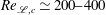 $Re_{\mathscr{L},c}\simeq 200{-}400$
.
$Re_{\mathscr{L},c}\simeq 200{-}400$
.
The comparison of the
 $Pr=5.0$
result of Taylor et al. (Reference Taylor, Sarkar and Armenio2005) to the present
$Pr=5.0$
result of Taylor et al. (Reference Taylor, Sarkar and Armenio2005) to the present
 $Pr=0.71$
study is not straightforward. The temperature scale
$Pr=0.71$
study is not straightforward. The temperature scale
 ${\rm\Delta}{\it\phi}$
across their flow is set by the surface heat flux so
${\rm\Delta}{\it\phi}$
across their flow is set by the surface heat flux so
 $\text{d}\langle {\it\phi}\rangle /\text{d}z\sim Pr$
. An approximate re-normalisation of their result is made here to our
$\text{d}\langle {\it\phi}\rangle /\text{d}z\sim Pr$
. An approximate re-normalisation of their result is made here to our
 $Pr=0.71$
values by
$Pr=0.71$
values by
 $Ri_{b}\times 0.71/5.0$
as indicated in figure 18. Their results compare reasonably well apart from
$Ri_{b}\times 0.71/5.0$
as indicated in figure 18. Their results compare reasonably well apart from
 ${\it\lambda}>0.1$
where, in their study, there is an increasingly thick diffusive region near the free surface, thereby increasing
${\it\lambda}>0.1$
where, in their study, there is an increasingly thick diffusive region near the free surface, thereby increasing
 ${\rm\Delta}{\it\phi}$
across the channel and hence
${\rm\Delta}{\it\phi}$
across the channel and hence
 $Ri_{b}$
. Our
$Ri_{b}$
. Our
 ${\it\alpha}{\it\delta}=32$
results behave in a similar manner.
${\it\alpha}{\it\delta}=32$
results behave in a similar manner.
In terms of
 $E_{r}$
, the critical values for the onset of stratified conditions, in coastal flows
$E_{r}$
, the critical values for the onset of stratified conditions, in coastal flows
 $E_{r,c}\simeq 0.003$
and river channels 0.0044 (Bormans & Webster Reference Bormans and Webster1997), corresponds to
$E_{r,c}\simeq 0.003$
and river channels 0.0044 (Bormans & Webster Reference Bormans and Webster1997), corresponds to
 ${\it\lambda}=0.05{-}0.1$
in the present study, indicating near-neutral flow conditions. The bulk parameter
${\it\lambda}=0.05{-}0.1$
in the present study, indicating near-neutral flow conditions. The bulk parameter
 $E_{r}$
contains an additional Reynolds number dependence through skin friction coefficient variation in
$E_{r}$
contains an additional Reynolds number dependence through skin friction coefficient variation in
 $E_{r}={\it\lambda}(C_{f}/2)^{1/2}$
, which is unrelated to the viscous parameter
$E_{r}={\it\lambda}(C_{f}/2)^{1/2}$
, which is unrelated to the viscous parameter
 $Re_{\mathscr{L}}$
. In our
$Re_{\mathscr{L}}$
. In our
 ${\it\lambda}=0.5$
result across
${\it\lambda}=0.5$
result across
 $Re_{{\it\tau}}=200{-}800$
there is variation over
$Re_{{\it\tau}}=200{-}800$
there is variation over
 $E_{r}=0.023{-}0.028$
(in table 1) while the behaviour is apparently consistent in terms of the kinetic energy budgets and turbulence intensities and consistent in terms of bulk
$E_{r}=0.023{-}0.028$
(in table 1) while the behaviour is apparently consistent in terms of the kinetic energy budgets and turbulence intensities and consistent in terms of bulk
 $Ri_{b}$
behaviour. We note that in translating critical flow parameter values from flow in coastal seas, where
$Ri_{b}$
behaviour. We note that in translating critical flow parameter values from flow in coastal seas, where
 $Re$
is
$Re$
is
 $O(10^{7})$
, to the smaller scale river flow considered in the present study, where
$O(10^{7})$
, to the smaller scale river flow considered in the present study, where
 $Re$
is
$Re$
is
 $O(10^{5})$
, the choice of parameter
$O(10^{5})$
, the choice of parameter
 $E_{r}$
or
$E_{r}$
or
 ${\it\lambda}$
may lead to considerable variation in predicted behaviour.
${\it\lambda}$
may lead to considerable variation in predicted behaviour.

Figure 19.
 $l_{m}{\it\delta}/R_{f}{\it\Lambda}$
for
$l_{m}{\it\delta}/R_{f}{\it\Lambda}$
for
 $Re_{{\it\tau}}=395$
with
$Re_{{\it\tau}}=395$
with
 ${\it\lambda}=0.05{-}2.0$
.
${\it\lambda}=0.05{-}2.0$
.
4.4. Parameterisation of turbulent mixing
Transition behaviour can be viewed in terms of turbulent mixing. Recent studies (Osborn Reference Osborn1980; Shih et al.
Reference Shih, Koseff, Ivey and Ferziger2005; Ivey et al.
Reference Ivey, Winters and Koseff2008; Gonzalez-Juez et al.
Reference Gonzalez-Juez, Kerstein and Shih2011; Chung & Matheou Reference Chung and Matheou2012) have suggested that the effects of buoyancy on turbulent mixing can be parameterised in terms of
 $\mathscr{R}$
. For
$\mathscr{R}$
. For
 $\mathscr{R}<\mathscr{R}_{c}$
the mixing is reduced to molecular levels or
$\mathscr{R}<\mathscr{R}_{c}$
the mixing is reduced to molecular levels or
 $k_{m}\rightarrow 0$
(Shih et al.
Reference Shih, Koseff, Ivey and Ferziger2005). For
$k_{m}\rightarrow 0$
(Shih et al.
Reference Shih, Koseff, Ivey and Ferziger2005). For
 $\mathscr{R}>\mathscr{R}_{c}$
Osborn (Reference Osborn1980) showed
$\mathscr{R}>\mathscr{R}_{c}$
Osborn (Reference Osborn1980) showed
 $k_{m}\leqslant {\it\epsilon}/N^{2}$
or
$k_{m}\leqslant {\it\epsilon}/N^{2}$
or
 $k_{m}/{\it\nu}\simeq {\it\Gamma}\mathscr{R}$
where
$k_{m}/{\it\nu}\simeq {\it\Gamma}\mathscr{R}$
where
 ${\it\Gamma}$
is the mixing efficiency. At large
${\it\Gamma}$
is the mixing efficiency. At large
 $\mathscr{R}$
the dependence of
$\mathscr{R}$
the dependence of
 $k_{m}$
on
$k_{m}$
on
 $\mathscr{R}$
decreases (Shih et al.
Reference Shih, Koseff, Ivey and Ferziger2005) and ultimately becomes independent of
$\mathscr{R}$
decreases (Shih et al.
Reference Shih, Koseff, Ivey and Ferziger2005) and ultimately becomes independent of
 $\mathscr{R}$
in neutral conditions (Chung & Matheou Reference Chung and Matheou2012).
$\mathscr{R}$
in neutral conditions (Chung & Matheou Reference Chung and Matheou2012).
The local mixing parameters can be re-cast in terms of
 ${\it\lambda}$
and
${\it\lambda}$
and
 $R_{f}$
. The non-dimensional mixing length
$R_{f}$
. The non-dimensional mixing length
 $$\begin{eqnarray}l_{m}=\langle u^{\prime }w^{\prime }\rangle ^{1/2}/S\end{eqnarray}$$
can be normalised with the
 $P-{\it\varepsilon}-B=0$
approximation to
$P-{\it\varepsilon}-B=0$
approximation to
 $$\begin{eqnarray}\frac{l_{m}}{R_{f}({\it\Lambda}/{\it\delta})}\simeq \frac{B+{\it\varepsilon}}{P}\simeq 1.0.\end{eqnarray}$$
This ratio, presented in figure 19, effectively demonstrates the range where local equilibrium holds. When
 $R_{f}\simeq R_{f,c}$
, then
$R_{f}\simeq R_{f,c}$
, then
 $l_{m}\sim {\it\Lambda}/{\it\delta}$
, consistent with limit conditions in Monin–Obukhov similarity models (Businger et al.
Reference Businger, Wyngaard, Izumi and Bradley1971; Chung & Matheou Reference Chung and Matheou2012). Garcia-Villalba & del Alamo (Reference Garcia-Villalba and del Alamo2011) showed that the local Obukhov length scale can be used to scale features of the turbulent two-dimensional velocity spectra in channel flow for
$l_{m}\sim {\it\Lambda}/{\it\delta}$
, consistent with limit conditions in Monin–Obukhov similarity models (Businger et al.
Reference Businger, Wyngaard, Izumi and Bradley1971; Chung & Matheou Reference Chung and Matheou2012). Garcia-Villalba & del Alamo (Reference Garcia-Villalba and del Alamo2011) showed that the local Obukhov length scale can be used to scale features of the turbulent two-dimensional velocity spectra in channel flow for
 ${\it\kappa}z/{\it\Lambda}\gtrsim 1$
, also consistent with our bulk parameter range for equilibrium
${\it\kappa}z/{\it\Lambda}\gtrsim 1$
, also consistent with our bulk parameter range for equilibrium
 ${\it\lambda}={\it\delta}/\mathscr{L}\gtrsim 1.0$
. The transition in mixing behaviour can also be seen in terms of the eddy viscosity ratio
${\it\lambda}={\it\delta}/\mathscr{L}\gtrsim 1.0$
. The transition in mixing behaviour can also be seen in terms of the eddy viscosity ratio
 $k_{m}/{\it\nu}$
,
$k_{m}/{\it\nu}$
,
 $$\begin{eqnarray}k_{m}/{\it\nu}\equiv \langle u^{\prime }w^{\prime }\rangle Re_{{\it\tau}}/S=Pr_{t}BRe_{{\it\tau}}/\mathscr{N}^{2}\simeq Pr_{t}{\it\Gamma}\mathscr{R}=R_{f}Re_{{\it\Lambda}},\end{eqnarray}$$
where the mixing efficiency is given as
 ${\it\Gamma}=B/{\it\varepsilon}\equiv R_{f}/(1-R_{f})$
. Vertical profiles of
${\it\Gamma}=B/{\it\varepsilon}\equiv R_{f}/(1-R_{f})$
. Vertical profiles of
 $k_{m}/{\it\nu}$
are given in figure 20 versus local values of
$k_{m}/{\it\nu}$
are given in figure 20 versus local values of
 $\mathscr{R}$
. The transition behaviour seen here through a sweep across the boundary layer height has the same behaviour as observed in the single-parameter-set simulations in homogeneous stratified shear flow of Shih et al. (Reference Shih, Koseff, Ivey and Ferziger2005) and Chung & Matheou (Reference Chung and Matheou2012). The
$\mathscr{R}$
. The transition behaviour seen here through a sweep across the boundary layer height has the same behaviour as observed in the single-parameter-set simulations in homogeneous stratified shear flow of Shih et al. (Reference Shih, Koseff, Ivey and Ferziger2005) and Chung & Matheou (Reference Chung and Matheou2012). The
 $Re_{{\it\tau}}=395$
results appear to asymptote to
$Re_{{\it\tau}}=395$
results appear to asymptote to
 $k_{m}/{\it\nu}=0.25\mathscr{R}$
at
$k_{m}/{\it\nu}=0.25\mathscr{R}$
at
 $\mathscr{R}\simeq 30$
while those at
$\mathscr{R}\simeq 30$
while those at
 $Re_{{\it\tau}}=800$
and
$Re_{{\it\tau}}=800$
and
 $Re_{{\it\tau}}=200$
transition at
$Re_{{\it\tau}}=200$
transition at
 $\mathscr{R}=60$
and
$\mathscr{R}=60$
and
 $\mathscr{R}=10{-}20$
. At higher
$\mathscr{R}=10{-}20$
. At higher
 $\mathscr{R}$
the flow approaches neutral behaviour with
$\mathscr{R}$
the flow approaches neutral behaviour with
 $k_{m}/{\it\nu}$
independent of
$k_{m}/{\it\nu}$
independent of
 $\mathscr{R}$
. There is an extended transition over
$\mathscr{R}$
. There is an extended transition over
 $\mathscr{R}$
of
$\mathscr{R}$
of
 $O(10)$
between these limits. In the small-
$O(10)$
between these limits. In the small-
 $\mathscr{R}$
limit, the asymptote
$\mathscr{R}$
limit, the asymptote
 $0.25\mathscr{R}$
indicates
$0.25\mathscr{R}$
indicates
 $\mathscr{R}=4$
as a limit for
$\mathscr{R}=4$
as a limit for
 $k_{m}/{\it\nu}\simeq 1$
in line with the
$k_{m}/{\it\nu}\simeq 1$
in line with the
 $\mathscr{R}=7$
value given by Shih et al. (Reference Shih, Koseff, Ivey and Ferziger2005).
$\mathscr{R}=7$
value given by Shih et al. (Reference Shih, Koseff, Ivey and Ferziger2005).

Figure 20. Variation of eddy viscosity ratio,
 $k_{m}/{\it\nu}$
, with
$k_{m}/{\it\nu}$
, with
 $\mathscr{R}$
at
$\mathscr{R}$
at
 $\mathit{Re}_{{\it\tau}}=395$
(a) and
$\mathit{Re}_{{\it\tau}}=395$
(a) and
 $\mathit{Re}_{{\it\tau}}=200{-}800$
(b). Straight solid line indicates
$\mathit{Re}_{{\it\tau}}=200{-}800$
(b). Straight solid line indicates
 $k_{m}/{\it\nu}=0.25\mathscr{R}$
.
$k_{m}/{\it\nu}=0.25\mathscr{R}$
.
5. Near-wall flow
In the near-wall region we have observed
 $Ri\ll Ri_{c}$
and
$Ri\ll Ri_{c}$
and
 $\mathscr{R}\gg 7$
, indicating only weakly stratified flow with wide separation of viscous and buoyancy scales, an observation reinforced by the very slight variation in the velocity profile, shear stress, normal stresses (figures 15–17) and TKE budget within this region with increasing
$\mathscr{R}\gg 7$
, indicating only weakly stratified flow with wide separation of viscous and buoyancy scales, an observation reinforced by the very slight variation in the velocity profile, shear stress, normal stresses (figures 15–17) and TKE budget within this region with increasing
 ${\it\lambda}$
. We can quantify this sensitivity (or lack thereof) more precisely by examining the scaling for the near-wall velocity profiles in the near-wall region with
${\it\lambda}$
. We can quantify this sensitivity (or lack thereof) more precisely by examining the scaling for the near-wall velocity profiles in the near-wall region with
 ${\it\lambda}$
and
${\it\lambda}$
and
 $Re_{{\it\tau}}$
.
$Re_{{\it\tau}}$
.
The relation
 ${\it\gamma}=z^{+}\text{d}u/\text{d}z^{+}$
is shown in figure 21 with vertical location in wall units. In a log-law region
${\it\gamma}=z^{+}\text{d}u/\text{d}z^{+}$
is shown in figure 21 with vertical location in wall units. In a log-law region
 ${\it\gamma}$
should be a constant
${\it\gamma}$
should be a constant
 $1/{\it\kappa}\simeq 2.44$
in neutral flow. The profiles correspond across the range of Reynolds numbers and
$1/{\it\kappa}\simeq 2.44$
in neutral flow. The profiles correspond across the range of Reynolds numbers and
 ${\it\lambda}$
for
${\it\lambda}$
for
 $z^{+}<30$
, within the viscous region, but there is rapid divergence with both quantities above this height. In the neutral case
$z^{+}<30$
, within the viscous region, but there is rapid divergence with both quantities above this height. In the neutral case
 ${\it\gamma}\simeq 2.5$
over
${\it\gamma}\simeq 2.5$
over
 $z^{+}=50{-}75$
, which is somewhat higher than the closed channel flow
$z^{+}=50{-}75$
, which is somewhat higher than the closed channel flow
 $Re_{{\it\tau}}=392$
result of Moser et al. (Reference Moser, Kim and Mansour1999) but suggests a short region where the log law holds. In the stratified flows there is a consistent increase in
$Re_{{\it\tau}}=392$
result of Moser et al. (Reference Moser, Kim and Mansour1999) but suggests a short region where the log law holds. In the stratified flows there is a consistent increase in
 ${\it\gamma}$
with
${\it\gamma}$
with
 ${\it\lambda}$
for
${\it\lambda}$
for
 $z^{+}>30$
. It is clear from figure 21 that the inner wall region is influenced by stratification, albeit significantly less than in previous stratified wall studies such as Garcia-Villalba & del Alamo (Reference Garcia-Villalba and del Alamo2011) as suggested by their observed near-wall re-laminarisation events and larger near-wall buoyancy flux.
$z^{+}>30$
. It is clear from figure 21 that the inner wall region is influenced by stratification, albeit significantly less than in previous stratified wall studies such as Garcia-Villalba & del Alamo (Reference Garcia-Villalba and del Alamo2011) as suggested by their observed near-wall re-laminarisation events and larger near-wall buoyancy flux.

Figure 21. Log-law constant,
 ${\it\gamma}=z^{+}\text{d}u/\text{d}z^{+}$
. Thin horizontal line indicates
${\it\gamma}=z^{+}\text{d}u/\text{d}z^{+}$
. Thin horizontal line indicates
 $1/{\it\kappa}=2.44$
. Closed channel flow data of Moser et al. (Reference Moser, Kim and Mansour1999) at
$1/{\it\kappa}=2.44$
. Closed channel flow data of Moser et al. (Reference Moser, Kim and Mansour1999) at
 $Re=392$
indicated for comparison.
$Re=392$
indicated for comparison.
The
 ${\it\lambda}=0.5$
result at
${\it\lambda}=0.5$
result at
 $Re_{{\it\tau}}=800$
lies between the
$Re_{{\it\tau}}=800$
lies between the
 ${\it\lambda}=0$
and 0.1 results at
${\it\lambda}=0$
and 0.1 results at
 $Re_{{\it\tau}}=395$
out to
$Re_{{\it\tau}}=395$
out to
 $z^{+}\simeq 200$
, considerably lower than the
$z^{+}\simeq 200$
, considerably lower than the
 ${\it\lambda}=0.5$
result at
${\it\lambda}=0.5$
result at
 $Re_{{\it\tau}}=395$
. At the Reynolds numbers used here, there are expected to be low-Reynolds-number effects leading to variation in
$Re_{{\it\tau}}=395$
. At the Reynolds numbers used here, there are expected to be low-Reynolds-number effects leading to variation in
 ${\it\gamma}$
even in the neutral case (Moser et al.
Reference Moser, Kim and Mansour1999); however, the greater part of this variation is due to the differing near-wall scaling of the shear stress and buoyancy flux profiles. The buoyancy flux
${\it\gamma}$
even in the neutral case (Moser et al.
Reference Moser, Kim and Mansour1999); however, the greater part of this variation is due to the differing near-wall scaling of the shear stress and buoyancy flux profiles. The buoyancy flux
 $B=-{\it\lambda}\langle {\it\phi}^{\prime }w^{\prime }\rangle$
profile varies with
$B=-{\it\lambda}\langle {\it\phi}^{\prime }w^{\prime }\rangle$
profile varies with
 $z$
expressed in outer layer units, while by definition the beginning of the apparent log-law behaviour at
$z$
expressed in outer layer units, while by definition the beginning of the apparent log-law behaviour at
 $z^{+}\simeq 50$
scales with viscous wall units (
$z^{+}\simeq 50$
scales with viscous wall units (
 $z^{+}=zRe_{{\it\tau}}$
). Over the near-wall region there is a near linear decrease in
$z^{+}=zRe_{{\it\tau}}$
). Over the near-wall region there is a near linear decrease in
 $B$
to
$B$
to
 $z=0$
,
$z=0$
,
 $B=0$
(figure 9), so at fixed
$B=0$
(figure 9), so at fixed
 $z^{+}$
,
$z^{+}$
,
 $B$
is inversely proportional to Reynolds number.
$B$
is inversely proportional to Reynolds number.
This Reynolds number influence can also be seen in the scaling for
 $\mathscr{R}$
profiles in the near-wall region. We obtain the scaling
$\mathscr{R}$
profiles in the near-wall region. We obtain the scaling
 $\mathscr{R}\sim Re_{{\it\Lambda}}$
from (4.4), which holds where there is energetic equilibrium, including the log-law region as shown in figure 10(a). From definitions in (1.7b
) and (1.10b
) we can write in non-dimensional form
$\mathscr{R}\sim Re_{{\it\Lambda}}$
from (4.4), which holds where there is energetic equilibrium, including the log-law region as shown in figure 10(a). From definitions in (1.7b
) and (1.10b
) we can write in non-dimensional form
 $Re_{{\it\Lambda}}(z)=-\langle u^{\prime }w^{\prime }\rangle ^{2}Re_{{\it\tau}}/{\it\lambda}\langle {\it\phi}^{\prime }w^{\prime }\rangle$
and re-arrange to obtain
$Re_{{\it\Lambda}}(z)=-\langle u^{\prime }w^{\prime }\rangle ^{2}Re_{{\it\tau}}/{\it\lambda}\langle {\it\phi}^{\prime }w^{\prime }\rangle$
and re-arrange to obtain
 $Re_{{\it\Lambda}}(z)=-Re_{\mathscr{L}}\langle u^{\prime }w^{\prime }\rangle ^{2}/\langle {\it\phi}^{\prime }w^{\prime }\rangle$
. In the lower log-law region, say at
$Re_{{\it\Lambda}}(z)=-Re_{\mathscr{L}}\langle u^{\prime }w^{\prime }\rangle ^{2}/\langle {\it\phi}^{\prime }w^{\prime }\rangle$
. In the lower log-law region, say at
 $z^{+}=50$
,
$z^{+}=50$
,
 $\langle u^{\prime }w^{\prime }\rangle \simeq u_{{\it\tau}}\simeq 1$
while the buoyancy flux
$\langle u^{\prime }w^{\prime }\rangle \simeq u_{{\it\tau}}\simeq 1$
while the buoyancy flux
 $-\langle {\it\phi}^{\prime }w^{\prime }\rangle \simeq z(I_{s}/{\it\delta}q_{N})$
from (3.2). In wall units then
$-\langle {\it\phi}^{\prime }w^{\prime }\rangle \simeq z(I_{s}/{\it\delta}q_{N})$
from (3.2). In wall units then
 $-\langle {\it\phi}^{\prime }w^{\prime }\rangle \simeq z^{+}(I_{s}/{\it\delta}q_{N})/Re_{{\it\tau}}$
so
$-\langle {\it\phi}^{\prime }w^{\prime }\rangle \simeq z^{+}(I_{s}/{\it\delta}q_{N})/Re_{{\it\tau}}$
so
 $Re_{{\it\Lambda}}(z^{+})\sim Re_{\mathscr{L}}Re_{{\it\tau}}/z^{+}(I_{s}/{\it\delta}q_{N})$
and
$Re_{{\it\Lambda}}(z^{+})\sim Re_{\mathscr{L}}Re_{{\it\tau}}/z^{+}(I_{s}/{\it\delta}q_{N})$
and
 $\mathscr{R}\sim Re_{\mathscr{L}}Re_{{\it\tau}}$
.
$\mathscr{R}\sim Re_{\mathscr{L}}Re_{{\it\tau}}$
.
This sensitivity is apparent in the
 $\mathscr{R}$
profiles for
$\mathscr{R}$
profiles for
 ${\it\lambda}=0.5$
in figure 14(b). At
${\it\lambda}=0.5$
in figure 14(b). At
 $z=0.05$
, at
$z=0.05$
, at
 $Re_{{\it\tau}}=200$
,
$Re_{{\it\tau}}=200$
,
 $\mathscr{R}\simeq 825$
, at
$\mathscr{R}\simeq 825$
, at
 $Re_{{\it\tau}}=395$
,
$Re_{{\it\tau}}=395$
,
 $\mathscr{R}\simeq 3636$
and at
$\mathscr{R}\simeq 3636$
and at
 $Re_{{\it\tau}}=800$
,
$Re_{{\it\tau}}=800$
,
 $\mathscr{R}\simeq 13\,937$
, giving a factor of 4.4 and 3.8 between these values, approximately in line with this scaling. The
$\mathscr{R}\simeq 13\,937$
, giving a factor of 4.4 and 3.8 between these values, approximately in line with this scaling. The
 ${\it\lambda}=1.0$
,
${\it\lambda}=1.0$
,
 $Re_{{\it\tau}}=395~(Re_{\mathscr{L}}=395)$
and
$Re_{{\it\tau}}=395~(Re_{\mathscr{L}}=395)$
and
 ${\it\lambda}=0.5$
,
${\it\lambda}=0.5$
,
 $Re_{{\it\tau}}=200$
(
$Re_{{\it\tau}}=200$
(
 $Re_{\mathscr{L}}=400$
) cases converge at
$Re_{\mathscr{L}}=400$
) cases converge at
 $z\simeq 0.3$
suggesting the limit of this behaviour in line with the outer extent of the log-law region in high-Reynolds-number neutral flow (Pope Reference Pope2000). Similar sensitivity is also seen in the
$z\simeq 0.3$
suggesting the limit of this behaviour in line with the outer extent of the log-law region in high-Reynolds-number neutral flow (Pope Reference Pope2000). Similar sensitivity is also seen in the
 ${\it\gamma}$
profiles in the near-wall region. The profile of
${\it\gamma}$
profiles in the near-wall region. The profile of
 ${\it\gamma}$
at
${\it\gamma}$
at
 ${\it\lambda}=0.5$
,
${\it\lambda}=0.5$
,
 $Re_{{\it\tau}}=800$
is close to that at
$Re_{{\it\tau}}=800$
is close to that at
 ${\it\lambda}=0.1$
for
${\it\lambda}=0.1$
for
 $Re_{{\it\tau}}=395$
, suggesting that halving of
$Re_{{\it\tau}}=395$
, suggesting that halving of
 $Re_{{\it\tau}}$
is equivalent to approximately a five-fold increase in
$Re_{{\it\tau}}$
is equivalent to approximately a five-fold increase in
 ${\it\lambda}$
.
${\it\lambda}$
.
This scaling contrasts with stratified wall flows where
 $-\langle {\it\phi}^{\prime }w^{\prime }\rangle \simeq (I_{s}/{\it\delta}q_{N})$
, that is with no
$-\langle {\it\phi}^{\prime }w^{\prime }\rangle \simeq (I_{s}/{\it\delta}q_{N})$
, that is with no
 $z$
dependence in the outer layer, so
$z$
dependence in the outer layer, so
 $\mathscr{R}\sim Re_{\mathscr{L}}$
.
$\mathscr{R}\sim Re_{\mathscr{L}}$
.
6. Scaling for free-surface affected region
In neutral conditions, the free surface affects the flow structure over a distance related to the integral length scale,
 $l_{\infty }$
, below the surface (Hunt & Graham Reference Hunt and Graham1978; Calmet & Magnaudet Reference Calmet and Magnaudet2003). Calmet & Magnaudet (Reference Calmet and Magnaudet2003) estimated
$l_{\infty }$
, below the surface (Hunt & Graham Reference Hunt and Graham1978; Calmet & Magnaudet Reference Calmet and Magnaudet2003). Calmet & Magnaudet (Reference Calmet and Magnaudet2003) estimated
 $l_{\infty }/{\it\delta}\sim 0.2$
and showed that this region coincides with the diverging near-surface profiles of
$l_{\infty }/{\it\delta}\sim 0.2$
and showed that this region coincides with the diverging near-surface profiles of
 $u_{rms}$
and
$u_{rms}$
and
 $w_{rms}$
. In our neutral flow results, the wall-normal turbulent intensity shown in figure 16(a), decreases at a faster rate above
$w_{rms}$
. In our neutral flow results, the wall-normal turbulent intensity shown in figure 16(a), decreases at a faster rate above
 $z\simeq 0.8$
, indicative of this region.
$z\simeq 0.8$
, indicative of this region.
Hunt & Graham (Reference Hunt and Graham1978) treated this region as a ‘source layer’, which supplied turbulence to an inner viscous sub-layer. This inner layer is characterised by a length scale
 $l_{{\it\nu}}$
, which has the scaling
$l_{{\it\nu}}$
, which has the scaling
 $l_{{\it\nu}}/l_{\infty }=O(Re_{\infty }^{-1/2})$
, where the Reynolds number can be defined
$l_{{\it\nu}}/l_{\infty }=O(Re_{\infty }^{-1/2})$
, where the Reynolds number can be defined
 $Re_{\infty }=l_{\infty }u/{\it\nu}$
(Hunt & Graham Reference Hunt and Graham1978; Hunt Reference Hunt, Brutseart and Jirka1984; Calmet & Magnaudet Reference Calmet and Magnaudet2003). Calmet & Magnaudet (Reference Calmet and Magnaudet2003) showed that the velocity scale can be taken as the wall friction velocity since the magnitude of the turbulence intensity at the surface is relatively insensitive to Reynolds number and is
$Re_{\infty }=l_{\infty }u/{\it\nu}$
(Hunt & Graham Reference Hunt and Graham1978; Hunt Reference Hunt, Brutseart and Jirka1984; Calmet & Magnaudet Reference Calmet and Magnaudet2003). Calmet & Magnaudet (Reference Calmet and Magnaudet2003) showed that the velocity scale can be taken as the wall friction velocity since the magnitude of the turbulence intensity at the surface is relatively insensitive to Reynolds number and is
 $O(u_{{\it\tau}})$
. This is seen in our neutral flow results where the streamwise turbulence intensity at the surface has a value of
$O(u_{{\it\tau}})$
. This is seen in our neutral flow results where the streamwise turbulence intensity at the surface has a value of
 $\langle uu^{\prime }\rangle ^{1/2}=0.91$
, the same as found by Calmet & Magnaudet (Reference Calmet and Magnaudet2003) at
$\langle uu^{\prime }\rangle ^{1/2}=0.91$
, the same as found by Calmet & Magnaudet (Reference Calmet and Magnaudet2003) at
 $Re_{{\it\tau}}=1280$
, and close to
$Re_{{\it\tau}}=1280$
, and close to
 $u_{{\it\tau}}=1$
.
$u_{{\it\tau}}=1$
.

Figure 22. Variation of near-surface profiles of
 $\mathscr{R}$
with
$\mathscr{R}$
with
 $(1-z)Re^{1/2}$
with vertical line indicating
$(1-z)Re^{1/2}$
with vertical line indicating
 $(1-z)Re^{1/2}=0.9$
.
$(1-z)Re^{1/2}=0.9$
.
The Reynolds number sensitivity is suggested in the spanwise and streamwise turbulence intensity profiles of our neutral flow results shown in figures 15(a) and 17(a). The spanwise stress
 $\langle v^{\prime }v^{\prime }\rangle ^{1/2}$
reaches a minimum value at
$\langle v^{\prime }v^{\prime }\rangle ^{1/2}$
reaches a minimum value at
 $z=0.9$
while Calmet & Magnaudet (Reference Calmet and Magnaudet2003) reported
$z=0.9$
while Calmet & Magnaudet (Reference Calmet and Magnaudet2003) reported
 $z=0.925$
at
$z=0.925$
at
 $Re_{{\it\tau}}=1280$
and Handler et al. (Reference Handler, Saylor, Leighton and Rovelstad1999)
$Re_{{\it\tau}}=1280$
and Handler et al. (Reference Handler, Saylor, Leighton and Rovelstad1999)
 $z=0.83{-}0.9$
at
$z=0.83{-}0.9$
at
 $Re_{{\it\tau}}=180$
.
$Re_{{\it\tau}}=180$
.
The Reynolds number dependence appears to be maintained even at high levels of stratification. At
 ${\it\lambda}=0.5$
, the intensity
${\it\lambda}=0.5$
, the intensity
 $\langle v^{\prime }v^{\prime }\rangle ^{1/2}$
reaches minimum near-surface values at
$\langle v^{\prime }v^{\prime }\rangle ^{1/2}$
reaches minimum near-surface values at
 $z=0.938$
, 0.955 and 0.968 at
$z=0.938$
, 0.955 and 0.968 at
 $Re_{{\it\tau}}=200$
,
$Re_{{\it\tau}}=200$
,
 $Re_{{\it\tau}}=395$
and
$Re_{{\it\tau}}=395$
and
 $Re_{{\it\tau}}=800$
respectively. There is also little variation in the magnitude of intensities through the near-surface region with Reynolds number, with the surface values of
$Re_{{\it\tau}}=800$
respectively. There is also little variation in the magnitude of intensities through the near-surface region with Reynolds number, with the surface values of
 $\langle u^{\prime }u^{\prime }\rangle ^{1/2}$
being 0.65 and 0.66 at
$\langle u^{\prime }u^{\prime }\rangle ^{1/2}$
being 0.65 and 0.66 at
 $Re_{{\it\tau}}=395$
and 800 respectively.
$Re_{{\it\tau}}=395$
and 800 respectively.
Calmet & Magnaudet (Reference Calmet and Magnaudet2003) found
 $l_{{\it\nu}}\simeq 2Re_{\infty }^{-1/2}l_{\infty }$
, determined by locating the near-surface peak in r.m.s. vorticity. Taking the integral length scale to be
$l_{{\it\nu}}\simeq 2Re_{\infty }^{-1/2}l_{\infty }$
, determined by locating the near-surface peak in r.m.s. vorticity. Taking the integral length scale to be
 $l_{\infty }/{\it\delta}\sim 0.2$
and
$l_{\infty }/{\it\delta}\sim 0.2$
and
 $Re_{\infty }=Re_{{\it\tau}}l_{\infty }/{\it\delta}$
, this scaling indicates
$Re_{\infty }=Re_{{\it\tau}}l_{\infty }/{\it\delta}$
, this scaling indicates
 $l_{{\it\nu}}/{\it\delta}\simeq 0.04$
at
$l_{{\it\nu}}/{\it\delta}\simeq 0.04$
at
 $Re_{{\it\tau}}=395$
. We examine the near-surface behaviour of our results using the
$Re_{{\it\tau}}=395$
. We examine the near-surface behaviour of our results using the
 $\mathscr{R}$
profiles in figure 22. We have scaled the near-surface distance
$\mathscr{R}$
profiles in figure 22. We have scaled the near-surface distance
 $(1-z)$
with
$(1-z)$
with
 $Re^{1/2}$
. In all the data sets shown, there is a location of minimum
$Re^{1/2}$
. In all the data sets shown, there is a location of minimum
 $\mathscr{R}$
just below the surface which appears to scale to
$\mathscr{R}$
just below the surface which appears to scale to
 $(1-z)Re^{1/2}=0.9$
. For
$(1-z)Re^{1/2}=0.9$
. For
 $Re_{{\it\tau}}=395$
this location gives
$Re_{{\it\tau}}=395$
this location gives
 $(1-z)=0.045$
, approximately the same as the
$(1-z)=0.045$
, approximately the same as the
 $l_{{\it\nu}}/{\it\delta}\simeq 0.04$
estimate.
$l_{{\it\nu}}/{\it\delta}\simeq 0.04$
estimate.
This Reynolds number influence can also be seen in the energy balance ratio
 $P/({\it\varepsilon}+B)$
plotted in figure 23(a). Here we show results at
$P/({\it\varepsilon}+B)$
plotted in figure 23(a). Here we show results at
 ${\it\lambda}=0.5$
over the Reynolds number range
${\it\lambda}=0.5$
over the Reynolds number range
 $Re_{{\it\tau}}=200{-}800$
. The near-surface
$Re_{{\it\tau}}=200{-}800$
. The near-surface
 $(1-z)Re_{{\it\tau}}^{1/2}$
scaling appears to collapse the three curves over
$(1-z)Re_{{\it\tau}}^{1/2}$
scaling appears to collapse the three curves over
 $(1-z)Re_{{\it\tau}}^{1/2}\simeq 0{-}2$
. This corresponds to
$(1-z)Re_{{\it\tau}}^{1/2}\simeq 0{-}2$
. This corresponds to
 $(1-z)\simeq 0.1$
at
$(1-z)\simeq 0.1$
at
 $Re_{{\it\tau}}=395$
, approximately twice the estimated
$Re_{{\it\tau}}=395$
, approximately twice the estimated
 $l_{{\it\nu}}$
in neutral flow, suggesting a wider length over which the
$l_{{\it\nu}}$
in neutral flow, suggesting a wider length over which the
 $l_{{\it\nu}}$
scaling is relevant.
$l_{{\it\nu}}$
scaling is relevant.

Figure 23. Turbulent kinetic energy production as a ratio of total dissipation
 $P/({\it\varepsilon}+B)$
at
$P/({\it\varepsilon}+B)$
at
 $\mathit{Re}_{{\it\tau}}=200{-}800$
, with location from free surface
$\mathit{Re}_{{\it\tau}}=200{-}800$
, with location from free surface
 $(1-z)$
normalised by
$(1-z)$
normalised by
 $Re_{{\it\tau}}^{1/2}$
.
$Re_{{\it\tau}}^{1/2}$
.
Calmet & Magnaudet (Reference Calmet and Magnaudet2003) argued that the evolution of near-surface vorticity can be related to the Taylor micro-scale
 $l_{t}$
, noting that
$l_{t}$
, noting that
 $l_{t}/l_{\infty }\sim Re_{\infty }^{-1/2}$
, the same as the
$l_{t}/l_{\infty }\sim Re_{\infty }^{-1/2}$
, the same as the
 $l_{{\it\nu}}/l_{\infty }$
scaling of Hunt & Graham (Reference Hunt and Graham1978). We can consider the effect of buoyancy on the near-surface
$l_{{\it\nu}}/l_{\infty }$
scaling of Hunt & Graham (Reference Hunt and Graham1978). We can consider the effect of buoyancy on the near-surface
 $l_{{\it\nu}}$
scaling through extension of these Taylor micro-scale arguments. Using dimensional variables, the Taylor micro-scale is defined
$l_{{\it\nu}}$
scaling through extension of these Taylor micro-scale arguments. Using dimensional variables, the Taylor micro-scale is defined
 $l_{t}^{2}={\it\nu}\langle u^{2}\rangle /{\it\epsilon}$
, where
$l_{t}^{2}={\it\nu}\langle u^{2}\rangle /{\it\epsilon}$
, where
 ${\it\epsilon}$
is the dimensional dissipation rate of TKE. The neutral flow turbulence intensities and the dissipation rate are nearly constant with Reynolds number in the near-surface region. In stratified flow, however,
${\it\epsilon}$
is the dimensional dissipation rate of TKE. The neutral flow turbulence intensities and the dissipation rate are nearly constant with Reynolds number in the near-surface region. In stratified flow, however,
 ${\it\epsilon}$
will vary. In stratified flow we can relate the buoyancy flux to the dissipation rate with the definition of mixing efficiency,
${\it\epsilon}$
will vary. In stratified flow we can relate the buoyancy flux to the dissipation rate with the definition of mixing efficiency,
 ${\it\epsilon}=\langle b^{\prime }w^{\prime }\rangle /{\it\Gamma}$
, to obtain
${\it\epsilon}=\langle b^{\prime }w^{\prime }\rangle /{\it\Gamma}$
, to obtain
 $l_{t}^{2}={\it\nu}\langle u^{2}\rangle {\it\Gamma}/\langle b^{\prime }w^{\prime }\rangle$
.
$l_{t}^{2}={\it\nu}\langle u^{2}\rangle {\it\Gamma}/\langle b^{\prime }w^{\prime }\rangle$
.
If we adopt
 $u_{rms}$
as the velocity scale, and note from figure 15(a) that at the approximate boundary of the source layer
$u_{rms}$
as the velocity scale, and note from figure 15(a) that at the approximate boundary of the source layer
 $z\simeq 0.8$
,
$z\simeq 0.8$
,
 $u_{rms}/u_{{\it\tau}}\simeq 1$
, we obtain
$u_{rms}/u_{{\it\tau}}\simeq 1$
, we obtain
 $l_{t}^{2}\simeq {\it\nu}{\it\Gamma}u_{{\it\tau}}^{2}/\langle b^{\prime }w^{\prime }\rangle$
. We can use the relations
$l_{t}^{2}\simeq {\it\nu}{\it\Gamma}u_{{\it\tau}}^{2}/\langle b^{\prime }w^{\prime }\rangle$
. We can use the relations
 ${\it\Lambda}=\langle u^{\prime }w^{\prime }\rangle ^{3/2}/\langle b^{\prime }w^{\prime }\rangle$
and
${\it\Lambda}=\langle u^{\prime }w^{\prime }\rangle ^{3/2}/\langle b^{\prime }w^{\prime }\rangle$
and
 $u_{{\it\tau}}^{2}\simeq \langle u^{\prime }w^{\prime }\rangle$
to obtain
$u_{{\it\tau}}^{2}\simeq \langle u^{\prime }w^{\prime }\rangle$
to obtain
 $l_{t}^{2}\simeq {\it\nu}{\it\Gamma}{\it\Lambda}/u_{{\it\tau}}$
. Here we are essentially arguing that the flow near the surface is characterised by the properties of the turbulence, transported into the source layer from the stratified boundary layer, at
$l_{t}^{2}\simeq {\it\nu}{\it\Gamma}{\it\Lambda}/u_{{\it\tau}}$
. Here we are essentially arguing that the flow near the surface is characterised by the properties of the turbulence, transported into the source layer from the stratified boundary layer, at
 $z\simeq 0.8$
.
$z\simeq 0.8$
.
In non-dimensional form this becomes
 $l_{t}^{2}/{\it\delta}^{2}\simeq {\it\Gamma}{\it\Lambda}/{\it\delta}Re_{{\it\tau}}$
. The local Obukhov length scales with
$l_{t}^{2}/{\it\delta}^{2}\simeq {\it\Gamma}{\it\Lambda}/{\it\delta}Re_{{\it\tau}}$
. The local Obukhov length scales with
 ${\it\Lambda}/{\it\delta}\sim 1/{\it\lambda}$
so we can obtain the scaling
${\it\Lambda}/{\it\delta}\sim 1/{\it\lambda}$
so we can obtain the scaling
 $l_{t}/{\it\delta}\sim {\it\Gamma}^{1/2}(Re_{{\it\tau}}{\it\lambda})^{-1/2}$
. In this relationship
$l_{t}/{\it\delta}\sim {\it\Gamma}^{1/2}(Re_{{\it\tau}}{\it\lambda})^{-1/2}$
. In this relationship
 ${\it\Gamma}$
is an unknown property of the turbulence. In very stable flow, however, limit conditions are approached. In figure 10(c) we have seen that
${\it\Gamma}$
is an unknown property of the turbulence. In very stable flow, however, limit conditions are approached. In figure 10(c) we have seen that
 $R_{f}\rightarrow R_{f,c}$
at
$R_{f}\rightarrow R_{f,c}$
at
 $z\simeq 0.8$
for
$z\simeq 0.8$
for
 ${\it\lambda}\gtrsim 0.5$
. This implies
${\it\lambda}\gtrsim 0.5$
. This implies
 ${\it\Gamma}\rightarrow {\it\Gamma}_{c}$
under strong stable conditions so the scaling can be reduced to
${\it\Gamma}\rightarrow {\it\Gamma}_{c}$
under strong stable conditions so the scaling can be reduced to
 $l_{t}/{\it\delta}\sim (Re_{{\it\tau}}{\it\lambda})^{-1/2}$
.
$l_{t}/{\it\delta}\sim (Re_{{\it\tau}}{\it\lambda})^{-1/2}$
.
It is clear that in the inner layer the
 $\mathscr{R}$
behaviour does not have this character in figure 22 but we note that in the spanwise turbulence intensity profile shown in figure 17(a) there is a location in the surface region where intensity
$\mathscr{R}$
behaviour does not have this character in figure 22 but we note that in the spanwise turbulence intensity profile shown in figure 17(a) there is a location in the surface region where intensity
 $\text{d}\langle v^{\prime }v^{\prime }\rangle /\text{d}z=0$
and that this location has a
$\text{d}\langle v^{\prime }v^{\prime }\rangle /\text{d}z=0$
and that this location has a
 ${\it\lambda}$
sensitivity, particularly for
${\it\lambda}$
sensitivity, particularly for
 ${\it\lambda}=0.05{-}0.2$
. In these cases, however,
${\it\lambda}=0.05{-}0.2$
. In these cases, however,
 ${\it\Gamma}$
is varying significantly with
${\it\Gamma}$
is varying significantly with
 ${\it\lambda}$
and
${\it\lambda}$
and
 $z$
at
$z$
at
 $z\simeq 0.8$
(see
$z\simeq 0.8$
(see
 $R_{f}$
in figure 10
c) making any comparison unsatisfactory. For
$R_{f}$
in figure 10
c) making any comparison unsatisfactory. For
 ${\it\lambda}\geqslant 1.0$
,
${\it\lambda}\geqslant 1.0$
,
 $\mathscr{R}<\mathscr{R}_{c}$
near
$\mathscr{R}<\mathscr{R}_{c}$
near
 $z\simeq 0.8$
signifying the onset of the diffusive regime.
$z\simeq 0.8$
signifying the onset of the diffusive regime.
In summary we are not able to report convincing evidence for the
 ${\it\lambda}$
sensitivity of this scaling but can report that the Reynolds number dependence is maintained in the same way as seen in neutral flow.
${\it\lambda}$
sensitivity of this scaling but can report that the Reynolds number dependence is maintained in the same way as seen in neutral flow.
7. Conclusions
We have examined turbulent stratified open channel flow. Our buoyancy bulk parameter is defined through the ratio of the domain height
 ${\it\delta}$
to
${\it\delta}$
to
 $\mathscr{L}$
, denoted
$\mathscr{L}$
, denoted
 ${\it\lambda}$
, a bulk Obukhov length scale for the flow, covering the range
${\it\lambda}$
, a bulk Obukhov length scale for the flow, covering the range
 ${\it\delta}/\mathscr{L}=0{-}2.0$
at
${\it\delta}/\mathscr{L}=0{-}2.0$
at
 $Re_{{\it\tau}}=395$
. We obtain a boundary layer flow where the effects of stratification are weak in the near-wall region but progressively stronger in the outer layer up to the free surface.
$Re_{{\it\tau}}=395$
. We obtain a boundary layer flow where the effects of stratification are weak in the near-wall region but progressively stronger in the outer layer up to the free surface.
With increasing flow stability, two significant changes occur in the flow. Firstly the flow becomes local for
 ${\it\lambda}\gtrsim 0.5$
, with turbulence production and dissipation in local equilibrium,
${\it\lambda}\gtrsim 0.5$
, with turbulence production and dissipation in local equilibrium,
 $P/({\it\varepsilon}+B)\sim 1$
, extending from the near-wall region,
$P/({\it\varepsilon}+B)\sim 1$
, extending from the near-wall region,
 $z^{+}>50$
, to a near-surface limit, which we find is characterised by the same near-surface scaling as in neutral flow. For fixed
$z^{+}>50$
, to a near-surface limit, which we find is characterised by the same near-surface scaling as in neutral flow. For fixed
 ${\it\lambda}=0.5$
this length is
${\it\lambda}=0.5$
this length is
 $(1-z)Re_{{\it\tau}}^{1/2}\simeq 2$
. In this equilibrium region the flow can be characterised in terms of the flux Richardson number
$(1-z)Re_{{\it\tau}}^{1/2}\simeq 2$
. In this equilibrium region the flow can be characterised in terms of the flux Richardson number
 $R_{f}$
and the local Obukhov length scale
$R_{f}$
and the local Obukhov length scale
 ${\it\Lambda}$
; for example, a mixing length can be defined as
${\it\Lambda}$
; for example, a mixing length can be defined as
 $l_{m}\simeq R_{f}{\it\Lambda}/{\it\delta}$
. Above
$l_{m}\simeq R_{f}{\it\Lambda}/{\it\delta}$
. Above
 ${\it\lambda}\simeq 1.0$
, limit values for flux Richardson number
${\it\lambda}\simeq 1.0$
, limit values for flux Richardson number
 $R_{f}=R_{f,c}\simeq 0.17{-}0.2$
and
$R_{f}=R_{f,c}\simeq 0.17{-}0.2$
and
 $Ri=Ri_{c}\simeq 0.2$
are obtained over a fraction of the channel height. We find that the critical buoyancy parameter
$Ri=Ri_{c}\simeq 0.2$
are obtained over a fraction of the channel height. We find that the critical buoyancy parameter
 $E_{r,c}$
is not as general as
$E_{r,c}$
is not as general as
 ${\it\lambda}$
as it contains a Reynolds number dependence in
${\it\lambda}$
as it contains a Reynolds number dependence in
 $C_{f}$
.
$C_{f}$
.
At higher
 ${\it\lambda}$
we obtain a flow field where buoyancy interacts with the smallest scales of motion. We find that this regime can be identified by the parameter
${\it\lambda}$
we obtain a flow field where buoyancy interacts with the smallest scales of motion. We find that this regime can be identified by the parameter
 $Re_{\mathscr{L},c}=\mathscr{L}u_{{\it\tau}}/{\it\nu}\lesssim 200{-}400$
, which is related to the
$Re_{\mathscr{L},c}=\mathscr{L}u_{{\it\tau}}/{\it\nu}\lesssim 200{-}400$
, which is related to the
 $L_{\ast }$
parameter of Flores & Riley (Reference Flores and Riley2011). In the energetic equilibrium, the local buoyancy Reynolds number
$L_{\ast }$
parameter of Flores & Riley (Reference Flores and Riley2011). In the energetic equilibrium, the local buoyancy Reynolds number
 $Re_{{\it\Lambda}}={\it\Lambda}u_{{\it\tau}}/{\it\nu}$
is related directly to the separation of
$Re_{{\it\Lambda}}={\it\Lambda}u_{{\it\tau}}/{\it\nu}$
is related directly to the separation of
 $l_{O}$
and
$l_{O}$
and
 ${\it\eta}$
in the outer boundary layer by
${\it\eta}$
in the outer boundary layer by
 $Re_{{\it\Lambda}}\simeq \mathscr{R}\equiv (l_{O}/{\it\eta})^{4/3}$
. We observed that a consequence of the inhomogeneity of this flow appears to be that regions of
$Re_{{\it\Lambda}}\simeq \mathscr{R}\equiv (l_{O}/{\it\eta})^{4/3}$
. We observed that a consequence of the inhomogeneity of this flow appears to be that regions of
 $Ri\gg Ri_{c}$
are obtained where the flow is turbulent and
$Ri\gg Ri_{c}$
are obtained where the flow is turbulent and
 $\mathscr{R}\gg \mathscr{R}_{c}$
.
$\mathscr{R}\gg \mathscr{R}_{c}$
.
An interesting feature of this configuration is that statistically steady flow can be attained in relatively small computational domain sizes, unlike previously reported stratified boundary layer flows. The apparent difference here is that the near-wall region appears only subtly affected by stratification with
 $\mathscr{R}\sim Re_{\mathscr{L}}Re_{{\it\tau}}$
, in contrast to flows where buoyancy flux is non-zero at the wall and
$\mathscr{R}\sim Re_{\mathscr{L}}Re_{{\it\tau}}$
, in contrast to flows where buoyancy flux is non-zero at the wall and
 $\mathscr{R}\sim Re_{\mathscr{L}}$
.
$\mathscr{R}\sim Re_{\mathscr{L}}$
.
Acknowledgements
The authors gratefully acknowledge the support of the Australian Research Council (ARC). The first author was supported by ARC Post-doctoral Research Fellowship DP110103417.


