


1. Introduction
Fluid–structure interaction (FSI) problems of collapsible tubes produce rich physiologically significant phenomena in many biological systems (Hazel & Heil Reference Hazel and Heil2003; Grotberg & Jensen Reference Grotberg and Jensen2004; Heil & Hazel Reference Heil and Hazel2011). For example, the airway of the respiratory system may experience flow-induced instabilities when the deformed airway limits the air being expelled from the lungs. A significant collapse of the upper airway can lead to an obstruction that induces sleep apnoea and flow-induced instabilities that generate snoring noises. Blood vessels may collapse and experience self-excited oscillations as part of their biological function or due to dysfunction. The coronary arteries can be compressed by the surrounding muscular wall of the heart as the heart contracts, and significant collapse may occur (Guiot et al. Reference Guiot, Pianta, Cancelli and Pedley1990). The brachial arteries will collapse during blood-pressure measurements and generate ‘Korotkoff sounds’ due to flow-induced instabilities (Bertram, Raymond & Butcher Reference Bertram, Raymond and Butcher1989). Leg veins could collapse when subjected to muscular compression to pump blood against gravity up to the heart during exercise, or therapeutic compression for the treatment of deep-vein thrombosis (Dai, Gertler & Kamm Reference Dai, Gertler and Kamm1999).
Though flow-induced vibrations of collapsible vessels are ubiquitous and important in many biological systems, it remains a challenge to study the flow-induced vibrations of collapsible vessels due to nonlinear FSIs involving large deformations, three-dimensional motion, unsteady flows and low-Reynolds-number turbulence (Jensen & Heil Reference Jensen and Heil2003). A simplified and classical bench-top experimental model to study the collapsible system is the Starling resistor, in which the flow is driven through a segment of an elastic tube, mounted between two rigid tubes and contained in a pressure-adjustable chamber (e.g. Bertram, Raymond & Pedley Reference Bertram, Raymond and Pedley1990, Reference Bertram, Raymond and Pedley1991; Bertram & Tscherry Reference Bertram and Tscherry2006). Self-excited oscillations are frequently observed in experiments, and the physical mechanisms for the onset of such oscillations have attracted great interest from the research community. A variety of simplified theoretical and numerical models have been developed to study the self-excited oscillations in the Starling resistor, dating back to lumped-parameter models and one-dimensional (1-D) models (Shapiro Reference Shapiro1977; Jensen Reference Jensen1990) and a two-dimensional (2-D) theoretical model introduced by Pedley (Reference Pedley1992). A 2-D ‘fluid-membrane model’ was numerically investigated by Luo & Pedley (Reference Luo and Pedley1995, Reference Luo and Pedley1996), followed by Bernoulli-Euler or Timoshenko ‘fluid-beam models’ (Cai & Luo Reference Cai and Luo2003; Luo et al. Reference Luo, Calderhead, Liu and Li2007, Reference Luo, Cai, Li and Pedley2008; Liu et al. Reference Liu, Luo, Cai and Pedley2009; Liu, Luo & Cai Reference Liu, Luo and Cai2012; Tang et al. Reference Tang, Zhu, Akingba and Lu2015). Such studies have also been extended to three-dimensional (3-D) modelling (Hazel & Heil Reference Hazel and Heil2003; Marzo, Luo & Bertram Reference Marzo, Luo and Bertram2005; Heil & Boyle Reference Heil and Boyle2010; Zhang, Luo & Cai Reference Zhang, Luo and Cai2018), which is useful for providing direct comparisons with experiments (Bertram et al. Reference Bertram, Raymond and Pedley1990; Wang, Chew & Low Reference Wang, Chew and Low2009). Three-dimensional FSI modelling based on experimental data is more helpful in understanding the complex flow mechanisms for the self-excited oscillations of this system. That said, it is believed that 1-D and 2-D models can exhibit most important flow features of this dynamic system with much lower computational costs.
Studies have shown that 1-D models are able to capture some key flow features, including flow separation and wave propagation (Cancelli & Pedley Reference Cancelli and Pedley1985; Jensen Reference Jensen1990). However, the 1-D models are unable to quantitatively agree with experiments or capture the unsteady flow separation.
A simplified 2-D model, first proposed by Pedley (Reference Pedley1992) to simulate the Starling resistor, is the flow through an asymmetric collapsible channel (one-sided collapsible channel, as shown in figure 1a). Studies of a 2-D fluid-membrane model where the fluid and solid solvers are fully coupled indicate that self-excited oscillations can occur at sufficiently high  $Re$ (e.g. 100–500) or sufficiently low membrane tension (e.g. dimensionless tension
  $T<6.5$ for
  $Re=300$) (Luo & Pedley Reference Luo and Pedley1996). Flow separation downstream of the narrowest point and propagating waves possibly generated by the membrane oscillation are also observed. Meanwhile, Luo & Pedley (Reference Luo and Pedley1996) found that most energy is dissipated in the viscous boundary layers on the upstream elastic channel wall of the indentation. By introducing wall inertia in the 2-D fluid-membrane model, Luo & Pedley (Reference Luo and Pedley1998) found an additional high-frequency flutter mode. Jensen & Heil (Reference Jensen and Heil2003) studied a pressure-driven asymmetric collapsible channel flow at large tension (dimensionless initial longitudinal tension
  $T=10^{3}-10^{5}$) and moderate Reynolds number flows (
 $Re=300-500$) by using asymptotic analysis and numerical computation. They found that high-frequency self-excited oscillations occur when the kinetic energy extracted from the mean flow exceeds that dissipated by viscosity. Luo et al. (Reference Luo, Cai, Li and Pedley2008) used a combination of a linearized eigenvalue approach and full unsteady numerical simulations to explore the physical mechanisms of large-amplitude self-excited oscillations in a flow-driven asymmetric collapsible channel. A cascade of instabilities was discovered as the wall stiffness was reduced in the wall stiffness-
 $Re$ space. They further demonstrated that the large-amplitude self-excited oscillations consist of mode 2 and higher modes (modes 3 to 4) and the onset of such oscillations is initiated by the linear instabilities of the system (here mode
  $i$ means that the perturbation to the elastic channel wall contains
  $i$ half-wavelengths). Furthermore, small-amplitude flow-induced vibrations of a modulated base flow between two infinitely long compliant walls have also been extensively studied (Lucey & Carpenter Reference Lucey and Carpenter1992, Reference Lucey and Carpenter1995; Davies & Carpenter Reference Davies and Carpenter1997a,Reference Davies and Carpenterb; Tsigklifis & Lucey Reference Tsigklifis and Lucey2017). These studies have revealed various possible modes of instabilities such as Tollmien–Schlichting waves, flow-induced wall-based travelling-wave flutter, divergence instability and modal interactions.

Figure 1. Schematic diagram of fluid flow through collapsible channels. (a) One-sided collapsible channel model. (b) Two-sided collapsible channel model.
Previous research is mainly focused on one-sided collapsible channels at  $Re<=650$ (Luo & Pedley Reference Luo and Pedley1996; Jensen & Heil Reference Jensen and Heil2003; Luo et al. Reference Luo, Calderhead, Liu and Li2007, Reference Luo, Cai, Li and Pedley2008; Stewart et al. Reference Stewart, Heil, Waters and Jensen2010; Tang et al. Reference Tang, Zhu, Akingba and Lu2015). The biological systems, such as the airway of the respiratory system and blood vessels, are 3-D tubes which can be more reasonably modelled with two-sided collapsible channels, as shown in figure 1(b). In addition, as an important application, the typical Reynolds numbers of blood flow range from much less than
  $1$ in venules and capillaries, to
  $1$ in small arterioles to as high as
  $4000$ in large arteries (Ku Reference Ku1997). The current challenge of the theoretical studies is to extend the combined approach of asymptotics and numerical simulations into flow regimes in the Starling resistor and its physiological applications (Jensen & Heil Reference Jensen and Heil2003). Therefore, modelling two-sided collapsible channel flows for a wider range of Reynolds numbers would be more relevant to the real physiological phenomenon and enable comparisons with measurements made in the Starling resistor. While the wall inertia has been neglected in many studies due to the low structure-to-fluid mass ratio in arteries (Jensen Reference Jensen1990; Pedley Reference Pedley1992; Luo & Pedley Reference Luo and Pedley1995; Shapiro Reference Shapiro1977; Luo et al. Reference Luo, Calderhead, Liu and Li2007, Reference Luo, Cai, Li and Pedley2008; Liu et al. Reference Liu, Luo, Cai and Pedley2009; Stewart et al. Reference Stewart, Heil, Waters and Jensen2010), it may have a significant effect on the stability of this collapsible system even for small values. For some biological systems, the wall inertia is not negligibly small, for example, for airways (e.g. in expiratory wheezing or the generation of speech) or a diseased blood vessel with intimal hyperplasia. Therefore, here we investigate two-sided collapsible channel flows at higher Reynolds numbers (up to
  $3000$) and a range of mass ratios from
  $0.3$ to
  $100$.
The flow-induced collapse of a flexible tube is a highly nonlinear system. Specifically, Bertram (Reference Bertram1986) found that the self-excited oscillations in a thick-walled silicone rubber collapsible tube are highly nonlinear and appear in four discrete frequency bands: 2.7 Hz, 3.8 Hz, 12–16 Hz and 60–63 Hz. Bertram et al. (Reference Bertram, Raymond and Pedley1991) analysed their experimental data by using dynamical system methods and indicated the possible presence of chaotic oscillations. Unfortunately, chaos could not be accurately identified because of the limited lengths of recordings made in the experiments. Jensen (Reference Jensen1992) numerically studied 1-D model of unsteady flow in a collapsible tube and demonstrated that the nonlinear interaction between different modes gives rise to quasi-periodic and aperiodic (i.e. irregular or non-repetitive) oscillations. The dependence of the long-time wall motions on the error tolerance level was found as evidence for chaos in the numerical study of a one-sided collapsible channel flow of Luo & Pedley (Reference Luo and Pedley1996).
Routes to chaos generally include period-doubling bifurcations (Feigenbaum Reference Feigenbaum1978, Reference Feigenbaum1979), quasi-periodic bifurcations (Ruelle & Takens Reference Ruelle and Takens1971; Newhouse, Ruelle & Takens Reference Newhouse, Ruelle and Takens1978) and intermittency (Manneville & Pomeau Reference Manneville and Pomeau1980; Miozzi, Querzoli & Romano Reference Miozzi, Querzoli and Romano1998). The routes of transition from laminar to chaotic motion of collapsible channel flow play an important role in understanding the instability mechanisms in such a system. Zhang, Liu & Lu (Reference Zhang, Liu and Lu2009) conducted a nonlinear dynamic analysis of fluid flow past an inclined flat plate and revealed that the chaotic flow regime could be reached by period-doubling bifurcations and incommensurate bifurcations. Goza, Colonius & Sader (Reference Goza, Colonius and Sader2018) conducted a nonlinear analysis of a flapping inverted flag and characterised the chaotic flapping regime. Kheiri (Reference Kheiri2020) investigated the nonlinear dynamics of a flexible pipe conveying fluid and identified a quasi-periodicity route to chaos. Still, there is no study on the route to chaos in a collapsible channel flow which is of crucial importance to gain a full understanding of the flow physics in a collapsible channel flow. This is the motivation for this work.
In this work the complex FSI of a two-sided collapsible channel flow is studied by using an immersed boundary-lattice Boltzmann method (IB-LBM). We extend the one-sided collapsible wall channel flow (figure 1a) to a two-sided collapsible wall channel (figure 1b) with flow regimes more relevant to the Starling resistor and its physiological applications.
The IB-LBM is a relatively new FSI method, which has high capability in modelling large-deformation FSI and remarkable scalability for parallel processing. Feng & Michaelides (Reference Feng and Michaelides2004) first proposed the IB-LBM in simulating rigid moving particles. After that, the IB-LBM has been successfully extended to modelling elastic moving boundaries (Sui et al. Reference Sui, Chew, Roy and Low2008; Tian et al. Reference Tian, Luo, Zhu and Lu2010, Reference Tian, Luo, Zhu, Liao and Lu2011a,Reference Tian, Luo, Zhu and Lub; Krüger, Varnik & Raabe Reference Krüger, Varnik and Raabe2011; Zhu et al. Reference Zhu, He, Wang, Miller, Zhang, You and Fang2011; Favier, Revell & Pinelli Reference Favier, Revell and Pinelli2014; Hua, Zhu & Lu Reference Hua, Zhu and Lu2014; Wang & Tian Reference Wang and Tian2018; Xu et al. Reference Xu, Tian, Young and Lai2018; Feng et al. Reference Feng, Gao, Griffith, Niederer and Luo2019).
The remainder of this paper is organized as follows. In § 2 the 2-D model formulation and governing parameters are described. The numerical method is given in § 3. Numerical results by varying the Reynolds number, structure-to-fluid mass ratio and external pressure are presented in § 4. Finally, conclusions are given in § 5.
2. Model description
We consider a 2-D incompressible flow in a collapsible channel. A segment of the channel wall is replaced by an elastic beam as illustrated by figure 1. The elastic beam has length  $L$ and is subjected to an external pressure
  $p_e$. The width of the rigid channel is
  $D$. A steady Poiseuille flow with average velocity
  $U_0$ is imposed at the initial flow filed, and a constant pressure
  $p_d$ is specified at the downstream outlet.
The governing equations for the incompressible fluid flow are
 \begin{gather} \boldsymbol{\nabla}\boldsymbol{\cdot}{\boldsymbol{u}}=0, \end{gather}
 \begin{gather}\frac{\partial{\boldsymbol{u}}}{\partial{t}}+\boldsymbol{u}\boldsymbol{\cdot}{\boldsymbol{\nabla}{\boldsymbol{u}}} ={-}\frac{1}{\rho_0}\boldsymbol{\nabla}{p}+\nu \nabla^{2}{\boldsymbol{u}}+\boldsymbol{f}, \end{gather}
where  $\boldsymbol {u}$ is the fluid velocity,
  $\rho _0$ is the fluid density,
  $p$ is the pressure,
  $\nu$ is the kinematic viscosity and
  $\boldsymbol {f}$ is the body force.
The nonlinear dynamics of the elastic wall is described by Connell & Yue (Reference Connell and Yue2007), Huang, Shin & Sung (Reference Huang, Shin and Sung2007) and Tang et al. (Reference Tang, Zhu, Akingba and Lu2015),
 \begin{equation} \rho_s \frac{ \partial^{2}{ \boldsymbol{X} } } {\partial{t}^{2}} =\frac{ \partial{} } {\partial{s}} \left[T(s) \frac{ \partial{ \boldsymbol{X} } } { \partial{s} }\right] -EI \frac{ \partial^{4}{ \boldsymbol{X} } } {\partial{s}^{4}}+\boldsymbol{F}, \end{equation}
where  $s$ is the arc length along the elastic wall,
  $\boldsymbol {X}$ is the position vector of the elastic wall,
  $\rho _s$ is the linear density of the elastic wall,
  $T(s)$ is the longitudinal tension,
  $EI$ is the bending stiffness (where
  $E$ is the Young's modulus,
  $I=h^{3}/12$ is the moment of inertia of the wall cross-section and
  $h$ is the wall thickness), and
  $\boldsymbol {F}$ is the force exerted by the fluid and the external pressure.
The averaged flow velocity at the inlet  $U_0$, channel width
  $D$, fluid density
  $\rho _0$ are used to non-dimensionalize this system, giving five non-dimensional parameters governing this FSI system: the Reynolds number (
 $Re$), the structure-to-fluid mass ratio (
 $M$), the stretching stiffness (
 $K_s$), the bending stiffness (
 $K_b$) and the external pressure (
 $P_e$),
 \begin{equation} Re=\frac{U_0 D}{\nu},\quad M=\frac{\rho_s}{\rho_0 D},\quad K_s=\frac{E h}{\rho_0 U_0^{2} D},\quad K_b=\frac{E I}{\rho_0 U_0^{2} D^{3}},\quad P_e=\frac{p_e-p_d}{\rho_0 U_0^{2}}. \end{equation}
A no-slip boundary condition is applied along the channel walls, including the elastic segment. The elastic walls are flat initially, and they are clamped at the upstream and downstream rigid walls. Following previous studies of the one-sided collapsible channel flow (Luo et al. Reference Luo, Cai, Li and Pedley2008; Liu et al. Reference Liu, Luo, Cai and Pedley2009; Tang et al. Reference Tang, Zhu, Akingba and Lu2015), the lengths of the upstream and downstream rigid parts of the channel are set as  $L_u=5D$ and
  $L_d=30D$, and the length of the elastic wall is
  $L=5D$.
  $K_b/K_s=(h^{2}/12D^{2}) \approx 10^{-5}$ for a wall thickness
  $h$ of
  $1\,\%$ of the channel height.
3. Numerical method
The coupled nonlinear system is solved by using an IB-LBM FSI solver. The numerical algorithm consists of three main parts: the fluid solver, the structure solver and the coupling of fluid and structure dynamics. We adopt the D2Q9 lattice Boltzmann method (LBM) with a multi-relaxation-time (MRT) model for the fluid dynamics. The structural equation (i.e. (2.3)) is solved by the finite difference method, according to Huang et al. (Reference Huang, Shin and Sung2007). The immersed boundary method (IBM) is adopted for the fluid and structural coupling.
3.1. Lattice Boltzmann method
The LBM is an alternative and promising numerical scheme for fluid flow simulations due to its advantages of simplicity, explicit calculation and intrinsic parallel nature (Chen & Doolen Reference Chen and Doolen1998; Aidun & Clausen Reference Aidun and Clausen2010; Krüger et al. Reference Krüger, Kusumaatmaja, Kuzmin, Shardt, Silva and Viggen2017). In the MRT-based LBM, the fluid state is updated by solving the discrete Boltzmann equation with an MRT collision operator (Lallemand & Luo Reference Lallemand and Luo2000; Luo et al. Reference Luo, Liao, Chen, Peng and Zhang2011),
 \begin{equation} g_i(\boldsymbol{x}+\boldsymbol{e}_i\Delta t,t+\Delta t)-g_i(\boldsymbol{x},t) = \varOmega_i(\boldsymbol{x},t)+\Delta t G_i, \end{equation}
where  $g_i(\boldsymbol {x},t)$ is the distribution function for particles with velocity
  $\boldsymbol {e}_i$ at position
  $\boldsymbol {x}$ and time
  $t$. It can be taken as a special probability density function of particles in the Boltzmann equation, but with finite discrete phase spaces and the corresponding collision function (Aidun & Clausen Reference Aidun and Clausen2010; Krüger et al. Reference Krüger, Kusumaatmaja, Kuzmin, Shardt, Silva and Viggen2017). Here
  $\Delta t$ is the time increment,
  $\varOmega _i(\boldsymbol {x},t)$ is the collision operator and
  $G_i$ is the forcing term accounting for the body force
  $\boldsymbol {f}$. The D2Q9 model is used on a square lattice, of which the discrete velocity components can be represented as
 \begin{equation} \left. \begin{aligned} & \boldsymbol{e_0}=(0,0), \\ & \boldsymbol{e_i}=(\cos[{\rm \pi}(i-1)/2],\sin[{\rm \pi}(i-1)/2])\Delta x/\Delta t , i=1-4, \\ & \boldsymbol{e_i}=\sqrt{2}(\cos[{\rm \pi}(i-9/2)/2],\sin[{\rm \pi}(i-9/2)/2])\Delta x/\Delta t , i=5-8, \end{aligned} \right\} \end{equation}
where  $\Delta x$ is the lattice spacing.
The collision operator  $\varOmega _i(\boldsymbol {x},t)$ in the D2Q9 model is derived by Lallemand & Luo (Reference Lallemand and Luo2000),
 \begin{equation} \varOmega_i={-}(\boldsymbol{\mathsf{M}}^{{-}1}\boldsymbol{\mathsf{S}}\boldsymbol{\mathsf{M}})_{ij}[g_i(\boldsymbol{x},t)-g_i^{eq}(\boldsymbol{x},t)],\end{equation}
where  $\boldsymbol{\mathsf{M}}$ is a
  $9\times 9$ transform matrix for the D2Q9 model and
  $\boldsymbol{\mathsf{S}}=diag(\tau _0,\tau _1,\ldots ,\tau _8)^{-1}$ is a non-negative diagonal relaxation matrix. The determination of
  $\boldsymbol{\mathsf{S}}$ can be found in Luo et al. (Reference Luo, Liao, Chen, Peng and Zhang2011). The equilibrium distribution function
  $g_i^{eq}$ is defined as
 \begin{equation} g^{eq}_i=\rho\omega_i\left[1+\frac{\boldsymbol{e_i}\boldsymbol{\cdot}\boldsymbol{u}}{c^{2}_s}+ \frac{\boldsymbol{uu}:(\boldsymbol{e}_i\boldsymbol{e}_i-c^{2}_s\boldsymbol{\mathsf{I}})}{2c^{4}_s}\right], \end{equation}
where  $c_s=\Delta x/(\sqrt {3}\Delta t)$ is the speed of sound,
  $\boldsymbol{\mathsf{I}}$ is the unit tensor, and the weighting factors
  $\omega _i$ are given by
  $\omega _0=4/9$,
  $\omega _{1-4}=1/9$ and
  $\omega _{5-8}=1/36$. The velocity
  $\boldsymbol {u}$, density
  $\rho$ and pressure
  $p$ can be obtained according to
 \begin{equation} \rho=\sum_{i}g_i,\quad p=\rho c_s^{2} + p_{ref}, \quad \boldsymbol{u}=\left.\left(\sum_{i}\boldsymbol{e}_i g_i+\frac{1}{2}\boldsymbol{f}\Delta t\right)\right/\rho, \end{equation}
where  $p_{ref}$ is the reference pressure and
  $\rho =\rho _0$ at the outlet of the channel. The force scheme proposed by Guo, Zheng & Shi (Reference Guo, Zheng and Shi2002) is adopted to determine
  $G_i$,
 \begin{gather} G_i=[\boldsymbol{\mathsf{M}}^{{-}1}(\boldsymbol{\mathsf{I}}-\boldsymbol{\mathsf{S}}/2)\boldsymbol{\mathsf{M}}]_{ij}F_i, \end{gather}
 \begin{gather}F_i=\left(1-\frac{1}{2\tau}\right)\omega_i\left[\frac{\boldsymbol{e}_i-\boldsymbol{u}}{c^{2}_s}+ \frac{\boldsymbol{e}\boldsymbol{\cdot}\boldsymbol{u}}{c^{4}_s}\boldsymbol{e}_i\right]\boldsymbol{\cdot}\boldsymbol{f}, \end{gather}
where  $\tau$ is the non-dimensional relaxation time.
3.2. Immersed boundary method for FSI
The IBM, first developed by Peskin (Reference Peskin1972) to model blood flow in the heart, has been extended to many variants owing to its versatility in handling complex geometries and arbitrarily large deformations (Peskin Reference Peskin2002; Mittal & Iaccarino Reference Mittal and Iaccarino2005; Sotiropoulos & Yang Reference Sotiropoulos and Yang2014; Huang & Tian Reference Huang and Tian2019; Griffith & Patankar Reference Griffith and Patankar2020). In numerical practice, when fluid flows over a solid body it feels the presence of this body through the forces of pressure and shear force (if the surface of the body is no-slip) along the body surface. Peskin's idea (Peskin Reference Peskin2002) was to represent the immersed solid boundary by applying local body forces in the Navier–Stokes equations. In the IBM the body force  $\boldsymbol {f}$ is added in the Navier–Stokes equation to mimic a boundary condition according to,
 \begin{gather} \boldsymbol{f}(\boldsymbol{x},t)={-}\int \boldsymbol{F}_{ib}(s,t) \delta (\boldsymbol{x}-\boldsymbol{X}(s,t))\,\textrm{d}s, \end{gather}
 \begin{gather}\boldsymbol{F}_{ib}(s,t)=\alpha \rho(\boldsymbol{x},t)(\boldsymbol{U}_{ib}(s,t)-\boldsymbol{U}(s,t)), \end{gather}
 \begin{gather}\boldsymbol{U}_{ib}(s,t)=\int \boldsymbol{u}(x,t)\delta({\boldsymbol{x}-\boldsymbol{X}(s,t)})\,\textrm{d}{\kern0.07em}\boldsymbol{x}, \end{gather}
where  $\boldsymbol {F}_{ib}(s,t)$ is the Lagrangian force density,
  $\textrm {d}s$ is the arc length of the immersed boundary,
  $\delta (\boldsymbol {x}-\boldsymbol {X}(s,t))$ is the Dirac delta function,
  $\boldsymbol {x}$ is the coordinate of the fluid lattice nodes,
  $\alpha$ is the feedback coefficient and
  $\alpha =2{s}$ in LBM simulations. In dimensionless form
  $\alpha ^{*}=\alpha /(U_0/D)=40$, and
  $\alpha ^{*}$ ranges from
  $20$ to
  $104$. Extensive testing simulations have been conducted to ensure
  $\alpha =2 s$ is large enough to provide accurate simulations but small enough for numerical stability. Here
  $\boldsymbol {U}_{ib}(s,t)$ is the immersed boundary velocity obtained by interpolation at the immersed boundary, and
  $\boldsymbol {U}(s,t)$ represents the velocity of the walls.
The following discrete delta function  $\delta _h(\boldsymbol {x})$ is used to approximate the Dirac delta function (Peskin Reference Peskin2002),
 \begin{gather} \delta_h(\boldsymbol{x})=\frac{1}{\Delta x \Delta y}\phi\left(\frac{x}{\Delta x}\right) \phi\left(\frac{y}{\Delta y}\right), \end{gather}
 \begin{gather} \phi(r)=\left\{ \begin{array}{@{}ll} \dfrac{1}{8}\left(3-2|r|+\sqrt{1+4|r|-4r^{2}}\right), & 0\leq |r|\leq 1, \\ \dfrac{1}{8}\left(5-2|r|+\sqrt{-7+12|r|-4r^{2}}\right), & 1\leq |r|\leq 2,\\ 0, & |r|>2. \end{array} \right. \end{gather}
In this study an iterative feedback IBM (Kang & Hassan Reference Kang and Hassan2011) is adopted to handle the interactions between the elastic walls and the fluid. Note that this iterative IBM does not show significant advantages for external flows, but does bring benefits in terms of reducing velocity slip on the walls and enhancing the mass conservation for confined flows.
3.3. Fluid-solid interface boundary conditions
Figure 2 shows the schematic of the IB-LBM used in the present solver. The fluid domain is discretized by a fixed uniform Cartesian grid (e.g. Eulerian point  $\boldsymbol {x}$), and the immersed boundary is represented by a set of Lagrangian marker points
  $\boldsymbol {X}_{ib}^{s}(s=1,2,\ldots ,N)$. The solid mesh size is half of the lattice spacing. The red shaded area shows the extent of interface where the transfer of forcing
  $\boldsymbol {F}_{ib}(s,t)$ from Lagrangian boundary point
  $\boldsymbol {X}(s,t)$ to surrounding fluid nodes and the velocity interpolation for
  $\boldsymbol {U}_{ib}(s,t)$ from the surrounding fluid nodes.

Figure 2. Schematic of the IB-LBM used in the present solver. Red shaded area shows the extent of interface where the transfer of forcing  $\boldsymbol {F}_{ib}(s,t)$ from Lagrangian boundary point
  $\boldsymbol {X}(s,t)$ to surrounding fluid nodes and the velocity interpolation for
  $\boldsymbol {U}_{ib}(s,t)$ from the surrounding fluid nodes. Here ‘
 $+$’ and ‘
 $-$’ denote the outward and inward side of the immersed boundary, respectively. The fluid stress at the Lagrangian point
  $\boldsymbol {X}(s,t)$ is evaluated at
  $2.5$ grid points (
 $d=2.5\textrm{d}{\kern0.07em}x$) inward of the moving boundary (i.e. at lattice
  ${\rm E}$). The letters
  $\textrm{A}$,
  $\textrm{B}$,
  $\textrm{C}$ and
  $\textrm{D}$ are four Eulerian grid points of the lattice
  ${\rm E}$. The fluid stress at the lattice
  ${\rm E}$ is evaluated by the inverse distance weighting of the fluid stress at
  ${\rm A}$,
  ${\rm B}$,
  ${\rm C}$ and
  ${\rm D}$.
The Lagrangian force density  $\boldsymbol {F}_{ib}(s,t)$ in (3.9) reflects the interaction between the fluid and the structure. It is approximately equivalent to the stress jump at the fluid–structure interface, i.e. (Williams, Fauci & Gaver III Reference Williams, Fauci and Gaver III2009; Gilmanov, Le & Sotiropoulos Reference Gilmanov, Le and Sotiropoulos2015)
 \begin{equation} \boldsymbol{F}_{ib}(s,t)\approx{-}( \sigma^{+} - \sigma^{-} )\cdot \boldsymbol{n}, \end{equation}
where  $\sigma =-p \boldsymbol {I}+\mu (\boldsymbol {\nabla }{\boldsymbol {u}} + (\boldsymbol {\nabla }{\boldsymbol {u}})^\textrm {T} )$ is the fluid stress tensor, ‘
 $+$’ and ‘
 $-$’ denote two sides along the immersed boundary (as marked in figure 2), and
  $\boldsymbol {n}$ is the unit outward normal vector point from ‘
 $-$’ side to ‘
 $+$’ side. In the FSI of external flows, such as a flapping filament in a uniform flow (Tian et al. Reference Tian, Luo, Zhu and Lu2011b), the fluid stress exerted on the filament can be directly evaluated by (3.13). For internal flows, such as the case considered here, the elastic wall is only subjected to the internal fluid stress (i.e.
  $\sigma ^{-}$). Williams et al. (Reference Williams, Fauci and Gaver III2009) discussed two ways of accurately evaluating the fluid stress in a rigid channel flow and confirmed that it is reasonable to directly evaluate the fluid stress tensor at one grid point inward of the boundary. Here we extend this method to the FSI of a collapsible channel flow (moving boundary case), and find that interpolating the fluid stress tensor at
  $2.5$ grid points inward of the moving boundary (at lattice
  $\textrm{E}$ in figure 2) can accurately evaluate the fluid stress exerted on the elastic wall. The fluid stress at lattice
  $\textrm{E}$ is evaluated by the inverse distance weighting of the fluid stress at the four nodes of lattice
  $\textrm{E}$:
  $\textrm{A}$,
  $\textrm{B}$,
  $\textrm{C}$ and
  $\textrm{D}$.
The boundary conditions at the fluid–solid interface  $\boldsymbol {X}=\boldsymbol {X}(s,t)$ are the no-slip, no-penetration and traction conditions,
 \begin{equation} \boldsymbol{u}(x,t) = \boldsymbol{U}(s,t), \quad \boldsymbol{f_t}=\sigma^{-} \cdot \boldsymbol{n}, \end{equation}
where  $\boldsymbol {f_t}$ is the hydrodynamic traction on the solid boundary. The resultant force exerted on the elastic wall by the fluid and the external pressure in (2.3) is evaluated by
 \begin{equation} \boldsymbol{F}=\sigma^{-} \cdot \boldsymbol{n} + P_e {\boldsymbol{n}}. \end{equation}
3.4. Summary of the numerical method
The fluid and structure solvers are coupled through a partitioned and weekly coupling approach, i.e. the flow and the structure solvers are solved sequentially only once at each time step. As a result, the boundary conditions at the fluid–solid interface mismatch by one half-step at the end of each time step. This coupling approach is computationally efficient, but it may cause numerical instability at low mass ratio due to the added mass effects (Borazjani, Ge & Sotiropoulos Reference Borazjani, Ge and Sotiropoulos2008; Tian et al. Reference Tian, Dai, Luo, Doyle and Rousseau2014). In this work, to enhance the numerical stability, an iterative feedback version of the IBM is applied at the fluid–solid interface, which allows for local flow reconstruction in the vicinity of the solid boundary. The iteration ensures that the displacement, velocity and traction boundary conditions at the fluid–solid interface are matched between the fluid and the solid boundary at each time step. The implementation of the weakly coupled FSI for the iterative IB-LBM algorithm is shown in the flowchart of figure 3 and is summarized as follows.
(1) Initialize the computation parameters.
(2) Stream the distribution function to obtain
 $g_i$.
(3) Compute the macroscopic variables: density
$\rho$ and the uncorrected velocity $\boldsymbol {u}$ using
(3.16a,b)\begin{equation} \rho=\sum_{i}g_i,\quad \boldsymbol{u}=\frac{1}{\rho}\sum_{i} \boldsymbol{e}_i g_i. \end{equation}(4) Set iteration number (
$m$) of IBM to 0.(5) Interpolate the immersed boundary velocity
$\boldsymbol {U}_{ib}^{m}$ using (3.10).(6) Compute the Lagrangian force density
$\boldsymbol {F}^{m}_{ib}(s,t)$ using (3.9).(7) Spread
$\boldsymbol {F}^{m}_{ib}(s,t)$ to the Eulerian fluid nodes around the immersed boundary to obtain $\boldsymbol {f}^{m}(\boldsymbol {x})$.(8) Correct the Eulerian velocity near to the immersed boundary according to
(3.17)\begin{equation} \boldsymbol{u}^{m+1} (\boldsymbol{x})=\boldsymbol{u}^{m} (\boldsymbol{x}) +\frac{\boldsymbol{f}^{m}(\boldsymbol{x})\,\textrm{d}t}{2\rho(\boldsymbol{x})}. \end{equation}(9) Increment iteration number
$m$ by 1.(10) Repeat steps 5–9 until the velocity error at the immersed boundary is less than a pre-set criterion
(3.18)\begin{equation} Error=\frac{max\left(\sqrt{\left(\boldsymbol{U}_{ib}^{m}-\boldsymbol{U}(s,t)\right)^{2}}\right)}{U_0} \leq 5 \times 10^{{-}3}. \end{equation}(11) Interpolate the internal fluid stress and evaluate the total external force exerted on the elastic wall using (3.15).
(12) Solve the structure (2.3) and then update the coordinate
$\boldsymbol {X}(s,t)$ and velocity $\boldsymbol {U}(s,t)$ of the elastic wall.(13) Calculate
$g_i^{eq}$ using (3.4).(14) Perform the collision step with the total Eulerian body force,
(3.19)\begin{equation} \boldsymbol{f}(x)=\sum_{m=1}^{m_{max}} \boldsymbol{f}^{m}(\boldsymbol{x}). \end{equation}(15) Go to step 2 for next time-step.


Figure 3. Flowchart of the iterative IB-LBM FSI algorithm.
To enhance the numerical stability, in step 12, 100 sub-steps are used in the structure solver at each time step (Tian et al. Reference Tian, Dai, Luo, Doyle and Rousseau2014; Tian Reference Tian2014; Tian et al. Reference Tian, Wang, Young and Lai2015). The iterative IBM (from step 5 to step 9) may not show significant improvement for external flows. However, for confined FSIs such as the collapsible channel flow considered in this work, it does show significant improvement in results as the accuracy of the velocity near the immersed boundary has significant effect on the dynamics of the flexible wall (Huang & Tian Reference Huang and Tian2019).
3.5. Validation of the numerical method
The IB-LBM FSI coupling strategy used here has been validated and successfully applied to many external flows in our previous publications (Tian et al. Reference Tian, Luo, Zhu and Lu2010, Reference Tian, Luo, Zhu, Liao and Lu2011a,Reference Tian, Luo, Zhu and Lub; Xu et al. Reference Xu, Tian, Young and Lai2018; Huang & Tian Reference Huang and Tian2019; Ma et al. Reference Ma, Wang, Young, Lai, Sui and Tian2020). Further validations are conducted here focusing on the FSI in confined flows.
Steady flow in a one-sided collapsible channel is used to validate the current IB-LBM FSI solver for large-deformation FSI in a confined flow. An open multi-processing (OpenMP) parallel computing strategy has been incorporated into the code to accelerate the computation. Most computations are performed on an Intel Xeon CPU E5-2650 2.3 GHz workstation. Each time step of the unsteady simulation using the FSI solver requires 0.0014 CPU min (approximately 3.5 CPU min for  $t/T=1$,
  $T=D/U_0$ is the reference time). For the nonlinear dynamic analysis, approximately 4–7 days are required to advance the calculation to
  $t/T=1000$.
3.5.1. Steady collapsible channel flow
To validate the IB-LBM FSI solver, we consider a one-sided collapsible channel flow (see figure 1a) and compare the results with those reported by Liu et al. (Reference Liu, Luo, Cai and Pedley2009) who used an ALE FSI solver for this case. Three steady cases (labelled A, B and C) have been chosen with non-dimensional governing parameters given in table 1. Figure 4 shows the steady shape of the elastic wall and the pressure distribution along the wall. It shows that the present results agree well with the numerical solutions of Liu et al. (Reference Liu, Luo, Cai and Pedley2009).
Table 1. Non-dimensional parameters of the steady collapsible channel flow.


Figure 4. Comparison of steady solutions from current IB-LBM method and the fluid-beam model (FBM) of Liu et al. (Reference Liu, Luo, Cai and Pedley2009). (a) Wall shape. (b) Pressure distribution.
3.5.2. Flow-induced vibration of a highly flexible filament in a uniform flow
In this section a flow-induced vibration of a highly flexible filament in a uniform flow has been simulated to validate the case in which the densities of the fluid and solid are very different. The filament has thickness  $h$ and length
  $L$ with the leading edge fixed in a uniform incoming flow. The computational domain is a rectangular box (
 $x\in [-5L, 10L]$ and
  $y\in [-3L, 3L]$), and the grid size for the fluid and the filament are
  $0.02L$ and
  $0.01L$, respectively. The non-dimensional parameters for this case are
 \begin{equation} R e=\frac{\rho_{fluid} U_0 L}{\mu}, \quad M=\frac{\rho_{solid}h}{\rho_{fluid} L}, \quad K_s=\frac{Eh}{\rho U_0^{2} L^{2}}, \quad K_b=\frac{EI}{\rho U_0^{2} L^{3}}. \end{equation}
Here  $Re=100$,
  $M=1$,
  $K_s=500$,
  $K_b=0.0001$,
  $h/L=1.29\times 10^{-4}$ and
  $\rho _{solid/\rho _{fluid}}=7751.94$. The simulated time history of the
  $y$-coordinate at the free end of the filament is shown in figure 5. Result shows good agreement with the numerical solutions of Wang et al. (Reference Wang, Currao, Han, Neely, Young and Tian2017).

Figure 5. The  $y$-coordinate time history of a flapping filament in a uniform flow.
3.5.3. Mesh independence study
In the mesh independence study four cases are chosen, and three lattice spacings are used:  ${\textrm {d}{\kern0.07em}x}=0.02$,
  ${\textrm {d}{\kern0.07em}x}=0.01$ and
  ${\textrm {d}{\kern0.07em}x}=0.005$. The solid mesh size is maintained at half of the lattice spacing. Simulation parameters for the four cases are given in table 2.
Table 2. Simulation parameters of the grid independence study.

Figure 6 shows the  $y$-coordinate time history of the mid-point of the upper elastic wall for the three mesh refinements. The solutions are converged. The difference between
  ${\textrm {d}{\kern0.07em}x}=0.02$ and
  ${\textrm {d}{\kern0.07em}x}=0{.}01$ is much larger than that between
  ${\textrm {d}{\kern0.07em}x}=0.01$ and
  $0.005$. Therefore,
  ${\textrm {d}{\kern0.07em}x}=0.01$ with a total mesh size of
  $4000 \times 140$ is used in the rest of this work.

Figure 6. Mesh independence study: the  $y$-coordinate time history of the mid-point (
 $x=2.5$ initially) of the upper elastic wall. (a) Case 1. (b) Case 2. (c) Case 3. (d) Case 4.
4. Results and discussion
Here the effects of governing parameters on the flow physics in a two-sided collapsible channel flow are studied. These parameters are the Reynolds number  $Re$, structure-to-fluid mass ratio
  $M$ and external pressure
  $P_e$. Extensive simulations are conducted by varying the parameters as follows:
  $100 \leq Re\leq 3000$,
  $0.3 \leq M \leq$100, and
  $1\leq P_e \leq 10$.
4.1. Flow bifurcation: symmetry breaking
Although the experimental study by Kounanis & Mathioulakis (Reference Kounanis and Mathioulakis1999) revealed that symmetry breaking of the flow downstream of the throat might be a potential mechanism for the onset of self-excited oscillations, the role of symmetry breaking in the instability of this collapsible system needs to be further explored. In this section, therefore, we will identify the critical Reynolds number for symmetry breaking of the flow and explore the role of symmetry breaking in the instability of the collapsible system. The Reynolds number is increased from  $220$ to
  $540$ with an increment of
  $20$, and other non-dimensional governing parameters are
  $M=1$,
  $K_s=2400$ and
  $P_e=1.95$. In order to demonstrate where the qualitative change of the flow field occurs, the streamlines of eight typical cases are shown in figure 7. It is found that, from
  $Re=220$ to
  $Re=300$, the flow is stable and symmetric with a single jet downstream of the collapsible walls, and the size of recirculation regions is equal on both sides of the jet flow, which is consistent with the experimental observation by Ohba, Skurai & Oka (Reference Ohba, Skurai and Oka1997). Even if 2-D channels and 3-D tubes are different in the geometry, 2-D simulations and 3-D collapsible tubes in experiments share some similarities in the basic physical explanation of the instabilities (Luo et al. Reference Luo, Cai, Li and Pedley2008). Luo & Pedley (Reference Luo and Pedley1996) confirmed that some features of the oscillation found in a numerical 2-D collapsible channel are qualitatively similar to the experimental observation in a 3-D collapsible tube.

Figure 7. Streamlines for different Reynolds numbers  $Re$ with
  $M=1$,
  $K_s=2400$ and
  $P_e=1.95$.
The symmetry breaking occurs at  $Re=320$ with a corner recirculation region on the upper wall much larger than that on the lower wall. The flow reaches a new stable asymmetric state, and the jet is attached to either side of the channel depending on the initial perturbation in the simulation. Previous studies of a 2-D indented rigid channel attributed the occurrence of a symmetry breaking bifurcation to a supercritical pitchfork bifurcation in solving the Navier–Stokes equations (Sobey & Drazin Reference Sobey and Drazin1986). Above a certain critical Reynolds number for a specific geometry, two stable solutions co-exist which are confirmed by Battaglia et al. (Reference Battaglia, Tavener, Kulkarni and Merkle1997) in the numerical study of 2-D sudden expansion channel flow. At
  $Re=440$, the asymmetry is strengthened, and a third recirculation region appears on the lower wall. Such asymmetry is sustained, and the size of the recirculation regions increases with
  $Re$. At
  $Re=520$, there is still a stable jet flow attaching to the lower wall. Finally, the flow becomes unstable at
  $Re=540$.
In order to discuss the critical Reynolds number, the lengths of recirculation zones are shown in figure 8. Figure 8(a) defines how the lengths of these zones are measured, and figure 8(b) is the bifurcation diagram which shows the effect of  $Re$ on the length of the recirculation zones formed downstream of the throat. Similar bifurcation analysis can be found in the study of flow through a symmetric rigid channel featuring a sudden contraction-expansion (Rocha, Poole & Oliveira Reference Rocha, Poole and Oliveira2007; Oliveira et al. Reference Oliveira, Rodd, McKinley and Alves2008). It is clear that the system experiences the supercritical pitchfork bifurcation as the Reynolds number increases. At
  $Re=320$, a new static equilibrium is established, and for
  $Re>400$, a third recirculation region appears on either channel wall. The symmetry breaking of the jet flow in the parameter space investigated here (i.e.
  $Re=220 - 540$ with
  $M=1$,
  $K_s=2400$ and
  $P_e=1.95$) does not induce any oscillation of the elastic channel walls.

Figure 8. Quantitative results of the symmetry-broken solutions as the Reynolds number is increased: (a) schematic diagram of how the lengths of recirculation zones are measured;  $L1$ and
  $L2$ are defined as the horizontal distance from the start point of the downstream rigid part of the channel to the right edge point of the pair of recirculation zones that appear first, and
  $L3$ and
  $L4$ are the horizontal distance from the start point of the downstream rigid part of the channel to the left and right edge of the third recirculation zone, respectively. (b) Bifurcation diagram.
4.2. Dynamic behaviours in M-Re plane and routes to chaos
Here the dynamic behaviours in  $M - Re$ plane and possible routes to chaos are discussed. Simulations are conducted by varying the Reynolds number from 100 to 3000 with an increment of
  $50$ and the mass ratio
  $M$ from
  $0.3$ to
  $100$. Other dimensionless parameters are
  $K_s=2400$ and
  $P_e=1.95$.
Figure 9 shows the motion states of the collapsible system over 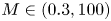 $M \in (0.3, 100)$ and
 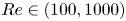 $Re \in (100, 1000)$, where the motion states are divided into steady, periodic, period-doubling, quasi-periodic and chaotic states which are determined by using the time history of wall motion trajectory, power spectral density (PSD), phase portrait and estimated dominant Lyapunov exponent. Here non-dimensional time of
  $t/T=400 - 1000$ is used for the nonlinear dynamics analysis, to exclude the influence from the initial transient behaviour. At
  $M=0.3$, only four cases are run as the simulations suffer from numerical instabilities for
  $Re>400$. Figure 9 demonstrates that the dynamic behaviours of the system are very complex. Specifically, the chaotic motion occurs mainly at high
  $Re$ and low mass ratios
  $M$ or low
  $Re$ and high mass ratios
  $M$. The continuity of the chaotic distribution is interrupted at
  $Re=250$,
  $M=6$ and
  $M=7$, which will be discussed in § 4.2.2. The steady motion occurs at low mass ratios (
 $M\le 3$). Taking the case of fixed mass ratio
  $M=1$ with varying
  $Re$ as an example, the system is steady at
  $Re=100$. An increase of the Reynolds number results in the loss of static equilibrium via supercritical Hopf bifurcation, leading to a periodic limit cycle oscillation at
  $Re=150$ and
  $Re=200$. For
  $250\le Re \le 500$, the system is steady. The system becomes chaotic at
  $Re=550$. However, a period-doubling state is observed at
  $Re=600$. The system reaches chaotic motion again via a quasi-periodicity route if the Reynolds number is further increased, similar to the Ruelle–Takens–Newhouse scenario (Ruelle & Takens Reference Ruelle and Takens1971; Newhouse et al. Reference Newhouse, Ruelle and Takens1978).

Figure 9. Motion state diagram in the  $Re-M$ parameter space with
  $K_s=2400$,
  $P_e=1.95$:
  $\boldsymbol {\Box }$, green - steady;
  $\boldsymbol {\vartriangle }$, blue - periodic;
  $\boldsymbol {\Diamond }$, yellow – period-doubling;
  $\boldsymbol {\bigcirc }$, orange – quasi-periodic;
  $\boldsymbol {\vartriangleright }$, red – chaotic.
At  $M=3$, the system is in a periodic state at
  $Re=100$ and then reaches a chaotic state at
  $Re=200$ via the period-doubling route. This process is similar to the classical Feigenbaum scenario (Feigenbaum Reference Feigenbaum1978, Reference Feigenbaum1979) of the route to chaos. For
  $6\le M \le 10$, most of the motion states switch back and forth between periodic and chaotic as
  $Re$ is increased. A similar phenomenon can also be observed for
  $650\le Re\le 1000$ as
  $M$ is increased. For high mass ratio at
  $M=50$ and
  $100$, only chaotic states are observed.
In order to discuss the flow physics associated with the states shown in figure 9, the transition process from steady to chaotic motion by fixing  $M=1$ and varying
  $Re$ is discussed in § 4.2.1 and that by fixing
  $Re=250$ and varying
  $M$ is presented in § 4.2.2.
4.2.1. Effects of $Re$

Here we first discuss  $M=1$,
  $Re=100$,
  $200$,
  $500$,
  $550$,
  $600$,
  $650$,
  $800$,
  $1000$,
  $2000$ and
  $3000$, and then discuss
  $M=10$,
  $Re=1000$,
  $2000$ and
  $3000$.
Figure 10 shows the  $y$-coordinate time history, the PSD and phase portrait consisting of the
  $y$-velocity vs
  $y$-coordinate of the mid-point of the upper collapsible channel wall for
  $M=1$ and different values of
  $Re$. Figure 11 displays the corresponding vorticity contours to discuss the physical mechanisms associated with these motion states.

Figure 10. The time history of the  $y$-coordinate of the mid-point (
 $x=2.5$ initially) at the upper elastic channel wall at various Reynolds numbers
  $Re$ with
  $M=1$,
  $K_s=2400$,
  $P_e=1.95$. Power spectral density and phase portrait in displacement-velocity (
 $y$–
$y$– $v$) space. The frequency in the PSD is normalized by
  $U_0/D$. Here
  $Re=100$: steady state;
  $Re=200$: periodic state;
  $Re=500$: steady state;
  $Re=550$: chaotic state;
  $Re=600$: period-doubling state;
  $Re=800$: chaotic state. Plot parameters: (a)
  $Re=100$: steady state; (b)
  $Re=100$: low energy; (c)
  $Re=100$: fixed point; (d)
  $Re=200$: periodic state; (e)
  $Re=200$: fundamental frequency
  $f_1$ and its harmonic frequencies,
  $2f_1$,
  $3f_1$; (f)
  $Re=200$: single limit cycle; (g)
  $Re=500$: steady state; (h)
  $Re=500$: low energy; (i)
  $Re=500$: fixed point; (j)
  $Re=550$: chaotic state; (k)
  $Re=550$: broadband continuous spectrum; (l)
  $Re=550$: chaotic attractor; (m)
  $Re=600$: period-doubling state; (n)
  $Re=600$: the arise of subharmonic frequencies
  $0.5f_1$,
  $1.5f_1$; (o)
  $Re=600$: multiple limit cycles; (p)
  $Re=650$: quasi-periodic state; (q)
  $Re=650$: the arise of second- and third fundamental frequencies,
  $f_2$,
  $f_3$; (r)
  $Re=650$: limit torus; (s)
  $Re=800$: chaotic state; (t)
  $Re=800$: broadband continuous spectrum; (u)
  $Re=800$: chaotic attractor.

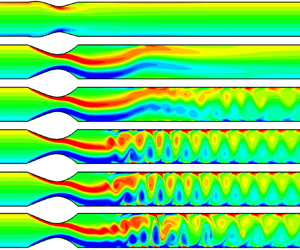
Figure 11. Instantaneous vorticity contours at  $t/T=100$ for various
  $Re$ with
  $M=1$,
  $K_s=2400$ and
  $P_e=1.95$. The vorticity ranges from
  $-10$ (blue) to 10 (red). Note: the aspect ratio (length/width) is set to
  $0.3$ for an overview of the whole flow field. Here
  $\textrm{A}(5, 0.5)$,
  $\textrm{B}(7, 0.5)$,
  $\textrm{C}(9, 0.5)$,
  $\textrm{D}(11, 0.5)$ and
  $\textrm{E}(13, 0.5)$ are five probe points. Animations of the vorticity contours for
  $Re=200$,
  $Re=550$,
  $Re=600$,
  $Re=650$ and
  $Re=800$ are provided in supplementary movies 1 to 5 available at https://doi.org/10.1017/jfm.2021.710.
At  $Re=100$ and
  $Re=500$, as shown in figures 10(a) and 10(g), the channel wall remains at its equilibrium position. A fixed point in the phase portrait (see figures 10c and 10i) indicates that the system is in a steady state at these
  $Re$. This is also revealed by a very low energy level of the PSD in figures 10(b) and 10(h). At
  $Re=200$, the time series in figure 10(d) displays periodic oscillations. In figures 10(e) and 10(f) the appearance of a fundamental frequency
  $f_1$ and its harmonics (i.e.
  $2f_1, 3f_1$ etc) and a single limit cycle in the phase portrait indicate that the system undergoes a period-1 limit cycle oscillation.
At  $Re=550$, the system experiences a chaotic motion, which is reflected by the broadband PSD in figure 10(k) and the chaotic attractor of the phase portrait in figure 10(l). Similar nonlinear dynamic characteristics can also be found at
  $Re=800$ in figures 10(t) and 10(u). Figures 10(j) and 10(s) show that the chaotic oscillations involve small non-repetitive noise-like fluctuations. To further examine the chaotic motion, the dominant Lyapunov exponents
  $\lambda$ are estimated by using the time-delay method of Wolf et al. (Reference Wolf, Swift, Swinney and Vastano1985). An open source MATLAB code (Wolf Reference Wolf2021) is used to calculate
  $\lambda$ based on a time series of
  $y$ velocity-displacement data. See Wolf et al. (Reference Wolf, Swift, Swinney and Vastano1985) for more details. This method has been adopted by Connell & Yue (Reference Connell and Yue2007) and Goza et al. (Reference Goza, Colonius and Sader2018) to identify the chaotic motion of flapping flags. Note that a zero or near-zero value of
  $\lambda$ corresponds to a non-chaotic motion state, while a positive value of
  $\lambda$ indicates a chaotic motion state, and a negative value of
  $\lambda$ represents a steady state. As the time-delay method of Wolf et al. (Reference Wolf, Swift, Swinney and Vastano1985) only allows the estimation of non-negative Lyapunov exponents, the dominant Lyapunov exponents for steady state are not estimated here. The time series of the
  $y$ velocity-displacement data is used in the phase space reconstruction. The computed results of
  $\lambda$ for
  $M=1$ at typical
  $Re$ values are shown in table 3. The estimated dominant Lyapunov exponents at
  $Re=550$ and
  $Re=800$ are
  $\lambda = 0.0385$ and
  $\lambda = 0.0417$, respectively. These relatively large positive values of
  $\lambda$ (
 $\sim$ of order
  $10^{-2}$) support that the motion type at
  $Re=550$ and
  $Re=800$ is chaotic.
Table 3. Estimated dominant Lyapunov exponents and corresponding motion states of the system:  $K_s=2400$,
  $P_e=1.95$. Here NA means not applicable as only the estimation of non-negative Lyapunov exponents are allowed for the time-delay method of Wolf et al. (Reference Wolf, Swift, Swinney and Vastano1985).

At  $Re=600$, the appearance of a subharmonic frequency
  $0.5f_1$ in the PSD (see figure 10n) and multiple limit cycles in the phase space (see figure 10o) indicate that the system experiences a period-doubling bifurcation. Figure 10(m) shows the regular oscillations for the period-doubling motion state. When the Reynolds number is further increased to
  $Re=650$, a quasi-periodic motion state is identified, which is confirmed by the appearance of second- and third-fundamental frequencies (i.e. incommensurate frequencies
  $f_2$ and
  $f_3$,
  $f_2/f_1$ and
  $f_3/f_1$ are irrational) in the PSD of figure 10(q) and the limit torus in the phase space of figure 10(r).
With the introduction of two new incommensurate frequencies, the multiple limit cycles at  $Re=600$ turn into a dense toroidal structure (see figure 10r). Figure 10(p) shows the quasi-periodic oscillations of the mid-point of the upper elastic channel wall at
  $Re=650$.
From figure 11, it is found that the elastic channel walls bulge outward at  $Re=100$. At
  $Re=200$, the walls undergo a mode-2 shaped deformation (i.e. with two half-wavelengths along the elastic wall). The walls indent inward of the channel with a further increase of
  $Re$. Whether the collapsible walls bulge outward or indent inward is determined by the resultant force acting on the elastic walls, which consists of the external pressure
  $P_e$ and the fluid stress. The normal component of the external force is the transmural pressure
  $p-P_e$ (i.e. internal minus external pressure), which is affected by the pressure loss in the channel. As seen from figure 12, the pressure inside the channel is large at
  $Re=100$ due to higher pressure loss, so that a positive transmural pressure (i.e.
  $p-P_e>0$) is developed and pushes the elastic walls outward. For
  $Re > 200$, the pressure inside the channel is small enough as the pressure loss becomes smaller, so that a negative transmural pressure (
 $p-P_e<0$) causes the elastic walls to move inward. This phenomenon is consistent with the finding of Luo et al. (Reference Luo, Cai, Li and Pedley2008) that the wall curvature is determined by the transmural pressure.

Figure 12. The transmural pressure distributions along the upper elastic channel walls for different  $Re$ with
  $M=1$,
  $K_s=2400$ and
  $P_e=1.95$.
In addition, the physical mechanisms that lead to the different motion states are varied. For  $Re=100$, the viscosity is strong enough to damp out any small disturbance. The very positive transmural pressure (i.e.
  $p-P_e \sim 2$) along the whole elastic channel walls and the relatively small wall inertia (i.e.
  $M=1$) lead to a steady state at
  $Re=100$. The transmural pressure decreases as the Reynolds number increases. At
  $Re=200$, the configuration of the elastic walls contains two half-wavelengths. The system is unstable to this mode
  $2$ perturbation due to a mode 2 transmural pressure distribution formed where a positive transmural pressure at the anterior segment of the collapsible walls (i.e.
  $x\leq 1$) pushes the walls outward and a negative transmural pressure at the remaining part of the collapsible walls (i.e.
  $1< x\leq 5$) causes the walls to move inward. As a result, this unbalanced transmural pressure along the collapsible walls causes the self-excited oscillations of the walls. The self-excited oscillations at
  $Re=200$ can be explained as follows which has been recognized as one of the main mechanisms for the oscillations of collapsible tubes (Luo et al. Reference Luo, Cai, Li and Pedley2008). The flow accelerates to higher speed at the downstream end of the elastic walls as the channel becomes more constricted. Then the pressure decreases due to conservation of mass, which enhances the constriction further. This in turn causes the increase of viscous resistance in the vicinity of the constriction, either through viscous dissipation in the boundary layers, or through flow separation. As a result, upstream pressure will rise due to a higher pressure drop required to maintain the flow rate, causing the upstream half of the elastic walls to bulge out further, and then forcing the reopening of the constriction. At
  $Re=500$, a very negative transmural pressure is observed in figure 12, which causes the channel walls to collapse and indent inward. Furthermore, as shown in figure 11, at
  $Re=500$, flow separation occurs slightly downstream of the narrowest point, and a stable but asymmetric jet is developed with the jet attaching to the lower wall. Owing to the Coanda effect, such asymmetry can be maintained, resulting in an increase in the velocity and a decrease in the pressure near the lower wall. The very negative transmural pressure, a stable jet flow without vortex shedding and the weak effect of the wall inertia lead to a steady configuration at
  $Re=500$. The flow becomes unsteady if the Reynolds number further increases. As seen in figure 11, at
  $Re=550$, the jet flow between the recirculation zones loses its stability and breaks into small vortices that are transported downstream. Then the flow becomes time dependent, and the channel walls enter a chaotic motion state.
At  $Re=600$, figure 11 shows that there is vortex shedding downstream of the throat. To trace the PSD of the streamwise velocity, five probe points (i.e.
  $\textrm{A}(5, 0.5)$,
  $\textrm{B}(7, 0.5)$,
  $\textrm{C}(9, 0.5)$,
  $\textrm{D}(11, 0.5)$ and
  $\textrm{E}(13, 0.5)$ as shown in figure 11 at
  $Re=600$) are monitored. Figure 13 shows that the streamwise velocities at five probe points are all in period-doubling oscillations as indicated by the subharmonic frequencies
  $0.5f_1$ and
  $1.5f_1$ in the PSD. The periodic component is attributed to the periodic shedding of vortices downstream of the throat that feeds back periodic perturbations on the elastic walls. The partial pairing of two adjacent vortices (as marked in figure 11) downstream of the elastic walls further feeds back subharmonic perturbations on the elastic walls that trigger period-doubling oscillations of the elastic walls. This process is further demonstrated by supplementary movie 3. A similar vortex pairing process can be found in the coherent structure interactions in a mixing layer (Hussain Reference Hussain1986) and in the vortex shedding in an arterial stenosis (Bluestein et al. Reference Bluestein, Gutierrez, Londono and Schoephoerster1999). Results in figure 13 show that the PSD of the subharmonic frequency
  $0.5f_1$ increases in the streamwise direction and reaches its peak value at
  $\textrm{D}(11, 0.5)$ indicating that a partial pairing process occurs between
  $\textrm{C}(9, 0.5)$ and
  $\textrm{D}(11, 0.5)$, which further supports the conclusion that the period-doubling oscillations at
  $Re=600$ are caused by the periodic vortex shedding and the partial pairing of two adjacent vortices.

Figure 13. The PSD of the streamwise velocity  $u$ at five probe points:
  $\textrm{A}(5, 0.5)$,
  $\textrm{B}(7, 0.5)$,
  $\textrm{C}(9, 0.5)$,
  $\textrm{D}(11, 0.5)$ and
  $\textrm{E}(13, 0.5)$ for
  $Re=600$.
As the Reynolds number is further increased to  $Re=650$, periodic vortex shedding downstream of the throat is also observed. Apart from that, there is a merging of adjacent three vortices at
  $x\approx 10$ (as marked in figure 11) that feeds back additional perturbations on the elastic walls leading to quasi-periodic oscillations in the channel walls. The merging process is further demonstrated by supplementary movie 4.
At  $Re=800$, the vortex merging at
  $x\approx 10$ and the interactions between the vortices on the upper and lower walls downstream at
  $x\approx 14$ cause the walls to settle into chaotic oscillations featuring small noise-like fluctuations as shown in supplementary movie 5. Further simulations have been conducted for a single-sided collapsible channel. There is no vortex shedding downstream of the throat due to mild stenoses (e.g.
  $28\,\%$ diameter reduction at
  $Re=1000$) formed with only one collapsed wall. Therefore, the system is steady for
  $Re>300$, and the period-doubling, quasi-periodic and chaotic motion states caused by the interactions between the collapsed wall and the vortices are not observed.
The motion of flexible walls is chaotic at high Reynolds number for mass ratios of 1 and 10 between which there are periodic and period-doubling states. In order to compare the chaotic behaviours at high Reynolds numbers at different mass ratios, two mass ratios ( $M=1$ and
  $10$) are considered at
  $K_s=2400$,
  $P_e=1.95$ and
  $Re=1000$,
  $2000$ and
  $3000$. Figure 14 shows the time history of the
  $y$-coordinate of the mid-point (
 $x=2.5$ initially) of the upper and lower elastic walls. For
  $M=1$ and
  $Re=1000$, as seen in figure 14(a), there is no obvious oscillation of the elastic walls after collapse. When the mass ratio increases to
  $M=10$, the elastic walls gradually start to develop self-excited oscillations after collapse (see figure 14b). When the Reynolds number increases to
  $Re=2000$ for
  $M=1$, the elastic walls experience irregular small-amplitude oscillations (approximately
  $0.02D$ as shown in figure 14c), and such oscillations are more evident and irregular at
  $Re=3000$ (see figure 14e). Figures 14(d) and 14(f) show that, for
  $M=10$ at
  $Re=2000$ and
  $Re=3000$, the elastic walls undergo much larger-amplitude oscillations (approximately
  $0.1D$) because of the higher inertia.

Figure 14. The  $y$-coordinate time history of the mid-point (
 $x=2.5$ initially) at the collapsible channel walls at various Reynolds numbers
  $Re$ with
  $M=1$ and
  $M=10$. Other dimensionless parameters are
  $K_s=2400$,
  $P_e=1.95$. The red line and blue line represent the
  $y$-coordinate of the upper and lower elastic wall, respectively. Plot parameters: (a)
  $M=1$,
  $Re=1000$; (b)
  $M=10$,
  $Re=1000$; (c)
  $M=1$,
  $Re=2000$; (d)
  $M=10$,
  $Re=2000$; (e)
  $M=1$,
  $Re=3000$; (f)
  $M=10$,
  $Re=3000$.
Instantaneous vorticity contours for various  $Re$ at
  $M=1$ and
  $M=10$ are presented in figure 15. Overall, the diffusion of vortices decreases with the increase of Reynolds number due to the reduced viscosity. As a result, stronger vortices and thinner boundary layers are observed as the Reynolds number increases. As seen from figure 15(a) for
  $M=1$, a streaming jet flow attaches to the lower wall at
  $Re=1000$. The jet flow between the recirculation zones loses its stability and breaks up into small vortices that are transported downstream. At
  $Re=2000$, the region of shed vortices is closer to the upstream end of the elastic walls when compared with
  $Re=1000$. Moreover, for
  $x\geq 10$ at
  $Re=2000$, a clear reverse Kármán vortex street (indication of a jet flow) is observed with two staggered rows of vortices being transported downstream. The vortices are counterclockwise (positive vorticity) in the upper row and clockwise (negative vorticity) in the lower row. It is interesting to note that the instantaneous vorticity contours at
  $Re=3000$ show two non-staggered rows of vortex street right at the end of the elastic walls, but they lose stability and interact with each other from
  $x=8$. In addition, the system loses stability at
  $Re=2000$ and
  $Re=3000$, and the elastic walls move up and down alternately, generating vorticity waves downstream. Such instability at
  $Re=2000$ and
  $Re=3000$ can also be explained by the shear layer instabilities as demonstrated in § 4.2.1. As can be seen from figure 15(a), at
  $M=1$ and
  $Re=1000$, the shed vortices are far downstream from the elastic walls and, thus, have a weak impact on their motion. However, at
  $Re\geq 2000$, the shed vortices, which are close to the mid-point of the elastic walls, feeds back perturbations on the elastic walls to produce small-amplitude self-excited oscillations in the elastic walls.

Figure 15. Instantaneous vorticity contours under different  $Re$ at
  $t/T=200$ with
  $M=1$ and
  $M=10$,
  $K_s=2400$ and
  $P_e=1.95$. The vorticity ranges from
  $-10$ (blue) to 10 (red). Note: the aspect ratio (length/width) is set to
  $0.3$ for an overview of the whole flow field. Plot parameters: (a)
  $M=1$ with
  $Re=1000$,
  $2000$ and
  $Re=3000$; (b)
  $M=10$ with
  $Re=1000$,
  $2000$ and
  $3000$.
From the above analysis, it is found that the vortex shedding caused by shear layer instabilities at  $Re=2000$ and
  $Re=3000$ are responsible for the onset of self-excited oscillations. As seen from figure 15(b) for
  $M=10$, at
  $Re=1000$, a series of vortex pairs dissipating quickly downstream are observed, while an asymmetric jet flow is observed at
  $M=1$. The higher amplitude of the self-excited oscillations at
  $M=10$ than at
  $M=1$ indicates stronger FSIs between the jet and the elastic walls at the higher mass ratio. In this situation, the whole of the elastic walls undergo large-amplitude oscillations (see figure 15(b) at
  $Re=1000$ and
  $M=10$). The oscillations become regular at
  $Re=1000$ when the mass ratio increases from
  $M=1$ to
  $M=10$ (see figure 14).
For  $M=10$, the large-amplitude and irregular oscillations at
  $Re=2000$ and
  $Re=3000$ are the results of interactions between different instability modes (i.e. the instabilities induced by the shedding of vortices at high
  $Re$ and the travelling-wave flutter induced by the wall elasticity at high
  $M$).
$M$).
4.2.2. Effects of $M$

At  $Re=250$, there are no vorticity waves convecting downstream of the elastic walls when
  $M$ varies from
  $1$ to
  $8$. Therefore, the wall inertia plays an important role in inducing the different motion states of the elastic walls. Six cases (
 $M=1$,
  $4$,
$4$,  $5$,
$5$,  $6$,
$6$,  $7$ and
  $8$) are analysed in detail. Figure 16 shows the corresponding
  $y$-coordinate time history, the PSD and phase portrait of
  $y$-velocity vs
  $y$-coordinate of the mid-point at the upper collapsible wall. The travelling-wave flutter of
  $M=5$ is shown in figure 17. Figure 18 displays the corresponding instantaneous vorticity contours of the flow field.

Figure 16. The time history of the  $y$-coordinate of the mid-point (
 $x=2.5$ initially) of the upper elastic wall under different mass ratios
  $M$ with
  $Re=250$,
  $K_s=2400$,
  $P_e=1.95$. Power spectrum density (PSD) and phase portrait in displacement-velocity (y-v) space. The frequency in the PSD is normalized by
  $U_0/D$. Here
  $M=1$: steady state;
  $M=4$: periodic state;
  $M=5$: period-doubling state;
  $M=6$: periodic state;
  $M=7$: quasi-periodic state;
  $M=8$: chaotic state. Plot parameters: (a)
  $M=1$: steady state; (b)
  $M=1$: low energy; (c)
  $M=1$: fixed point; (d)
  $M=4$: periodic state; (e)
  $M=4$: fundamental frequency
  $f_1$ and its harmonic frequencies
  $2f_1$,
  $3f_1$; (f)
  $M=4$: limit cycle; (g)
  $M=5$: period-doubling state; (h)
  $M=5$: the arise of subharmonic frequencies
  $0.5f_1$,
  $1.5f_1$; (i)
  $M=5$: multiple limit cycles; (j)
  $M=6$: periodic state; (k)
  $M=6$: fundamental frequency
  $f_1$ and its harmonic frequencies
  $2f_1$,
  $3f_1$; (l)
  $M=6$: limit cycle; (m)
  $M=7$: quasi-periodic state; (n)
  $M=7$: the arise of second- and third fundamental frequencies,
  $f_2$,
  $f_3$; (o)
  $M=7$: limit torus; (p)
  $M=8$: chaotic state; (q)
  $M=8$: broadband continuous spectrum; (r)
  $M=8$: chaotic attractor.

Figure 17. Travelling-wave flutter at  $Re=250$,
  $M=5$,
  $P_e=1.95$ and
  $K_s=2400$: (a) the time histories of pressure and
  $y$-coordinate for the mid-point (
 $x=2.5$ initially) on the upper elastic wall; (b) the spatial wave of the wall shapes at four different instants shown in (a). (a) The
  $p$ and
  $y$-coordinate time histories, (b) wall shapes.

Figure 18. Instantaneous vorticity contours under different mass ratios at  $t/T=100$ with
  $Re=250$,
  $K_s=2400$ and
  $P_e=1.95$. The vorticity ranges from
  $-10$ (blue) to 10 (red). Note: the aspect ratio (length/width) is set to
  $0.3$ for an overview of the whole flow field. Animations of the vorticity contours for
  $M=5 - 8$ are provided in supplementary movies 6 to 9.
Similar to  $Re=200$ and
  $M=1$ in figure 10, a steady motion is observed at
  $Re=250$ and
  $M=1$, as demonstrated by the wall remaining at its equilibrium position in figure 16(a), the low energy level in figure 16(b) and the fixed point in the phase portrait shown in figure 16(c). When
  $M$ increases to
  $4$, the wall motion is periodic (see figure 16d) with a fundamental frequency
  $f_1$ and its harmonics (i.e.
  $2f_1$,
  $3f_1$ etc) (see figure 16e). This is supported by the limit cycle in figure 16(f). When the mass ratio increases to
  $M=5$, the system settles into a period-doubling state, which is confirmed by the appearance of subharmonic frequencies
  $0.5f_1$ and
  $1.5f_1$ in figure 16(h) and multiple limit cycles in figure 16(i). Figure 16(g) shows the corresponding motion state. At
  $M=6$, the system experiences a period-1 limit cycle oscillation, as demonstrated by the periodic oscillations in figure 16(j), the PSD in figure 16(k) and a single limit cycle in figure 16(l). The system then enters a quasi-periodic motion at
  $M=7$ as evidenced by the quasi-periodic wave shapes in figure 16(m), the PSD in figure 16(n) and the limit torus in figure 16(o). At
  $M=8$, the broadband continuous spectrum in figure 16(q) and the chaotic attractor in figure 16(r) indicate that the system enters a chaotic motion. The estimated dominant Lyapunov exponents
  $\lambda$ for these cases listed in table 4, support the identification of chaotic motion at
  $M=8$ (
 $\lambda =0.5705$ (
 $\sim$ of order
  $10^{-1}$)). Figure 16(p) shows that the corresponding chaotic motion involves non-repetitive irregular oscillations, which is quite different from the chaotic oscillations observed in figures 10(j) and 10(s) where the dynamic behaviours of the elastic walls feature small noise-like fluctuations.
Table 4. Estimated dominant Lyapunov exponent and corresponding motion state of the system:  $K_s=2400$,
  $P_e=1.95$. Here NA means not applicable.

The changes in behaviour with the increase of mass ratio are now explored by analysing the vortex structures shown in figure 18. Compared with the vortex structure in figure 11, the vortices in figure 18 are more apparent in the collapsible section of the channel compared with other regions. This difference is caused by the effects of Reynolds number. In figure 11 the Reynolds number for most cases are  $Re\geq 500$, which causes a longer jet flow between the recirculation zones. Therefore, the vortices are less apparent in the collapsible section of the channel. As for the vortices in figure 18, a shorter jet flow is formed due to the low Reynolds number (
 $Re=250$), leading to more apparent vortices in the collapsible section. At
  $Re=250$, a negative transmural pressure causes the channel walls to indent inward. The relatively weak wall inertia at
  $M=1$ enables the system to be steady with the formation of a stable jet flow. As the mass ratio increases to
  $M=4$, the relatively heavy elastic walls periodically produce a jet flow, independent of the generation of vorticity waves downstream. This result indicates that the periodic oscillations of the elastic walls can be induced by increasing the wall inertia. The flow and wall shapes are still symmetric, indicating that symmetry breaking is not necessary for the onset of self-excited oscillations.
The effect of wall inertia becomes more evident at  $M=5$ with a pair of small vortices shedding downstream of the elastic walls. Due to the relatively strong diffusion of vortices at
  $Re=250$, these vortices dissipate quickly. Figure 17(a) shows the time histories of pressure and
  $y$-coordinate for the mid-point on the upper elastic wall. The oscillations of the wall
  $y$-coordinate and wall pressure are slightly out of phase, indicating that energy has been irreversibly transferred to the elastic walls, leading to flutter of the walls. Figure 17(b) shows the spatial wave of the wall shapes at four instants shown in figure 17(a). The wall has one wave at
  $t1$ and
  $t2$, moving to two waves at
  $t3$ and
  $t4$ which implies that travelling-wave flutter is formed at
  $M=5$. The travelling-wave flutter has also been found by Luo & Pedley (Reference Luo and Pedley1998) for a one-sided collapsible channel flow. The period-doubling oscillations at
  $M=5$ are caused by the travelling-wave flutter along the elastic walls (see supplementary movie 6 for an animation of the vorticity contours). At
  $M=6$, a period-1 limit cycle oscillation has been induced by the wall inertia. The flow is still symmetric until the symmetry breaking of the collapsible channel walls at
  $M=8$. The chaotic oscillations at
  $M=8$ (heavy walls) are due to symmetry breaking coupled with the travelling-wave oscillation along the elastic walls induced by the wall elasticity (see supplementary movie 9 for an animation of the vorticity contours). This scenario shows some similarity to the aeroelastic flutter of a bridge. For fixed
  $Re=250$ with varying
  $M$, the mass ratio is the major parameter that causes symmetry breaking of the collapsible channel flow. Therefore, the mass ratio controls the onset of chaos, which will arise once this parameter becomes sufficiently high. A similar observation was reported by Connell & Yue (Reference Connell and Yue2007) for a 2-D flapping flag in a uniform flow.
Here the effects of a wider range of mass ratios are examined:  $M=0.3$,
  $1$,
$1$,  $2$,
$2$,  $5$,
$5$,  $10$ and
  $20$ while the other non-dimensional governing parameters are fixed as follows:
  $Re=500$,
  $K_s=2400$ and
  $P_e=1.95$. Figure 19 shows the time history of the
  $y$-coordinate of the mid-point of the elastic walls for different mass ratios. The oscillation amplitude of the elastic walls increases with the mass ratio
  $M$, with solutions that are steady for
  $M\leq 0.3$ (see figure 19(a), results of
  $M=0.1$ and
  $M=0.2$ not shown here). For
  $M=1$, as shown in figure 19(b), the startup transient oscillation decays with time and the system reaches steady state at
  $t/T=80$. When
  $M$ is relatively small (e.g.
  $M\leq 2$), the oscillation amplitude is less than 0.01 (see figure 19c) but increases significantly for
  $M\geq 10$, as shown in figures 19(d) and 19(e), changing from small-amplitude mode at
  $M=5$ to large-amplitude mode at
  $M=10$. These results indicate that the self-excited oscillations of the elastic walls are closely related to the mass ratio of the wall.

Figure 19. The time history of the  $y$-coordinate for the mid-point (
 $x=2.5$ initially) on the elastic walls for different mass ratios
  $M$ with
  $Re=500$,
  $K_s=2400$,
  $P_e=1.95$. The red line and blue line represent the upper and lower elastic wall, respectively. Plot parameters: (a)
  $M=0.3$; (b)
  $M=1$; (c)
  $M=2$; (d)
  $M=5$; (e)
  $M=10$; (f)
  $M=20$.
Figure 19(f) shows an interesting oscillation mode at  $M=20$. Following the collapse of the elastic walls initially (from
  $t/T=0$ to
  $t/T=17$), the oscillation grows and settles into large amplitude. We examine one specific cycle in figures 20 and 21. Figure 20(a) shows the time history of the
  $y$-coordinate and figure 20(b) shows the corresponding wall shapes at six instants, as indicated in figure 20(a). It is seen from figure 20(b) that the deformations of the two elastic walls are always symmetric at
  $t1$ to
  $t6$. The walls bulge out strongly upstream at
  $t1$ then bounce back to a strongly collapsed state at
  $t4$.
$t4$.

Figure 20. The  $y$-coordinate time history for the mid-point (
 $x=2.5$ initially) on the upper elastic wall (a) and the wall shapes (b) corresponding to the six instants shown in (a) for
  $M=20$ with
  $Re=500$,
  $K_s=2400$,
  $P_e=1.95$. (a) The
  $y$-coordinate time history. (b) Wall shapes.

Figure 21. Instantaneous vorticity contours at six instants marked in figure 20(a) for  $M=20$,
  $Re=500$,
  $K_s=2400$,
  $P_e=1.95$. The vorticity ranges from
  $-7$ (blue) to
  $7$ (red).
In figure 21 the corresponding vorticity contours clearly show the vortex pair evolution, migration and dissipation process. The vortices are always symmetric even at this high wall inertia ( $M=20$). More specifically, a pair of vortices
  $p1$ is shed downstream of the elastic walls at
  $t1$ and is convected downstream accompanied with the collapse of the walls. A new vortex pair
  $p2$ is generated at
  $t2$ and is convected downstream with the further collapse of the elastic walls at
  $t3$. At
  $t4$ when the elastic walls reach to their most collapsed state, a strong central jet emerges and entrains the surrounding fluid including the vortices. After reopening of the collapsed channel, the former vortex pairs (i.e.
  $p1$ and
  $p2$) are convected further downstream (
 $t5$) and a new vortex pair
  $p3$ is shed again beyond the throat (
 $t6$). Such a fluid flow is different from the jet produced in a nozzle and shows some similarity to the jet propulsion of a cephalopod under water (Luo et al. Reference Luo, Xiao, Zhu and Pan2020).
4.3. Effects of external pressure $P_e$ at $Re=500$


Here the effects of external pressure  $P_e$ (
 $=1$,
$=1$,  $2$,
$2$,  $3$,
$3$,  $5$,
$5$,  $8$ and
  $10$) exerted on the elastic walls are further investigated, while the other non-dimensional governing parameters are fixed at
  $Re=500$,
  $K_s=2400$ and
  $M=1$.
Figure 22 shows the time history of the  $y$-coordinate of the mid-point on the elastic walls. Overall, it is seen that self-excited oscillations occur under large external pressure (for
  $P_e \ge 5$, see figures 22d, 22e and 22f) and the oscillation amplitude increases with
  $P_e$. Specifically, as shown in figure 22(a) (
 $P_e=1$), the walls reach a stable state immediately after collapse. For
  $P_e=2$ and
  $P_e=3$ (see figures 22b and 22c), the elastic walls experience small-amplitude oscillations, but the walls reach a steady state as the oscillations decay with time. At
  $P_e=5$ and
  $P_e=8$, small-amplitude (less than
  $0.01D$) self-excited oscillations are developed. As shown in figure 22(f), at
  $P_e=10$, high-frequency small-amplitude self-excited oscillations are superimposed on low-frequency large-amplitude oscillations. These results indicate that
  $P_e$ triggers the onset of self-excited oscillations and controls their amplitude.

Figure 22. The time history of the  $y$-coordinate of the mid-point (
 $x=2.5$ initially) of the elastic walls under different external pressures
  $P_e$ with
  $Re=500$,
  $K_s=2400$,
  $M=1$. The red line and blue line represent the upper and lower elastic wall, respectively. Plot parameters: (a)
  $P_e=1$; (b)
  $P_e=2$; (c)
  $P_e=3$; (d)
  $P_e=5$; (e)
  $P_e=8$; (f)
  $P_e=10$.
We examine the special oscillation mode at  $P_e=10$. Figure 23 shows the time history of the
  $y$-coordinate of the mid-point at the upper elastic wall, and the vorticity contours at the seven instants marked in figure 23 are shown in figure 24. Figure 23 shows that the oscillations at
  $P_e=10$ are highly irregular, which is in a chaotic motion state. It can be seen from figure 24 that the motions of the upper and lower elastic walls are asymmetric with complex vortex structures, in contrast to the symmetric vortex structures shown in figure 21. From
  $t1$ to
  $t4$, initially, the opposite elastic walls approach each other, reducing the cross-section area of the channel. The fluid reaches the maximum speed at the throat of the channel, reducing the pressure, which causes a further collapse of the channel until the channel is almost closed at
  $t5$. From
  $t1$ to
  $t4$, the vortices are convected downstream quickly until
  $t5$ when the vortices stop convecting downstream further until the channel reopens at
  $t6$. The kinetic energy of the upstream fluid is converted to a pressure increase that causes the channel to reopen at
  $t6$, and the cycle is repeated.

Figure 23. The time history of the  $y$-coordinate for the mid-point (
 $x=2.5$ initially) on the upper elastic wall with
  $M=1$,
  $P_e=10$,
  $Re=500$ and
  $K_s=2400$.

Figure 24. Instantaneous vorticity contours at seven instants during large-amplitude self-excited oscillations for  $M=1$,
  $P_e=10$,
  $Re=500$ and
  $K_s=2400$. The vorticity ranges from
  $-10$ (blue) to 10 (red).
4.4. Discussion
A two-sided collapsible channel flow is numerically studied here. An IB-LBM FSI strategy is extended to model the FSI system. Compared with the conventional ALE, the IB-LBM FSI algorithm is simple because the Cartesian mesh is used and mesh movement is avoided. Further, the advantages of explicit calculation and the intrinsic parallel nature of LBM make the IB-LBM FSI solver much more efficient (up to 100 times) than the conventional ALE FSI solver in terms of computation time (Luo et al. Reference Luo, Cai, Li and Pedley2008). In addition, previously unexplored regions of the parameter space, such as high Reynolds number ( $Re$ up to 3000), high structure-to-fluid mass ratio (maximum
  $M=100$) and high external pressure (maximum
  $P_e=10$) are further examined here.
4.4.1. The role of symmetry breaking
Results here show that the symmetry breaking of the collapsible channel flow system may be induced by the increase of Reynolds number, wall inertia (mass ratio) and external pressure applied on the collapsible channel walls. Symmetry breaking is not a prerequisite for self-excited oscillations, but the symmetry breaking of the dynamic response of the elastic walls leads to the chaotic motion of this system.
Firstly, at low mass ratio  $M=1$, the symmetry breaking arises at the Reynolds number of
  $Re=320$ owing to a pitchfork bifurcation. The flow is steady both before and after the symmetry breaking bifurcation. A similar observation of such flow asymmetry has been reported by Kounanis & Mathioulakis (Reference Kounanis and Mathioulakis1999) in the experimental study of flow within a self-oscillating collapsible tube. They further reported that the flexible tube started oscillating when flow asymmetry occurred, while there are no oscillations in the collapsible walls here when flow asymmetry first appears. Kounanis & Mathioulakis (Reference Kounanis and Mathioulakis1999) pointed out that the symmetry breaking of the flow downstream of the collapsible segment may be a potential mechanism for the onset of self-excited oscillations. The different observations from this study are due to the much higher stretching stiffness and the negative transmural pressure (instead of a low and positive transmural pressure) here as well as the geometric difference (i.e. two dimensional in our model and three dimensional in Kounanis & Mathioulakis Reference Kounanis and Mathioulakis1999). The flow bifurcation investigated in § 4.1 shows that the occurrence of symmetry breaking of the jet flow at
  $Re=320$ and
  $M=1$ does not excite any oscillation of the elastic walls. In contrast, the collapsible channel flow system is still symmetric with periodic oscillations of the elastic walls at
  $Re=250$ and
  $M=2$ in § 4.2.2. Therefore, with regard to the role of symmetry breaking in the instability of a collapsible flow system, the different dynamic behaviours at
  $Re=320$ for
  $M=1$ and
  $Re=250$ for
  $M=2$ indicate that the symmetry breaking is not a prerequisite for the onset of self-excited oscillations.
Secondly, as shown in § 4.2.2, for  $Re=250$, the collapsible channel flow is symmetric for
  $M\leq 7$, and the symmetry breaking of the collapsible channel walls occurs at
  $M=8$, where the system settles into a chaotic state. Finally, as shown in figures 22 and 23, for
  $M=1$, the symmetry breaking occurs at
  $P_e=10$ where the system settles into a chaotic state again. These observations indicate that the symmetry breaking induced by the wall inertia and the external pressure can lead the collapsible system into a chaotic state.
4.4.2. Chaotic channel wall motions
The existence of chaotic motion is confirmed by a positive dominant Lyapunov exponent ( $\ge 10^{-2}$) and a chaotic attractor in the phase portrait of the
  $y$ velocity displacement of the mid-point at the collapsible channel walls. Aperiodic oscillations were observed experimentally by Bertram et al. (Reference Bertram, Raymond and Pedley1991) for
  $Re>4400$ in a thick-walled silicone rubber tube. The presence of chaos cannot be certainly confirmed due to the limited time recordings made in their experiments. Results in § 4.2 show that chaos can occur over a wide range of Reynolds numbers (i.e.
  $100\leq Re\leq 1000$), predominantly for high Reynolds numbers at low mass ratios (i.e.
  $Re\geq 500$ and
  $M \leq 4$); and for low Reynolds numbers with high mass ratios (i.e.
  $Re\leq 300$ and
  $M \geq 6$). Furthermore, in a general investigation of the routes to chaos for this system, two possibilities are found: the system reaches chaos via period-doubling or quasi-periodic bifurcations. The routes to chaos in the collapsible system have not been reported previously.
4.4.3. Rich dynamic behaviours
The dynamic behaviours of the collapsible system are qualitatively categorized into four major groups. The first group involves periodic oscillations of single fundamental frequency  $f_1$. The second group involves period-doubling oscillations of one fundamental frequency
  $f_1$ and its subharmonic frequencies
  $0.5f_1$ and
  $1.5f_1$. These period-doubling oscillations show two different wave shapes (e.g. figure 10m and 16g). The third group, as is shown in figure 10(p), involves quasi-periodic oscillations of three incommensurate frequencies (i.e.
  $f_1$,
  $f_2$ and
  $f_3$). The last group involves chaotic oscillations including small noise-like fluctuations (e.g. figures 10j and 10s) and non-repetitive irregular oscillations (e.g. figure 16p). Similar oscillation types were also observed by Bertram et al. (Reference Bertram, Raymond and Pedley1990) in the experimental study of collapsed tubes, where the experimentally observed oscillation types were categorized into six major groups including highly nonlinear periodic oscillations of relatively low frequency with two groups of different wave shapes, intermediate-frequency oscillations (nonlinear periodic oscillations at two or three times the frequency), high-frequency oscillations, smaller non-repetitive noise-like fluctuations and very-high-frequency oscillations. Irregular oscillations were also observed in their experiments as a genuine part of the dynamical behaviours of the collapsible system rather than due to any lack of control of experimental conditions.
4.4.4. Physical mechanisms responsible for the onset of self-excited oscillations
A wide range of the controlled parameters of the collapsible channel flows are investigated in this study ( $100 \leq Re \leq 3000$,
  $0.3\leq M \leq$
  $100$ and
  $1\leq P_e \leq 10$), and rich dynamic behaviours of the collapsible system are observed. The physical mechanisms responsible for the onset of these different oscillations are different, depending on the controlled parameters, and are summarized as follows.
(i) Unbalanced transmural pressure. In the investigation of the effects of Reynolds number shown in § 4.2.1, for
$Re\leq 500$, $M\leq 1$, $P_e=1.95$ and $K_s=2400$, there is no vortex shedding downstream of the elastic walls and the stability of the collapsible channel walls are mainly determined by the transmural pressure. Under these parameter conditions, the viscosity is strong enough to damp out any small disturbances caused by wall inertia. The only unstable source, take $Re=200$ as an example, comes from the unbalanced transmural pressure (positive upstream and negative downstream) along the elastic walls that causes self-excited oscillations. Either positive transmural pressure ($Re=100$) or negative transmural pressure ($250\leq Re\leq 500$) along the elastic walls can produce a steady state. Luo et al. (Reference Luo, Cai, Li and Pedley2008) demonstrated that the transmural pressure could affect the stability of the collapsible system through its interaction with the wall curvature, which supports our findings here.(ii) Shear layer instabilities. As the Reynolds number increases, it is found that the generation and shedding of vortices play a major role in the stability of the collapsible system. The shedding of vortices downstream of the throat feeds back perturbations on the elastic walls. For
$M\leq 1$, the instabilities in the wall motion for $550\leq Re\leq 3000$ are mainly due to shear layer instabilities. Luo & Pedley (Reference Luo and Pedley1996) firstly showed in a coupled FSI of a one-sided collapsible channel that the oscillations are a consequence of the generation of vorticity waves downstream. The effects of $Re$ in § 4.2.1 reveal that the vortex shedding downstream of the throat are responsible for the onset of self-excited oscillations. Furthermore, the period-doubling, quasi-periodic and chaotic oscillations are closely associated with vortex pairing and merging of adjacent vortices, and the interactions between vortices on the upper and lower walls.(iii) Wall elasticity at large mass ratios. For the onset of chaotic oscillations at
$Re=250$ and $M=8$ in § 4.2.2, travelling-wave flutter along the elastic walls induced by the wall elasticity causes the symmetry breaking that further triggers chaotic oscillations. For high Reynolds numbers at high mass ratios, as shown in figure 14, the travelling-wave flutter induced by the wall elasticity at high mass ratios (e.g. $M=10$) increases the oscillation amplitude approximately by a factor of five (e.g. from $0.02D$ at $M=1$ and $Re=2000$ to $0.1D$ at $M=10$ and $Re=2000$). The numerical study of the effects of wall inertia on a one-sided collapsible channel flow of Luo & Pedley (Reference Luo and Pedley1998) is the first study where collapse and flutter were examined together. They focused on low mass ratios ($M\leq 1$) as otherwise the amplitude of the oscillations became too large for the mesh generator to manage. As was observed by Luo & Pedley (Reference Luo and Pedley1998), the flutter observed here is not a consequence of the generation of vorticity waves downstream. The flutter found in Luo & Pedley (Reference Luo and Pedley1998) was caused by a phase difference between the wall pressure and wall displacement, which enables the fluid to transfer energy continuously to the wall. The flutter observed in this study shows similarity to the high-frequency oscillations in the experimental observations of Bertram (Reference Bertram1986) and Bertram et al. (Reference Bertram, Raymond and Pedley1990), stemming from wall mass.(iv) Heavy wall. The wall inertia can be neglected when the structure-to-fluid mass ratio is very small (e.g. the fluid is water), however, it cannot be neglected if the fluid is air (e.g. in the context of vocal fold oscillations during phonation). Luo & Pedley (Reference Luo and Pedley1998) reported that the inclusion of wall inertia would introduce an additional high-frequency flutter mode of a one-sided collapsible channel wall. For the effects of mass ratio, as shown in figure 19, it is found that the self-excited oscillations can be triggered by the wall inertia, and the amplitude of oscillations increases with the wall inertia.
(v) High external pressure
$P_e$. The onset of self-excited oscillations can also be triggered by $P_e$, and the oscillating amplitude increases with $P_e$. A similar observation was reported by Tang et al. (Reference Tang, Zhu, Akingba and Lu2015) for a one-sided collapsible channel flow. At $P_e=10$, the elastic walls experience high-frequency small-amplitude self-excited oscillations superimposed on low-frequency large-amplitude oscillations, which is a chaotic motion state. The vorticity contours in figure 24 show the near occlusion and reopening process of the collapsible system at $P_e=10$, which is quite similar to the collapse of brachial arteries during blood-pressure measurements (Bertram et al. Reference Bertram, Raymond and Butcher1989).


5. Conclusions
In this paper the nonlinear dynamics of a two-sided collapsible channel flow has been investigated by using an immersed IB-LBM. The transition routes from steady to chaotic motion of the collapsible system have been studied using nonlinear dynamic analysis. The role of symmetry breaking in the onset of self-excited oscillations is highlighted, and nonlinear and rich dynamic behaviours of this collapsible system are newly observed. The physical mechanisms responsible for the onset of self-excited oscillations of this collapsible system have been explored.
Firstly, the system may experience a supercritical Hopf bifurcation to a period-1 limit cycle oscillation. The existence of chaotic motion of the system is confirmed by a positive dominant Lyapunov exponent and a chaotic attractor in the phase portrait of the velocity displacement of the mid-point of the collapsible channel wall. The system has been shown to reach chaos via period-doubling and quasi-periodic bifurcations. Secondly, for the exploration of physical mechanisms responsible for the onset of self-excited oscillations, it has been found that the symmetry breaking of the collapsible channel flow system may be induced by increasing the Reynolds number, wall inertia and external pressure. Symmetry breaking is not a prerequisite for the onset of self-excited oscillations, but the symmetry breaking of the dynamic response of the collapsible channel walls leads to the chaotic motion of the collapsible walls. The unbalanced transmural pressure and the shear layer instabilities in the vorticity waves are responsible for the onset of the self-excited oscillations of this collapsible system. In addition, the period-doubling, quasi-periodic and chaotic oscillations are closely associated with vortex pairing and merging of adjacent vortices, and the interactions between the upper and lower vorticity rows. For a heavy wall, travelling-wave flutter along the elastic walls induced by the wall mass causes the symmetry breaking of the elastic walls that further triggers the chaotic oscillations. Finally, it has been found that large-amplitude self-excited oscillations of the collapsible system can be induced by high mass ratio and external pressure.
Supplementary movies
Movie 1.  $Re = 200$,
  $M=1$,
  $K_s=2400$ and
  $P_e=1.95$. Movie 2.
  $Re = 550$,
  $M=1$,
  $K_s=2400$ and
  $P_e=1.95$. Movie 3.
  $Re = 600$,
  $M=1$,
  $K_s=2400$ and
  $P_e=1.95$. Movie 4.
  $Re = 650$,
  $M=1$,
  $K_s=2400$ and
  $P_e=1.95$. Movie 5.
  $Re = 800$,
  $M=1$,
  $K_s=2400$ and
  $P_e=1.95$. Movie 6.
  $Re = 250$,
  $M=5$,
  $K_s=2400$ and
  $P_e=1.95$. Movie 7.
  $Re = 250$,
  $M=6$,
  $K_s=2400$ and
  $P_e=1.95$. Movie 8.
  $Re = 250$,
  $M=7$,
  $K_s=2400$ and
  $P_e=1.95$. Movie 9.
  $Re = 250$,
  $M=8$,
  $K_s=2400$ and
  $P_e=1.95$. Supplementary movies are available at https://doi.org/10.1017/jfm.2021.710.
Funding
Mr Q. Huang acknowledges the support of the University International Postgraduate Award by the University of New South Wales. Dr F.-B. Tian is the recipient of an Australian Research Council Discovery Early Career Researcher Award (project number DE160101098). The computation work of this research was partially performed on the National Computational Infrastructure (NCI) supported by the Australian Government.
Declaration of interests
The authors report no conflict of interest.


