


1. Introduction
Shock reflection is an important flow phenomenon in high speed flow (Ben-Dor Reference Ben-Dor2007). Both regular reflection (RR) and Mach reflection (MR) may occur, as displayed in figure 1(a,b) for symmetric shock reflection and figure 1(c,d) for asymmetric shock reflection. Since the flow configurations of RR and MR are substantially different, the transition between RR and MR has received great attention since the pioneering work of von Neumann (Reference von Neumann1943, Reference von Neumann1945).

Figure 1. Illustration of shock reflection in supersonic flow: (a) steady symmetric RR; (b) steady symmetric MR; (c) steady asymmetric RR; (d) steady asymmetric MR.
For steady symmetric shock reflection, there are two transition criteria: the von Neumann condition and the detachment condition. The former is the necessary condition to have MR. The latter is the sufficient condition for MR. In the Mach number  $(M_{0})$–wedge angle
  $(\theta _{w})$ plane, these two criteria enclose a region, called dual solution domain (DSD), for which both reflections are possible (Henderson & Lozzi Reference Henderson and Lozzi1975; Hornung, Oertel & Sandeman Reference Hornung, Oertel and Sandeman1979; Teshukov Reference Teshukov1989; Li & Ben-Dor Reference Li and Ben-Dor1996). Hornung et al. (Reference Hornung, Oertel and Sandeman1979) hypothesized a wedge-angle variation-induced hysteresis for transition, later on proved by Chpoun et al. (Reference Chpoun, Passerel, Li and Ben-Dor1995) using experimental study and by Vuillon, Zeitoun & Ben-Dor (Reference Vuillon, Zeitoun and Ben-Dor1995) using numerical simulation. Ivanov et al. (Reference Ivanov, Ben-Dor, Elperin, Kudryavtsev and Khotyanovsky2001) further demonstrated flow Mach number variation induced hysteresis in steady flow shock wave reflections, using numerical simulation. These studies clarified that, whether we have MR or RR in the DSD depends on the history of the building of the actual steady flow – see Ben-Dor et al. (Reference Ben-Dor, Ivanov, Vasilev and Elperin2002) and Hornung (Reference Hornung2014) for more works related to this issue.
Transition criteria for asymmetric shock reflection are obtained by Li, Chpoun & Ben-Dor (Reference Li, Chpoun and Ben-Dor1999) and Ivanov et al. (Reference Ivanov, Ben-Dor, Elperin, Kudryavtsev and Khotyanovsky2002). Asymmetric MR has two different triple points, the transition of one incident shock wave induces the transition of another, thus permitting indirect MR (known as InMR), compared with the usual direct MR (known as DiMR). Li et al. (Reference Li, Chpoun and Ben-Dor1999) and Ivanov et al. (Reference Ivanov, Ben-Dor, Elperin, Kudryavtsev and Khotyanovsky2002) not only clarified the domains of RR, MR and DSD, but also identified the regions to have direct MR or indirect MR for each triple point.
In these past studies, all the shock waves are steady ones in the ground frame. Shock reflections with at least one of these shock waves at motion becomes a subject of recent interests.
Mouton & Hornung (Reference Mouton and Hornung2007) allows the Mach stem to grow while keeping the incident shock wave steady, for purpose of improving a Mach stem height model. Various authors used large amplitude local perturbation to study forced transition in the double solution (DS) domain, for which the shock waves near the triple point evolve in time (Ivanov et al. Reference Ivanov, Klemenkov, Kudryavtsev, Fomin and Kharitonov1997, Reference Ivanov, Markelov, Kudryavtsev and Gimelshein1998; Ivanov, Kudryavtsev & Khotyanovskii Reference Ivanov, Kudryavtsev and Khotyanovskii2000; Kudryavtsev et al. Reference Kudryavtsev, Khotyanovsky, Ivanov, Hadjadj and Vandromme2002; Li, Gao & Wu Reference Li, Gao and Wu2011).
More recently, dynamic transition has been studied experimentally or numerically, for shock reflection with moving incident shock waves caused by wedge rotation (Naidoo & Skews Reference Naidoo and Skews2011, Reference Naidoo and Skews2014) and wedge pitch or oscillation (Laguarda et al. Reference Laguarda, Hickel, Schrijer and van Oudheusden2020). It was shown by these studies that wedge motion alters the transition criteria (cf. the transition from MR to RR is delayed by rotation). Laguarda et al. (Reference Laguarda, Hickel, Schrijer and van Oudheusden2020) has further addressed the characteristic unsteady flow features, such as the Mach stem growth, pressure evolution across the shock system and corresponding flow deflections and entropy rise, apart from the bidirectional RR to MR transition process. Asymmetric shock reflection also occurs in shock-wave/boundary-layer interactions. When a strong enough incident shock wave impinges a boundary layer, boundary layer separation is induced. The separation bubble defines an effective wedge which produces another shock wave known as the separation shock. The separation shock and the incident shock then define an asymmetric shock reflection problem, for which both RR and MR occurs (Matheis & Hickel Reference Matheis and Hickel2015). Touré & Schülein (Reference Touré and Schülein2020) experimentally studied an unsteady shock-wave/boundary-layer interaction problem, where the boundary layer lies on a stationary wall, while the incident shock wave has a translation pushed by a movable geometry. This unsteady shock-wave/boundary-layer interaction problem is even more complex than the problem considered here, since the velocity of the effective wedge is not fully defined.
The dynamical transition criteria for shock reflection with rotating and oscillating wedges are very difficult to analyse using a theoretical approach such as that for steady shock reflection. The reason is that, for such shock reflection process, one cannot find a reference frame comoving with which the flow becomes steady. In the ground reference frame, the motion of the reflection point involves acceleration and does not move at constant (linear) velocity, though the wedge may just rotate at constant angular velocity. According to the knowledge of the present authors, there appears to be no report on the transition criteria of unsteady shock reflection where the incident shock waves move even at constant speed, probably because that finding whether we have RR, MR or DS for a particular condition is rather trivial: one can apply the steady reflection analysis to the equivalent problem defined on the frame comoving with which the problem is steady.
However, for shock reflection between unsteady shock waves, finding the transition criteria, to be displayed in the entire parameter space and with flow angles or shock angles defined on the ground frame, is not as simple as it appears, due to the increase of the size of the parameter space by shock motion. First, the number of input parameters over which the transition criteria are to be displayed is increased. Secondly, to obtain the transition criteria for a fixed  $M_{0}$, this inflow Mach number cannot be held fixed in the algorithm to calculate the transition criteria. Moreover, as we will see, the transition criteria and their derivatives with respect to shock speed may display features that cannot be expected through a simple translation from the transition criteria of steady shock reflection. For these reasons and maybe even more, the transition criteria for asymmetric shock reflection between moving incident shock waves at constant speed deserve to be studied and this study forms the objective of this paper.
In this study, we only consider asymmetrical shock reflection between weak enough incident shock waves, so that only two triple points exist in the case of MR. The reflection between a strong moving shock wave and a steady incident shock wave, not to be considered here, is much more complex since it may lead to five triple points (Wang & Wu Reference Wang and Wu2021).
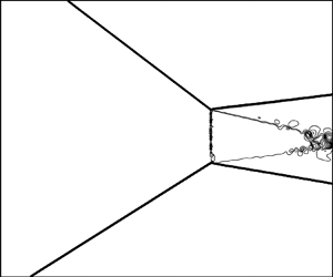
To limit the size of the parameter space, we start with the reduced problem of shock reflection between one moving shock wave and a steady shock wave, as displayed in figure 2. In this reduced problem, the lower shock  $i_{2}$ is steady and the upper shock
  $i_{1}$ is moving with a given normal speed
  $\phi _{n}$ (positive if moving towards the downstream direction and negative if moving towards the upstream direction). We then discuss how to extend the result of the reduced problem to the general problem of shock reflection between two unsteady incident shock waves which move at different speeds.

Figure 2. The reduced problem of shock reflection between a moving shock wave ( $i_{1}$) and a steady shock wave (
 $i_{2}$).
The shock relations for both steady and unsteady shock waves needed in transition analysis are provided in § 2. In § 3 we provide the method to derive the von Neumann condition and the detachment condition for the reduced shock reflection problem, using a reference frame comoving with the intersection point  $T$ of
  $i_{1}$ and
  $i_{2}$. In § 4.1, the transition criteria will be displayed in both the
  $\beta _{01}\text {--}\beta _{02}$ plane and the
  $\theta _{01}\text {--}\theta _{02}$ plane, for different
  $\phi _{n}$ of shock
  $i_{1}$. In § 4.2, numerical simulation by computational fluid dynamics (CFD) is used to check whether the influence of shock motion on transition predicted by theory is also observed in numerical experiments. In § 5, we give a discussion about the inherent mechanism by which shock motion alters the transition condition. This is done by looking at how the effective parameters (Mach number and shock angles) which determine the transition criteria are changed by shock motion. The functional form of the detachment condition is also used to explain some observed phenomena. In § 6, we show how to extend the results of the reduced problem to the general shock reflection problem where both incident shock waves are moving, with a particular discussion of symmetric shock reflection and shock reflection due to translation of a wedge. Section 7 is devoted to conclusions.
2. Shock relations for steady and moving shock waves
We outline the oblique shock wave relations first for steady shock waves and then for moving shock waves (considering  $i_{1}$ as an example). In this paper,
  $\gamma$ is the ratio of specific heats (we simply consider air so that
  $\gamma =1.4$), the density is
  $\rho$, the pressure is
  $p$, the flow velocity is
  $\boldsymbol {V}=(u,v)$, the Mach number is
  $M$, the sound speed is
  $a=\sqrt {\gamma p/{\rho }}$. For any shock wave, the shock angle is
  $\beta$, the flow deflection angle is
  $\theta$. We use subscript
  $0$ to denote inflow stream conditions.
2.1. Oblique shock wave relations for steady shock waves
Shock relations relate the downstream conditions (here denoted with subscript  $d$) to upstream conditions (with subscript
  $u$). For steady oblique shock waves, we generally specify the upstream flow conditions (such as the Mach number
  $M_{u}$, density
  ${{\rho }}_{u}$ and pressure
  $p_{u}$) and the flow deflection angle
  $\theta _{ud}$ or shock angle
  $\beta _{ud}$. The shock angle is related to the flow deflection angle through the shock angle relation
 \begin{equation} \tan \theta_{ud}=f_{\theta}(M_{u},\beta_{ud}),\quad f_{\theta}({M,\beta })=\frac{2\left( {M}^{2}{\sin}^{2}{\beta}-1\right) }{\left( {M}^{2}\left( \gamma+\cos{2\beta}\right) +2\right) \tan{\beta}}. \end{equation}
For given  $M_{u}$ and
  $\theta _{ud}$, the shock angle relation gives two values of
  ${\beta }_{ud}$. The smaller value
  ${\beta }$ corresponds to a weak solution and the larger value corresponds to a strong solution. In certain occasions, it is the shock angle
  $\beta _{ud}$ that is prescribed and (2.1a,b) is then used to obtain
  $\theta _{ud}$.
Once  $\beta _{ud}$ is known, the downstream flow conditions (such as the Mach number
  $M_{d}$, density
  ${{\rho }}_{d}$ and pressure
  $p_{d}$) are obtained from the steady oblique shock wave relations
 \begin{equation} M_{d}^{2}=f_{M}(M_{u},\beta_{ud}),\quad {{\rho}}_{d}={{\rho}}_{u}f_{{{\rho} }}(M_{u},\beta_{ud}),\quad p_{d}=p_{u}f_{p}(M_{u},\beta_{ud}), \end{equation}
where
 \begin{equation} \left. \begin{gathered} f_{M}(M,{\beta)}=\frac{\left( \gamma-1\right) {M}^{2}+2}{2\gamma{M}^{2} {\sin}^{2}{\beta}-\left( \gamma-1\right) }+\frac{2{M}^{2}{\cos}^{2}{\beta} }{\left( \gamma-1\right) {M}^{2}{\sin}^{2}{\beta}+2},\\ f_{{{\rho}}}(M,\beta)=\frac{(\gamma+1){M}^{2}{\sin}^{2}{\beta}}{(2\gamma -1){M}^{2}{\sin}^{2}{\beta}},\\ f_{p}(M,{\beta)}=1+\frac{2\gamma}{\gamma+1}\left( {M}^{2}{\sin}^{2}{\beta }-1\right). \end{gathered} \right\} \end{equation}
With  $V=a\times M$, the velocity components normal (with subscript
  $n$) and tangent (with subscript
  $\tau$) to the shock wave are
 \begin{equation} \left. \begin{gathered} V_{n,u}=V_{u}\sin \beta_{ud},V_{n,d}=V_{d}\sin \left( \beta_{ud}-\theta _{ud}\right), \\ V_{\tau,u}=V_{u}\cos \beta_{ud},V_{\tau,d}=V_{d}\cos(\beta_{ud}-\theta_{ud}). \end{gathered} \right\} \end{equation}
 The shock detaches at the detached angle  $\theta =\theta ^{(max)}(M_{0})$ determined by
  $({\partial f_{\theta }({M_{u},\beta })})/({\partial \beta })=0$. For an upstream Mach number
  $M_{u}$, the expression for the detached angle is
 \begin{equation} \left. \begin{gathered} \sin^{2}\beta_{m}=\frac{1}{\gamma M_{u}^{2}}\left[\frac{\gamma+1}{4}M_{u} ^{2}-1+\sqrt{(1+\gamma)\left(1+\frac{\gamma-1}{2}M_{u}^{2}+\frac{\gamma+1}{16} M_{u}^{4}\right)}\right],\\ \tan \theta^{(max)}=\frac{2[(M_{u}^{2}-1)\tan^{2}\beta_{m}-1]}{\tan \beta _{m}[(\gamma M_{u}^{2}+2)(1+\tan^{2}\beta_{m})+M_{u}(1-\tan^{2}\beta_{m})]}. \end{gathered} \right\} \end{equation}
2.2. Unsteady shock wave relations
For moving shock waves, if the flow conditions are defined in the frame comoving with the shock wave, then the shock wave relations (2.1a,b), (2.2a–c) and (2.3) can still be used to relate the downstream flow conditions (defined on the moving frame) to the upstream conditions (defined on the moving frame). In the following we need shock relations and flow quantities defined on the ground frame. Note that shock relations for moving oblique shock waves are provided by Emanuel & Yi (Reference Emanuel and Yi2000).
Consider just the reduced problem shown in figure 2. Since shock  $i_{2}$ is steady we only consider unsteady shock relations for
  $i_{1}$. These relations relate the flow parameters in region (1) downstream of shock
  $i_{1}$ to those in the upstream region (0). Here we will make the role of the shock speed
  $\phi _{n}$ of shock
  $i_{1}$ appear explicitly.
On the ground frame, the orientation of shock wave  $i_{1}$ is defined by its unit vector normal to the shock wave
  $\boldsymbol {n}$, and the unit vector parallel to the shock wave
  $\boldsymbol {\tau }$. We require the vector
  $\boldsymbol {n}$ to point in the downstream direction and
  $\boldsymbol {\tau }$ in the tangent velocity direction.
Apart from the upstream flow condition (with subscript  $0$), we also prescribe the shock angle
  $\beta _{01}$ or the flow deflection angle
  $\theta _{01}$. In the end of this subsection, we will show how to compute
  $\beta _{01}$ if
  $\theta _{01}$ and
  $\phi _{n}$ are prescribed, and to compute
  $\theta _{01}$ if
  $\beta _{01}$ and
  $\phi _{n}$ are prescribed. For the moment, we just prescribe
  $\beta _{01}$.
Giving  $\boldsymbol {V}_{0}$ and the shock angle
  $\beta _{01}$, the normal and tangent velocity components in region (0) are given by
 \begin{equation} \left. \begin{gathered} V_{n,0}=\boldsymbol{V}_{0}\boldsymbol{\cdot} \boldsymbol{n}=V_{0}\sin \beta_{01},\\ V_{\tau,0}=\boldsymbol{V}_{0}\boldsymbol{\cdot} \boldsymbol{\tau}=V_{0}\cos \beta_{01}. \end{gathered} \right\} \end{equation}
 We will consider the case with  $p_{1}>p_{0}$, so that the unsteady shock
  $i_{1}$ belongs to the first family, in that its normal speed
  $\phi _{n}$ is related to the pressure jump by the following classical relation in shock dynamics (Ben-Dor, Igra & Elperin Reference Ben-Dor, Igra and Elperin2001):
 \begin{equation} \phi_{n}=V_{n,0}-a_{0}\sqrt{\frac{\gamma+1}{2\gamma}\frac{p_{1}}{p_{0}} +\frac{\gamma-1}{2\gamma}}. \end{equation}
Since  $p>p_{0}$, we have
 \begin{equation} -\infty<\phi_{n}< V_{0,n}-a_{0}=\left( M_{0,n}-1\right) a \end{equation}
so that the maximal value of  $\phi _{n}$ is limited.
The shock speed  $\phi _{n}$ is considered as a given parameter in this paper, the pressure
  $p_{1}$ is obtained from (2.7), as
 \begin{equation} p_{1}=\frac{1}{\gamma+1}\left( 1-\gamma+\frac{2\gamma}{a_{0}^{2}}\left( \phi_{n}-V_{n,0}\right) ^{2}\right) p_{0}. \end{equation}
 The downstream flow speed in the direction normal to the shock wave  $V_{n,1}=\boldsymbol {V}_{1}\boldsymbol {\cdot } \boldsymbol {n}$ is then given by (see also Ben-Dor et al. Reference Ben-Dor, Igra and Elperin2001)
 \begin{equation} V_{n,1}=V_{n,0}-\frac{a_{0}}{\gamma}\left(\frac{p_{1}}{p_{0}}-1\right)\left(\frac{\gamma +1}{2\gamma}\frac{p_{1}}{p_{0}}+\frac{\gamma-1}{2\gamma}\right)^{-{1}/{2}} \end{equation}
and the density  $\rho _{1}$ is given by the well known density–pressure relation
 \begin{equation} \frac{\rho_{1}}{\rho_{0}}=\frac{\dfrac{\gamma+1}{\gamma-1}\dfrac{p_{1}}{p_{0} }+1}{\dfrac{\gamma+1}{\gamma-1}+\dfrac{p_{1}}{p_{0}}}. \end{equation}
 The tangent component of the velocity does not change across the shock wave, independent of the shock speed. Thus  $V_{\tau,1}=V_{\tau,0}$, or
 \begin{equation} V_{\tau,1}=V_{\tau,0}=V_{0}\cos \beta_{01} \end{equation}
if (2.6) is used for  $V_{\tau,0}$.
Now we derive the shock angle relation of unsteady shock wave similar to (2.1a,b) for a steady one. By  $V_{\tau,1}=V_{1}\cos ( \beta _{01}-\theta _{01})$ and
  $V_{n,1}=V_{1}\sin ( \beta _{01} -\theta _{01})$, we have
 \begin{equation} \tan \left( \beta_{01}-\theta_{01}\right) =\frac{V_{n,1}}{V_{\tau,1}}. \end{equation}
Putting (2.10) and (2.12) into (2.13) gives the following shock angle relation for unsteady shock wave:
 \begin{equation} \tan \left( \beta_{01}-\theta_{01}\right) =\dfrac{\sin \beta_{01}-\dfrac {1}{\gamma M_{0}}(\sigma-1)\left(\dfrac{\gamma+1}{2\gamma}\sigma+\dfrac{\gamma -1}{2\gamma}\right)^{-{1}/{2}}}{\cos \beta_{01}}, \end{equation}
where
 \begin{equation} \sigma=\frac{1}{\gamma+1}\left( 1-\gamma+2\gamma M_{0}^{2}\left( \frac{M_{\phi_{n}}}{M_{0}}-\sin \beta_{01}\right) ^{2}\right). \end{equation}
In (2.15),  $M_{\phi _{n}}$ is the shock speed Mach number defined by
 \begin{equation} M_{\phi_{n}}=\frac{\phi_{n}}{a_{0}}. \end{equation}
 The appearance of  $M_{\phi _{n}}$ in the shock angle relation suggests that the influence of shock speed should be accounted for in terms of
  $M_{\phi }$ defined by (2.16). This may explain why Naidoo & Skews (Reference Naidoo and Skews2011, Reference Naidoo and Skews2014) used a similar shock speed Mach number in studying the effect of wedge rotation on transition. Note that Naidoo & Skews (Reference Naidoo and Skews2011, Reference Naidoo and Skews2014) defined this Mach number based on the linear shock speed due to rotation.
Figure 3 displays the curves  $\theta _{01}=\theta _{01} (M_{0},M_{\phi _{n}},\beta _{01})$ given by (2.14) at
  $M_{0}=4.96$, for
  $M_{\phi _{n}}=-0.1$,
  $0$ and
  $0.1$. It is seen that when
  $M_{\phi _{n}}<0$ or
  $M_{\phi _{n}}>0$, the flow deflection angle is increased or decreased, compared with
  $M_{\phi _{n}}=0$.

Figure 3. Shock angle curves for three different shock speeds for  $M_{0}=4.96$.
3. Method to obtain transition criteria for the reduced problem
The transition criteria are studied here on an equivalent problem defined by choosing a reference frame comoving with the intersection point  $T$ of shock
  $i_{1}$ and
  $i_{2}$ (see figure 2) and expressed in terms of flow parameters defined on the ground frame. On this equivalent problem, the method for transition criteria of steady shock reflection can be directly applied to study the influence of shock speed. However, the analysis is not as simple as it appears, since the inflow Mach number will be changed by this choice of frame. Below we first define the comoving reference frame. We then provide the method to study the transition criteria. We only consider the von Neumann condition and detachment condition. The results will be displayed in § 4.
3.1. Equivalent flow conditions defined in the reference frame comoving with the intersection point  $T$
$T$

The flow parameters in the ground frame for the reduced problem are displayed in figure 4(a). Now we choose a reference frame comoving with the intersection point  $T$ of shock
  $i_{1}$ and
  $i_{2}$. In this reference frame, which moves at velocity
  $\boldsymbol {\phi }_{T}$ to be determined below, the flow parameters, called equivalent flow parameters, will be denoted using an overbar (e.g.
  $\bar {M}$ is the Mach number seen in the moving reference frame), as shown in figure 4(b).

Figure 4. Illustration of flow parameters for the reduced problem: (a) ground frame; (b) frame comoving with  $T$.
$T$.
First we derive the velocity  $\boldsymbol {\phi }_{T}=(\phi _{Tx},\phi _{Ty})$ of the intersection point
  $T$ of shock
  $i_{1}$ and
  $i_{2}$. This velocity is due to the motion of shock
  $i_{1}$. Since
  $T$ also moves along the tangent direction of shock
  $i_{2}$, the velocity vector of
  $T$ and the velocity of shock
  $i_{1}$ (normal to
  $i_{1}$) form the two sides of a rectangular triangle such that
  $-{{\phi }_{n}=}\phi _{T}\sin ({{\beta }_{01}+{\beta }_{02})}$. See figure 5 for a schematic view of the interaction location with all relevant angles and the upper incident shock and interaction point velocity vectors. Since
  $\phi _{Tx}=-\phi _{T}\cos {{\beta }_{02}}$ and
  $\phi _{Ty} =-\phi _{T}\sin {{\beta }_{02}}$, we obtain
 \begin{equation} \phi_{Tx}={{\phi}_{n}}\frac{\cos{{\beta}_{02}}}{\sin({{\beta}_{01}+{\beta }_{02})}},\quad \phi_{Ty}={{\phi}_{n}}\frac{\sin{{\beta}_{02}}}{\sin ({{\beta}_{01}+{\beta}_{02})}}. \end{equation}
Figure 5. Schematic view of parameters in relation (3.1a,b).
For the steady shock  $i_{2}$, if its shock angle
  $\beta _{02}$ is given, then (2.1a,b) is used for
  $\theta _{02}$. If
  $\theta _{02}$ is prescribed, then
  $\beta _{02}$ is obtained from (2.1a,b). The flow parameters in region (2) are determined by (2.2a–c). With the normal and tangent velocities
  $V_{n}$ and
  $V_{\tau }$ in region (2) determined from (2.4), we get
 \begin{equation} \left. \begin{gathered} u_{2}=V_{n,2}\sin \beta_{02}+V_{\tau,2}\cos \beta_{02},\\ v_{2}={-}V_{n,2}\cos \beta_{02}+V_{\tau,2}\sin \beta_{02}. \end{gathered} \right\} \end{equation}
 For shock  $i_{1}$, which has a normal speed
  ${{\phi }_{n}}$, if
  $\beta _{01}$ is prescribed, then (2.14) is solved for
  $\theta _{01}$. If
  $\theta _{01}$ is prescribed, then (2.14) is solved for
  $\beta _{01}$. With the normal and tangent velocities determined by (2.10) and (2.12), the flow velocity components in region (1) are then computed by
 \begin{equation} \left. \begin{gathered} u_{1}=V_{n,1}\sin \beta_{01}+V_{\tau,1}\cos \beta_{01},\\ v_{1}=V_{n,1}\cos \beta_{01}-V_{\tau,1}\sin \beta_{01}. \end{gathered} \right\} \end{equation}
 With the velocity  $\boldsymbol {\phi }_{T}=(\phi _{Tx},\phi _{Ty})$ determined by (3.1a,b), the equivalent velocity components and Mach number in region
  $(k)$ with
  $k=0,1,2,3,4$ are computed by
 \begin{equation} \left. \begin{gathered} \bar{u}_{k}=u_{k}-\phi_{Tx},\\ \bar{v}_{k}=v_{k}-\phi_{Ty},\\ \bar{M}_{k}=\frac{\sqrt{\bar{u}_{k}^{2}+\bar{v}_{k}^{2}} }{\bar{a}_{k}}. \end{gathered} \right\} \end{equation}
Note that the pressure, density and sound speed do not change with the frame, so we have
 \begin{equation} \bar{p}_{k}=p_{k},\quad \bar{\rho}_{k}=\rho_{k}, \quad \bar{a}_{k}=a_{k}. \end{equation}
In the ground frame, the flow deflection angle in region  $(0)$ is
  ${{\theta }_{0}=0}$ and the equivalent flow deflection angle in region
  $(0)$ (with respect to the horizontal direction) is given by
 \begin{equation} \bar{\theta}_{0}=\arctan \frac{\bar{v}_{0}}{\bar{u}_{0}}. \end{equation}
If  $\phi _{n}<0$, so that
  $T$ moves along the upstream direction, then,
  $\bar {u}_{0}>0$,
  $\bar {v}_{0}>0$ and
  $\bar {\theta }_{0}>0$.
The equivalent shock angles (see figure 4b for notation) are given by
 \begin{equation} \left. \begin{gathered} \bar{\beta}_{01}=\beta_{01}+\bar{\theta}_{0},\\ \bar{\beta}_{02}=\beta_{02}-\bar{\theta}_{0} \end{gathered} \right\} \end{equation}
and the equivalent flow deflection angles satisfy
 \begin{equation} \left. \begin{gathered} \bar{\theta}_{01}=\bar{\theta}_{0}-\arctan \frac{\bar{v}_{1}}{\bar{u}_{1}},\\ \bar{\theta}_{02}=\arctan \frac{\bar{v}_{2}}{\bar{u}_{2} }-\bar{\theta}_{0}. \end{gathered} \right\} \end{equation}
Finally, the shock relations
 \begin{equation} {{\bar{p}}_{1}}={{\bar{p}}_{0}}{{f}_{p}}(\bar{M}{_{0}},{{\bar{\beta} }_{01}}),\quad {{\bar{p}}_{2}}={{\bar{p}}_{0}}{{f}_{p}}(\bar{M}{_{0} },{{\bar{\beta}}_{02}}) \end{equation}
are used to find the equivalent pressures  ${{\bar {p}}_{1}}$ and
  ${{\bar {p} }_{2}}$ downstream of shock
  $i_{1}$ and shock
  $i_{2}$. In fact these pressures are invariant under frame transformation.
Note that the shock system (including shock angles and flow deflection angles) displayed in figure 4(a) is obtained using the real conditions  $M_{0}=4.96$,
  ${{\theta }_{01}=25}^{\circ }$,
  ${{\theta }_{02}=15}^{\circ }$,
  $\phi _{n}=-2a_{0}$. From these conditions we get
  $\beta _{01}=10.863^{\circ }$ by (2.14) and
  $\beta _{02}=24.405^{\circ }$ by (2.1a,b). Using (3.1a,b) we get
  $\phi _{Tx}=-3.154a_{0}$ and
  $\phi _{Ty}=-1.431a_{0}$. Note that due to shock motion with
  $\phi _{n}=-2a_{0}$, the shock angle
  $\beta _{01}$, which should be
  $35.858^{\circ }$ in the case of steady shock, is reduced to
  $10.863^{\circ }$. Using (3.6), (3.4), (3.7) and (3.8) we obtain
  $\bar {\theta }_{0}=10.003^{\circ }$,
  $\bar {M}_{0}=8.240$,
  $\bar {\theta } _{01}=15.132^{\circ }$,
  $\bar {\theta }_{02}=9.0465^{\circ }$,
  $\bar {\beta }_{01}=20.866^{\circ }$ and
  $\bar {\beta }_{02}=14.402^{\circ }$. These shock angles are used to obtain the illustration in figure 4(b).
3.2. Method to determine the von Neumann condition and detachment condition
For steady asymmetrical shock reflection, the theory for critical conditions of transition from RR to MR has been given by Li et al. (Reference Li, Chpoun and Ben-Dor1999) and Ivanov et al. (Reference Ivanov, Ben-Dor, Elperin, Kudryavtsev and Khotyanovsky2002). Now we provide the method to derive the transition criteria for the reduced problem with  $i_{1}$ moving at
  $\phi _{n}$. The transition criteria now depend on the shock speed
  $\phi _{n}$ (shock
  $i_{1}$) so that the von Neumann condition has the functional form
  ${\theta _{02}=\theta _{02}^{(N)}}(M_{0},\theta _{01},\phi _{n})$ and the detachment condition has the functional form
  ${\theta _{02}=\theta _{02}^{(D)} }(M_{0},\theta _{01},\phi _{n})$. Similar functional forms can be defined for shock angles
  $\beta _{01}$ and
  $\beta _{02}$.
It seems to be very simple and straightforward to obtain the transition criteria to account for  $\phi _{n}$, by simply putting the equivalent flow conditions into the analysis of transition criteria for steady asymmetric shock reflection. However, while searching for
  ${\theta _{02}}$ (or
  $\beta _{02}$) such that the von Neumann condition or the detachment condition holds, the inflow Mach number
  $\bar {M}{_{0}}$ cannot be made fixed, due to the fact that the velocity of
  $T$ and thus
  $\bar {M}{_{0}}$ also depend on
  ${\theta _{02}}$.
Now, for a given inflow Mach number  $M{_{0}}$, flow deflection angle
  ${{\theta }_{01}}$ and shock speed
  $\phi _{n}$ of shock
  $i_{1}$, we look for
  ${\theta _{02}}$ to meet the von Neumann condition and detachment condition in the frame comoving with
  $T$. We provide below the steps to be followed in the algorithm to find these transition criteria.
(i) Step 1. The flow velocity components
$u_{1}$ and $v_{1}$ in region (1) are computed using (3.3). A series of ${\theta _{02}}$ is considered for searching the von Neumann condition and detachment condition, using the method provided below.(ii) Step 2. For any
${\theta _{02}}$ thus preprescribed, the velocity of $T$ is computed by (3.1a,b), the flow velocity components in (2) are computed using (3.2). The equivalent flow parameters $\bar {M}_{0}$, $\bar {M}_{1}$, $\bar {M}_{2}$, $\bar {\beta }_{01}$, $\bar {\beta }_{02}$, $\bar {\theta }_{01}$ and $\bar {\theta }_{02}$ are computed by (3.4)–(3.8), and $\bar {p}_{1},\bar {p}_{2}$ by (3.9a,b).(iii) Step 3. The detachment condition is searched. Referring to figure 6 for notations for shock angles and flow deflection angles, the pressures
${{\bar {p}}_{3}}$ and ${{\bar {p}}_{4}}$ downstream of the reflected shock waves $r_{1}$ and $r_{2}$ are computed by


 \begin{equation} \left. \begin{gathered} \tan \bar{\theta}_{13}={{f}_{\beta}}(\bar{M}_{1}, {{\bar{\beta} }_{13}}),\quad {{\bar{p}}_{3}}={{\bar{p}}_{1}}{{f}_{p}}(\bar{M}{_{1}} ,{{\bar{\beta}}_{13}}),\\ \tan \bar{\theta}_{24}={{f}_{\beta}}(\bar{M}{_{2}},{{\bar{\beta} }_{24}}),\quad {{\bar{p}}_{4}}={{\bar{p}}_{2}}{{f}_{p}}(\bar{M}{_{2}} ,{{\bar{\beta}}_{24}}). \end{gathered} \right\} \end{equation}
Figure 6. The equivalent flow deflection angles in the comoving frame.
Let the slipline  $s$ (see figure 6) deflect at an angle
  ${{\bar {\theta }}}_{s}$ (assumed positive if the it deflects in the clockwise direction). The expressions in (3.10) are solved along with the following flow parallel condition
 \begin{equation} \left. \begin{gathered} {\bar{\theta}}_{13}={\bar{\theta}}_{01}-{\bar{\theta}}_{0}-{\bar{\theta}}_{s},\\ {\bar{\theta}}_{24}={\bar{\theta}}_{02}+{\bar{\theta}}_{0}+{\bar{\theta}}_{s} \end{gathered} \right\} \end{equation}
and pressure balance condition
 \begin{equation} {{\bar{p}}_{3}={\bar{p}}_{4}}. \end{equation}
 The satisfaction of (3.11) and (3.12) means that the polar of the two reflected shock waves have intersected. The detachment condition  $\theta _{02}=$
  $\theta _{02}^{(D)}(M_{0},\theta _{01},\phi _{n})$ is the condition for
  ${{\bar {\theta }}_{02}}$ such that the polar of the reflected shock originated from (
 ${{\bar {\theta }}_{02}},{{\bar {p}}_{2}}$), calculated from (3.10)), is tangent to the polar of the reflected shock originated from (
 ${{\bar {\theta }}_{01}},{{\bar {p}}_{1}}$), calculated from (3.10).
(iv) Step 4. The von Neumann condition is searched. Let
${{\bar {p} }_{m}}$ be the pressure downstream of a strong shock wave with flow deflection angle $\bar {\theta }_{0}+{{\bar {\theta }}}_{s}$ and with the upstream Mach number $\bar {M}{_{0}}$. Let $\beta _{s}$ be the strong shock wave solution of $\tan (\bar {\theta }_{0}+{{\bar {\theta }}}_{s})={{f}_{\beta } }(\bar {M}_{0},{{\bar {\beta }}_{s}})$, then
(3.13)We still use (3.10), (3.11) and (3.12) to find the pressure\begin{equation} {{\bar{p}}_{m}}={{\bar{p}}_{0}}\left( 1+\frac{2\gamma}{\gamma+1}\left( {{\left( \bar{M}{_{0}}\sin \bar{\beta}_{s}\right) }^{2}}-1\right) \right). \end{equation}${{\bar {p}}_{3}}$ and ${{\bar {p}}_{4}}$ behind the reflected shock waves $r_{1}$ and $r_{2}$. The von Neumann condition $\theta _{02}=$ $\theta _{02}^{(N)}(M_{0},\theta _{01},\phi _{n})$ is reached when


 \begin{equation} \bar{p}_{m}=\bar{p}_{3} =\bar{p}_{4}. \end{equation}
Algorithm gives the pseudocode to obtain the transition conditions.

4. Transition criteria and numerical validation
In this section, we display the transition criteria accounting for the influence of the shock speed for the reduced problem, predicted by theory. We then provide numerical validation.
4.1. The transition criteria for the reduced problem predicted by theory
We have computed the transition criteria for both  $M_{0}=4.96$ and
  $M_{0}=3.96$, with seven shock speeds
  $\phi _{n}=0$,
  $\phi _{n}=\pm a_{0}/10$,
  $\phi _{n}=\pm 2(a_{0})/10$,
  $\phi _{n}=\pm 4(a_{0})/10$. The difference of the transition criteria for
  $\phi _{n}\neq 0$ compared with that for
  $\phi _{n}=0$ reflects the influence of the shock speed
  $\phi _{n}$ on transition. The transition criteria for
  $\phi _{n}=0$ recover the steady state criteria of Li et al. (Reference Li, Chpoun and Ben-Dor1999) and Ivanov et al. (Reference Ivanov, Ben-Dor, Elperin, Kudryavtsev and Khotyanovsky2002). The conclusion is similar for both Mach numbers so we only display results for
  $M_{0}=4.96$.
If the von Neumann condition is lowered or elevated due to shock motion, the transition from MR to RR is delayed or advanced. If the detachment condition is lowered or elevated due to shock motion, the transition from RR to MR is advanced or delayed.
The transition criteria in the  $\beta _{01}\text {--}\beta _{02}$ plane are displayed in figure 7(a) for
  $\phi _{n}<0$ and in figure 7(b) for
  $\phi _{n}>0$.

Figure 7. Transition criteria in the  $\beta _{01}\text {--}\beta _{02}$ plane with
  $M_{0}=4.96$. The arrow
  $\nearrow$ indicates the direction of increasing
  $\vert M_{\phi _{n}} \vert$. (a) For
  $M_{\phi _{n}}=0$ (steady),
  $M_{\phi _{n}}=-0.1$,
  $M_{\phi _{n}}=-0.2$ and
  $M_{\phi _{n}}=-0.4$. (b) For
  $M_{\phi _{n}}=0$ (steady),
  $M_{\phi _{n}}=0.1$,
  $M_{\phi _{n}}=0.2$ and
  $M_{\phi _{n}}=0.4$.
First consider the von Neumann condition. For shock  $i_{1}$ moving with
  $\phi _{n}<0$ and
  $\phi _{n}>0$, the von Neumann condition is globally lowered and elevated, respectively, compared with
  $\phi _{n}=0$. Thus, the motion of shock
  $i_{1}$ towards the upstream direction (
 $\phi _{n}<0$) delays transition from MR to RR. On the contrary, for shock
  $i_{1}$ moving along the downstream direction, i.e. for
  $\phi _{n}>0$, the von Neumann condition is elevated compared with
  $\phi _{n}=0$. Thus, the motion of shock
  $i_{1}$ with
  $\phi _{n}>0$ advances transition from MR to RR. The influence of shock motion on transition becomes less important for large
  $\beta _{01}$.
Now consider the detachment condition. We observe that the influence of shock motion on the detachment condition is not monotonic. In figure 7, we marked two dividing points  ${\rm a}$ and
  ${\rm b}$ showing non-monotonicity, across which the influence of shock motion changes sign. In figure 7(a) which is for
  $\phi _{n}<0$, we have
  $\beta _{01}=\beta _{a}\approx 19^{\circ }$ at
  ${\rm a}$ and
  $\beta _{01}=\beta _{b}\approx 37.8^{\circ }$ at
  ${\rm b}$. The detachment condition for
  $\phi _{n}<0$ is lowered compared with
  $\phi _{n}=0$ when
  $\beta _{01}<\beta _{a}$, and elevated when
  $\beta _{a}<\beta _{01}<\beta _{b}$, and lowered again when
  $\beta _{01}>\beta _{b}$. For
  $\phi _{n}>0$, similar behaviour is observed: the detachment condition is elevated compared with
  $\phi _{n}=0$ when
  $\beta _{01}<23.3^{\circ }$, lowered when
  $23.3^{\circ }< \beta _{01}<41.5^{\circ }$, and elevated again when
  $\beta _{01}>41.5^{\circ }$. The reason to have these points (
 ${\rm a}$ and
  ${\rm b}$) will be discussed in § 5.
In summary, for the detachment condition, the influence of shock motion is not monotonic, i.e. it is not globally elevated or lowered by shock motion. Moreover, the influence of shock motion on the detachment condition is small for both small and large  $\beta _{01}$, and smaller than that on the von Neumann condition for small
  $\beta _{01}$. These observed behaviours will be further displayed at the end of this subsection using derivatives of the transition criteria with respect to shock speed.
Now we display the transition criteria in the  $\theta _{01}\text {--}\theta _{02}$ plane. There are two methods to view the influence of shock speed on transition in this plane.
In the first method, the abscissa of  $\theta _{01}$, denoted as
  $\theta _{01}^{(s)}$, is the one associated with the steady case, i.e. for a given
  $\beta _{01}$,
  $\theta _{01}^{(s)}$ is determined by (2.14) with
  $\phi _{n}=0$. Displaying transition criteria in this plane allows the comparison of transition criteria when the shock angle
  $\beta _{01}$ is the same for different shock speeds
  $\phi _{n}$.
The transition criteria in the  $\theta _{01}^{(s)}\text {--}\theta _{02}$ plane are displayed in figure 8(a) for
  $\phi _{n}<0$ and figure 8(b)
  $\phi _{n}>0$. The influence of transition criteria in this plane is similar to that in the
  $\beta _{01}\text {--}\beta _{02}$ plane.

Figure 8. Transition criteria in the  $\theta _{01}^{(s)}-\theta _{02}$ plane with
  $M_{0}=4.96$. (a) For
  $M_{\phi _{n}}=0$ (steady),
  $M_{\phi _{n}} =-0.1$,
  $M_{\phi _{n}}=-0.2$ and
  $M_{\phi _{n}}=-0.4$. (b) For
  $M_{\phi _{n}}=0$ (steady),
  $M_{\phi _{n}}=0.1$,
  $M_{\phi _{n}}=0.2$ and
  $M_{\phi _{n} }=0.4$.
In the second method, the abscissa of  $\theta _{01}$, denoted as
  $\theta _{01}^{(r)}$, is the real local one, that is associated with the shock speed
  $\phi _{n}$, i.e. for a given
  $\beta _{01}$,
  $\theta _{01}^{(r)}$ is determined by the unsteady shock angle relation (2.14).
The transition criteria in the  $\theta _{01}^{(r)}\text {--}\theta _{02}$ plane are displayed in figure 9(a) for
  $\phi _{n}<0$ and figure 9(b) for
  $\phi _{n}>0$. It is interesting to note that, for the von Neumann condition, the influence of
  $\phi _{n}$ is reversed in this plane compared with the transition criteria displayed in the
  $\theta _{01}^{(s)}\text {--}\theta _{02}$ plane. For shock
  $i_{1}$ moving along the upstream direction, i.e. for
  $\phi _{n}<0$, both the von Neumann condition and the detachment condition are elevated compared with
  $\phi _{n}=0$. This influence becomes larger when
  $\theta _{01}$ is larger. On the contrary, for shock
  $i_{1}$ moving along the downstream direction, i.e. for
  $\phi _{n}>0$, both of the von Neumann condition and the detachment condition are lowered compared with
  $\phi _{n}=0$. This influence becomes larger when
  $\theta _{01}$ is larger.

Figure 9. Transition criteria in the  $\theta _{01}^{(r)}\text {--}\theta _{02}$ plane with
  $M_{0}=4.96$. (a) For
  $M_{\phi _{n}}=0$ (steady),
  $M_{\phi _{n}} =-0.1$,
  $M_{\phi _{n}}=-0.2$ and
  $M_{\phi _{n}}=-0.4$. (b) For
  $M_{\phi _{n}}=0$ (steady),
  $M_{\phi _{n}}=0.1$,
  $M_{\phi _{n}}=0.2$ and
  $M_{\phi _{n} }=0.4$.
The influence of shock motion on the transition criteria can also be seen from the derivatives of these criteria with respective to the shock speed. For  $\beta _{02}^{(N)}$ and
  $\beta _{02}^{(D)}$ these derivatives may be defined by
 \begin{equation} \beta_{\phi_{n}}^{(N)}=\frac{\textrm{d}\beta_{02}^{(N)}}{\textrm{d}M_{\phi_{n}}},\quad \beta_{\phi _{n}}^{(D)}=\frac{\textrm{d}\beta_{02}^{(D)}}{\textrm{d}M_{\phi_{n}}} \end{equation}
and for  $\theta _{02}^{(N)}$ and
  $\theta _{02}^{(D)}$ they may be defined by
 \begin{equation} \theta_{\phi_{n}}^{(N)}=\frac{\textrm{d}\theta_{02}^{(N)}}{\textrm{d}M_{\phi_{n}}},\quad \theta _{\phi_{n}}^{(D)}=\frac{\textrm{d}\theta_{02}^{(D)}}{\textrm{d}M_{\phi_{n}}}. \end{equation}
 The exact values of these derivatives could be obtained from linear expansion of the expressions for transition criteria, presented in § 3.2. However, such an approach leads to a large number of algebraic formulae. To reduce the complexity, here we choose to use the approximate values for these derivatives, obtained by the difference between the transition criteria with small  $\phi _{n}$ (here with
  $M_{\phi _{n}}=\pm 0.1$) and the steady state transition criteria, divided by
  $M_{\phi _{n}}$.
The derivatives  $\beta _{\phi _{n}}^{(N)}$ and
  $\beta _{\phi _{n}}^{(D)}$ thus evaluated are displayed in figure 10(a) and the derivatives
  $\theta _{\phi _{n}}^{(N)}$ and
  $\theta _{\phi _{n}}^{(D)}$ for
  $\theta _{01} ^{(r)}$ are displayed in figure 10(b). The behaviour of derivatives
  $\theta _{\phi _{n}}^{(N)}$ and
  $\theta _{\phi _{n}}^{(D)}$ for
  $\theta _{01}^{(s)}$, not displayed here, is similar to that displayed in figure 10(a).

Figure 10. Derivatives of transition criteria for  $M_{0}=4.96$. (a) Derivatives for
  $\beta _{\phi _{n} }^{(N)}$ and
  $\beta _{\phi _{n}}^{(D)}$. (b) Derivatives for
  $\theta _{\phi _{n} }^{(N)}$ and
  $\theta _{\phi _{n}}^{(D)}$.
The influence of shock motion on transition is more clearly seen here from these derivatives than from the transition criteria displayed in figures 7(a) and 7(b). According to figure 10(a), the derivative  $\beta _{\phi _{n}}^{(N)}$ is positive for all
  $\beta _{01}$, showing that with
  $\phi _{n}<0$ the von Neumann condition is lowered globally and with
  $\phi _{n}>0$ it is elevated globally. Moreover, the derivative
  $\beta _{\phi _{n}}^{(N)}$ decreases in magnitude for increasing
  $\beta _{01}$. The derivative
  $\beta _{\phi _{n}}^{(D)}$ is positive for
  $\beta _{01}$ less than some value (point
  ${\rm a}$ of figure 7a), negative when
  $\beta _{01}$ lies between this value and another value (point
  ${\rm b}$ of figure 7a), and positive again when
  $\beta _{01}$ is larger, showing more clearly the non-monotonicity observed in figures 7(a) and 7(b). The derivatives
  $\beta _{\phi _{n}}^{(D)}$ are smaller in magnitude than the derivatives
  $\beta _{\phi _{n}}^{(N)}$ even for small
  $\beta _{01}$.
As displayed in figure 10(b), the derivatives  $\theta _{\phi _{n}}^{(N)}$ and
  $\theta _{\phi _{n}}^{(D)}$ are negative for all
  $\theta _{01}^{(r)}$, showing that, with
  $\phi _{n}<0$, the von Neumann condition and the detachment condition are elevated globally and, with
  $\phi _{n}>0$, the von Neumann condition and the detachment condition are lowered globally.
The reason for these observations will be discussed in § 5.
4.2. Numerical validation
Now we use numerical simulation to check, for some particular cases, if the influence of shock motion on transition, predicted by theory, is correct. In numerical simulations, the unsteady Euler equations in gas dynamics are solved using the second-order upwind advection upstream splitting method (known as AUSM) scheme, with a grid of  $400\times 400$ points. We have checked that further refining the grid does not alter the results with regard to the transition condition.
In the usual shock reflection problems, the transition from RR to MR or MR to RR can be studied, both numerically and experimentally, by entering or leaving the DS domain through wedge angle variation (cf. Chpoun et al. Reference Chpoun, Passerel, Li and Ben-Dor1995; Vuillon et al. Reference Vuillon, Zeitoun and Ben-Dor1995) or through inflow Mach number variation (Ivanov et al. Reference Ivanov, Ben-Dor, Elperin, Kudryavtsev and Khotyanovsky2001). However, this procedure cannot be used in the present problem since we want the shock speed to be fixed at constant. The influence of shock motion on transition cannot be checked in numerical simulations using wedge rotation like that used by Naidoo & Skews (Reference Naidoo and Skews2011, Reference Naidoo and Skews2014), since wedge rotation involves non-constant shock speed and the present study is merely for constant speed. This difficulty is overcome here by using the technique of forced transition in the DS domain. Specifically, we use the forced transition method of Li et al. (Reference Li, Gao and Wu2011). In this method, we first compute an RR numerical result. We then superimpose a local discontinuity near the reflection point on numerical solutions with RR. This local discontinuity is defined in a similar way as for the initial condition of a one-dimensional Riemann problem. Specifically, it uses the conditions downstream of a moving shock wave as the perturbation state and this state is defined in an area centred at the intersection point of the two incident shock waves, which spans  $7\times 5$ grid points. See Li et al. (Reference Li, Gao and Wu2011) for more details for how to define such a local discontinuity.
Two sets of conditions are considered: the first set is with  $M_{\phi _{n}} \leq 0$; the second set is with
  $M_{\phi _{n}}>0$.
Nines cases are considered for  $M_{\phi _{n}}\leq 0$ and the corresponding input conditions (
 $M_{0}$,
  $\theta _{01}$ and
  $\beta _{01},\theta _{02}$ and
  $\beta _{02},M_{\phi _{n}}$) are given in table 1.
Table 1. Comparison of reflection types predicted by theory and CFD. Here FT means forced transition with a local discontinuity perturbation.

The eighth column is the possible reflection configuration (RR, DS, MR) predicted by theory (§§ 3 and 4), the ninth column is the reflection observed from numerical simulation without applying forced transition, and the last column is the reflection observed from numerical simulation without applying forced transition. If we get RR without applying forced transition and then MR after forced transition is applied, then we are in the DS domain. We see that apart from case 4, which is close to the von Neumann condition, theory agrees well with numerical simulations.
The reflection types predicted by CFD are also shown in figure 11. The filled circles represents that the CFD result first shows RR and after the forced transition method shows MR, the round doughnut represents that the CFD result first shows MR without the forced transition method being used.

Figure 11. The CFD results near the detachment condition for  $M_{0}=4.96,$
  $M_{\phi _{n}}=-0.1$ compared with the theoretical curve.
To see some details we only show the flow for case 1 and case 2. The two incident shock waves are steady for case 2, while the upper incident shock wave has  $M_{\phi _{n}}=-0.1$ for case 1. According to the transition criteria displayed in figure 9(a), case 1 is in the DS domain and near the detachment condition, case 2 is in the MR domain. This difference of solution domain is purely caused by shock motion according to the theory, so if DS and MR can be observed numerically for case 1 and case 2, respectively, this theory is said to be confirmed for a particular choice of test condition.
Figure 12 displays, for case 1, the Mach contours at various instants before and after forced transition. Figure 12(a) shows Mach contours with RR, obtained before imposing local perturbation. Figure 12(b) displays the Mach contours just at the moment where the local discontinuity for forced transition is superimposed. Figure 12(c–f) display the Mach contours at several instants, after transition to MR by forced transition. This confirms the theoretical prediction that case 1 is in the DS domain.

Figure 12. Mach contours at different instants for case 1: (a) RR before forced transition, (b) RR superimposed with local perturbation and (c–f) evolution of MR after forced transitions.
The Mach contours at a typical instant for case 2 are displayed in figure 13. Theoretically it is in MR region and computation indeed yields MR without the need of forced transition.

Figure 13. Mach contours for case 2.
We consider 10 cases for  $M_{\phi _{n}}>0$, and the corresponding input conditions (
 $M_{0}$,
  $\theta _{01}$ and
  $\beta _{01},\theta _{02}$ and
  $\beta _{02},M_{\phi _{n}}$) are given in table 2. The reflection type predicted by CFD is also displayed in figure 14. As for figure 11, the filled circles represents that the CFD result first shows RR and after the forced transition method shows MR, the round doughnut represents that the CFD result first shows MR without forced transition method used. It is seen that theory agrees with numerical simulations.

Figure 14. The CFD results near the detachment condition for  $M_{0}=4.96,$
  $M_{\phi _{n}}=0.1$ compared with the theoretical curve.
Table 2. Comparison of reflection types for  $M_{0}=4.96,$
  $M_{\phi _{n}} =0.1$. Here FT means forced transition with a local discontinuity perturbation.

5. A discussion on the influence of shock motion
The inherent mechanism by which the transition criteria are altered by shock motion is discussed here through looking at how the effective parameters (Mach number and shock angles), which determine the unsteady transition criteria following the steady ones, are changed by shock motion. Some observed phenomena are also explained by looking at the functional form of the transition criteria.
5.1. The transition criteria for steady shock reflection
In order to understand the influence of shock motion on the transition condition, we need to know the influence of the incident shock angle and the inflow Mach number on transition criteria in steady asymmetric shock reflection. The reason is that the shock motion changes the transition criteria through changing the equivalent shock angle and equivalent Mach number associated with the equivalent steady state problem, as will be discussed in § 5.2.
For steady symmetric shock reflection as shown in figure 1(a,b), the transition conditions in the  $M_{0}\text {--}\theta _{w}$ plane and
  $M_{0}\text {--}\beta$ plane are illustrated in figure 15(a,b). See figure 1(a,b) for notations of the flow deflection angle
  $\theta _{w}$ and shock angle
  $\beta$. It is interesting to note that, in these two planes, the transition conditions (von Neumann condition
  $\theta _{w}=\theta ^{(N)}(M_{0})$ and detachment condition
  $\theta _{w}=\theta ^{(D)}(M_{0})$) follow different trends with respect to the Mach number
  $M_{0}$.

Figure 15. Transition criteria: (a) symmetric shock reflection in the  $M_{0}\text {--}\theta _{w}$ plane; (b) symmetric shock reflection in the
  $M_{0}\text {--}\beta$ plane; (c) symmetric shock reflection in the
  $\theta _{w1}\text {--}\theta _{w2}$ plane for
  $M_{0}=4.96$; (d) asymmetric shock reflection in the
  $\beta _{01}\text {--}\beta _{02}$ plane for
  $M_{0}=4.96$.
For asymmetric shock reflection, the two wedges have different wedge angles ( $\theta _{w1}$ and
  $\theta _{w2}$) leading to different shock angles (
 $\beta _{01}$ and
  $\beta _{02}$) of the incident shock waves. See figure 1(c,d) for notations of these angles. For a given inflow Mach number
  $M_{0}$, the transition criteria, expressed in the
  $\theta _{w1}\text {--}\theta _{w2}$ plane and in the
  $\beta _{01}\text {--}\beta _{02}$ plane, are shown in figures 15(c) and 15(d), respectively. In both planes, the von Neumann condition
  $\theta _{w2}=\theta ^{(N)}(M_{0},\theta _{w1})$ or
  $\beta _{02} =\beta ^{(N)}(M_{0},\beta _{01})$ is lower than the detachment condition
  $\theta _{w2}=\theta ^{(D)}(M_{0},\theta _{w1})$ or
  $\beta _{02}=\beta ^{(D)} (M_{0},\beta _{01})$, leading to a DS domain between them, inside which both types of reflection are possible.
Figure 16(a,b) display the transition criteria for various Mach numbers. It can be seen that on the  $\theta _{01}\text {--}\theta _{02}$ plane, increasing
  $M_{0}$ elevates the detachment condition, while there is little influence on the von Neumann condition. On the
  $\beta _{01}\text {--}\beta _{02}$ plane, however, increasing
  $M_{0}$ lowers the von Neumann condition, while there is little influence on the detachment condition.

Figure 16. Steady transition criteria for  $M_{0}=3.96,4.96,5.96$, (a) in the
  $\theta _{01}\text {--}\theta _{02}$ plane and (b) in the
  $\beta _{01}\text {--}\beta _{02}$ plane.
5.2. Role of effective Mach number and effective shock angle due to shock motion
The role of change of transition criteria by shock motion is now explained by looking at how this motion changes the effective Mach number and effective shock angle defined by (3.4) and (3.7), since the unsteady transition criteria are given by the steady transition criteria provided the inflow Mach number and the incident shock angles are replaced by the equivalent Mach number and effective shock angles.
To see, in an explicit way, how shock motion effectively changes the Mach number and shock angle, we simply consider shock motion with small  $\phi _{n}$. For this purpose, we rewrite (3.1a,b) as
 \begin{equation} \phi_{Tx}=\omega_{x}{{\phi}_{n}},\quad \phi_{Ty}=\omega_{y}{{\phi}_{n}}, \end{equation}
where
 \begin{equation} \omega_{x}=\frac{\cos{{\beta}_{02}}}{\sin({{\beta}_{01}+{\beta}_{02})}},\quad \omega_{y}=\frac{\sin{{\beta}_{02}}}{\sin({{\beta}_{01}+{\beta}_{02})}}. \end{equation}
 Using (3.4) and (5.1a,b), the equivalent flow velocity components  $\bar {u}_{0}$ and
  $\bar {v}_{0}$ become
 \begin{equation} \bar{u}_{0}=u_{0}-\omega_{x}{{\phi}_{n}}, \quad \bar{v}_{0} =v_{0}-\omega_{y}{{\phi}_{n}=}-\omega_{y}{{\phi}_{n}}. \end{equation}
Since  $\bar {a}_{0}=a_{0}$, the Mach number
  $\bar {M}_{0}$ is
 \begin{equation} \bar{M}_{0}=\sqrt{\frac{(u_{0}-\omega_{x}{{\phi}_{n}})^{2}+(-\omega _{y}{{\phi}_{n}})^{2}}{a_{0}^{2}}}, \end{equation}
which, for small  $\phi _{n}$, can be approximated as
 \begin{equation} \bar{M}_{0}=M_{0}-\omega_{x}M_{\phi_{n}}. \end{equation}
Recall that  $M_{\phi _{n}}$ is the shock speed Mach number defined by (2.16).
Putting (5.3a,b) into (3.6) and keeping the leading-order terms, we get
 \begin{equation} \bar{\theta}_{0}={-}\frac{\omega_{y}}{M_{0}}M_{\phi_{n}}. \end{equation}
Inserting (5.6) into (3.7) yields
 \begin{equation} \left. \begin{gathered} \bar{\beta}_{01}=\beta_{01}-\frac{\omega_{y}}{M_{0}}M_{\phi_{n}},\\ \bar{\beta}_{02}=\beta_{02}+\frac{\omega_{y}}{M_{0}}M_{\phi_{n}}. \end{gathered} \right\} \end{equation}
 In the case of small  ${{\phi }_{n}}$, the influence of
  ${{\phi }_{n}}$ on transition can be split into the separate influences of the change of effective Mach number (from
  $M_{0}$ to
  $\bar {M}_{0}$) and effective shock angle (from
  $\beta _{01}$ and
  $\beta _{02}$ to
  $\bar {\beta }_{01}$ and
  $\bar {\beta }_{02}$) on transition.
According to (5.5), we have  $\bar {M}_{0}>M_{0}$ for
  $\phi _{n}<0$ (moving along the upstream direction) and
  $\bar {M}_{0}< M_{0}$ for
  $\phi _{n}>0$ (moving along the downstream direction). This means that, shock motion with
  $\phi _{n}<0$ increases the effective Mach number and shock motion with
  $\phi _{n}>0$ reduces the effective Mach number. By (5.7), we have
  $\bar {\beta }_{01}>\beta _{01}$,
  $\bar {\beta }_{02} <\beta _{02}$ for
  $\phi _{n}<0$ and
  $\bar {\beta }_{01}<\beta _{01}$,
  $\bar {\beta }_{02}>\beta _{02}$ for
  $\phi _{n}>0$.
The role of shock speed on transition due to its role on the effective shock angle can be understood from the steady transition criteria ( $M_{\phi _{n}} =0$) displayed in figure 15(d). According to figure 15(d), the von Neumann condition
  $\beta ^{(N)}(M_{0},\beta _{01})$ decreases for increasing shock angle
  $\beta _{01}$. Since shock motion with
  $\phi _{n}<0$ increases the effective shock angle for
  $\beta _{01}$, the von Neumann condition should be lowered due to shock motion with
  $\phi _{n}<0$, thus, as observed in figure 7(a), the von Neumann condition is lowered for increasing
  $-M_{\phi _{n}}$. However, in steady reflection, for small
  $\beta _{01}$, the role of
  $\beta _{01}$ is less important for the detachment condition according to figure 15(d), which may explain the small effect of shock motion on the detachment condition observed in figure 7(a).
The role of shock speed on transition due to its role on the effective Mach number can be understood from the steady transition criteria ( $M_{\phi _{n} }=0$) displayed in figure 16(a) or 16(b). Since shock motion with
  $\phi _{n}<0$ increases the effective Mach number, by figure 16(b), we see that the von Neumann condition should be lowered, and this trend should be reversed for
  $\phi _{n}>0$.
The changes of the effective Mach number and effective shock angle due to shock motion should have a combined effect on transition criteria. It is thus interesting to look at their relative importance. For this purpose, we consider  $M_{\phi _{n}}=-0.01$ and
  $M_{\phi _{n}}=-0.1$ to see this relative importance.
Figure 17(a,b) display for  $M_{\phi _{n}}=-0.01$ and
  $M_{\phi _{n}}=-0.1$ the influence of shock speed on the von Neumann condition, when the change of effective Mach number
  $\bar {M}_{0}$ and the change of effective shock angle
  $\bar {\beta }$ are accounted for alone.

Figure 17. Influence of change of effective Mach number and effective shock angle on the von Neumann condition in the  $\beta _{01}\text {--}\beta _{02}$ plane for
  $M_{0}=4.96$; (a)
  $M_{\phi _{n}}=-0.01$; (b)
  $M_{\phi _{n}}=-0.1$.
The influence is measured as  $\psi _{N}(M_{0},M_{\phi _{n}})=\beta _{02} ^{(N)}(M_{0},M_{\phi _{n}})-\beta _{02}^{(N)}(M_{0},0)$ and
  $\psi _{D} (M_{0},M_{\phi _{n}})=\beta _{02}^{(D)}(M_{0},M_{\phi _{n}})-\beta _{02} ^{(D)}(M_{0},0)$. For any
  $M_{0},M_{\phi _{n}}$,
  $\beta _{02}^{(N)}$ is computed as follows. The expression (3.4), (3.6) and the first expression of (3.7) are used to get
  $\bar {M}_{0}$,
  $\bar {\theta }_{0}$ and
  $\bar {\beta }_{01}$. With the equivalent values of
  $\bar {M}_{0}$ and
  $\bar {\beta }_{01}$ thus obtained, the steady von Neumann condition presented in the end of § 3.2 is used to find
  $\bar {\beta }_{02}^{(N)}$. Finally, the second expression of (3.7) is used to compute
  $\beta _{02}^{(N)}$. With
  $\beta _{02}^{(N)}(M_{0},M_{\phi _{n}})$ computed using
  $M_{\phi _{n}}=0$ and
  $M_{\phi _{n}}=-0.1$,
  $\psi _{N}(M_{0},M_{\phi _{n}})$ is computed as
  $\psi _{N}(M_{0},M_{\phi _{n}})=\beta _{02}^{(N)}(M_{0},-0.1)-\beta _{02}^{(N)} (M_{0},0)$. The value
  $\psi _{D}(M_{0},M_{\phi _{n}})$ is similarly computed.
Both  $\psi _{N}$ and
  $\psi _{D}$ can be decomposed into a part due to effective Mach number change,
  $\psi _{N}^{(M)}$ and
  $\psi _{D}^{(M)}$, and a part due to effective shock angle change,
  $\psi _{N}^{(\beta )}$ and
  $\psi _{D}^{(\beta )}$. The value
  $\psi _{N}^{(M)}$ is computed using the method for
  $\psi _{N}$, except that we use
  $\beta _{01}$ for
  $\bar {\beta }_{01}$. The value
  $\psi _{N}^{(\beta )}$ is computed as
  $\psi _{N}$ while fixing
  $\bar {M}_{0}$ to be
  $M_{0}$. The values of
  $\psi _{D}^{(M)}$ and
  $\psi _{D}^{(\beta )}$ are similarly defined.
It is seen from figure 17 that, for the von Neumann condition, the magnitude of  $\psi _{N}$ due to the change of the effective shock angle is larger than that due to change of the effective Mach number for
  $\beta _{01} <\approx 22^{\circ }$ and reversed for
  $\beta _{01}>\approx 22^{\circ }$. For
  $\beta _{01}>\approx 30^{\circ }$, the value of
  $\psi _{N}$ due to the effective shock angle changes sign so the roles of the effective shock angle and effective Mach number mutually cancel. Thus, for large enough
  $\beta _{01}$, the total effect of shock motion on the von Neumann condition becomes small.
Similarly, figure 18(a,b) display for  $M_{\phi _{n}}=-0.01$ and
  $M_{\phi _{n}}=-0.1$ the influence of shock speed on the detachment condition. The relative influence of the effective Mach number and effective shock angle is more complex, as shown in figure 18. For
  $\beta _{01}<\approx 16^{\circ }$, the change of the effective
  $\beta$ dominates the total influence. For
  $\approx 40^{\circ }>\beta _{01}>\approx 20^{\circ }$, the role of the effective
  $\beta$ changes sign which changes the total effect of shock motion on the transition criteria. For
  $\beta _{01}>\approx 40^{\circ }$, the role of the effective
  $\beta$ is reversed again and the total effect of shock motion on the transition criteria also changes sign. Over the entire range of
  $\beta _{01}$, the role of effective Mach number does not change much.

Figure 18. Influence of change of effective Mach number and effective shock angle on detachment condition in the  $\beta _{01}\text {--}\beta _{02}$ plane for
  $M_{0}=4.96$; (a)
  $M_{\phi _{n}}=-0.01$; (b)
  $M_{\phi _{n}}=-0.1$.
By looking at figure 17(a) for  $M_{\phi _{n}}=-0.01$ and figure 17(b) and
  $M_{\phi _{n}}=-0.1$, we see that the shape of the curves are the same but the value of
  $\psi _{N}$ for
  $M_{\phi _{n}}=-0.1$ is approximately 10 times that of
  $\psi _{N}$ for
  $M_{\phi _{n}}=-0.1$. The same is true for the detachment condition, as shown in figure 18(a) for
  $M_{\phi _{n}}=-0.01$ and figure 18(b) for
  $M_{\phi _{n}}=-0.1$. Thus, at least for small
  $M_{\phi _{n}}$, the magnitude characterizing the influence of the shock speed on transition is approximately proportional to
  $M_{\phi _{n}}$.
5.3. Approximate functional forms of the transition criteria
The non-monotonicity of the influence of shock speed due to its role on the equivalent shock angle is now explained by displaying the functional form of the transition criteria. Here we consider this property with large enough  $M_{0}$. For
  $M_{0}$ close to 1, one has weak reflection (cf. Skews & Ashworth Reference Skews and Ashworth2005; Hornung Reference Hornung2014) which is not considered here.
First we note that the sum  $\bar {\beta }_{01}+\bar {\beta }_{02}$, the angle between
  $i_{1}$ and
  $i_{2}$, is invariant under change of reference frame from the ground frame to the frame comoving with the intersection point
  $T$ (this invariance is reflected by (3.7)). Due to this invariance, we wonder whether the sum
 \begin{equation} \varLambda=\beta_{01}+\beta_{02}^{(D)} \end{equation}
has some functional form.
In figure 19 we display  $\varLambda$ for
  $M_{0}=4.96$ and
  $M_{\phi _{n}}=0$,
  $-0.1$,
  $-0.2$,
  $-0.4$. From figure 19, we see that
  $\varLambda$ resembles a sinusoidal function of
  $\beta _{01}$ for the steady case with
  $M_{\phi _{n}}=0$. This is an interesting property that seems to have not been pointed out before. We thus postulate the following functional form for the detachment condition
  $\beta _{02}^{(D)}$:
 \begin{equation} \beta_{02}^{(D)}=S(\beta_{01})-\beta_{01}, \end{equation}
where
 \begin{equation} S(\beta_{01})=A_{0}\sin \left( \frac{\beta_{01}}{\lambda_{\beta}}+\alpha _{0}\right) +B_{0} \end{equation}
is a sinusoidal function. Here,  $A_{0}=2.071$ is the amplitude of the sinusoidal function,
  $B_{0}=76.49$ is a constant parameter,
  $\lambda _{\beta }=5.728$ is the wavelength and
  $\alpha _{0}=-5.092$ is the phase origin. This means that the detachment condition
  $\beta _{02}=\beta _{02}^{(D)}$ is, approximately, a hybrid of a sinusoidal function and a linear function of
  $\beta _{01}$.

Figure 19. The variation of the sum  $\beta _{01}+\beta _{02}^{(D)}$ with respect to
  $\beta _{01}$, for
  $M_{0}=4.96$ and for
  $M_{\phi _{n}}=0,-0.1,-0.2,-0.4$.
For the unsteady case with  $M_{\phi _{n}}\neq 0$, the curves
  $\varLambda =\varLambda (\beta _{01})$ only approximately resemble a sinusoidal function. The change of
  $M_{\phi _{n}}$ not only shifts the horizontal position, but also changes its amplitude at the two half-wave parts. Despite this departure, the detachment condition can still be regarded approximately as a hybrid of a sinusoidal function and a linear function of
  $\beta _{01}$.
The wavefunction form (5.9) and (5.10) in the case of  $M_{\phi _{n}}=0$ may be then used to explain why the influence of shock motion on the detachment condition is non-monotonic. The two points
  ${\rm a}$ and
  ${\rm b}$ in figure 19 correspond to the two points
  ${\rm a}$ and
  ${\rm b}$ in figures 7(a) and 8(a). These points are approximately the intersecting points of transition conditions at various shock speeds. Since shock motion induces a shift of the equivalent flow parameters, the detachment condition with shock motion should be a shift of the steady one. For a curve obtained by the shift of a wavy curve it is easy to have some intersection points with the original curve, meaning non-monotonicity in terms of variation of the new curve compared with the original one.
Now we consider the influence of two different values of the (ground-frame measured) free stream Mach number  $M_{0}$ on the positions of
  ${\rm a}$ and
  ${\rm b}$ at
  $M_{\phi _{n}}=-0.1$. For
  $M_{0}=4,6$, we get
  $\beta _{01}=\beta _{a}=24.0^{\circ }$,
  $17.7^{\circ }$, compared with
  $\beta _{01}=\beta _{a}=20.2^{\circ }$ at
  $M_{0}=4.96$, we also get
  $\beta _{01}=\beta _{b}=38.9^{\circ }$,
  $39.4^{\circ }$, compared with
  $\beta _{01}=\beta _{b}=39.3^{\circ }$ at
  $M_{0}=4.96$.
Similarly, the sum  $\beta _{01}+\beta _{02}^{(N)}$ is also invariant under change of frame of reference. In figure 20 we display
  $\beta _{01}+\beta _{02}^{(N)}$ for
  $M_{0}=4.96$ and
  $M_{\phi _{n}}=0$,
  $-0.1$,
  $-0.2$,
  $-0.4$. The functional form of
  $\beta _{01}+\beta _{02}^{(N)}$ could be approximated by half of the sinusoidal function (5.10) with
  $A_{0}=38.44$ (the amplitude of the sinusoidal function),
  $B_{0}=100.1$ (a constant parameter),
  $\lambda _{\beta }=28.32$ (the wavelength) and
  $\alpha _{0}=3.47$ (the phase origin).

Figure 20. The variation of the sum  $\beta _{01}+\beta _{02}^{(N)}$ with respect to
  $\beta _{01}$, for
  $M_{0}=4.96$ and for
  $M_{\phi _{n}}=0,-0.1,-0.2,-0.4$.
5.4. Summary of the mechanism
The observed influence of shock motion on the change of transition criteria was explained in this section through looking at its role on the effective Mach number and effective shock angle. The influence of these effective shock angles and inflow Mach number on transition are then clear from the steady state transition criteria as shown in figures 15 and 16.
The effective change of the Mach number and that of the shock angle due to shock motion are shown to have a mutually cancelling effect on the von Neumann condition for large shock angle, explaining why the von Neumann condition is more affected by shock motion for small shock angle.
For the detachment condition, the non-monotonic behaviour of the role due to the change of the effective shock angle, following the wavy form (5.9)–(5.10), explains the observed non-monotonicity of the change of the detachment condition due to shock motion.
6. Extension to more general cases
In this section, a method is provided to extend the analysis of the reduced problem, presented in §§ 2 and 3, to the general problem of shock reflection between two moving incident shock waves, including the particular case of symmetric shock reflection between two moving shock waves. Lastly, we show how to treat the problem where one incident shock wave is caused by the translation of a wedge.
6.1. Extension to the general problem of shock reflection between two moving incident shock waves
Now we provide a method for extension of the transition criteria obtained for the reduced shock reflection problem to the general shock reflection between two moving incident shock waves. This is done through a proper reference frame transformation. This reference frame transformation is chosen such that shock  $i_{2}$ is made steady and the direction of the inflow stream is unchanged. Thus, with such a frame transformation, the shock angles of the incident shock waves are unchanged between the reduced and general shock reflection problems.
Consider the general shock reflection between two moving shock waves as displayed in figure 21. We use a prime to denote quantities before transformation. The incident shock wave  $i_{1}$ moves at
  $\phi _{n1}^{{\prime }}$ and
  $i_{2}$ at
  $\phi _{n2}^{{\prime }}$, in their normal directions, assumed to be positive if moving towards the downstream direction.

Figure 21. General asymmetric shock reflection problem between two moving incident shock waves.
The free stream, with a Mach number  $M_{0}^{{\prime }}>1$, is assumed to be horizontal without losing generality. The upper shock
  $i_{1}$ has a shock angle
  $\beta _{01}^{{\prime }}$ and flow deflection angle
  $\theta _{01}^{{\prime }}$, and moves at speed
  $\phi _{n1}^{{\prime }}$ normal to this shock wave. The lower shock
  $i_{2}$ has a shock angle
  $\beta _{02}^{{\prime }}$ and flow deflection angle
  $\theta _{02}^{{\prime }}$, and moves at speed
  $\phi _{n2}^{{\prime }}$ normal to this shock wave.
Now we determine a reference frame which moves at  $\boldsymbol {V_{f}}=(u_{f} ,v_{f})$ so that the shock reflection problem with two moving incident shock waves defined by figure 21 is equivalent to the reduced shock reflection problem (with
  $i_{1}$ moving and
  $i_{2}$ steady) defined by figure 2. Moreover, on both frames the upstream flow remains horizontal, i.e.
 \begin{equation} v_{f}=0 \end{equation}
and the shock angles do not change, i.e.
 \begin{equation} \beta_{01}=\beta_{01}^{{\prime}},\quad \beta_{02}=\beta_{02}^{{\prime}}. \end{equation}
 Now let us find  $u_{f}$ such that the speed
  $\phi _{n2}$ of shock
  $i_{2}$ in the moving reference frame vanishes, i.e.
 \begin{equation} \phi_{n2}=\phi_{n2}^{\prime}-\boldsymbol{V_{f}}\boldsymbol{\cdot}\boldsymbol{\boldsymbol{n}}_{2}=0. \end{equation}
Here  $\boldsymbol {\boldsymbol {n}}_{2}=\sin \beta _{02}\boldsymbol {i} -\cos \beta _{02}\boldsymbol {j}$ is the unit vector normal to shock
  $i_{2}$. Since we require
  $v_{f}=0$, we obtain from (6.3) that
 \begin{equation} u_{f}=\frac{\phi_{n2}^{\prime}}{{\sin}\beta_{02}^{{\prime}}}. \end{equation}
 In the moving reference frame, the shock speed  $\phi _{n}=\phi _{n1}$ of shock
  $i_{1}$ becomes
  $\phi _{n1}=\phi _{n1}^{\prime }-\boldsymbol {V_{f}}\boldsymbol {\cdot } \boldsymbol {\boldsymbol {n}}_{1}$ where
  $\boldsymbol {\boldsymbol {n}} _{1}=\sin \beta _{1}\boldsymbol {i}+\cos \beta _{1}\boldsymbol {j}$ is the unit vector normal to shock
  $i_{1}$. Since
  $\boldsymbol {V_{f}}=(u_{f},v_{f})$ where
  $u_{f}$ is defined by (6.4) and
  $v_{f}=0$, we get
 \begin{equation} \phi_{n}=\phi_{n1}^{\prime}-\phi_{n2}^{\prime}\frac{\sin\beta _{01}^{{\prime}}}{\sin\beta_{02}^{{\prime}}}. \end{equation}
The free stream velocity (horizontal)  $V_{0}$ now becomes
 \begin{equation} u_{0}=u_{0}^{{\prime}}-\frac{\phi_{n2}^{\prime}}{\sin\beta _{02}^{{\prime}}},v_{0}=0 \end{equation}
and the inflow Mach number  $M_{0}={V_{0}}/{a_{0}}$ becomes
 \begin{equation} M_{0}=M_{0}^{\prime}-\frac{\phi_{n2}^{\prime}}{a_{0}\sin\beta _{02}^{{\prime}}}. \end{equation}
 Thus, for the general shock reflection problem, where shock  $i_{1}$ has shock speed
  $\phi _{n1}^{\prime }$ and shock angle
  $\beta _{01}^{{\prime }}$, and
  $i_{2}$ has shock speed
  $\phi _{n2}^{\prime }$ and shock angle
  $\beta _{02}^{{\prime }}$, the reference frame comoving with which the incident shock wave
  $i_{2}$ becomes steady moves at a velocity with components
  $v_{f}$ and
  $u_{f}$ determined by (6.1) and (6.4). Comoving with this reference frame, the shock angles do not change, and the inflow quantities are defined by (6.7). The transition criteria can then be obtained from the analysis provided in §§ 3 and 4, with
  $M_{0}$ defined by (6.7) and
  $\phi _{n}$ by (6.5).
Table 3 displays six different cases of flow parameters according to the correspondence between the general shock reflection problem and the reduced problem (the upper shock has shock speed  $\phi _{n}$ and the lower one is steady).
Table 3. Correspondence of flow parameters between the general problem and the reduced problem.

For case 1 both of the incident shock waves are moving towards the downstream direction, and for case 2 both of the incident shock waves are moving towards the upstream direction. For cases 3–4 the two incident shock waves are moving in different directions. For case 5, the two incident shock waves have the same normal speed, meaning symmetrical reflection. For case 6, the lower incident shock is moving while the upper one is steady.
Case 5 is a symmetric shock reflection ( $\phi _{n1}^{\prime }=\phi _{n2}^{\prime }$ and
  $\beta _{01}^{{\prime }}=\beta _{02}^{{\prime }}$). In this case, we have
  $\phi _{n}=0$ in the reduced problem, meaning that the influence of the shock speeds
  $\phi _{n1}^{\prime }$ and
  $\phi _{n2}^{\prime }$ on the transition criteria can be analysed by solely considering the influence of change of inflow Mach number from
  $M_{0}^{\prime }$ to
  $M_{0}$.
6.2. Shock reflection where one incident shock is moving due to wedge translation
Finally we give an example of how to derive the condition for the reduced problem when the shock motion is caused by horizontal translation of the upper wedge.
Consider the shock reflection between a steady shock wave produced by a lower wedge with angle  $\theta _{w2}=30^{\circ }$ and an unsteady shock wave produced by a upper wedge with angle
  $\theta _{w1}=20^{\circ }$. The upper wedge has a translation along the free stream direction at constant speed
  $\phi _{t}$ (negative if translating along the upstream direction). The free stream Mach number is
  $M_{0}^{{\prime }}=4.96$.
The shock angle of the lower shock is  $\beta _{02}^{\prime }=42.43^{\circ }$ and its speed is
  $\phi _{n2}^{{\prime }}=0$.
In the reference frame comoving with the upper wedge, the Mach number reduces to
 \begin{equation} M_{0}=M_{0}^{{\prime}}-\frac{\phi_{t}}{a_{0}}. \end{equation}
The shock angle  $\beta _{01}^{\prime }$ in this comoving reference frame is determined by
 \begin{equation} \tan \theta_{w1}=f_{\theta}(M_{0},\beta_{01}^{\prime})=f_{\theta}\left( M_{0}^{{\prime}}-\frac{\phi_{t}}{a_{0}},\beta_{01}^{\prime}\right). \end{equation}
 Let  $\phi _{t}=-a_{0}$, then
  $M_{0}=5.96$. By (6.9) and (2.1a,b), we get
  $\beta _{01}^{\prime }=28.30^{\circ }$, compared with
  $\beta _{01}^{\prime }=29.88^{\circ }$ at
  $M_{0}=4.96$,
  $\theta _{w1}=20^{\circ }$ and
  $\phi _{t}=0$. Thus, for a fixed wedge angle
  $\theta _{w1}$, a left translation reduces the shock angle. The shock speed
  $\phi _{n1}^{{\prime }}$ normal to the upper shock wave is
  $\phi _{n1}^{{\prime }}=\phi _{t}\sin \beta _{01}^{\prime }$ so
  $\phi _{n1}^{{\prime }}=- 0.47a_{0}$. By (6.5), (6.7) and (6.2a,b), the reduced problem has
  $M_{\phi _{n} }=- 0.47$,
  $\beta _{01}=28.30^{\circ }$,
  $\beta _{02}=42.43^{\circ }$ and
  $M_{0}=4.96$.
Let  $\phi _{t}=a_{0}$, then
  $M_{0}=3.96$. By (6.9) and (2.1a,b), we get
  $\beta _{01}^{\prime }=32.61^{\circ }$, compared with
  $\beta _{01}^{\prime }=29.88^{\circ }$ at
  $M_{0}=4.96$,
  $\theta _{w1}=20^{\circ }$ and
  $\phi _{t}=0$. Thus, for a fixed wedge angle
  $\theta _{w1}$, a right translation increases the shock angle. The shock speed
  $\phi _{n1}^{{\prime }}$ normal to the upper shock wave is
  $\phi _{n1}^{{\prime }}=\phi _{t}\sin \beta _{01}^{\prime }$ so
  $\phi _{n1}^{{\prime }}=0.54a_{0}$. The reduced problem thus has
  $M_{\phi _{n}}=0.54$,
  $\beta _{01}=32.61^{\circ }$,
  $\beta _{02}=42.43^{\circ }$ and
  $M_{0}=4.96$.
7. Conclusions
In this paper, we studied the transition criteria for asymmetric shock reflection between two moving incident shock waves. To limit the size of the parameter space, we began with the reduced problem where the lower shock wave is steady and the upper one is unsteady, and then, by a proper frame transformation, we made a connection of transition criteria between the general problem and its reduced problem.
The transition criteria for the reduced problem were displayed in both the  $\beta _{01}\text {--}\beta _{02}$ plane and
  $\theta _{01}\text {--}\theta _{02}$ plane. The results indicate that, in the
  $\beta _{01}\text {--}\beta _{02}$ plane, the motion of shock
  $i_{1}$ towards the upstream direction lowers the von Neumann transition criterion and its motion towards the downstream direction elevates the von Neumann condition. The effect of shock motion on the detachment condition is small but not monotonic.
In the  $\theta _{01}\text {--}\theta _{02}$ plane, if the abscissa uses the flow deflection angle determined with the same shock angle
  $\beta _{01}$ of steady reflection, the role of shock motion on transition is similar to that shown in the
  $\beta _{01}\text {--}\beta _{02}$ plane. If the abscissa uses the local flow deflection angle accounting for unsteady shock motion, the trend is reversed: the motion of shock
  $i_{1}$ towards the upstream direction elevates the von Neumann transition criterion and its motion towards the downstream direction lowers the von Neumann condition for transition to MR. Moreover, the motion of shock
  $i_{1}$ towards the upstream direction also elevates the detachment transition criteria and its motion towards the downstream direction also lowers the detachment condition for transition to MR.
It is shown that shock motion changes the transition criteria through changing the effective Mach number and effective shock angle. The effective change of the Mach number and that of the shock angle due to shock motion have a mutually cancelling effect on the von Neumann condition for large shock angle, explaining why the von Neumann condition is more affected by shock motion for small shock angle. For the detachment condition, both the roles of the change of the effective Mach number and shock angle are small, and the non-monotonic behaviour of the effective shock angle explains the observed non-monotonicity of the change of the detachment condition due to shock motion.
An interesting observation is that the detachment condition in the shock angle plane can be regarded approximately as a hybrid of a sinusoidal function and a linear function of  $\beta _{01}$. In case of steady shock reflection, the detachment condition appears to be more close to a hybrid of a sinusoidal function and a linear function.
The present study clarifies the importance of constant shock speed of incident shock waves on the transition criteria. It may be used to anticipate how transition is affected if the incident shock waves have a local speed near the reflection point. However, further works are needed to obtain theoretical knowledge for dynamic transition as studied experimentally or numerically by Naidoo & Skews (Reference Naidoo and Skews2011, Reference Naidoo and Skews2014) and Laguarda et al. (Reference Laguarda, Hickel, Schrijer and van Oudheusden2020), where acceleration of the reflection point and the historical effect, not included in the present study, may be important, apart from the influence of shock motion at a given or constant speed.
Acknowledgement
We thank the referees who provided valuable comments and suggestions, which helped to improve the paper and corrected some mistakes.
Funding
This work was supported partly by the National Key Project (grant no. GJXM92579) and by the National Science and Technology Major Project 2017-II-003-0015.
Declaration of interests
The authors report no conflict of interest.


