2.1. Governing equations

Based on the consolidation theory, the continuity equation for the soil skeleton can be expressed as (Yamamoto et al. Reference Yamamoto, Koning, Sellmeijer and Hijum1978; see Appendix A herein)

(2.3)\begin{equation} \frac{\kappa^2_2}{\kappa^2_1}\frac{{\partial}^2{p}}{{\partial}{Z}^2}-\frac{{\partial}{w_s}}{{\partial}{Z}}+ \kappa^2_1\left(\frac{\kappa^2_2}{\kappa^2_1}\frac{{\partial}^2{p}}{{\partial}{x}^2}-\frac{{\partial}{u_s}}{{\partial}{x}}\right)=n \frac{G}{K}\frac{{\partial}{p}}{{\partial}{t}}, \end{equation}

where $\kappa _2$ is a dimensionless parameter, being defined as

(2.4)\begin{equation} \kappa_2=\frac{1}{l^\prime_0}\sqrt{\frac{GT^\prime{k_s}}{\rho_fv_f}}, \end{equation}

with $v_f$ denoting the kinematic viscosity of the pore fluid. As suggested by Verruit (Reference Verruit1969), the apparent bulk modulus of elasticity of the pore fluid, $K$, depends on the degree of saturation, $S_r$, as

(2.5)\begin{equation} \frac{1}{K}=\frac{1}{K_w}+\frac{1-S_r}{p^\prime_{abs}}, \end{equation}

where $K_w$ is the bulk modulus of elasticity of pure water and $p^\prime _{abs}$ is the absolute pore-water pressure.

The leading-order equilibrium equations for the mixture of the pore fluid and soil skeleton are (e.g. Jeng Reference Jeng2003)

(2.6)\begin{equation} \kappa_1\frac{{\partial}\tau_{xx}}{{\partial}{x}}+\frac{{\partial}\tau_{zx}}{{\partial}{Z}}-\kappa_1\frac{{\partial}{p}}{{\partial}{x}}=0 \end{equation}

in the horizontal direction, and

(2.7)\begin{equation} \kappa_1\frac{{\partial}\tau_{xz}}{{\partial}{x}}+\frac{{\partial}\tau_{zz}}{{\partial}{Z}}-\frac{{\partial}{p}}{{\partial}{Z}}=0 \end{equation}

in the vertical direction. Based on Hooke's law, the effective stresses are related to the strains as (e.g. Mei & Foda Reference Mei and Foda1981)

(2.8)$$\begin{gather} \frac{{\partial}\tau_{xx}}{{\partial}{t}}=2\left[\frac{{\partial}\varepsilon_{xx}}{{\partial}{t}}+ \frac{\nu}{1-2\nu}\left(\frac{{\partial}\varepsilon_{xx}}{{\partial}{t}}+\frac{{\partial}\varepsilon_{zz}}{{\partial}{t}}\right)\right], \end{gather}$$

(2.9)$$\begin{gather}\frac{{\partial}\tau_{zx}}{{\partial}{t}}=\frac{{\partial}\tau_{xz}}{{\partial}{t}}= \frac{{\partial}\varepsilon_{xz}}{{\partial}{t}}=\frac{{\partial}\varepsilon_{zx}}{{\partial}{t}}, \end{gather}$$

(2.10)$$\begin{gather}\frac{{\partial}\tau_{zz}}{{\partial}{t}}=2\left[\frac{{\partial}\varepsilon_{zz}}{{\partial}{t}}+ \frac{\nu}{1-2\nu}\left(\frac{{\partial}\varepsilon_{xx}}{{\partial}{t}} +\frac{{\partial}\varepsilon_{zz}}{{\partial} t}\right)\right], \end{gather}$$

where $\nu$ is Poisson's ratio of the soil skeleton, and the dimensionless strain tensor can be determined by the linear geometric equation as

(2.11)\begin{equation} \renewcommand{\arraystretch}{1.3} \left\{\frac{{\partial}{\boldsymbol\varepsilon}_{ij}}{{\partial} t}\right\}= \frac{{\partial}}{{\partial}{t}} \left(\begin{array}{cc} \varepsilon_{xx} & \quad \varepsilon_{zx} \\ \varepsilon_{xz} & \quad \varepsilon_{zz} \\ \end{array}\right) = \left(\begin{array}{cc} \displaystyle \kappa^2_1\dfrac{{\partial} u_s}{{\partial} x} & \displaystyle\kappa_1\dfrac{\mathrm{\partial} u_s}{{\partial} Z}+\kappa_1\dfrac{\mathrm{\partial} w_s}{{\partial} x} \\[6pt] \displaystyle \kappa_1\dfrac{{\partial} u_s}{{\partial} Z}+\kappa_1\dfrac{\mathrm{\partial} w_s}{{\partial} x} & \displaystyle\dfrac{{\partial} w_s}{{\partial}{Z}} \end{array}\right). \end{equation}

The above constitutive law for wave-induced soil skeleton responses inside a sandy seabed has been confirmed by both field observation data and laboratory measurements (Zen & Yamazaki Reference Zen and Yamazaki1991; Qi et al. Reference Qi, Li, Jeng, Gao and Liang2019).

In addition, Darcy's law for the poroelastic seabed can be expressed as

(2.12)$$\begin{gather} \frac{{\partial}{p}}{{\partial}{x}}={-}n\frac{\kappa_1^2}{\kappa_2^2} (u_f-u_s), \end{gather}$$

(2.13)$$\begin{gather}\frac{{\partial}{p}}{{\partial}{Z}}={-}n\frac{\kappa_1^2}{\kappa_2^2} (w_f-w_s). \end{gather}$$

2.2. Dimensionless boundary conditions

At the bottom of the seabed, no-slip and no-flux boundary conditions are required (Mei & Foda Reference Mei and Foda1981; Hsu & Jeng Reference Hsu and Jeng1994). Thus

(2.14a,b)\begin{equation} u_s=w_s=0,\quad \frac{{\partial}{p}}{{\partial}{Z}}=0,\quad {{\rm at}}\ Z=0. \end{equation}

Along the water–seabed interface, the vertical effective stress vanishes, i.e.

(2.15)\begin{equation} \tau_{zz}=0,\quad {\rm at}\ {Z=1}, \end{equation}

and the shear stress also vanishes,

(2.16)\begin{equation} \tau_{zx}=0,\quad {\rm at}\ Z=1. \end{equation}

Finally, the dynamic water pressure must be continuous, namely,

(2.17)\begin{equation} p=p_b,\quad {\rm at}\ Z=1, \end{equation}

where $p_b$ is the dimensionless dynamic water pressure at the water–seabed interface, which is the sole driving force of the seabed responses.

3.1. Analytical solution for pore pressure

Based on the approximations mentioned above, the governing equation for the pore pressure, (2.3), can be further simplified to

(3.2)\begin{equation} \frac{{\partial}{w_s}}{{\partial}{Z}}+n\frac{G}{K}\frac{{\partial}{p}}{{\partial}{t}}= \frac{\kappa^2_2}{\kappa^2_1}\frac{{\partial}^2 p}{{\partial} Z^2},\quad {0\leq{Z}\leq 1}. \end{equation}

The combination of (2.9) and (2.11) shows that $\tau _{xz}$ is of the order of $O(\kappa _1)$. Therefore, applying the boundary condition (2.15), equation (2.7) can be simplified to the one-dimensional principle of effective stress, namely $\tau _{zz}-p=-p_b$. In addition, applying the approximation (3.1) in the constitutive law (2.10) and the geometric equation (2.11), we obtain

(3.3)\begin{equation} \frac{{\partial}{w_s}}{{\partial}{Z}}=\frac{1-2\nu}{2-2\nu} \frac{{\partial}(p-p_b)}{{\partial}{t}},\quad 0\leq Z\leq{1}. \end{equation}

Finally, substituting the equation above into (3.2) yields

(3.4)\begin{equation} \alpha^2\left(\frac{{\partial} p}{{\partial} t}-\beta\frac{{\partial} p_b}{{\partial} t}\right)= \frac{{\partial}^2{p}}{{\partial}{Z}^2},\quad 0\leq Z\leq 1, \end{equation}

in which $\alpha$ and $\beta$ are constants, defined by

(3.5a,b)\begin{equation} \alpha=\kappa_1\frac{\sqrt{\tilde{\nu}+\tilde{G}}}{\kappa_2},\quad \beta=\frac{\tilde{\nu}}{\tilde{\nu}+\tilde{G}},\quad {{\rm with}}\ \tilde{\nu}=\frac{1-2\nu}{2-2\nu},\quad\tilde{G}=n\frac{G}{K}. \end{equation}

Equation (3.4) is a non-homogeneous one-dimensional diffusion equation, and $1/\alpha$ measures the diffusion depth of the wave-induced pore pressure. If the soil skeleton is assumed to be rigid, i.e. $G \rightarrow \infty$, then $\beta \rightarrow {0}$ and $1/\alpha \rightarrow \sqrt {k_sKT^\prime /(n\rho _fv_f)}/d^\prime$. Consequently, (3.4) reduces to the one-dimensional diffusion equation used in Liu et al. (Reference Liu, Park and Lara2007).

Introducing the intermediate variable $\mathcal {P}$, given by

(3.6)\begin{equation} \mathcal{P}=p-\beta p_b, \end{equation}

in (3.4), the boundary-value problem for $p$ can be expressed in terms of $\mathcal {P}$ as

(3.7)\begin{equation} \alpha^2\frac{{\partial}\mathcal{P}}{{\partial} t}=\frac{{\partial}^2\mathcal{P}}{{\partial} Z^2},\quad 0\leq Z\leq 1, \end{equation}

with the following boundary conditions:

(3.8)$$\begin{gather} \frac{{\partial}\mathcal{P}}{{\partial} Z}=0,\quad {\rm at}\ Z=0, \end{gather}$$

(3.9)$$\begin{gather}\mathcal{P}=(1-\beta){p_b}, \quad {\rm at}\ Z=1. \end{gather}$$

Assuming that the pressure field begins from a quiescent state, the initial two-point boundary-value problem (3.7), (3.8) and (3.9) can be solved by the Laplace transformation method, and the analytical solution can be readily expressed as

(3.10)\begin{equation} \mathcal{P}=(1-\beta)p_b+2(1-\beta)\int_0^t\frac{{\partial} p_b}{{\partial}\vartheta} \left[\sum_{\ell=1}^{\infty}\frac{\mathscr{G}_\ell(t-\vartheta)}{a_\ell} \cos(a_\ell{Z})\right]{\rm d}\vartheta, \end{equation}

in which $a_\ell$ are constants given by $(2\ell -1){\rm \pi} /2$, and $\mathscr {G}_\ell (t-\vartheta )$ is defined as

(3.11)\begin{equation} \mathscr{G}_\ell(t-\vartheta)=({-}1)^\ell\exp[{-}a^2_\ell(t-\vartheta)/\alpha^2]. \end{equation}

According to (3.6), the solution of $p$ can be straightforwardly written as

(3.12)\begin{equation} p=p_b+2(1-\beta)\int_0^t\frac{{\partial} p_b}{{\partial}\vartheta} \left[\sum_{\ell=1}^{\infty}\frac{\mathscr{G}_\ell(t-\vartheta)}{a_\ell} \cos(a_\ell{Z})\right]{\rm d}\vartheta. \end{equation}

For later use, the leading-order solutions for the wave-induced pore-pressure gradients in the horizontal and vertical directions are obtained as

(3.13)\begin{equation} \frac{{\partial}{p}}{{\partial}{x}}=\frac{{\partial}{p_b}}{{\partial}{x}}+ 2(1-\beta)\int_0^t\frac{{\partial}^2 p_b}{{\partial}{x}{\partial}\vartheta} \left[\sum_{\ell=1}^{\infty}\frac{\mathscr{G}_\ell(t-\vartheta)}{a_\ell}\cos(a_\ell Z)\right]{\rm d}\vartheta \end{equation}

and

(3.14)\begin{equation} \frac{{\partial}{p}}{{\partial}{Z}}={-}2(1-\beta)\int_0^t\frac{{\partial} p_b}{{\partial}\vartheta} \left[\sum_{\ell=1}^{\infty}\mathscr{G}_\ell(t-\vartheta)\sin(a_\ell Z)\right]{\rm d}\vartheta, \end{equation}

respectively.

3.2. Analytical solutions for soil skeleton responses

Combining (3.2) with (3.3) to eliminate $ {\partial } p/ {\partial } t$ yields

(3.15)\begin{equation} \frac{{\partial}{w_s}}{{\partial}{Z}}=\frac{\tilde{\nu}}{\alpha^2}\frac{{\partial}^2p}{{\partial}{Z^2}}-\beta\tilde{G}\frac{{\partial} p_b}{{\partial} t},\quad 0\leq Z\leq 1. \end{equation}

Thus, the vertical velocity component of the soil skeleton can be obtained by integration as

(3.16)\begin{equation} w_s={-}(1-\beta)\frac{2\tilde{\nu}}{\alpha^2}\int_0^t \frac{{\partial} p_b}{{\partial}\vartheta} \left[\sum_{\ell=1}^{\infty}\mathscr{G}_\ell(t-\vartheta)\sin(a_\ell Z)\right]{\rm d}\vartheta-\beta\tilde{G}\frac{{\partial} p_b}{{\partial} t}Z. \end{equation}

Substituting the solutions of $p$ and $w_s$ into (2.13), the vertical velocity component of the pore fluid can be expressed as

(3.17)\begin{equation} w_f=\frac{(1-\beta)(1-n\beta)}{n\beta}\frac{2\tilde{\nu}}{\alpha^2} \int_0^t\frac{{\partial} p_b}{{\partial}\vartheta}\left[\sum_{\ell=1}^{\infty} \mathscr{G}_\ell(t-\vartheta)\sin(a_\ell Z)\right]{\rm d}\vartheta-\beta\tilde{G}\frac{{\partial} p_b}{{\partial} t}Z. \end{equation}

According to the one-dimensional principle of effective stress, $\tau _{zz}-p=-p_b$, the wave-induced vertical effective stress can be obtained as

(3.18)\begin{equation} \tau_{zz}=2(1-\beta)\int_0^t\frac{{\partial} p_b}{{\partial}\vartheta} \left[\sum_{\ell=1}^{\infty}\frac{\mathscr{G}_\ell(t-\vartheta)}{a_\ell}\cos(a_\ell Z)\right]{\rm d}\vartheta. \end{equation}

Based on (2.8), (2.9) and (2.11), the horizontal effective stress and the shear stress can be simplified as

(3.19a,b)\begin{equation} \frac{{\partial} \tau_{xx}}{{\partial}{t}}=\frac{2\nu}{1-2\nu}\frac{{\partial}{w_s}}{{\partial}{Z}},\quad \frac{{\partial} \tau_{zx}}{{\partial}{t}}=\kappa_1\frac{{\partial}{u_s}}{{\partial}{Z}}+\kappa_1\frac{{\partial}{w_s}}{{\partial}{x}}. \end{equation}

The combination of (3.19a,b) and (2.10) indicates that $\tau _{xx}$ is proportional to $\tau _{zz}$, namely,

(3.20)\begin{equation} \tau_{xx}=\frac{\nu}{1-\nu}\tau_{zz}=2(1-2\tilde{\nu})(1-\beta) \int_0^t\frac{{\partial} p_b}{{\partial}\vartheta}\left[\sum_{\ell=1}^{\infty} \frac{\mathscr{G}_\ell(t-\vartheta)}{a_\ell}\cos(a_\ell{Z})\right]{\rm d}\vartheta. \end{equation}

Substituting (3.20) and (3.12) into (2.6) and employing the boundary condition (2.16), the shear stress can be calculated by integration as

(3.21)\begin{equation} \tau_{zx}=\tau_{xz}=4\kappa_1\tilde{\nu}(1-\beta) \int_0^t\frac{{\partial}^2p_b}{{\partial} x{\partial}\vartheta}\left[\sum_{\ell=1}^\infty \frac{\mathscr{G}_\ell(t-\vartheta)}{a_\ell} \frac{\mathscr{F}_\ell(Z)}{a_\ell}\right]{\rm d}\vartheta-\kappa_1(1-Z)\frac{{\partial} p_b}{{\partial} x}, \end{equation}

in which $\mathscr {F}_\ell (Z)$ is defined as

(3.22)\begin{equation} \mathscr{F}_\ell(Z)={({-}1)^\ell+\sin(a_\ell Z)}. \end{equation}

The solutions show that $\tau _{xx}$ is of the same order of magnitude as $\tau _{zz}$, which is of the order of unity, and $\tau _{zx}$ is of the order of $\kappa _1$, indicating that the shear stress is relatively weak for the case of a shallow seabed.

Combining (3.16) and (3.21) with (3.19a,b), the vertical gradient of horizontal velocity component of the soil skeleton is determined as

(3.23)\begin{align} \frac{{\partial}{u_s}}{{\partial} Z} &= \left\{(1+\beta\tilde{G})Z-1+ 4\tilde{\nu}(1-\beta)\sum_{\ell=1}^\infty \left[\frac{\mathscr{G}_{\ell}(0)}{a_\ell} \frac{\mathscr{F}_\ell(Z)}{a_\ell}\right]\right\}\frac{{\partial}^2 p_b}{{\partial} x{\partial} t} \nonumber\\ &\quad -(1-\beta)\frac{2\tilde{\nu}}{\alpha^2} \int_0^t\frac{{\partial}^2p_b}{{\partial} x{\partial}\vartheta} \left\{\sum_{\ell=1}^\infty{\mathscr{G}_\ell(t-\vartheta)} [({-}1)^\ell+\mathscr{F}_\ell(Z)]\right\}{\rm d}\vartheta. \end{align}

Thus, from the above equation, the horizontal velocity component of the soil skeleton can be calculated by integration as

(3.24)\begin{align} u_s &= \left\{\frac{1}{2}(1+\beta\tilde{G})Z^2-Z +4\tilde{\nu}(1-\beta)\sum_{\ell=1}^\infty\left[\frac{\mathscr{G}_{\ell}(0)}{a_\ell} \frac{\mathscr{A}_\ell(Z)}{a_\ell}\right]\right\}\frac{{\partial}^2 p_b}{{\partial} x{\partial} t} \nonumber\\ &\quad -(1-\beta)\frac{2\tilde{\nu}}{\alpha^2}\int_0^t \frac{{\partial}^2p_b}{{\partial} x{\partial}\vartheta} \left\{\sum_{\ell=1}^\infty{\mathscr{G}_\ell(t-\vartheta)} [({-}1)^\ell Z+\mathscr{A}_\ell(Z)]\right\}{\rm d}\vartheta, \end{align}

where $\mathscr {A}_\ell (Z)$ is defined by

(3.25)\begin{equation} \mathscr{A}_\ell(Z)=\int_0^Z\mathscr{F}_\ell(\sigma)\,{\rm d}\sigma=({-}1)^\ell Z+\frac{1-\cos(a_\ell Z)}{a_\ell}. \end{equation}

Finally, according to the horizontal momentum equation for the pore fluid, (2.12), the horizontal velocity component $u_f$ is determined as

(3.26)\begin{align} u_f &= \left\{\frac{1}{2}(1+\beta\tilde{G})Z^2-Z+4\tilde{\nu}(1-\beta) \sum_{\ell=1}^\infty\left[\frac{\mathscr{G}_{\ell}(0)}{a_\ell} \frac{\mathscr{A}_\ell(Z)}{a_\ell}\right]\right\}\frac{{\partial}^2 p_b}{{\partial} x{\partial} t} \nonumber\\ &\quad -(1-\beta)\frac{2\tilde{\nu}}{\alpha^2}\int_0^t \frac{{\partial}^2p_b}{{\partial} x{\partial}\vartheta} \left\{\sum_{\ell=1}^\infty{\mathscr{G}_\ell(t-\vartheta)} [({-}1)^\ell Z+\mathscr{A}_\ell(Z)]\right\}{\rm d}\vartheta \nonumber\\ &\quad -\frac{1}{n\beta}\frac{\tilde{\nu}}{\alpha^2} \left\{\frac{{\partial} p_b}{{\partial} x}+2(1-\beta)\int_0^t \frac{{\partial}^2p_b}{{\partial} x{\partial}\vartheta}\left[\sum_{\ell=1}^\infty \frac{\mathscr{G}_{\ell}(t-\vartheta)}{a_\ell}\cos(a_\ell {Z})\right]{\rm d}\vartheta\right\}. \end{align}

4.1. One-dimensional water–soil column experiment

In the present section, we compare the analytical solution with the experimental data reported in Liu & Jeng (Reference Liu and Jeng2013) (case I) and Liu et al. (Reference Liu, Jeng, Ye and Yang2015) (case II), in which experiments were conducted in a vertical cylinder containing a 0.2 m column of water above a 1.8 m soil layer. Air pressure was applied on the water surface, comprising static and sinusoidal dynamic loads. The static load was equivalent to the static weight of a 5 m water column and the dynamic load corresponded to the dynamic water pressure induced by water waves, whose characteristics are listed in table 1. In the table, the wavelength is equivalent to that of a linear wave with period of 9 s in 5.2 m water depth. The soil used in the experiments was fine sand with a mean grain diameter, $d_{50}$, of 0.157 mm. The pore pressure along the vertical direction was measured by 10 pore-pressure transducers.

In both cases, the soil shear moduli are not directly measured. However, since the sand is loosely deposited in case I and is very similar to the loose sand used in Zhai et al. (Reference Zhai, He, Zhao, Zhang, Jeng and Li2018), we adopt the same shear modulus value as $6\times {10^6}$ Pa. In case II, the experimental data are obtained after 3000 cycles of wave loading, suggesting that the sand bed is in a densely packed state. Therefore, the shear modulus is assumed to be $2.5\times {10^8}$ Pa, which is of the same order of magnitude as the shear modulus reported by Yamamoto et al. (Reference Yamamoto, Koning, Sellmeijer and Hijum1978) for dense sand. The dimensionless parameters shown in table 1 indicate that the assumptions invoked in the present study are well satisfied.

Figure 2 shows the vertical profiles of the maximum wave-induced pore pressure in the seabed. For comparison, the analytical results by Liu et al. (Reference Liu, Park and Lara2007), which assumes $G\gg K$, are displayed as well. The present solutions agree well with the experimental data in both cases. The difference between the measurements and solutions may be caused by the higher-order solutions. On the other hand, the Liu et al. (Reference Liu, Park and Lara2007) solutions agree well only with the experimental data in case II, which is densely packed sand. Therefore, soil deformation plays an important role and should be considered when the shear modulus of soil, $G$, is close to the apparent bulk modulus of elasticity of the pore fluid, $K$.

Figure 2. Vertical profiles of the maximum wave-induced pore pressure in case I of Liu & Jeng (Reference Liu and Jeng2013) and case II of Liu et al. (Reference Liu, Jeng, Ye and Yang2015). Circles, experimental results; solid lines, the present solution at leading order; and dashed lines, the previous solution without considering the deformation of the soil skeleton (Liu et al. Reference Liu, Park and Lara2007). Physical parameters are given in table 1.

4.2. Periodic wave–seabed interaction experiments

Anderson et al. (Reference Anderson, Cox, Mieras, Puleo and Hsu2017) conducted a set of experiments in the large wave flume at Oregon State University (the O.H. Hinsdale Wave Research Laboratory). The wave flume is 104 m long, 3.7 m wide and 4.6 m deep (Mieras et al. Reference Mieras, Puleo, Anderson, Cox and Hsu2017). A barred beach profile was constructed based on the field surveys during the Duck94 experiments, as shown in figure 3(a). The main portion of the barred beach profile comprised concrete slabs. However, at the crest of the bar profile, a pit with $3.66~\textrm {m}\times 3.66~\textrm {m}$ horizontal cross-section was filled with 0.18 m thick sediment. At the centre of the pit, a deeper chamber with a $1.20~\textrm {m} \times 1.20~\textrm {m}$ cross-section and 0.43 m depth was installed to accommodate instruments. The still-water depths at the wavemaker and over the sandbar were 2.448 m and 1 m, respectively. To collect pore pressures, seven pore-pressure transducers were mounted in a T-shaped moulding with 2 cm spacing (centre-to-centre). The horizontal row has five transducers (P1–P5) and the vertical column adds two transducers (P6 and P7), as shown in figure 3(b–d). The pressure gradients at P3 are estimated by employing the finite-difference formulae using the measured pressures in the proximity.

Figure 3. Experimental set-up and instrument layout in Anderson et al. (Reference Anderson, Cox, Mieras, Puleo and Hsu2017): (a) beach profile and sand pit; (b) illustration of the instrument configuration (including the acoustic Doppler velocimeters (ADVs), the conductivity concentration profilers (CCPs) and the pore-pressure transducer array (PPTA)), looking towards the beach; (c) the spanwise view of the PPTA and CCP in the sandy bed; and (d) the onshore view of sensor proximities.

The experimental wave conditions and the seabed soil properties are summarized in table 1. The wavelength is determined by the wave steepness given in Anderson et al. (Reference Anderson, Cox, Mieras, Puleo and Hsu2017), and the permeability of the soil is calculated by using the Kozeny–Carman equation (Bear Reference Bear1972),

(3.1)\begin{equation} k_s=\frac{d^2_{50}n^3}{180(1-n)^2}. \end{equation}

In the experiments, $d_{50}$ is measured to be 0.17 mm. The porosity of the seabed and the density of the soil particles are not provided in Anderson et al. (Reference Anderson, Cox, Mieras, Puleo and Hsu2017). Here, we use the same values as those recommended in Kim et al. (Reference Kim, Mieras, Cheng, Anderson, Hsu, Puleo and Cox2019).

Although the dynamic water pressure at the water–seabed interface was not directly measured in Anderson et al. (Reference Anderson, Cox, Mieras, Puleo and Hsu2017), it can be inferred from the time histories of the phase-averaged free-surface elevation, $\eta ^\prime$, measured at the edge of the sand pit. For shallow-water waves (i.e. $h^\prime /l^\prime _0 =0.046$), the pressure along the water–seabed interface, $p^\prime _b$, can be approximated as $\rho _fg\eta ^\prime$. Moreover, the horizontal pressure gradient on the water–seabed interface, $\partial {p_b}/\partial {x}$, can be related to its time derivative, $\partial {p_b}/\partial {t}$. The degree of saturation is assumed to be 0.982, and the shear modulus, $G$, is set to be $8\times {10^6}$ Pa, which is the same as the measured value in Zhai et al. (Reference Zhai, He, Zhao, Zhang, Jeng and Li2018) for a soil sample with a mean grain diameter of 0.15 mm, similar to the experiments of Anderson et al. (Reference Anderson, Cox, Mieras, Puleo and Hsu2017). These values are also listed in table 1.

In figure 4, the present theoretical results for the time histories of free-surface elevation at the offshore edge of the sandbar, the wave-induced horizontal pore-pressure gradient and the vertical pressure gradient at P3 are plotted against the laboratory measurements. The experimental data are represented by the phase-averaged value over 10 wave cycles and the error bar with one standard deviation. Since the dynamic pressure on the water–soil interface is linearly proportional to the free-surface elevation, figure 4(a) can be viewed as the time history of the dynamic pressure on the water–soil interface. Therefore, the horizontal pressure gradient is almost zero under the wave crest as shown in figure 4(b); a slight phase lag is observed because measurement is 0.9 cm below the water–soil interface. Overall, the agreement between the theoretical results and measurements is very good. Some differences in the pressure gradients occur during the receding phase of the water level. As reported by Anderson et al. (Reference Anderson, Cox, Mieras, Puleo and Hsu2017), the closest wave gauge to the sandy bed instruments was located at the offshore edge of the sandbar, 1.82 m from the pore-pressure transducers, and therefore the disagreement may be caused by the difference between the waveform of the free surface at the offshore edge of the sandbar and that over the instruments.

Figure 4. Time histories of (a) free-surface elevation at the offshore edge of the sandbar, (b) wave-induced pore-pressure gradient in the horizontal direction at 0.9 cm below the water–seabed interface, and (c) wave-induced pore-pressure gradient in the vertical direction. Grey dots, phase-averaged experimental results; error bars, standard deviation; black line, the present solutions with the physical parameters listed in table 1.

Since the degree of saturation and the shear modulus are not directly measured in the experiments, the sensitivity of these two parameters to the wave-induced pressure gradients is further examined. The order of magnitude of $G$ is set in the range of $10^4$ to $10^7$ Pa and the degree of saturation is set to 0.98, so that $K = 4.9\times 10^5$ Pa. Figure 5 shows the calculated horizontal and vertical pressure gradients at 0.9 cm below the water–seabed interface. The differences between the solutions using shear modulus values of $10^6$ and $10^7~\textrm {Pa}$, respectively, are very small, because the soil is relatively dense, i.e. $G>K$, and the soil deformation is minor in both cases. However, when the shear modulus is further reduced, $1-\beta$, which controls the amplitude of the vertical pressure gradient, decreases quickly, and $\alpha ^2$, which measures the diffusion time scale of the pressure, increases significantly. As a result, the vertical pressure gradient decreases rapidly and the phase lag also increases. Finally, according to Liu et al. (Reference Liu, Park and Lara2007), the degree of saturation in soil has a significant influence on the pore-pressure response. To demonstrate this feature, wave-induced pressure gradients at 0.9 cm below the interface are plotted for $S_r=0.97$, $0.98$ and $0.99$ in figure 6. Since P3 is close to the water–seabed interface, its horizontal pressure gradient is close to $ {\partial }{p_b}/ {\partial }{x}$ and not very sensitive to the change of saturation degree. However, the vertical pressure gradient increases rapidly with decreasing $S_r$, but the phases almost remain the same, since $1-\beta$ increases and $\alpha ^2$ changes are small.

Figure 5. Time histories of wave-induced pressure gradients at 0.9 cm below the water–seabed interface: (a) the horizontal gradient and (b) the vertical gradient. Green line, $G=1\times 10^4$ Pa; blue line, $G=1\times 10^5$ Pa; red line, $G=1\times 10^6$ Pa; and black line, $G=1\times 10^7$ Pa. The other parameters used for calculation are listed in table 1.

Figure 6. Time histories of wave-induced pressure gradients at 0.9 cm below the water–seabed interface: (a) the horizontal gradient and (b) the vertical gradient. Black line, $S_r=0.99$; red line, $S_r=0.98$; and blue line, $S_r=0.97$. The other parameters used for calculation are listed in table 1.

5.1. Linear periodic-wave-induced pore-pressure and soil responses

The analytical solutions for the pore pressure and its gradients induced by sinusoidal dynamic loads have been validated with experimental data in the previous section. Here we provide a general and broader discussion for linear periodic-wave-induced soil responses under typical wind wave conditions: $h^\prime =30~\textrm {m}$, $T^\prime =15~\textrm {s}$ and $a^\prime _0/h^\prime =0.1$. Based on the dispersion relationship of linear waves, $l^\prime _0=234~\textrm {m}$, accordingly $\kappa _1^2=1.8\times {10^{-3}}$ and $\kappa _2^2=5.5\times {10^{-4}}$. In figure 7, the time histories of pressure $p$ are plotted at three different elevations, $Z=1.0$, 0.5 and 0, respectively.

Figure 7. Time histories of the linear periodic-wave-induced dimensionless pore pressure within an unsaturated poroelastic seabed at three different elevations: (a) $Z=1$ on the seabed–water interface, (b) $Z=0.5$ at mid-depth of the seabed, and (c) $Z=0$ on the seabed bottom. Black solid lines, the present solution (3.12); and red dashed lines, the solution of Liu et al. (Reference Liu, Park and Lara2007) for rigid soil skeleton. The following parameters are used for calculation: $n=0.45$, $\nu =0.33$, $G=K=2\times {10^7}$ Pa, $k_s=1\times {10}^{-10}~\textrm {m}^2$, $\rho _f=1\times 10^3~\textrm {kg}~\textrm {m}^{-3}$, $v_f=1\times {10}^{-6}~\textrm {m}^2~\textrm {s}^{-1}$, $d^\prime =10~\textrm {m}$, $h^\prime =30~\textrm {m}$, $T^\prime =15~\textrm {s}$ and ${a^\prime _0}/{h^\prime }=0.1$.

For convenience and consistency, a moving coordinate is used in the analysis hereinafter. In figure 7, $\varphi$ is a moving coordinate defined by $\varphi =x-t$. To understand the effects of soil deformation on the pore-pressure response, the rigid skeleton solutions of Liu et al. (Reference Liu, Park and Lara2007) are shown in the figure as well. Since the pressure field begins from the quiescent state, it takes some time to reach the quasi-steady state. As shown in figure 7, the wave-induced pore pressure damps with increasing soil depth, and a phase lag in the arrival of the maximum pore pressure between $Z=1$ and $Z=0.5$ is apparent. Since the diffusion depth of the pore pressure measured by $1/\alpha$ is 0.65, the vertical pressure gradient (or the drainage velocity) is small beneath the diffusion region, and the soil behaves like an elastic solid (Mei & Foda Reference Mei and Foda1981). Therefore, $p$ approaches $\beta {p_b}$ ($\beta =0.36$) at the seabed bottom according to (3.4), and the phase lag in the arrival of the maximum pore pressure decreases to zero at $Z=0$. However, without consideration of soil deformation, $\beta$ decreases to zero, and therefore the amplitudes of the pore pressure in the seabed are smaller. In addition, the phase lags are longer and simply increase with increasing soil depth, since it always takes a longer time for the pressure to diffuse into a deeper location inside a rigid porous seabed.

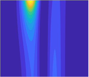
Figure 8 shows the contours of the linear periodic-wave-induced pore pressure and effective stresses inside the seabed. The effective stresses vanish at the water–seabed interface as required by the boundary conditions, and the amplitudes of the effective stresses increase with increasing soil depth. The effective horizontal normal stress, $\tau _{xx}$, and shear stress, $\tau _{xz}$, are smaller than the effective vertical normal stress, $\tau _{zz}$. Under the wave crest, the pressure reaches a maximum value at the water–seabed interface and damps with increasing soil depth, resulting in a negative vertical pressure gradient. Owing to this negative pressure gradient, the soil skeleton is compressed, and therefore a negative effective vertical normal stress (compression) is generated within the seabed. As the crest passes, the wave-induced pore pressure at the interface decreases on the interface and increases within the seabed. Consequently, the vertical pressure gradient increases and changes sign before the arrival of the wave trough. Therefore, a positive effective vertical normal stress (tension) is generated inside the seabed under the trough. The tendency of the effective horizontal effective stress is the same as that of the effective vertical normal stress, since $\tau _{xx}\propto \tau _{zz}$ in a shallow seabed according to (3.20). In addition, the shear stress, $\tau _{xz}$, is positive in the ascending phase and negative in the receding phase. Lastly, the linear wave-induced pore pressure and effective stresses are symmetric.

Figure 8. Contours of pore pressure and effective stresses inside a seabed: (a) the time history of the linear wave-induced dynamic water pressure at the water–seabed interface; (b) contours of the pore pressure $p$; (c) contours of the horizontal effective stress $\tau _{xx}$; (d) contours of the vertical effective stress $\tau _{zz}$; and (e) contours of the shear stress $\tau _{xz}$. The physical parameters used in the calculation are given in the caption of figure 7.

Figure 9 displays the time histories of dimensionless velocity components of the pore fluid, (3.17) and (3.26), and the soil skeleton, (3.16) and (3.24), at three different elevations, $Z=1.0$, 0.5 and 0, in which the left column shows the horizontal velocity components and the right column shows the vertical velocity components. For clarity, detailed vertical profiles of the velocity components at four different phases during the third wave period are also plotted in figure 10.

Figure 9. Time histories of linear wave-induced dimensionless velocity components at three different elevations, (a,b) $Z=1$, (c,d) $Z=0.5$ and (e, f) $Z=0$, within an unsaturated poroelastic seabed. Black solid lines, the pore fluid velocity components; blue solid lines, the soil skeleton velocity components;red solid lines, the velocity difference of the pore fluid and soil skeleton calculated by the present solutions; and red dashed lines, the velocity difference of the pore fluid and soil skeleton calculated by Liu et al. (Reference Liu, Park and Lara2007) for a rigid soil skeleton. The physical parameters used in the calculation are given in the caption of figure 7.

Figure 10. Vertical profiles of the dimensionless velocity components of the pore fluid, the soil skeleton and the seepage flow at four different phases: (a) the time history of the dynamic water pressure at the water–seabed interface; (b–e) the vertical profiles of the horizontal velocity components at $\varphi _1=-0.75$, $\varphi _2=-0.50$, $\varphi _3=-0.25$ and $\varphi _4=0$, respectively; and ( f–i) the vertical profiles of the vertical velocity components at $\varphi _1=-0.75$, $\varphi _2=-0.50$, $\varphi _3=-0.25$ and $\varphi _4=0$, respectively. Black solid lines, the pore fluid velocity components; blue solid lines, the soil skeleton velocity components; red solid lines, the differences of the pore fluid and soil skeleton velocities calculated by the present solutions; and red dashed lines, the difference of the pore fluid and soil skeleton velocities calculated by Liu et al. (Reference Liu, Park and Lara2007). The physical parameters used in the calculation are given in the caption of figure 7.

Since the shear modulus of the soil, $G$, equals the effective bulk modulus of elasticity of the pore fluid, $K$, under the present soil properties, the amplitudes of the velocity components of the soil skeleton at $Z=1.0$ and $Z=0.5$ are no longer negligible, compared with those of the pore fluid. At the bottom of the seabed, $Z=0$, the velocity components of the soil skeleton vanish, determined by the boundary conditions. The horizontal velocity component of the pore fluid is negative under the crest and positive under the trough. The horizontal velocity component of the soil skeleton shows similar features; however, it reverses its direction before the horizontal velocity component of the the pore fluid changes its sign. In the vertical direction, the vertical velocity components for the pore fluid and soil skeleton are positive in the receding phase and negative in the ascending phase, and the vertical velocity component of the soil skeleton also changes its direction before that of the pore fluid.

In addition, the vertical profiles of the velocity components are symmetric with respect to the wave crest and the wave trough, as shown in figure 10. The relative velocities between the pore fluid velocity and the soil skeleton velocity are compared in this figure as well. Recall that the soil skeleton in Liu et al. (Reference Liu, Park and Lara2007) is rigid, and therefore the relative velocities and the seepage flow velocities calculated in Liu et al. (Reference Liu, Park and Lara2007) are identical. The results show that the relative horizontal velocities are relatively small except near the bottom of the seabed, compared with the horizontal velocities of the pore fluid and soil skeleton. At the seabed bottom, the horizontal velocity component of the soil skeleton will be zero as required by the boundary condition, and therefore the relative horizontal velocity component is the same as the horizontal velocity component of the pore fluid. As can be seen from figure 10, both the amplitudes and phases of the relative velocity components in the present solution and the solution of Liu et al. (Reference Liu, Park and Lara2007) are different inside the seabed. This can be attributed to the fact that the pressure calculated from these two theories are different within the seabed (see figure 7), and $\boldsymbol {\nabla }{p} \propto \boldsymbol {u}_{{f}}-\boldsymbol {u}_{{s}}$, (2.12) and (2.13), is true from both theories.

In the poroelastic seabed model, the discharge volume of pore fluid, $n {\partial }{w_f}/ {\partial }{Z}$, is equal to the total compression volume of the soil skeleton, $ {\partial }{w_s}/ {\partial }{Z}$, and the pore fluid, $\tilde {G} {\partial }{p}/ {\partial }{t}$, based on (3.2) and (2.13). Under the present wave conditions and soil properties, the wave-induced vertical normal effective stress reaches up to 0.72 at the seabed bottom (see figure 8), and therefore, according to (2.10) and (2.11), the compression volume of the soil skeleton is considerable, compared with that of the pore fluid. However, in the rigid seabed model, the compression volume of the soil skeleton is assumed to be zero (Liu et al. Reference Liu, Park and Lara2007). Consequently, the various fluid velocities calculated from both theories are significantly different.

5.2. Solitary-wave-induced pore-pressure and soil responses

It is well known that the effective wavelength and wave period of a solitary wave can be expressed as (e.g. Dean & Dalrymple Reference Dean and Dalrymple1991)

(5.1a,b)\begin{equation} l^\prime_0=h^\prime\sqrt{\frac{4h^{\prime}}{3a^\prime_0}} {\quad{\rm and}\quad} T^\prime=\frac{l^\prime_0}{\sqrt{gh^\prime}}, \end{equation}

respectively, which have been used as the horizontal length scale and the time scale for the present problem. Recall that $a_0^\prime$ is the solitary-wave height and $h^\prime$ is the water depth. Correspondingly, the dimensionless dynamic water pressure at the water–seabed interface approximated by normalized free-surface elevation can be written as (Packwood & Peregrine Reference Packwood and Peregrine1980; Knowles & Yeh Reference Knowles and Yeh2018)

(5.2)\begin{equation} p_b={{\rm sech}}^2(x-Ct), \end{equation}

where $C$ is the dimensionless wave celerity, defined as $C=\sqrt {1+a^\prime _0/h^{\prime }}$, and $a^\prime _0/h^{\prime }$ measures the wave nonlinearity. Substituting the above expressions into (3.12), (3.16)–(3.18), (3.20), (3.21), (3.24) and (3.26), respectively, the dynamic responses inside the seabed are obtained. To illustrate various physical features, the solitary-wave conditions are set to be $h^\prime =30$ m and $a^\prime _0/h^{\prime }=0.2$ as an example.

In figure 11, the time histories of the wave-induced pore pressure are plotted at three different elevations in the seabed, $Z=1.0$, 0.5 and 0, respectively. For a solitary wave, the moving coordinate, $\varphi =x-Ct$, is used. The solitary-wave loading at the water–seabed interface ($Z=1$) is symmetric with respect to the wave crest ($\varphi =0$). However, the profiles become asymmetric at the mid-depth ($Z=0.5$) and the bottom of the seabed ($Z=0$), since the soil responses have a memory of the history of the spatial variation of the wave loading. There are also phase lags in the arrival of the maximum pore pressure. In addition, the width of the asymmetric pressure distribution becomes wider towards the bottom of the seabed. The width is defined as the time interval within which the pore pressure is larger than 1 % of the maximum pressure amplitude. Without considering the deformation of the soil skeleton, the phase lags are longer inside the seabed as well.

Figure 11. Time histories of the solitary-wave-induced dimensionless pore pressure within an unsaturated poroelastic seabed at three different elevations: (a) $Z=1$ on the seabed–water interface; (b) $Z=0.5$ at mid-depth of the seabed; and (c) $Z=0$ on the seabed bottom. Black solid lines, the present solution (3.12); and red dashed lines, the solution of Liu et al. (Reference Liu, Park and Lara2007) for a rigid soil skeleton. The following parameters are used for calculation: $\alpha =2.79$, $\beta =0.36$, $\kappa _1=3.33\kappa _2$ and $\tilde {\nu }=0.25$. These correspond to the physical conditions: $n=0.45$, $\nu =0.33$, $G=K=2\times {10^7}$ Pa, $k_s=1\times {10}^{-10}~\textrm {m}^2$, $\rho _f=1\times 10^3~\textrm {kg}~\textrm {m}^{-3}$, $v_f=1\times {10}^{-6}~\textrm {m}^2~\textrm {s}^{-1}$, $d^\prime =10~\textrm {m}$, $h^\prime =30$ m and ${a^\prime _0}/{h^\prime }=0.2$.

Figure 12 shows the contours of the solitary-wave-induced pore pressure and effective stresses within the seabed. As shown in the figure, the amplitudes of the effective stresses also increase with increasing soil depth. In the acceleration phase, the pressure inside the seabed damps with increasing soil depth, and therefore the soil is also compressed by the wave-induced pressure. After the wave crest, the dynamic water pressure at the interface decreases; however, due to the phase lag, the pressure within the seabed continues to increase. As a result, the pressure gradient changes sign from negative to positive, and a positive effective vertical normal stress is generated inside the seabed. Correspondingly, the effective shear stress changes sign in the opposite manner. Since the wave-induced pressure is relatively small at the seabed bottom, compared with the dynamic water pressure at the interface, the positive vertical pressure gradient in the deceleration phase is weak, and it takes a relatively long time to dissipate the wave-induced pressure and effective normal stresses.

Figure 12. Contours of pore pressure and effective stresses inside a seabed: (a) the time history of the solitary-wave-induced dynamic water pressure at the water–seabed interface; (b) contours of the pore pressure $p$; (c) contours of the horizontal effective stress $\tau _{xx}$; (d) contours of the vertical effective stress $\tau _{zz}$; and (e) contours of the shear stress $\tau _{xz}$. The physical parameters used in the calculation are given in the caption of figure 11.

Figure 13 further displays the time histories of dimensionless velocity components of the pore fluid and the soil skeleton at three different elevations, $Z=1.0$, 0.5 and 0. The vertical profiles of the velocity components at five different phases are also plotted in figure 14. In the seabed, the horizontal velocity component of the pore fluid reverses its direction, first from positive to negative and then reverses it again from negative to positive after the horizontal pressure gradient changes its sign. The horizontal soil skeleton velocity behaves similarly, while its value is smaller in the acceleration phase and larger in the deceleration phase. However, the vertical velocity components show different features. Both the vertical velocity components of the pore fluid and soil skeleton simply reverse their directions from positive to negative before the vertical pressure gradient changes its sign with increasing $\varphi$. The relative velocities between the pore fluid velocity and the soil skeleton velocity are compared in these figures as well. Owing to the wave-induced soil deformation within the seabed, the difference between the present solution and the solution of (Liu et al. Reference Liu, Park and Lara2007) is also obvious under a solitary wave.

Figure 13. Time histories of solitary-wave-induced dimensionless velocity components at three different elevations, (a,b) $Z=1$, (c,d) $Z=0.5$ and (e, f) $Z=0$, within an unsaturated poroelastic seabed. Black solid lines, the pore fluid velocity components; blue solid lines, the soil skeleton velocity components; red solid lines, the velocity difference of the pore fluid and soil skeleton calculated by the present solutions; and red dashed lines, the velocity difference of the pore fluid and soil skeleton calculated by Liu et al. (Reference Liu, Park and Lara2007) for a rigid soil skeleton. The physical parameters used in the calculation are given in the caption of figure 11.

Figure 14. Vertical profiles of the dimensionless velocity components of the pore fluid, the soil skeleton and the seepage flow at five different phases: (a) the time history of the dynamic water pressure at the water–seabed interface; (b–f) the vertical profiles of the horizontal velocity components at $\varphi _1=-2$, $\varphi _2=-1$, $\varphi _3=0$, $\varphi _4=1$ and $\varphi _5=2$, respectively; and (g–k) the vertical profiles of the vertical velocity components at $\varphi _1=-2$, $\varphi _2=-1$, $\varphi _3=0$, $\varphi _4=1$ and $\varphi _5=2$, respectively. Black solid lines, the pore fluid velocity components; blue solid lines, the soil skeleton velocity components; red solid lines, the differences of the pore fluid and soil skeleton velocities calculated by the present solutions; and red dashed lines, the difference of the pore fluid and soil skeleton velocities calculated by Liu et al. (Reference Liu, Park and Lara2007). The physical parameters used in the calculation are given in the caption of figure 11.

5.3. Bore-induced pore-pressure and soil responses

According to Packwood & Peregrine (Reference Packwood and Peregrine1980), the horizontal length scale and the time scale for a bore can be represented by (5.1a,b) as well. Thus, the bore-induced dimensionless dynamic water pressure at the water–seabed interface can be expressed as (Liu et al. Reference Liu, Park and Lara2007)

(5.3)\begin{equation} p_b=\tfrac{1}{2} [1-{{\rm tanh}}(x-Ct)], \end{equation}

where $C$ is the dimensionless bore velocity. Substituting (5.3) into the leading-order solutions for the pore pressure (3.12), the effective stresses (3.18), (3.20) and (3.21) and the velocity components of the pore fluid and soil skeleton (3.16), (3.17), (3.24) and (3.26), respectively, various features of seabed response under a bore can be obtained.

To quantify the results, the same set of physical parameters as employed in the previous subsection is used herein. In figure 15, time histories of the dimensionless pore pressure at three elevations inside the seabed, $Z=1.0$, 0.5 and 0, respectively, are displayed. The moving coordinate, $\varphi =x-Ct$, is adopted for convenience. Under the present conditions, the diffusion depth of the pore pressure, $1/\alpha$, is 0.36. Below the diffusion depth, the vertical pressure gradient is small, and $p\rightarrow {\beta {p_b}}$. Therefore, the pore pressure at $Z=0.5$ and $Z=0$ starts to grow in parallel to the wave loading (see figure 15). Meanwhile, the diffusion time scale, $\alpha ^2$, decreases, when $G\rightarrow {\infty }$. Thus, compared with the solution of Liu et al. (Reference Liu, Park and Lara2007), the present poroelastic solution starts to increase earlier and takes a longer time to reach the maximum value.

Figure 15. Time histories of the bore-induced dimensionless pore pressure at three different elevations inside the seabed: (a) $Z=1$, (b) $Z=0.5$ and (c) $Z=0$.Black solid lines, the present solution; and red dashed lines, the solution of Liu et al. (Reference Liu, Park and Lara2007). The physical parameters used in the calculation are given in the caption of figure 11.

The contours of the pore pressure and the effective stresses are displayed in figure 16. The results also show that the normal effective stresses, $\tau _{xx}$ and $\tau _{zz}$, have the same sign, while the shear stress has the opposite sign. As compared to those under a solitary wave, the bore-induced responses correspond to those during the acceleration phase of the solitary wave.

Figure 16. Contours of the pore pressure and effective stresses under a bore: (a) the time history of the dynamic water pressure at the water–seabed interface; (b) contours of the pore pressure $p$; (c) contours of the horizontal effective stress $\tau _{xx}$; (d) contours of the vertical effective stress $\tau _{zz}$; and (e) contours of the shear stress $\tau _{xz}$. The physical parameters used in the calculation are given in the caption of figure 11.

In figure 17, time histories of the velocity components for the pore fluid and soil skeleton at three different elevations are shown. The vertical profiles of these velocity components in the seabed at five different phases, $\varphi =-2,-1,0,1$ and 2, are plotted in figure 18. As shown in these figures, the horizontal velocity component for the pore fluid and soil skeleton in the seabed reverses its direction from negative to positive as $\varphi$ increases. However, the vertical velocity component first decreases, then increases to zero. Relatively, the vertical soil skeleton velocity components are small (see figure 17). The differences of the velocities of the pore fluid and the soil skeleton are displayed in these figures as well. Since the pore pressure speeds up to increase at first and then slows down to be a constant (see figure 15), the horizontal relative velocity component first increases, and then gradually decreases to zero inside the seabed. Correspondingly, the vertical relative velocity component behaves in the opposite manner. At the seabed bottom, the vertical relative velocity component is zero, as required by the condition of no vertical flow.

Figure 17. Time histories of the bore-induced dimensionless velocity components for the pore fluid and soil skeleton at three different elevations: (a,b) $Z=1$, (c,d) $Z=0.5$ and (e, f) $Z=0$. Black solid lines, the pore fluid velocity components; blue solid lines, the soil skeleton velocity components; red solid lines, the relative velocity between pore fluid and soil skeleton calculated by the present solutions; and red dashed lines, the relative velocity between pore fluid and soil skeleton calculated by Liu et al. (Reference Liu, Park and Lara2007). The physical parameters used in the calculation are given in the caption of figure 11.

Figure 18. Vertical profiles of the dimensionless velocity components of the pore fluid and the soil skeleton in the seabed at five different phases: (a) the time history of the dynamic water pressure at the water–seabed interface; (b–f) the vertical profiles of the horizontal velocity components at $\varphi _1=-2$, $\varphi _2=-1$, $\varphi _3=0$, $\varphi _4=1$ and $\varphi _5=2$, respectively; and (g–k) the vertical profiles of the vertical velocity components at $\varphi _1=-2$, $\varphi _2=-1$, $\varphi _3=0$, $\varphi _4=1$ and $\varphi _5=2$, respectively. Black solid lines, the pore fluid velocity components; blue solid lines, the soil skeleton velocity components; red solid lines, the relative velocity between pore fluid and soil skeleton calculated by the present solutions; and red dashed lines, the relative velocity between pore fluid and soil skeleton calculated by Liu et al. (Reference Liu, Park and Lara2007). The physical parameters used in the calculation are given in the caption of figure 11.

The comparisons of the present solution with the solution of Liu et al. (Reference Liu, Park and Lara2007) show that the soil skeleton deformation has some influence on the damping rate and the phase shift of the seepage velocity under a bore. Under the bore front, the soil is compressed as shown in figure 16. The vertical velocity component of the soil skeleton is negative and damps with the increase of the soil depth, which prevents the fluid from flowing into the seabed. Thus, the difference of the vertical relative velocities of these two solutions decreases with increasing soil depth. The results also show that the difference of the relative velocities of the present solution and the solution of Liu et al. (Reference Liu, Park and Lara2007) increases with increasing soil depth in the horizontal direction.

6.1. Transient wave-induced shear failure potential in the seabed

Using the experimental conditions listed in table 1, the stress angle inside the seabed given by Anderson et al. (Reference Anderson, Cox, Mieras, Puleo and Hsu2017) can be calculated and is shown in figure 19. The stress angle increases during the acceleration phase and has larger values near the bottom of the seabed. The maximum stress angle in the entire wave cycle, $\phi _{{max}}$, is $29.8^{\circ }$, which is smaller than the internal friction angle of the prescribed soil properties ($\phi _c=30.1^{\circ }$), suggesting that shear failure is unlikely to occur inside the seabed for this experimental set-up.

Figure 19. (a) Time history of the phase-averaged dynamic water pressure at the water–seabed interface measured by Anderson et al. (Reference Anderson, Cox, Mieras, Puleo and Hsu2017). (b) The contour map of the stress angle inside the seabed. The stress angle achieves its maximum, $29.8^\circ$, at the seabed bottom when $t=0.525$. The physical parameters are given in table 1.

Under the linear wave conditions and soil properties presented in § 5, the stress angles within the seabed are calculated from (6.5). Figure 20 shows the contour map of the stress angle during the second and third wave periods. Owing to the wave-induced effective stresses, the stress angles inside the seabed increase in both the deceleration and acceleration phases. Since the wave-induced effective vertical normal stress is positive (tension) in the deceleration phase and negative (compression) in the acceleration phase (see figure 8), the effective weight of the soil decreases in the deceleration phase and increases in the acceleration phase. Recall that the wave-induced effective shear stress is symmetric, and therefore the stress angle increases more in the deceleration phase. The results show that the maximum stress angle under the linear wave is $31.6^\circ$, which is around the critical value, $31^\circ$. As shown in figure 20, shear failure may occur near the water–seabed interface in the deceleration phase, which is consistent with Ren et al. (Reference Ren, Xu, Xu, Zhao and Wang2020).

Figure 20. (a) The time history of the dynamic water pressure at the water–seabed interface under a linear wave with $T^\prime =15~\textrm {s}$, $h^\prime =30$ m and $a_0^\prime /h^\prime =0.10$. (b) The colour map of the stress angle inside the seabed during linear wave propagation. The stress angle achieves the maximum, $31.6^\circ$, at the water–seabed interface in the deceleration phase, and the red line indicates the contour of $\phi =\phi _c$. The physical parameters used in the calculation are given in the caption of figure 7.

Combining the wave-induced effective stresses calculated in § 5 with the effective stresses at the quiescent state, the stress angle under the solitary wave can be obtained, which is shown in figure 21(b). The stress angle decreases towards the bottom of the soil bed and reaches its maximum in the deceleration phase at the water–seabed interface. Under the present solitary-wave conditions (i.e. $a^\prime _0/h^\prime =0.2$ and $h^\prime =30$ m) and soil properties, the maximum stress angle is estimated as $20.7^\circ$, and it is not large enough to cause shear failure, which is $\phi _c=31^\circ$. However, if $a^\prime _0/h^\prime$ increases to 0.4, as discussed in Packwood & Peregrine (Reference Packwood and Peregrine1980) with the same seabed properties, the maximum of $\phi$ increases drastically to $90^\circ$. Clearly, the criterion of (6.1) will be satisfied. Figure 22 shows the contour map of the stress angle for this large solitary wave. The results indicate that the shear failure depth reaches up to 20 % of the seabed thickness. Recall that solitary-wave-induced effective vertical normal stress is also negative (compression) in the acceleration phase and positive (tension) in the deceleration phase, and therefore shear failure is more likely to occur in the deceleration phase. As suggested by Yamamoto (Reference Yamamoto1978), the total effective stresses will vanish, and the sand will be liquefied, when the stress angle reaches $90^\circ$. As shown in figure 22, under such a large solitary wave, momentary liquefaction may occur near the water–seabed interface as well, and it starts after the beginning of shear failure and ends before the end of shear failure. Note that the poroelastic theory is no longer valid once shear failure occurs. To investigate the liquefaction potential and related processes within the seabed, a poroelastoplastic model is further required (Young et al. Reference Young, White, Xiao and Borja2009).

Figure 21. (a) The time history of the dynamic water pressure at the water–seabed interface under a solitary wave with $a_0^\prime /h^\prime =0.2$ and $h^\prime =30$ m. (b) The colour map of the stress angle inside the seabed under a solitary wave. The stress angle achieves the maximum, $20.7^\circ$, at the water–seabed interface when $\varphi =-0.94$. The physical parameters used in the calculation are given in the caption of figure 11.

Figure 22. (a) The time history of the dynamic water pressure at the water–seabed interface under a solitary wave with $a^\prime _0/h^\prime =0.4$ and $h^\prime =30~\textrm {m}$. (b) The colour map of the stress angle inside the seabed. The red line indicates the contour of $\phi =\phi _c$, and the black line indicates the contour of $\phi =90^\circ$. The other parameters used in the calculation are consistent with those given in the caption of figure 11.

Using the wave conditions and seabed properties presented in § 5, the stress angles under the bore are calculated and displayed in figure 23. The stress angle increases from the water–seabed interface towards the bottom of the seabed. The maximum value, $19.98^\circ$, appears at the bottom of the seabed when $\varphi =0.04$. Clearly, shear failure does not occur within the seabed for this case, since the internal friction angle of the soil is $31^\circ$. Note that, under a bore, the pore pressure is always in the acceleration phase and the effective normal stress is always in compression, which create a less favourable condition for shear failure. However, the effective shear stress also contributes to the increase of stress angle, i.e. see (6.4). Thus, the potential of shear failure will increase if the bore strength is increased. For example, if $a^\prime _0/h^\prime$ is increased to 1, which is most likely a breaking bore, the maximum stress angle increases to $24.9^\circ$, which is still not large enough to cause shear failure. However, if $a^\prime _0/h^\prime$ is further increased to 2, the maximum stress angle increases to $36.3^\circ$, and shear failure occurs near the bottom of the seabed. Note that such a violent (turbulent) bore could occur in extreme conditions, such as tsunamis; however, the frictional stress on the water–seabed interface becomes significant and needs to be considered. This is beyond the scope of the present study.

Figure 23. (a) History of the dynamic water pressure at the water–seabed interface under a bore. $(b)$ Contours of the stress angle inside the seabed under a bore. The stress angle reaches the maximum $19.98^\circ$ at the bottom of the seabed when $\varphi =0.04$. The physical parameters used in the calculation are given in the caption of figure 11.

6.2. Effects of soil properties on shear failure

The analytical solutions for the wave-induced effective stresses (i.e. (3.18), (3.20) and (3.21)) depend on the soil properties, such as the degree of saturation $S_r$, the shear modulus $G$ and the permeability $k_s$, suggesting that the shear failure potential of the seabed is affected by the soil properties as well. In this section, as an illustration, the effects of these three parameters ($S_r$, $G$ and $k_s$) on the shear failure are investigated under solitary waves with $a^\prime _0/h^\prime =0.4$ and $h^\prime =30$ m.

First, the effects of the degree of saturation, $S_r$, on shear failure are investigated for a highly saturated seabed with $S_r$ between 0.94 and 0.998 (Sumer Reference Sumer2014). The corresponding bulk modulus of elasticity of the pore fluid, $K$, varies from $4.9\times {10^6}$ Pa to $1.38\times {10^8}$ Pa. The other soil parameters remain the same as those presented in § 5. Using (6.5), the stress angle $\phi$ inside the seabed can be calculated. For a specified elevation $Z$, shear failure does not occur if the maximum of $\phi$, denoted by $\phi _{{max}}(S_{r},Z)$, is smaller than the critical value $\phi _c$, namely $\phi _{{max}}(S_{r},Z)<\phi _c$. Therefore, the values of $\phi _{{max}}(S_{r},Z)$ in the parameter space $0.94< S_r<0.998$ and $0< Z<1$ are numerically calculated and displayed in figure 24. In figure 24, the red line indicates the contour of $\phi _{{max}}(S_{r},Z)=\phi _c$. The region below the red line is called the stable zone and the region above is called the shear failure zone in this paper.

Figure 24. The contour map of the maximum stress angle $\phi _{{max}}(S_r,Z)$ induced by a solitary wave with $a_0^\prime /h^\prime =0.4$ and $h^\prime =30$ m (the red line indicates the contour of $\phi _{{max}}(S_{r},Z)=\phi _c$). Shear failure occurs when $S_r\leq {0.9943}$. The physical parameters used in the calculation are given in the caption of figure 11.

As shown in figure 24, $\phi _{{max}}(S_{r},Z)$ is sensitive to the change of saturation. Shear failure occurs near the water–seabed interface when the saturation degree $S_r$ is smaller than 0.9943, and the shear failure depth decreases gradually when $S_r$ increases from 0.94 to 0.9943. For a seabed with large saturation degree, the ratio between $G$ and $K$ measured by $\tilde {G}$ is relatively small; for example, when $S_r=0.998$, $\tilde {G}=0.065$. Accordingly, the dimensionless parameter $\beta$ is relatively large, indicating that the wave-induced effective stresses are weak inside the seabed. Thus, it is difficult for shear failure to happen in this situation. When $S_r$ decreases, the diffusion depth of the wave-induced pressure decreases as well and the effective stresses increase rapidly in the diffusion region. Therefore, the maximum stress angle quickly damps to a small value with increasing soil depth.

Besides the shear failure potential, information on the initiation and duration of shear failure are also important. Figure 25 shows the interface of the shear failure zone and the stable zone under four different degrees of saturation degree, i.e. $S_r=0.96$, 0.98, 0.99 and 0.993. Under the solitary wave, shear failure starts earlier and ends later with decreasing degree of saturation.

Figure 25. (a) The time history of the dynamic water pressure at the water–seabed interface under a solitary wave with $a^\prime _0/h^\prime =0.4$ and $h^\prime =30$ m. (b) The interface between the shear failure zone and the stable zone under the conditions of $S_r=0.96$, 0.98, 0.99 and 0.993. The parameters used in the calculation are given in the caption of figure 11.

For dense sand, the shear modulus of the seabed, $G$, is of the order of magnitude of $O(10^8~\textrm {Pa})$, but it reduces to $O(10^6~\textrm {Pa})$ for loose sand (Yamamoto Reference Yamamoto1978; Zhai et al. Reference Zhai, He, Zhao, Zhang, Jeng and Li2018). The effects of shear modulus on shear failure are studied for $2\times {10^6}~\textrm {Pa} < G < 4.4\times {10^8}~\textrm {Pa}$. Using the soil properties presented in § 5, the dimensionless parameter $\tilde {G}$ varies from 0.045 to 10. By numerical integration, the maximum stress angle, $\phi _{{max}}(\tilde {G},Z)$, can be calculated and is displayed in figure 26.

Figure 26. The contour map of the maximum stress angle, $\phi _{{max}}(\tilde {G},Z)$, induced by a solitary wave with $a^\prime _0/h^\prime =0.4$ and $h^\prime =30$ m. The red line indicates the contour of $\phi _{{max}}(\tilde {G},Z)=\phi _c$, and shear failure occurs when $\tilde {G} \geq 0.068$. In the calculation, the shear modulus varies between $2\times {10^6}$ Pa and $4.4\times {10^8}$ Pa, and the other physical parameters used in the calculation are given in the caption of figure 11.

In figure 26, the red line denotes the contour of $\phi _{{max}}(\tilde {G},Z)=\phi _c$. Shear failure occurs when $\tilde {G}$ is larger than 0.068. Near the water–seabed interface, the maximum stress angle increases rapidly with increasing $\tilde {G}$. For a loose seabed, $\tilde {G}$ is small, and the dimensionless parameter $\beta$ approaches 1. Similar to the scenario of a large degree of saturation, the wave-induced effective vertical normal stress $\tau _{zz}$ is small. Physically, this means that most of the wave loading is balanced by the pore fluid, as the soil skeleton is easier to compress than the pore fluid. Hence shear failure is unlikely to occur inside the seabed in this case. However, for dense seabed with relatively large $\tilde {G}$, the dimensionless parameter $\beta$ becomes close to 0. For example, when $\tilde {G}=10$, then $\beta =0.02$. Meanwhile, the dimensionless parameter $\alpha$, which can be viewed as the inverse of the diffusion distance for the pore pressure, is insensitive to the change of shear modulus when $\tilde {G}$ is relatively large. For example, $\alpha =2.72$ when $\tilde {G}=5$, and $\alpha =2.69$ when $\tilde {G}=10$. Based on (3.18), $\tau _{zz}$ varies over a wide range in this scenario, and the wave-induced tension stress in the deceleration phase is relatively large. Consequently, the shear failure potential increases.

Figure 27 further shows the interface between the shear failure zone and the stable zone under four different shear modulus conditions, i.e. $\tilde {G}=0.1$, 0.3, 1.0 and 10. Shear failure starts earlier and ends later with increasing shear modulus.

Figure 27. (a) The time history of the dynamic water pressure at the water–seabed interface under a solitary wave with $a^\prime _0/h^\prime =0.4$ and $h^\prime =30$ m (b) The interface between the shear failure zone and the stable zone under the conditions of $\tilde {G}=0.1$, 0.3, 1.0 and 10. The other parameters used in the calculation are given in the caption of figure 11.

Since the soil permeability $k_s$ is of the order of magnitude of $O(10^{-11}~\textrm {m}^2)$ for fine sandy seabed and $O(10^{-9}~\textrm {m}^2)$ for coarse sandy seabed (Hsu & Jeng Reference Hsu and Jeng1994), the effects of the soil permeability on shear failure are studied for $10^{-11}~\textrm {m}^2< k_s <10^{-9}~\textrm {m}^2$. The corresponding dimensionless parameter $\kappa _2^2$ varies from $2.1\times {10^{-4}}$ to $2.1\times {10^{-2}}$. The contour map of the maximum stress angle $\phi _{{max}}({\kappa _2^2},Z)$ is produced and displayed in figure 28. In the figure, the red line represents the contour of $\phi _{{max}}(\kappa _2^2,Z)=\phi _c$, separating the shear failure zone and the stable zone. As shown in figure 28, shear failure always occurs near the water–seabed interface. Meanwhile, the shear failure depth is affected by the soil permeability, because the diffusion distance of $p$ measured by $1/\alpha$ increases with increasing $k_s$.

Figure 28. The contour map of the maximum stress angle, $\phi _{{max}}(\kappa _2^2,Z)$, induced by a solitary wave with $a_0^\prime /h^\prime =0.4$ and $h^\prime =30$ m; the red line indicates the contour of $\phi _{\textrm {max}}(\kappa _2^2,Z)=\phi _c$. In the calculation, the soil permeability varies from $10^{-11}~\textrm {m}^2$ to $10^{-9}~\textrm {m}^2$, and the other physical parameters used in the calculation are given in the caption of figure 11.

Figure 29 further shows the interface between the shear failure zone and stable zone under three different permeability conditions, $\kappa _2^2=2\times {10^{-3}}$, $7\times {10^{-3}}$ and $2\times {10^{-2}}$. Shear failure starts early and lasts for a short time when $\kappa _2^2$ is relatively large. This is because it is more difficult for the pore fluid to drain out to dissipate the wave-induced pore pressure for the seabed with small permeability.

Figure 29. (a) The time history of the dynamic water pressure at the water–seabed interface under a solitary wave with $a^\prime _0/h^\prime =0.4$ and $h^\prime =30$ m. (b) The interface between the shear failure zone and the stable zone under soil permeability conditions of $\kappa _2^2=2\times {10^{-3}}$, $7\times {10^{-3}}$ and $2\times {10^{-2}}$. The parameters used in the calculation are given in the caption of figure 11.