


1. Introduction
Active particles, e.g. micromotors and motile micro-organisms, can harvest energy from the environment for self-propulsion, known as active Brownian motion (Schweitzer Reference Schweitzer2003; Romanczuk et al. Reference Romanczuk, Bär, Ebeling, Lindner and Schimansky-Geier2012), which is fundamentally different from the pure translational Brownian motion of passive particles without swimming ability. The transport mechanism of active particles is significant for various biological, environmental and chemical applications, such as algae cultivation (Posten Reference Posten2009; Acién et al. Reference Acién, Molina, Reis, Torzillo, Zittelli, Sepúlveda and Masojídek2017), remedies for harmful algal blooms (Durham & Stocker Reference Durham and Stocker2012; Liu et al. Reference Liu, Liu, Johnson, Yi and Huang2012), bioreactors for biofuels (Chisti Reference Chisti2007; Bees & Croze Reference Bees and Croze2014) and cargo transport (Yasa et al. Reference Yasa, Erkoc, Alapan and Sitti2018; Xiao, Wei & Wang Reference Xiao, Wei and Wang2019).
Active particles often swim in confined environments, e.g. synthetic microswimmers in a micro-channel, or bacteria in the digestive tract. Complicated interactions of active particles with physical boundaries play a key role in the transport process and result in rich phenomena, such as wall scattering (Drescher et al. Reference Drescher, Dunkel, Cisneros, Ganguly and Goldstein2011; Kantsler et al. Reference Kantsler, Dunkel, Polin and Goldstein2013), circular trajectories (Berg & Turner Reference Berg and Turner1990; Lauga et al. Reference Lauga, DiLuzio, Whitesides and Stone2006), shear-induced trapping (Rusconi, Guasto & Stocker Reference Rusconi, Guasto and Stocker2014) and rheotaxis (Uspal et al. Reference Uspal, Popescu, Dietrich and Tasinkevych2015; Brosseau et al. Reference Brosseau, Usabiaga, Lushi, Wu, Ristroph, Zhang, Ward and Shelley2019; Mathijssen et al. Reference Mathijssen, Figueroa-Morales, Junot, Clément, Lindner and Zöttl2019). As one of the most well-known phenomena, micro-organisms such as spermatozoa and Escherichia coli are found to accumulate near the surfaces of confined domains (Rothschild Reference Rothschild1963; Berke et al. Reference Berke, Turner, Berg and Lauga2008). To explain this accumulation feature, many theoretical models have been proposed, such as the far-field and near-field hydrodynamic models (Berke et al. Reference Berke, Turner, Berg and Lauga2008; Li & Tang Reference Li and Tang2009; Spagnolie & Lauga Reference Spagnolie and Lauga2012; Sipos et al. Reference Sipos, Nagy, Di Leonardo and Galajda2015) and steric models considering inter-molecular forces like the van der Waals force (Li, Tam & Tang Reference Li, Tam and Tang2008; Costanzo et al. Reference Costanzo, Di Leonardo, Ruocco and Angelani2012; Chilukuri, Collins & Underhill Reference Chilukuri, Collins and Underhill2015; Contino et al. Reference Contino, Lushi, Tuval, Kantsler and Polin2015). Besides, many researchers have imposed a mathematically simple Robin boundary condition (the third type) for the probability density function (p.d.f.) of active particles in the position–orientation space (Enculescu & Stark Reference Enculescu and Stark2011; Elgeti & Gompper Reference Elgeti and Gompper2013; Ezhilan & Saintillan Reference Ezhilan and Saintillan2015; Alonso-Matilla, Chakrabarti & Saintillan Reference Alonso-Matilla, Chakrabarti and Saintillan2019; Jiang & Chen Reference Jiang and Chen2019a; Berlyand et al. Reference Berlyand, Jabin, Potomkin and Ratajczyk2020; Peng & Brady Reference Peng and Brady2020). Using this no-penetration condition for the probability flux at the boundaries, the wall accumulation phenomenon can be readily realised in numerical simulations (Bearon & Hazel Reference Bearon and Hazel2015; Ezhilan & Saintillan Reference Ezhilan and Saintillan2015; Nili et al. Reference Nili, Kheyri, Abazari, Fahimniya and Naji2017).
Because of the complex behaviours of active particles at the microscale, the transport characteristics at the macroscale have attracted practical attention. From a microscopic viewpoint, a high-dimensional Smoluchowski equation can be used to describe the transport process of swimmers in the position–orientation space, i.e. the phase space (Doi & Edwards Reference Doi and Edwards1988). The computational expense of such a microscopic model is potentially huge, even for some special applications (Zeng & Pedley Reference Zeng and Pedley2018). To characterise the effective transport process only in the position space (at the macroscale), simple macro-transport models have been proposed, by homogenising the fast- and small-scale swimming processes. The well-known model, the P–K model, proposed by Pedley & Kessler (Reference Pedley and Kessler1990, Reference Pedley and Kessler1992), uses a Fokker–Planck equation for the local p.d.f. of the swimming direction at each point in the position space and the active drift vector and the active translational dispersivity tensor are calculated based on the local p.d.f. associated with a correlation time coefficient. Another known model, called the GTD model, uses the generalised Taylor dispersion theory (Frankel & Brenner Reference Frankel and Brenner1989; Hill & Bees Reference Hill and Bees2002; Hill & Pedley Reference Hill and Pedley2005; Bearon, Hazel & Thorn Reference Bearon, Hazel and Thorn2011) to calculate the translational dispersivity tensor and gives some corrections for the P–K model for flows with strong shear rates. Although these two models are widely applied in current studies (Croze, Bearon & Bees Reference Croze, Bearon and Bees2017; Fung, Bearon & Hwang Reference Fung, Bearon and Hwang2020), they are only valid when the swimming scale is much smaller than the length scale of the confined environments (Bearon et al. Reference Bearon, Hazel and Thorn2011).
Furthermore, for active particles dispersing in confined flows, such as the common Poiseuille flow and Couette flow, the one-dimensional (1-D) macro-transport process in the longitudinal direction is of particular interest. The pioneering work by Bees & Croze (Reference Bees and Croze2010) introduced the P–K model for highly concentrated suspensions of gyrotactic swimmers in a vertical downwelling pipe flow. They derived the overall drift and dispersivity in the longitudinal direction based on the moment method by Aris (Reference Aris1956). In addition to the P–K model, Bearon, Bees & Croze (Reference Bearon, Bees and Croze2012) and Croze et al. (Reference Croze, Sardina, Ahmed, Bees and Brandt2013, Reference Croze, Bearon and Bees2017) applied the GTD model and gave more accurate results for the drift and dispersivity. However, these results may fail when the separate-length-scale requirement of the P–K model and GTD model is not satisfied, e.g. when the length scale of the confined section is comparable to that of the swimming, or the boundary effect cannot be neglected (Bearon et al. Reference Bearon, Hazel and Thorn2011). Recently, Jiang & Chen (Reference Jiang and Chen2019a, Reference Jiang and Chen2020) constructed a more integrated average approach also based on the GTD theory and analytically derived the overall drift and dispersivity for very dilute suspensions. This method gets rid of the separate-length-scale requirement of the P–K and GTD models, and thus is adaptable for wide applications. Jiang & Chen (Reference Jiang and Chen2019a) also considered the influence of wall accumulation on the dispersion process by introducing the Robin boundary condition for the p.d.f. (Elgeti & Gompper Reference Elgeti and Gompper2013; Bearon & Hazel Reference Bearon and Hazel2015; Ezhilan & Saintillan Reference Ezhilan and Saintillan2015). Peng & Brady (Reference Peng and Brady2020) analysed the accumulation effect on the upstream swimming (drift) based on an orientation-moment expansion method (Saintillan & Shelley Reference Saintillan and Shelley2013) and performed comparisons with the result by Brownian dynamics simulation.
The above studies on the dispersion process of active particles in confined flows mainly focused on the long-time asymptotic characteristics. However, little analytical work has been done to address the transient process. In fact, for active particles in unbounded position space, e.g. particles swim freely in a two-dimensional (2-D) confined thin film or a three-dimensional (3-D) space, abundant studies have investigated the transient diffusion process before the long-time diffusion limit (Howse et al. Reference Howse, Jones, Ryan, Gough, Vafabakhsh and Golestanian2007; ten Hagen, van Teeffelen & Löwen Reference ten Hagen, van Teeffelen and Löwen2011a; ten Hagen, Wittkowski & Löwen Reference ten Hagen, Wittkowski and Löwen2011b; Zheng et al. Reference Zheng, ten Hagen, Kaiser, Wu, Cui, Silber-Li and Löwen2013; Sandoval et al. Reference Sandoval, Marath, Subramanian and Lauga2014; Apaza & Sandoval Reference Apaza and Sandoval2020). Three basis stages are found in the temporal evolution of the mean squared displacement ( $\mathrm {MSD}$) of active particles with rotational-diffusion motions: diffusive at the short time scale (
 $\mathrm {MSD} \sim t$,
  $t$ is the time), ballistic during the intermediate time scales (
 $\mathrm {MSD} \sim t^2$) and finally again diffusive at the long time scale (
 $\mathrm {MSD} \sim t$) but with an enhanced dispersivity (Bechinger et al. Reference Bechinger, Di Leonardo, Löwen, Reichhardt, Volpe and Volpe2016). Because of the simplicity of the transport problem in a free space, the
  $\mathrm {MSD}$ of active particles can be theoretically derived, even for the case with a simple shear background flow (ten Hagen et al. Reference ten Hagen, Wittkowski and Löwen2011b; Sandoval et al. Reference Sandoval, Marath, Subramanian and Lauga2014). This anomalous diffusion (super-diffusion or sub-diffusion) process can be further analysed using non-Gaussian statistics, such as skewness and kurtosis (ten Hagen et al. Reference ten Hagen, van Teeffelen and Löwen2011a; Zheng et al. Reference Zheng, ten Hagen, Kaiser, Wu, Cui, Silber-Li and Löwen2013).
However, for confined flows, the boundaries tremendously increase the complexity of the transport problem of active particles, especially considering complicated swimming behaviours near boundaries such as the wall accumulation effect. To the best of our knowledge, only a few numerical studies, mainly using the Brownian dynamics simulation method, have addressed the transient active dispersion process in confined flows. Croze et al. (Reference Croze, Sardina, Ahmed, Bees and Brandt2013) investigated the dispersion of swimming algae in laminar and turbulent channel flows. The temporal evolution of the drift, effective diffusivity and skewness was calculated statistically. Chilukuri et al. (Reference Chilukuri, Collins and Underhill2015) also calculate these dispersion characteristics using a simplified interaction model (Chilukuri, Collins & Underhill Reference Chilukuri, Collins and Underhill2014) considering the influence of hydrodynamic interactions for wall accumulation. Apaza & Sandoval (Reference Apaza and Sandoval2016) focused on the hydrodynamic effects on the transient scale of the  $\mathrm {MSD}$. Other studies (Ghosh et al. Reference Ghosh, Misko, Marchesoni and Nori2013; Ao et al. Reference Ao, Ghosh, Li, Schmid, Hänggi and Marchesoni2014; Yariv & Schnitzer Reference Yariv and Schnitzer2014; Sandoval & Dagdug Reference Sandoval and Dagdug2014; Makhnovskii Reference Makhnovskii2019) have experimentally and numerically investigated the transient active dispersion process in a corrugated channel without background flow, considering the application of sorting particles by their self-propelled speeds. Additionally, it is of considerable interest to systematically compare the transient active dispersion process with the classic dispersion of passive particles (Lighthill Reference Lighthill1966; Foister & van de Ven Reference Foister and van de Ven1980; Latini & Bernoff Reference Latini and Bernoff2001; Camassa, Lin & McLaughlin Reference Camassa, Lin and McLaughlin2010; Vedel, Hovad & Bruus Reference Vedel, Hovad and Bruus2014; Taghizadeh, Valdés-Parada & Wood Reference Taghizadeh, Valdés-Parada and Wood2020), to capture the difference in approaching the Taylor dispersion regime (Chatwin Reference Chatwin1970; Wu & Chen Reference Wu and Chen2014; Li et al. Reference Li, Jiang, Wang, Guo, Li and Chen2018).
This work is to make a semi-analytical attempt to investigate the transient dispersion process of active particles in confined flows. Based on the GTD theory used in our previous studies (Jiang & Chen Reference Jiang and Chen2019a), we introduce the biorthogonal expansion method (Brezinski Reference Brezinski1991) to calculate the temporal evolution of moments of the cross-sectional mean concentration distribution, and then the basic dispersion characteristics, such as the local distribution in the confined-section–orientation space, the drift, dispersivity and skewness, can be obtained and analysed in the initial transient stage. The biorthogonal expansion method is often used to study the rheology of suspensions of particles (Strand, Kim & Karrila Reference Strand, Kim and Karrila1987; Nambiar et al. Reference Nambiar, Phanikanth, Nott and Subramanian2019). As an extension of the classic integral transform method with orthogonal bases for passive transport problems, the biorthogonal expansion method can solve the difficulty caused by the effect of the self-propulsion for the active transport problems. The auxiliary eigenvalue problem for the moments of distributions is solved by the Galerkin method with function series constructed for specific boundary conditions. The typical reflective boundary condition (Bearon et al. Reference Bearon, Hazel and Thorn2011; Ezhilan & Saintillan Reference Ezhilan and Saintillan2015) often used in numerical studies ideally assuming elastic collisions between the wall and the particles (Volpe, Gigan & Volpe Reference Volpe, Gigan and Volpe2014; Bechinger et al. Reference Bechinger, Di Leonardo, Löwen, Reichhardt, Volpe and Volpe2016) is imposed. To account for the wall accumulation phenomenon, we also consider the Robin boundary condition (Enculescu & Stark Reference Enculescu and Stark2011; Ezhilan & Saintillan Reference Ezhilan and Saintillan2015).
The rest of this paper is structured as follows. For the active transport problem formulated in § 2, we introduce the definition of moments of the p.d.f. and the dispersion characteristics in § 3. The corresponding governing equations are solved using the biorthogonal expansion method. In § 4, a detailed study on the transient active dispersion process in a plane Poiseuille flow is demonstrated. We focus on the influences of the swimming, shear flow, initial condition, boundary effect (wall accumulation) and particle shape on the transient dispersion process. Finally, § 5 gives some concluding remarks.
2. Formulation of transport problem
2.1. Governing equations
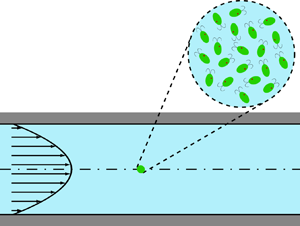
As depicted in figure 1, we consider a very dilute suspension of active particles in a 2-D channel flow. For instance, Chlamydomonas algae swimming in a quasi-2-D microfluidic channel or magnetic particles forced to swim in a plane by a strong magnetic field. If the volume fraction is low (e.g. concentration much less than  $1 \times 10^{6}\ \textrm {cells}\,\textrm {cm}^{-3}$ for algae with diameters less than
  $10\ \mathrm {\mu }\textrm {m}$), the cell–cell and cell–fluid interactions can be neglected (Bees Reference Bees2020). Particles are idealised as points. The transport equation in the position–orientation space (phase space) (Doi & Edwards Reference Doi and Edwards1988) can be adopted as
 $$\begin{gather} \frac{\partial P}{\partial t} + \left[ {Pe}_f u (y) + {Pe}_s \cos \theta \right] \frac{\partial P}{\partial x} + {Pe}_{\mathrm{s}} \sin \theta \frac{\partial P}{\partial y} + \frac{\partial}{\partial \theta} [\varOmega (y, \theta) P]\nonumber\\ = D_t \frac{\partial^2 P}{\partial x^2} + D_t \frac{\partial^2 P}{\partial y^2} + \frac{\partial^2 P}{\partial \theta^2}, \end{gather}$$
where  $t$ is the time,
  $x$ and
  $y$ are the position coordinates,
  $\theta$ is the angle between the swimming direction
  $\boldsymbol {p}$ of the particle and the longitudinal unit vector and
  $P(x,y,\theta ,t)$ is the p.d.f.

Figure 1. Sketch of a dilute suspension of active particles in a plane Poiseuille flow.
Following Jiang & Chen (Reference Jiang and Chen2019a), we have used the following dimensionless variables and parameters (the superscript  $\ast$ denotes dimensional variables) as
 \begin{equation} \left. \begin{aligned} t & = t^{{\ast}} D^{{\ast}}_r, \quad x = \frac{x^{{\ast}}}{W^{{\ast}}} - {Pe}_f t, \quad y = \frac{y^{{\ast}}}{W^{{\ast}}}, \quad u = \frac{u^{{\ast}}}{u^{{\ast}}_m} -1 ,\\ \varOmega & = \frac{\varOmega^{{\ast}}}{D^{{\ast}}_r},\quad {Pe}_s = \frac{V_s^{{\ast}}}{D^{{\ast}}_r W^{{\ast}}}, \quad {Pe}_f = \frac{u^{{\ast}}_m}{D^{{\ast}}_r W^{{\ast}}}, \quad D_t = \frac{D^{{\ast}}_t}{D^{{\ast}}_r (W^{{\ast}})^2}, \end{aligned} \right\} \end{equation}
where  $D^{\ast }_r$ is the rotational-diffusion coefficient,
  $W^{\ast }$ is the channel width,
  $u(y)$ is the velocity profile,
  $u^{\ast }_m$ is the mean flow speed
 \begin{equation} u^{{\ast}}_m \triangleq \frac{1}{W^{{\ast}}} \int^{W^{{\ast}}}_0 u^{{\ast}} (y^{{\ast}}) \, {\mathrm{d}} y^{{\ast}}, \end{equation}
 $\varOmega$ is the rate of change of
  $\theta$ (angular velocity),
  $V_s^{\ast }$ is the swimming speed of the active particle,
  ${Pe}_s$ is the corresponding swimming Péclet number,
  ${Pe}_f$ is the flow Péclet number and
  $D_t$ is the ratio of the translational diffusivity to the rotational diffusivity. We assume that the translational diffusivity is isotropic. Note that the dimensionless velocity profile is the deviation from the mean flow speed because we have transformed the frame of reference to that moving with the mean flow speed.
Due to the rotational and straining motion of the fluid, the rate of change of swimming direction for an ellipsoidal particle is given by Jeffery's equation (Jeffery Reference Jeffery1922; Leal & Hinch Reference Leal and Hinch1972; Pedley & Kessler Reference Pedley and Kessler1992; Lauga Reference Lauga2020) as
 \begin{equation} \varOmega (y, \theta) = \frac{{Pe}_f}{2} \frac{\mathrm{d} u}{\mathrm{d}y} [{-}1 + \alpha_0 \cos (2 \theta)], \end{equation}
where  $\alpha _0$ is the shape factor of the particle, with
  $\alpha _0 = 0$ for a spherical particle and
  $\alpha _0=1$ for an infinitely thin rod-like particle.
2.2. Boundary conditions and initial condition
For the solid boundaries, we consider two different types of condition. First, the reflective condition assumes that collisions between particles and solid boundaries are perfectly elastic (Bearon et al. Reference Bearon, Hazel and Thorn2011; Volpe et al. Reference Volpe, Gigan and Volpe2014; Jiang & Chen Reference Jiang and Chen2019a, Reference Jiang and Chen2020), Thus, it requires that both the incident swimming probability flux and the incident translational-diffusion probability flux through the walls are balanced by their corresponding reflective fluxes. Namely,
 \begin{equation} \left. \begin{aligned} P (x, y, \theta, t) & = P (x, y, - \theta, t), \quad \mathrm{at} \ y = 0, 1,\\ \frac{\partial P}{\partial y} (x, y, \theta, t) & ={-} \frac{\partial P}{\partial y} (x, y, - \theta, t), \quad \mathrm{at} \ y = 0, 1, \end{aligned} \right\} \end{equation}
ensuring the conservation of particles in the phase space.
Second, we consider the equally typical Robin condition (Enculescu & Stark Reference Enculescu and Stark2011; Ezhilan & Saintillan Reference Ezhilan and Saintillan2015; Jiang & Chen Reference Jiang and Chen2019a) to account for the wall accumulation phenomenon of some kinds of active particles, e.g. sperm cells and E. coli (Rothschild Reference Rothschild1963; Berke et al. Reference Berke, Turner, Berg and Lauga2008). For each swimming direction, there is no penetration of the probability flux through the walls. Namely,
 \begin{equation} D_t \frac{\partial P}{\partial y} = {Pe}_s \sin \theta P \quad \mathrm{at} \ y = 0, 1, \end{equation}
which is a third-type boundary condition. To balance the incident swimming flux, the wall-normal translational-diffusion flux must be negative, which leads to the accumulation of particles swimming towards a wall (Ezhilan & Saintillan Reference Ezhilan and Saintillan2015). Note that this mechanism for wall accumulation does not consider the complicated hydrodynamic and steric interactions between particles and walls (Lauga & Powers Reference Lauga and Powers2009; Bechinger et al. Reference Bechinger, Di Leonardo, Löwen, Reichhardt, Volpe and Volpe2016).
In the orientation space, periodic boundary conditions are imposed:
 \begin{equation} \left. \begin{aligned} P |_{\theta ={-}{\rm \pi}} & = P |_{\theta = {\rm \pi}},\\ \left. \frac{\partial P}{\partial \theta} \right|_{\theta ={-}{\rm \pi}} & = \left. \frac{\partial P}{\partial \theta} \right|_{\theta = {\rm \pi}} . \end{aligned} \right\} \end{equation}
 For the initial condition, we consider particles instantaneously released at a cross-section of the channel swimming in random directions with an arbitrary transverse concentration distribution  $C(y)$, i.e.
 \begin{equation} P |_{t = 0} = \frac{1}{2 {\rm \pi}} \delta(x) C(y), \end{equation}
where  $\delta$ is the Dirac delta function. There is no doubt that the initial condition will greatly impact the transient dispersion process of active particles but does not influence the long-time asymptotic behaviour.
3. Solutions of transient dispersion characteristics
The dispersion process of active particles in the longitudinal direction is of particular interest because the longitudinal scale is much larger than the transverse scale for a unidirectional confined flow. Taking the longitudinal coordinate variable  $x$ as the global space variable, and the confined section variables
  $y$ and
  $\theta$ as the local space variables, previous studies (Jiang & Chen Reference Jiang and Chen2019a, Reference Jiang and Chen2020) have applied the generalised Taylor dispersion theory (Brenner Reference Brenner1982; Brenner & Edwards Reference Brenner and Edwards1993) to analyse the long-time asymptotic values of dispersion characteristics, such as the local distribution, the drift and dispersivity.
In this work, we focus on the temporal evolution of these basic dispersion characteristics. We first introduce the definition of the moments of p.d.f. and their governing equations. Then, we use the biorthogonal expansion method (Strand et al. Reference Strand, Kim and Karrila1987; Brezinski Reference Brezinski1991) to solve the moments. The auxiliary eigenvalue problem for the moments is solved by the Galerkin method with confined-section–orientation function series constructed for the reflective boundary condition and the Robin condition (Jiang & Chen Reference Jiang and Chen2019a) respectively.
3.1. Definitions of moments and dispersion characteristics
The dispersion characteristics are derived from the moments of the probability distribution of particles. First, the moments of p.d.f. are conventionally defined as (Aris Reference Aris1956; Brenner & Edwards Reference Brenner and Edwards1993)
 \begin{equation} P_n (y, \theta, t) \triangleq \int^{\infty}_{- \infty} x^n P (x, y, \theta, t) \, \mathrm{d}\kern0.06em x, \quad n = 0, 1, \ldots, \end{equation}
which are also called the local moments. We assume the moments always exist on the basis of physical reasoning. Note that the zeroth-order moment,  $P_0$, is the marginal p.d.f. of
  $y$ and
  $\theta$, and thus can be viewed as the local distribution of active particles in the
  $y$–
$y$– $\theta$ plane of the phase space (Ezhilan & Saintillan Reference Ezhilan and Saintillan2015; Jiang & Chen Reference Jiang and Chen2019a).
Second, we introduce the global moments, i.e. the moments of the cross-sectional mean concentration distribution  $\bar {P}$,
 \begin{equation} M_n (t) \triangleq
\int^{\infty}_{- \infty} x^n \bar{P} \, \mathrm{d}\kern0.7pt x =
\overline{P_n(y,\theta, t)} \quad n = 0, 1, \ldots,
\end{equation}
\begin{equation} M_n (t) \triangleq
\int^{\infty}_{- \infty} x^n \bar{P} \, \mathrm{d}\kern0.7pt x =
\overline{P_n(y,\theta, t)} \quad n = 0, 1, \ldots,
\end{equation}
and
 \begin{equation} \bar{P}(x,t) \triangleq \int^1_0 \int^{\rm \pi}_{-{\rm \pi}} P (x, y, \theta, t) \, \mathrm{d} \theta\, \mathrm{d}y. \end{equation}
We use the bar to denote the integration over the  $y$–
$y$– $\theta$ cross-section. Due to the conservation of particles, we have
  $M_0=1$.
The basic dispersion characteristics, i.e. the drift  $U_d$ and dispersivity
  $D_T$, are related to the first- and second-order global moments,
 $$\begin{gather} U_d (t) \triangleq \frac{\mathrm{d} \mu_x}{\mathrm{d} t} = \frac{\mathrm{d} M_1}{\mathrm{d} t}, \end{gather}$$
 $$\begin{gather}D_T (t) \triangleq \frac{1}{2} \frac{\mathrm{d} \sigma^2}{\mathrm{d} t} = \frac{1}{2} \frac{\mathrm{d} M_2}{\mathrm{d} t} - M_1 \frac{\mathrm{d} M_1}{\mathrm{d} t}, \end{gather}$$
where  $\mu _x$ and
  $\sigma$ are the expected value (mean displacement) and the standard deviation (
 $\mathrm {MSD}$), respectively,
 \begin{equation} \mu_x \triangleq \frac{M_1}{M_0} = M_1, \quad \sigma^2 \triangleq \frac{M_2}{M_0} - \frac{M^2_1}{M^2_0} = M_2 - M_1^2 . \end{equation}
Their long-time asymptotic values correspond to the coefficients used in the famous Taylor dispersion model (Taylor Reference Taylor1953, Reference Taylor1954). To some extent, their temporal evolution can outline the longitudinal transport process in the transient stage before the Taylor dispersion regime (Gill & Sankarasubramanian Reference Gill and Sankarasubramanian1970; Chatwin Reference Chatwin1970; Latini & Bernoff Reference Latini and Bernoff2001; Wu & Chen Reference Wu and Chen2014; Yang et al. Reference Yang, Tan, Zeng, Wu, Wang and Jiang2020; Guan et al. Reference Guan, Zeng, Li, Guo, Wu and Wang2021).
Apart from the above basic dispersion characteristics, one can also introduce the skewness of the p.d.f., to capture the asymmetry of distribution, especially in the initial stage after particle release (Chatwin Reference Chatwin1970; Wang & Chen Reference Wang and Chen2017; Jiang & Chen Reference Jiang and Chen2019b). The skewness  $\gamma _1$ is defined by the third-order cumulant
  $\kappa _3$ of the distribution as
 \begin{equation} \gamma_1 \triangleq \frac{\kappa_3}{\sigma^3}, \quad \kappa_3 \triangleq \frac{M_3}{M_0} - 3 \frac{M_2 M_1}{M_0^2} + 2 \frac{M_1^3}{M_0^3} = M_3 -3 M_2 M_1 +2 M_1^3. \end{equation}
3.2. Solutions of moments: biorthogonal expansion
3.2.1. Governing equation of moments
To obtain the transient dispersion characteristics, we solve the moments first. According to the definition of moments (3.1) and the governing equation of the p.d.f. (2.1) (Aris Reference Aris1956), we have
 \begin{equation} \frac{\partial P_n}{\partial t} +\mathcal{L}P_n = n (n - 1) D_t P_{n - 2} + n \left[ {Pe}_{{f}} u (y) + {Pe}_{{s}} \cos \theta \right] P_{n - 1}, \quad n = 0, 1, \ldots, \end{equation}
where
 \begin{equation} \mathcal{L} ({\cdot}) \triangleq {Pe}_{{s}} \sin \theta \frac{\partial}{\partial y} ({\cdot}) + \frac{\partial}{\partial \theta} \left[ \varOmega (y, \theta) ({\cdot}) - \frac{\partial}{\partial \theta} ({\cdot}) \right] - D_t \frac{\partial^2}{\partial y^2} ({\cdot})\end{equation}
is an operator corresponding to the transport equation in the  $y$–
$y$– $\theta$ cross-section. Here,
  $P_{- 1} = P_{- 2} = 0$ are introduced to write the governing equation for all the moments in the same form.
The boundary conditions of  $P_n$ (
 $n = 0, 1, \ldots$) are in the same form as those of
  $P$. Namely, for the reflective condition (2.5),
 \begin{equation} \left. \begin{aligned} P_n (y, \theta, t) & = P_n (y, - \theta, t), \quad \mathrm{at}\ y = 0, 1,\\ \frac{\partial P_n}{\partial y} (y, \theta, t) & ={-} \frac{\partial P_n}{\partial y} (y, - \theta, t), \quad \mathrm{at} \ y = 0, 1. \end{aligned} \right\} \end{equation}
For the Robin condition (2.6),
 \begin{equation} D_t \frac{\partial P_n}{\partial y} = {Pe}_s \sin \theta P_n \quad \mathrm{at} \ y = 0, 1. \end{equation}
In the orientation space,
 \begin{equation} \left. \begin{aligned} P_n |_{\theta ={-}{\rm \pi}} & = P_n |_{\theta = {\rm \pi}},\\ \left. \frac{\partial P_n}{\partial \theta} \right|_{\theta ={-}{\rm \pi}} & = \left. \frac{\partial P_n}{\partial \theta} \right|_{\theta = {\rm \pi}} . \end{aligned} \right\} \end{equation}
The initial conditions according to (2.8) are
 $$\begin{gather} P_0 |_{t = 0} = \frac{1}{2 {\rm \pi}} C(y), \end{gather}$$
 $$\begin{gather}P_n |_{t = 0} = 0, \quad n = 1, 2, \ldots. \end{gather}$$
We can also obtain the governing equation for the global moments. Note that according to the integration by parts formula, we have
 \begin{equation} \overline{\mathcal{L}P_n} = 0, \quad n = 0, 1, \ldots, \end{equation}
under both the reflective condition (3.10) and the Robin condition (2.6). Therefore,
 \begin{equation} \frac{\mathrm{d} M_n}{\mathrm{d} t} = n (n - 1) D_t M_{n - 2} + n \overline{\left( {Pe}_f u + {Pe}_s \cos \theta \right) P_{n - 1}}, \quad n = 1,2 \ldots. \end{equation}
In particular,
 \begin{equation} U_d = \overline{\left( {Pe}_f u + {Pe}_s \cos \theta \right) P_0}, \end{equation}
namely, the local-distribution-weighted average of the longitudinal velocity component.
3.2.2. Biorthogonal expansion
Note that the form of moment equation (3.8) is similar to that of the case of passive particles. Previous studies used the method of separation of variables or the integral transform method (Barton Reference Barton1983; Jiang & Chen Reference Jiang and Chen2019b) to derive a series expansion for the solutions. An auxiliary Sturm–Liouville problem was solved first to obtain the function basis for the expansion.
However, for the present case of active particles, the local operator  $\mathcal {L}$ (3.9) associated with the boundary conditions can be non-self-adjoint and these two previous methods are not feasible. Instead, we use the biorthogonal expansion method (an extension of the integral transform method) (Strand et al. Reference Strand, Kim and Karrila1987; Brezinski Reference Brezinski1991; Nambiar et al. Reference Nambiar, Phanikanth, Nott and Subramanian2019) to obtain series expansions for the local moments and the Galerkin method to solve the associated eigenvalue problem.
First, the auxiliary eigenvalue problem for the moment equation (3.8) is
 \begin{equation} \mathcal{L} f_i = \lambda_i \,f_i, \end{equation}
where  $\lambda _i$ is the eigenvalue (
 $i=1,2,\ldots ,$) and
  $f_i$ is the associated eigenfunction satisfying all the boundary conditions of
  $P_n$. For
  $\lambda _1=0$,
  $f_1$ corresponds to the long-time asymptotic solution of
  $P_0$, which was discussed in our previous paper (Jiang & Chen Reference Jiang and Chen2019a).
It is difficult to find the explicit expression of the solution of the associated eigenfunction  $f_i$, due to the complexity of
  $\mathcal {L}$ (3.9). We use the Galerkin method to approximately solve
  $\lambda _i$ and
  $f_i$. Suppose we have found a basis with functions satisfying the required boundary conditions. Detailed expressions of the bases for the reflective condition and the Robin condition are later shown in § 3.2.3. Now, with such a basis, denoted by
  $\{e_i\}_{i=1}^{\infty }$, we can expand the eigenfunction
  $f_i$ as
 \begin{equation} f_i = \sum_{j = 1}^{\infty} \phi_{i j} e_j, \end{equation}
where  $\phi _{i j}$ is the coefficient of the expansion. For the local operator
  $\mathcal {L}$, we can also express the corresponding bilinear form
  $A(\cdot , \cdot )$ with the basis. The elements of the corresponding matrix (denoted by
  $\boldsymbol{\mathsf{A}}$) are
 \begin{equation} A_{i j} = A(e_i, e_j) = \langle e_i, \mathcal{L} e_j \rangle, \quad i=1,2,\ldots, \ j=1,2,\ldots, \end{equation}
where  $\langle \cdot , \cdot \rangle$ denotes the associated inner product, shown later in § 3.2.3 for different boundary conditions. In matrix form, the weak formulation of the auxiliary eigenvalue problem (3.18) can be written as
 \begin{equation} \boldsymbol{\mathsf{A}} \boldsymbol{\phi}_i= \lambda_i \boldsymbol{\phi}_i, \end{equation}
where  ${\boldsymbol {\phi }}_i =\begin {pmatrix} \phi _{i 1}, & \phi _{i 2}, & \cdots \end {pmatrix} ^{\mathrm {T}}$ is the vector of the coefficients of
  $f_i$. Truncating the series (3.19) to some degree gives a Galerkin solution for the eigenfunction
  $f_i$.
Note that  $\lambda _i$ is the eigenvalue of the matrix
  $\boldsymbol{\mathsf{A}}$ and
  ${\boldsymbol {\phi }}_i$ is the corresponding eigenvector. Therefore, solving the eigenvalue problem of
  $\boldsymbol{\mathsf{A}}$ can give asymptotic solutions of the eigenvalues and eigenfunctions of (3.18). In fact, the set of solutions
  $\{\,f_i\}_{i=1}^{\infty }$ can also form a basis for the function space satisfying the boundary conditions of the moments
  $P_n$.
With the eigenvalue  $\lambda _i$ and eigenfunction
  $f_i$ solved, one can easily follow the work of Barton (Reference Barton1983) and expand the local moments as
 \begin{equation} P_n (y, \theta, t) = \sum_{i = 1}^{\infty} p_{n i} (t) \mathrm{e}^{-\lambda_i t} f_i (y, \theta), \quad n=0,1,\ldots, \end{equation}
where  $p_{n i}$ is the expansion coefficients. Using the method of separation of variables (or the integral transform), Barton (Reference Barton1983) derived the general expressions for the expansion coefficients
  $p_{n i}$ (for
  $n$ up to three) with the elements of the bilinear form defined using the velocity profile and the initial condition. See § 3 in his paper.
However, for the present case, the local operator  $\mathcal {L}$ (3.9) associated with the boundary conditions can be non-self-adjoint due to the swimming (
 ${Pe}_s \cos \theta$) and the angular velocity of active particles. In fact, the matrix
  $\boldsymbol{\mathsf{A}}$ of the local operator can be non-symmetric, resulting in complex eigenvalues and eigenvectors. Thus the set of functions
  $\{\,f_i\}_{i=1}^{\infty }$ can be non-orthogonal, i.e. the inner product
  $\langle \, f_i, \,f_j\rangle \neq 0$ for
  $i \neq j$. The orthogonality relation fails when applying the integral transform method to obtain
  $p_{n i}$.
Instead of using the orthogonality relation, one can find another set of functions which bears a so-called biorthogonality relation with  $\{\,f_i\}_{i=1}^{\infty }$. According to the biorthogonal expansion method (Strand et al. Reference Strand, Kim and Karrila1987; Brezinski Reference Brezinski1991), these dual basis functions, denoted by
  $\{\,f^{\star }_i\}_{i=1}^{\infty }$ (a superscript
  $\star$ denotes the dual counterpart), are the eigenfunctions of the adjoint operator of
  $\mathcal {L}$ (denoted
  $\mathcal {L}^{\star }$). The eigenvalue of
  $f^{\star }_i$ corresponds to that of
  $f_i$, i.e.
  $\lambda _i$. Therefore, after normalisation, we have the biorthogonality relation
 \begin{equation} \langle \,f^{{\star}}_i, f_j\rangle = \delta_{i j}, \end{equation}
where  $\delta$ is the Kronecker delta.
We can also use the Galerkin method with the base  $\{e_i\}_{i=1}^{\infty }$ to solve
  $f^{\star }_i$. Let
  $\boldsymbol{\mathsf{A}}^{\star }$ denote the corresponding matrix of
  $\mathcal {L}^{\star }$. Note that
  $\boldsymbol{\mathsf{A}}^{\star }$ is the transpose of
  $\boldsymbol{\mathsf{A}}$. Then we have
 \begin{equation} \boldsymbol{\mathsf{A}}^{{\star}} {\boldsymbol{\phi}}_i^{{\star}} = \lambda_i {\boldsymbol{\phi}}_i^{{\star}}, \end{equation}
where  ${\boldsymbol {\phi }}_i^{\star }$ is the coefficient vector of the solution for
  $f_i^{\star }$. Performing the series expansion using the same basis as (3.19), we have
 \begin{equation} f^{{\star}}_i = \sum_{i = 1}^{\infty} \phi^{{\star}}_{i j} e_j \end{equation}
and  ${\boldsymbol {\phi }}_i^{\star } =\begin {pmatrix} \phi ^{\star }_{i 1}, & \phi ^{\star }_{i 2}, & \ldots \end {pmatrix}^{\mathrm {T}}$. Note that the eigenvalues of
  $\boldsymbol{\mathsf{A}}^{\star }$ are the same as those of
  $\boldsymbol{\mathsf{A}}$ (Strand et al. Reference Strand, Kim and Karrila1987). In fact,
  $\{\,f^{\star }_i\}_{i=1}^{\infty }$ also forms a basis.
With the biorthogonal family  $\{\,f_i\}_{i=1}^{\infty }$ and
  $\{\,f^{\star }_i\}_{i=1}^{\infty }$, one can continue to use the expressions obtained by Barton (Reference Barton1983) for the expansion coefficients of moments in (3.22), just by replacing the orthogonality relation with the biorthogonal one. Detailed expressions in current notation are presented in Appendix A.
Once we obtain the time-dependent solutions of the moments, the corresponding dispersion characteristics, i.e. the drift  $U_d$, dispersivity
  $D_T$ and skewness
  $\gamma _1$ can be calculated according to their definitions (3.4), (3.5) and (3.7a,b) without difficulties. The last problem is to find the basis functions
  $\{e_i\}_{i=1}^{\infty }$ satisfying the boundary conditions of moments.
3.2.3. Basis functions for different boundary conditions
First, we discuss the case with the reflective condition (3.10). A reflective basis can be constructed using the method of separation of variables for the Laplace operator for the transport equation of active particles in a tube (Jiang & Chen Reference Jiang and Chen2020). Similarly, for the 2-D channel, a much simpler reflective basis can also be found for the Laplace operator, which is self-adjoint with respect to the reflective condition. The basis  $\{e_i\}_{i=1}^{\infty }$ used in the Galerkin method for (3.19) can be comprised of
 \begin{gather}\left.\begin{gathered}
\frac{1}{\sqrt{2 {\rm \pi}}}, \quad \frac{1}{\sqrt{\rm \pi}} \cos (m \theta), \quad \frac{1}{\sqrt{\rm \pi}} \cos (n {\rm \pi}y),\\
\sqrt{\frac{2}{\rm \pi}} \cos (n {\rm \pi}y) \cos (m \theta), \quad \sqrt{\frac{2}{\rm \pi}} \sin (n {\rm \pi}y) \sin (m \theta),
\end{gathered} \right\}
\end{gather}
\begin{gather}\left.\begin{gathered}
\frac{1}{\sqrt{2 {\rm \pi}}}, \quad \frac{1}{\sqrt{\rm \pi}} \cos (m \theta), \quad \frac{1}{\sqrt{\rm \pi}} \cos (n {\rm \pi}y),\\
\sqrt{\frac{2}{\rm \pi}} \cos (n {\rm \pi}y) \cos (m \theta), \quad \sqrt{\frac{2}{\rm \pi}} \sin (n {\rm \pi}y) \sin (m \theta),
\end{gathered} \right\}
\end{gather}
where  $n=1,2,\ldots$ and
  $m=1,2,\ldots$ A detailed derivation can be found in appendix B of Wang et al. (Reference Wang, Jiang, Chen, Tao and Li2021). The corresponding inner product is just the
  $L^2$ inner product, i.e.
 \begin{equation} \langle \,f, g \rangle \triangleq \int^1_0 \int^{\rm \pi}_{- {\rm \pi}} f (y, \theta) g (y, \theta) \, \mathrm{d} \theta\,\mathrm{d} y, \end{equation}
where  $f$ and
  $g$ are functions that belong to the reflective basis.
Second, for the Robin condition (3.11), the construction of a basis  $\{e_i\}_{i=1}^{\infty }$ in much more complicated, due to the swimming term with the coefficient
  ${Pe}_s \sin \theta$. Following Jiang & Chen (Reference Jiang and Chen2019a), a decomposition form for the moments is applied before using the method of separation of variables
 \begin{equation} P_n (y, \theta) = P_a (y, \theta) G_n (y, \theta), \quad n = 0, 1, \ldots, \end{equation}
where
 \begin{equation} P_a (y, \theta) = \exp \left[ \frac{{Pe}_s}{D_t} \left( y - \frac{1}{2} \right) \sin \theta \right] \end{equation}
satisfies the Robin condition (3.11), and  $G_n (y, \theta )$ is a modified moment satisfying a governing equation similar to (3.8). A detailed discussion can be found in § 5 of Jiang & Chen (Reference Jiang and Chen2019a). Note that the solid boundary condition is then changed from the Robin condition (3.11) to a Neumann condition (the second-type boundary condition),
 \begin{equation} \left. \frac{\partial G_n}{\partial y} \right|_{y = 0, 1} = 0, \quad n = 0, 1, \ldots. \end{equation}
In the orientation space,  $G_n$ satisfies the same periodic condition as (3.12). Using the method of separation of variables of the Laplace operator for
  $G_n$, the basis for the Robin condition can be constructed as
 \begin{equation} \left. \begin{gathered}
\frac{P_a}{\sqrt{2 {\rm \pi}}},
\quad \frac{P_a}{\sqrt{\rm \pi}}\cos (m \theta),
\quad \frac{P_a}{\sqrt{\rm \pi}}\sin (m \theta),
\quad \frac{P_a}{\sqrt{\rm \pi}} \cos (n {\rm \pi}y), \quad
\\
\sqrt{\frac{2}{\rm \pi}} P_a \cos (n {\rm \pi}y) \cos (m \theta), \quad
\sqrt{\frac{2}{\rm \pi}} P_a \cos (n {\rm \pi}y) \sin (m \theta) .
\end{gathered} \right\}
\end{equation}
\begin{equation} \left. \begin{gathered}
\frac{P_a}{\sqrt{2 {\rm \pi}}},
\quad \frac{P_a}{\sqrt{\rm \pi}}\cos (m \theta),
\quad \frac{P_a}{\sqrt{\rm \pi}}\sin (m \theta),
\quad \frac{P_a}{\sqrt{\rm \pi}} \cos (n {\rm \pi}y), \quad
\\
\sqrt{\frac{2}{\rm \pi}} P_a \cos (n {\rm \pi}y) \cos (m \theta), \quad
\sqrt{\frac{2}{\rm \pi}} P_a \cos (n {\rm \pi}y) \sin (m \theta) .
\end{gathered} \right\}
\end{equation}
The corresponding inner product is defined with a weight function as
 \begin{equation} \langle \,f, g \rangle \triangleq \int^1_0 \int^{\rm \pi}_{- {\rm \pi}} \frac{1}{P_a^2 (y, \theta)^{}} \,f (y, \theta) g (y, \theta) \, \mathrm{d} \theta \,\mathrm{d} y, \end{equation}
where  $f$ and
  $g$ are functions that belong to the Robin basis.
3.2.4. Summary of solution procedure
A flowchart of the solution procedure is presented in figure 2. In the calculation of truncated  $\{\,f_i\}_{i=1}^{N}$ and
  $\{\,f^{\star }_i\}_{i=1}^{N}$ by the Galerkin method, we collect terms with
  $n\leqslant 20$ and
  $m\leqslant 10$ to solve the eigenvalue problem (3.21), for both the reflective basis (3.26a–d) and the Robin basis (3.31a–d). The total numbers of basis functions are
  $431$ and
  $441$ respectively. Note that for large
  ${Pe}_s$ under the Robin condition, more terms are needed to optimise the precision because of the highly concentrated boundary layer of swimmers (Ezhilan & Saintillan Reference Ezhilan and Saintillan2015). For large
  ${Pe}_f$, the strong alignment of elongated swimmers in the shear flow also requires more basis functions (Ezhilan & Saintillan Reference Ezhilan and Saintillan2015; Jiang & Chen Reference Jiang and Chen2019a). In fact, with extreme parameters, one should perform an asymptotic analysis before applying the Galerkin method.

Figure 2. Flowchart of the solution procedure.
For the biorthogonal expansion of moments (3.22), we truncate the series with an upper bound of summation  $N=40$ to reduce the truncation error of the series expansion in the initial stage of the transport process, especially for the case of a point-source release. The terms are sorted by the real part of the complex eigenvalue because higher-order terms decay much more rapidly. The result by the biorthogonal expansion is verified with the numerical result by Brownian dynamics simulation, as shown in Appendix B. We solve the first four moments. The related dispersion characteristics, i.e. the drift
  $U_d$ (3.4), dispersivity
  $D_T$ (3.5) and skewness
  $\gamma _1$ (3.7a,b), are obtained accordingly.
4. Results
To compare the transient dispersion process of active particles with that of passive ones, we consider the case of active particles dispersing in a common plane Poiseuille flow. The dimensionless velocity profile is  $u(y) = 6 y (1-y) -1$. Previous studies (Jiang & Chen Reference Jiang and Chen2019a; Wang et al. Reference Wang, Jiang, Chen, Tao and Li2021) already discussed the long-time asymptotic values of the local distribution, drift and dispersivity. Here, we analyse the temporal evolution of these characteristics, as well as the skewness. Our result corresponds to the previous result by Jiang & Chen (Reference Jiang and Chen2019a) in the long-time asymptotic stage. We focus on the influences of the swimming, shear flow, initial condition, boundary effect (wall accumulation) and particle shape on the transient dispersion process. In the following studied cases, we fix the translation diffusion coefficient
  $D_t={1}/{6}$ based on the data of previous studies (Ezhilan & Saintillan Reference Ezhilan and Saintillan2015; Nili et al. Reference Nili, Kheyri, Abazari, Fahimniya and Naji2017; Jiang & Chen Reference Jiang and Chen2019a). We mainly discuss spherical particles (
 $\alpha _0=0$) for simplicity, while the shear-induced alignment of ellipsoidal particles is considered in § 4.5. Additionally, a comparison with the numerical result by the Brownian dynamics simulation is presented in Appendix B.
4.1. Influence of swimming
To analyse the swimming effect on the transient dispersion process, we consider spherical particles with different swimming abilities. Namely, the swimming Péclet numbers  ${Pe}_s$ are different and
  ${Pe}_s=0$ corresponds to the case of passive particles. To highlight the influence of swimming, there is no background shear flow (with the flow Péclet number
  ${Pe}_f =0$) and only the reflective boundary condition (3.10) is considered. Particles are released instantaneously at the middle of the cross-section of the channel, thus
  $C(y)$ in the initial condition (2.8) is
  $\delta (y-0.5)$.
4.1.1. Local distribution: zeroth-order moment
As shown in figure 3, to depict the temporal evolution of the local distribution,  $P_0$ at 3 small sample times (
 $t\in \{0.1, 0.3, 0.5\}$) is plotted. As expected, the local transport process of active particles is greatly different from that of passive particles. Without swimming, passive particles perform pure translational Brownian motions, while the rotational diffusion of the ‘swimming’ direction takes no effect due to the uniform initial distribution of the swimming direction. As shown in figure 3(a–c), the distribution for
  $\theta$ is uniform, while in the transverse direction, the distribution become more and more uniform as particles spread out gradually;
  $P_0$ is symmetric with respect to the centreline of the channel due to the point-source release at
  $y=0.5$.

Figure 3. Density plot of transient local distributions  $P_0(y,\theta ,t)$ of spherical particles with different swimming abilities. The swimming Péclet number: (a–c)
  ${Pe}_s =0$; (d–f)
  ${Pe}_s =0.1$; (g–i)
  ${Pe}_s =0.5$; (j–l)
  ${Pe}_s =1$; (m–o)
  ${Pe}_s =2$. Sample times: (a,d,g,j,m)
  $t=0.1$; (b,e,h,k,n)
  $t=0.3$; (c,f,i,l,o)
  $t=0.5$. In all cases,
  ${Pe}_f=0$ and the reflective boundary condition is used. Particles are released at
  $y=0.5$.
For the active particles, the local transport process is a combination of the swimming motion and translational diffusion. As shown in figure 3(d–o), the swimming of particles leads to a sinusoidal variation of the distribution in the  $O y \theta$ plane. Here,
  $P_0$ is not symmetric with respect to the centreline, but with respect to the point
  $(y=0.5, \theta =0)$, also as a result of the point-source release in a uniform swimming direction distribution. After the release, most particles swim towards walls, resulting in a depletion of distribution in the middle of the channel during the transient transport process, as shown in figure 3(k,n) for particles with large swimming speeds. Meanwhile, the rotational diffusion of the swimming direction leads to the swimming-induced diffusion process and makes the distribution of
  $\theta$ uniform again. Moreover, in figure 3(m,n), the reflection of the swimming probability flux at the channel walls is observed, as a result of the elastic collisions described by the reflective boundary condition (2.5). Particles that swim towards the wall (e.g.
  $-{\rm \pi} <\theta <0$ at
  $y=0$) are reflected back to the bulk in the reversed direction (
 $-\theta$).
Both the local distributions of active and passive particles become uniform in the whole local space as time increases. Even when  $t=0.5$, as shown in figure 3(c,f,i,l,o), the distributions are very uniform. The results at larger times, not shown here, have nearly no difference between each other. In fact, in the long-time limit, the local distribution of spherical particles is exactly uniform (Jiang & Chen Reference Jiang and Chen2019a). Obviously, the distribution of particles with stronger swimming ability will reach the uniform equilibrium faster, due to the swimming-induced diffusion effect.
The swimming-induced diffusion effect on the local transport process can be demonstrated more clearly by the transverse distribution, defined as
 \begin{equation} C_t (y, t) \triangleq \int^{\rm \pi}_{- {\rm \pi}} P_0 (y, \theta, t) \, \mathrm{d} \theta . \end{equation}
As shown in figure 4, the larger  ${Pe}_s$, the smaller the concentration gradient. At
  $t=0.5$, shown in figure 4(c), the transverse distributions of cases with
  ${Pe}_s=1$ and
  $2$ are nearly uniform, while the distributions of cases with
  ${Pe}_s<1$ still have small fluctuations. As time continues to increase (not shown here), all the curves overlap each other and become absolutely uniform (Jiang & Chen Reference Jiang and Chen2019a). The transverse distribution of faster swimmers reaches the uniform equilibrium state much more quickly, as a result of the swimming-induced diffusion. For
  ${Pe}_s=2$, during the transport process, it is clearly observed that the initial high concentration distribution in the middle of the channel decreases fast, resulting in a depletion by the strong swimming effect, as shown in figure 4(b). The transport process in other cases is dominated by the comparable effects of the swimming-induced diffusion and translational diffusion.

Figure 4. Transverse distributions  $C_t(y,t)$ of spherical particles with different swimming abilities. Sample times: (a)
  $t=0.1$; (b)
  $t=0.3$; (c)
  $t=0.5$. In all cases,
  ${Pe}_f=0$ and the reflective boundary condition is used. Particles are released at
  $y=0.5$.
4.1.2. Dispersivity
Next, we discuss the transient dispersion characteristics related to the moments with order larger than zero. Note that we do not consider any background flow in this section. Therefore, the p.d.f. of particles is symmetric with respect to the  $y$-axis, where the particles are initially released. Both the drift and the skewness are zero because of this symmetry property. We only discuss the temporal evolution of the dispersivity.
As shown in figure 5, for active particles, the dispersivity increases monotonically with time. While for passive particles, the dispersivity remains the same as the translational-diffusion coefficient, because they only perform pure translational Brownian motions. In the initial stage of the dispersion process, the dispersivity of active particles, especially those with strong swimming ability (e.g.  ${Pe}_s=2$), is quite small. It then increases rapidly and finally reaches a stable value, i.e. the Taylor dispersivity. Obviously, the larger
  ${Pe}_s$, the larger the dispersivity. The difference between dispersivities with different
  ${Pe}_s$ is gradually enlarged during the transient dispersion process.

Figure 5. Temporal evolution of the dispersivity  $D_T(t)$ of spherical particles with different swimming abilities under the reflective condition without background flow (
 ${Pe}_f=0$). Particles are released at
  $y=0.5$.
Note that, without shear flow, the active dispersivity is only comprised of the swimming-induced diffusion (temporal) and the translational diffusion (time independent). Actually, in the longitudinal direction, the evolution of the active dispersivity is similar to that of the effective diffusion tensor (the time derivative of the mean squared displacement) in unbounded space (ten Hagen et al. Reference ten Hagen, van Teeffelen and Löwen2011a). There exists an anomalous dispersion stage before the Taylor dispersion regime (Wu et al. Reference Wu, Foufoula-Georgiou, Parker, Singh, Fu and Wang2019). Note that when  ${Pe}_s$ is large, the swimming-induced diffusion is the main factor of the dispersivity. In the initial stage (
 $t<0.5$) after the point-source release, the swimming of particles with rotational Brownian motions makes the local distribution uniform in the cross-section, as shown in figure 3(j,m,k,n). Namely, particles can swim randomly at different transverse positions. The swimming-induced dispersivity in the longitudinal direction is continuously enhanced, which leads to a super-diffusion process. The enhancement of dispersivity is stopped when the longitudinal length scale of the swimmer cloud is much larger than both the transverse length scale of the cross-section and the correlation length for a Brownian swimmer. The local distribution in the cross-section and the orientation space is nearly uniform at each longitudinal position, thus the dispersivity finally reaches its maximum value.
4.2. Influence of shear flow
We have discussed the swimming effect on the transient dispersion process. Now we focus on the influence of the shear flow and the combined effect of the shear-induced dispersivity and the swimming-induced diffusion. To compare with the cases without background flow in § 4.1, we analyse five cases with different  ${Pe}_f$ but a fixed
  ${Pe}_s=1$. In the same way, results of spherical particles at three small sample times are plotted to demonstrate the transient process, and only the reflective boundary condition (3.10) is considered. Particles are released instantaneously at
  $y=0.5$.
4.2.1. Local distribution: zeroth-order moment
In the initial stage soon after the point-source release, as shown in figure 6(a,d,g,j,m) with  $t=0.1$, the local distributions of swimmers in the plane Poiseuille flow with different
  ${Pe}_f$ are similar. The parallel flow carries the swimmers downstream quickly, but does not change their transverse positions. Therefore, the swimming diffusion effect is dominant in making the local distribution uniform. Note that the shear flow can rotate the swimming direction of the particle, which is similar to the rotational Brownian motion, and thus it can also weaken the swimming diffusion effect. However, in the middle of the channel, the vorticity of the flow is zero. Therefore, the vorticity-induced rotation is very weak until particles spread over the cross-section of the channel.

Figure 6. Density plot of transient local distributions  $P_0(y,\theta ,t)$ of spherical particles in flows with different flow rates. The flow Péclet number: (a–c)
  ${Pe}_f =0.1$; (d–f)
  ${Pe}_f =1$; (g–i)
  ${Pe}_f =2$; (j–l)
  ${Pe}_f =4$; (m–o)
  ${Pe}_f =5$. Sample times: (a,d,g,j,m)
  $t=0.1$; (b,e,h,k,n)
  $t=0.3$; (c,f,i,l,o)
  $t=0.5$. In all cases,
  ${Pe}_s=1$ and the reflective boundary condition is used. Particles are released at
  $y=0.5$.
As time increases, unlike the no-flow case discussed in § 4.1, swimmers in a plane Poiseuille flow will temporally accumulate at the point  $(y=0.5, \theta ={\rm \pi} )$ in the local space, as shown in figure 6(b,e,h,k,n) with
  $t=0.3$. Namely, particles mainly swim upstream and near the middle of the channel. This phenomenon can be explained using the dynamical systems theory. As discussed in previous studies (Zöttl & Stark Reference Zöttl and Stark2012, Reference Zöttl and Stark2013; Jiang & Chen Reference Jiang and Chen2019a), the transverse swimming velocity and the angular velocity can be viewed as a local velocity field in the local space. For the spherical particles in the plane Poiseuille flow,
  $(y=0.5, \theta ={\rm \pi} )$ is a centre (critical point), where particles perform the swing motion around the centreline of the channel (Zöttl & Stark Reference Zöttl and Stark2012) and closed orbits in the local space are formed. When the shear is strong, as shown in figure 6(k,n) with
  ${Pe}_f \in \{4,5\}$, this temporary accumulation is so intense that the local distribution forms a clear circular spot at
  $(y=0.5, \theta ={\rm \pi} )$ (also at
  $(y=0.5, \theta =-{\rm \pi} )$ due to the periodicity).
At larger times, the local distribution approaches the uniform distribution, the same as that without background flow discussed in § 4.1. This is also true for any case with a unidirectional flow. The long-time asymptotic local distribution of spherical swimmers under reflective boundary condition is a uniform distribution (Jiang & Chen Reference Jiang and Chen2019a). The critical point  $(y=0.5, \theta =-{\rm \pi} )$ is only a centre, not a stable node. Thus, the accumulation at
  $(y=0.5, \theta =-{\rm \pi} )$ dissipates gradually and the local distribution becomes more and more uniform, as shown in figure 6(c,f,i,l,o) with
  $t=0.5$. There is no doubt that, with stronger shear, the approach to the homogeneous equilibrium state will be much slower.
The approach to the uniform distribution in the local space can be demonstrated more clearly with the transverse distribution, defined in (4.1). Comparing figure 7(b) with the case without background flow in figure 4, there is no concentration depletion in the middle of the channel. Instead, the concentration at  $y=0.5$ is the highest, mainly due to the point-source release at the centreline of the channel. Note that the vorticity-induced centre-point accumulation in the transverse direction is not strong. The concentration of the active case with
  ${Pe}_f=5$ is higher than those with smaller
  ${Pe}_f$, but is lower than the passive case with the same
  ${Pe}_f$. When
  $t=0.5$ as shown in figure 7(c), the transverse distribution of swimmers in a low flow rate flow (small
  ${Pe}_f$) is nearly uniform. However, when
  ${Pe}_f$ is large enough, e.g.
  ${Pe}_f=4,5$, there are still observable variations of the transverse distribution from the uniform distribution. The attenuation of the accumulation is slow and the homogeneous equilibrium state will be reached at larger times (not shown here).

Figure 7. Transverse distributions  $C_t(y,t)$ of spherical particles in flows with different flow rates. Sample times: (a)
  $t=0.1$; (b)
  $t=0.3$; (c)
  $t=0.5$. ‘Passive’ denotes the case of passive particles (
 ${Pe}_s=0$). Other cases are of active particles with
  ${Pe}_s=1$. In all cases, the reflective boundary condition is used. Particles are released at
  $y=0.5$.
4.2.2. Drift
Next, we analyse the transient dispersion characteristics. First, we discuss the drift, i.e. the time derivative of the first-order mean concentration moment. Note that we have transformed the reference to that moving with the mean flow, as in (2.2). Thus, the drift discussed here is the average of the longitudinal component of the velocity of particles above the mean flow.
Unlike the case without background flow, the drift of swimmers in a plane Poiseuille flow is not zero in the transient stage, as shown in figure 8(a). In fact, the drift is not small and is positive when the flow rate (represented by  ${Pe}_f$) is large, especially in the initial stage soon after the point-source release in the middle of the channel, where the flow velocity is the largest in the cross-section and thus is larger than the mean flow rate. Then the drift decreases very fast as time increases, for both the active and passive cases. As shown in figure 8(a), all the curves fall to around zero before
  $t=0.5$. With a larger
  ${Pe}_f$, the initial drift is larger, and thus the decrease rate of the drift is faster.

Figure 8. Temporal evolution of dispersion characteristics of spherical particles in flows with different flow rates. (a) The drift  $U_d(t)$, (b) the dispersivity
  $D_T(t)$ and (c) the skewness
  $\gamma _1(t)$. ‘Passive’ denotes the case of passive particles (
 ${Pe}_s=0$). Other cases are of active particles with
  ${Pe}_s=1$. In all cases, the reflective boundary condition is used. Particles are released at
  $y=0.5$.
There are two main factors for the sharp drop of the drift: the advection and the swimming. First, the spread of particles from the highest-flow-velocity region (in the middle of the channel) to the low-flow-velocity region can reduce the advection velocity of the particles, for both the active and passive cases. Second, due to the swing motion of swimmers in the middle of the channel (centre-point accumulation as shown in figure 6k,n), particles mainly swim in the opposite direction to the flow (upstream  $\theta =\pm {\rm \pi}$). Thus, the corresponding contribution to the drift is negative. The drift of the active case with
  ${Pe}_f=5$ is smaller than that of the passive case. When the swimming effect is dominant (when
  ${Pe}_f$ is small), the overall drift can even be reduced to below zero, as shown by the curves with
  ${Pe}_f\in \{0.1, 1\}$ in figure 8(a). While the drift curves with larger
  ${Pe}_f$ (e.g.
  ${Pe}_f=4$) will remain positive during the whole transient stage.
After the sharp drop, the overall drift slightly increases with time, for all the curves of active particles in figure 8(a). Because the local distribution becomes more and more uniform as time increases, as shown in figure 6, the reduction of drift by the upstream swimming is weakened. At larger times ( $t>1$), all the drift curves approach zero. Because the long-time asymptotic local distribution is uniform, the corresponding overall drift by (3.16) is
 \begin{equation} \lim_{t \rightarrow \infty} U_d = \lim_{t \rightarrow \infty} \overline{\left( {Pe}_f u + {Pe}_s \cos \theta \right) P_0} = \overline{\left( {Pe}_f u + {Pe}_s \cos \theta \right)} = 0, \end{equation}
as discussed by our previous study (Jiang & Chen Reference Jiang and Chen2019a). The mass centre of the swimmer cloud finally moves with the mean flow rate. However, there are great differences among the approach-to-zero process of the drift with different  ${Pe}_f$. For small
  ${Pe}_f=1, 2$,
  $U_d$ increases to zero directly from the lowest negative value caused by the sharp drop. For larger
  ${Pe}_f=4, 5$,
  $U_d$ increases slowly for a while to some positive values, and finally decreases to zero. The curve with
  ${Pe}_f=4$ shows a fluctuation across the zero value, while the drift with
  ${Pe}_f=5$ remains positive, as a result of the complex combined reduction effect of the advection and the swimming.
4.2.3. Dispersivity
Next, we discuss the temporal evolution of dispersivity. In § 4.1.2, the dispersivity is only composed of the swimming-induced diffusion and the translational diffusion. Adding the effect of the shear flow makes the evolution of the dispersivity much more complicated. The overall dispersivity is not a simple superposition of the shear-enhanced dispersivity and the swimming-induced diffusion. In fact, the shear effect and the swimming effect can inhibit each other! To analyse the overall dispersivity, one should bear in mind the question of which effect is dominant.
When  ${Pe}_f$ is small, the swimming-induced diffusion is dominant in the dispersion process. As shown in figure 8(b), the curves with
  ${Pe}_f=0.1, 1, 2$ are similar to that without background flow in figure 5: the overall dispersivity increases monotonically with time. In the initial stage (
 $t<0.5$), the dispersivities with larger
  ${Pe}_f=1,2$ are larger and increase faster than that with
  ${Pe}_f=0.1$. Because the transverse distribution becomes more uniform due to the swimming, as shown in figure 7, the shear-enhanced dispersivity becomes stronger as the particles spread from the low shear-rate region (the middle of the channel) to the high shear-rate regions. The distribution of the swimming direction is still highly non-uniform, and thus the increase of the swimming-induced dispersivity is slow. However, at large times (
 $t>1$), the increases of the dispersivities with larger
  ${Pe}_f=1,2$ become smaller. More importantly, the long-time asymptotic values, i.e. the Taylor dispersivities, are much smaller than that with
  ${Pe}_f=0.1$ (Jiang & Chen Reference Jiang and Chen2019a). Note that, at large times, the swimming-induced diffusion gradually exerts its influence and regains the dominance in the dispersion process, as the whole local distribution becomes much more uniform. The shear-enhanced rotation of the swimming direction can weaken the swimming-induced diffusion, as discussed in § 4.2.1. Therefore, with larger
  ${Pe}_f=1,2$, the Taylor dispersivities dominated by the swimming-induced diffusion are smaller.
For large  ${Pe}_f$, as shown by the curves with
  ${Pe}_f=4, 5$ in figure 8(b), the evolution of the dispersivity is more complex and does not monotonically increase with time. Although
  ${Pe}_f$ is large, the swimming effect is still dominant in the initial stage (
 $t<0.5$) after the point-source release because the shear rate near the release position is low. The dispersivity of the active particles is larger than that of the passive ones, as shown by the curves with
  ${Pe}_f=5$. As the suspension cloud spreads across the cross-section of the channel, the shear-induced dispersivity becomes more and more important. There is a very rapid rise of the dispersivity in the initial transient stage, which is similar to the case with low
  ${Pe}_f$. It is followed by an obvious but small reduction of the dispersivity, as a result of the inhibition by the swimming-induced diffusion. Note that, in the case of passive particles, in the shear-dominant dispersion regime, increasing the translational diffusion will decrease the Taylor dispersivity (see (41) in the work of Aris Reference Aris1956). Similarly, the swimming-induced diffusion can also suppress the shear dispersion (Bearon et al. Reference Bearon, Hazel and Thorn2011; Jiang & Chen Reference Jiang and Chen2020). Finally, the dispersivity increases with time again and reaches the equilibrium state. For
  ${Pe}_f=4$, the long-time asymptotic value is smaller than the maximum value and that of the case without flow, as a result of the mutual inhibition of the shear dispersion and the swimming-induced diffusion. For
  ${Pe}_f=5$, the shear dispersion achieves absolute dominance: the finial value exceeds that without flow which is only composed of the swimming-induced diffusion and translational diffusion. However, it is still smaller than that of the passive particles as a result of the inhibition. See also § 4 in the work of Wang et al. (Reference Wang, Jiang, Chen, Tao and Li2021) and Appendix C.
4.2.4. Skewness
Finally, we discuss the skewness caused by the shear flow. As shown in figure 8(c), the temporal evolution of skewness is much more complicated than those of the drift and dispersivity. Similar to the case of passive particles (Aris Reference Aris1956; Aminian et al. Reference Aminian, Bernardi, Camassa, Harris and McLaughlin2016), the skewness is negative in the initial transient stage, as a result of the dominant advection effect by the plane Poiseuille flow. When  ${Pe}_f$ is small (e.g.
  ${Pe}_f=0.1, 1$), the swimming-induced diffusion effect is stronger than the advection effect. The skewness is small and negative in the initial stage, and then becomes positive as time increases. Note that the skewness under the pure swimming-induced diffusion is zero, as discussed in § 4.1.2. Thus, the positive skewness is due to the combined effect of the swimming-induced diffusion and the advection, more specifically, by the vorticity-induced rotation of the swimming directions of particles. For a plane Poiseuille flow, the vorticity-induced rotation is strong near the wall where the shear rate is large. Therefore, the cloud of particles in the middle of the channel travelling downstream disperses faster than that near the walls travelling upstream (relative to the mean flow rate), due to the swimming-induced diffusion. The downstream part of the mean distribution is more uniform in the longitudinal direction, which results in the positiveness of the skewness.
For the cases with large  ${Pe}_f$ (e.g.
  $\geqslant 2$), the advection effect is dominant. The negativeness of the skewness is obviously observed and the temporal variation of skewness is large at small times, which is similar to the passive case. The skewness first decreases as time increases (
 $0.1< t<0.5$), due to the advection effect. Then it greatly increases, because of the comprehensive combined effect of the swimming-induced diffusion and the advection.
Finally, at large times, the skewness gradually approaches zero, for all the cases in figure 8(c). This means that the asymmetry of the mean concentration distribution disappears and indicates that the distribution becomes Gaussian. The approach to zero (or to the Taylor dispersion regime) is very slow. Even when the dispersivity reaches its equilibrium value (approximately  $t>5$), there is still a small varying skewness of the mean concentration distribution.
4.3. Influence of initial condition
In the above discussion, the initial condition is a point-source release at  $y=0.5$ with
  $C(y)=\delta (y-0.5)$. To demonstrate the influence of the initial condition, here, we consider three additional initial conditions: a point-source release at
  $y=0.75$, a point-source release at
  $y=1$, and a line-source release with
  $C(y)=1$. Other parameters are fixed:
  ${Pe}_s=1$,
  ${Pe}_f =2$. The reflective boundary condition is used.
4.3.1. Local distribution: zeroth-order moment
Figure 9 demonstrates the transient local distributions of the cases with the point-source releases at  $y=0.75$ and
  $y=1$. There is no doubt that the initial condition can greatly affect the early stage of the transport process. Particles mainly stay in the lower half of the channel, which is strongly related to the release position. Due to the off-centre release,
  $P_0$ is no longer symmetric with respect to
  $(y=0.5, \theta =0)$ as in figure 6(g–i). After being released near the top wall
  $y=1$, particles that swim towards the top wall (
 $0<\theta <{\rm \pi}$) are soon reflected back, while particles that swim with direction
  $0<\theta <{\rm \pi}$ take more time to reach the bottom
  $y=0$. Therefore, the non-uniformity is larger than that of the centre-release case in figure 6(g–i).

Figure 9. Density plot of transient local distributions  $P_0(y,\theta ,t)$ of spherical particles with different initial conditions: (a–c)
  $C(y)=\delta (y-0.75)$; (d–f)
  $C(y)=\delta (y-1)$. Sample times: (a,d)
  $t=0.1$; (b,e)
  $t=0.3$; (c,f)
  $t=0.5$. In all cases,
  ${Pe}_s=1$,
  ${Pe}_f =2$, and the reflective boundary condition is used.
The non-uniformity of  $P_0$ can be demonstrated more clearly by the transverse distribution
  $C_t$, as shown in figure 10. We have added the curves of the centre-release case and the line-source case. Obviously, the peak of the transverse distribution is strongly affected by the released position, especially in figure 10(a). Note that
  $P_0$ of the line-source case is a constant in the local space under the reflective boundary condition (Jiang & Chen Reference Jiang and Chen2019a). Thus
  $P_0$ is also always in its equilibrium state although the dispersion process is still developing. Due to the off-centre release,
  $C_t$ of point-source cases released at
  $y=0.75$ and
  $y=1$ is no longer symmetric with respect to the centreline of the channel. As shown in figure 10(a),
  $C_t$ of the centre-release case is nearly uniform while those of the off-centre-release cases are still far from the equilibrium. As time increases, all of them will reach the same uniform state, ‘forgetting’ the information of the initial condition.

Figure 10. Transverse distributions  $C_t(y,t)$ of spherical particles with different initial conditions. Here,
  $y_0$ is the release position of a point source with
  $C(y)=\delta (y-y_0)$, while ‘Line source’ denotes the line-source release with
  $C(y)=1$. Sample times: (a)
  $t=0.1$; (b)
  $t=0.3$; (c)
  $t=0.5$. In all cases,
  ${Pe}_s=1$ and the reflective boundary condition is used.
4.3.2. Drift
Next, we discuss the dispersion characteristics with different initial conditions. As shown in figure 11(a), the initial condition can greatly affect the drift, especially in the very early stage of the transport process. First, for the line-source case, the drift is exactly zero, due to the time-independent uniform local distribution as discussed above. Second, for the point-source case, it is obvious that the drift is strongly related to the release position. The flow speed at the release position determines the initial value of the drift. Note that we have transformed the reference to that moving with the mean flow. Thus, in the early stage, the drift of the centre-release case ( $y_0=0.5$) is positive while that of the wall-release case (
 $y_0=1$) is negative. More notably, the temporal evolution curve of the drift of the wall-release case is nearly the inversion of the curve of the centre-release case. For the off-centre-release case with
  $y_0=0.75$, the drift is nearly zero during the whole dispersion process because of the small initial drift (flow speed relative to the mean
  $u(0.75)=0.125$). As time increases, the drift approaches zero for all the cases, as discussed by Jiang & Chen (Reference Jiang and Chen2019b).

Figure 11. Temporal evolution of dispersion characteristics of spherical particles with different initial conditions. (a) The drift  $U_d(t)$, (b) the dispersivity
  $D_T(t)$ and (c) the skewness
  $\gamma _1(t)$. Here,
  $y_0$ is the transverse position for a point-source release with
  $C(y)=\delta (y-y_0)$, while ‘Line source’ denotes the line-source release with
  $C(y)=1$. In all cases,
  ${Pe}_s=1$ and the reflective boundary condition is used.
4.3.3. Dispersivity
As shown in figure 11(b), the initial condition has a slight impact on the dispersivity, unlike the transverse distribution and the drift discussed above. Only small variations of  $D_T$ are observed in the early stage of the transport process. Note that the release position can affect the shear-enhanced diffusion and the swimming-induced diffusion (by the vorticity-induced rotation), but has no effect on the translational diffusion. In the very early stage, the translational diffusion and the swimming-induced diffusion are dominant. But with
  ${Pe}_s=1$, the swimming-induced diffusion is not strong. Therefore, the difference among the considered cases is small. The dispersivity of the line-source case is the largest because the shear-induced dispersivity is strong due to the non-uniformity of the velocity distribution over the whole cross-section. The shear rate at the centreline is zero, thus the dispersivity of the centre-release case is the smallest. Although the shear rate at the wall is the largest, the development of the dispersion process is strongly confined by the wall. So
  $D_T$ of the wall-release case is smaller than that of the case released at
  $y_0=0.75$. At large times,
  $D_T$ of all cases reaches the same equilibrium state. The transient time scales are nearly the same because the initial longitudinal length scales of these cases are infinitely small (instantaneously release with
  $\delta (x)$ in the initial condition (2.8)).
4.3.4. Skewness
Similar to the dispersivity, the skewness is slightly affected by the initial condition, as shown in figure 11(c). All of the considered cases have small values of skewness in the very early stage of the transport process, but the initial condition can change the sign of the skewness. Note that when  ${Pe}_f=2$, the advection effect is dominant, as discussed in § 4.2.4 for the shear flow. Therefore, the release position can affect the shear-induced asymmetry of the concentration distribution. For the off-centre-release case with
  $y_0=0.75$, the skewness is positive in the very early stage, while the skewness of the other three cases is negative. As time increases, the skewness will change its sign, as a result of the swimming-induced diffusion and the advection. The reason is similar to that discussed in § 4.2.4. At large times, the skewness of all the cases approaches zero.
4.4. Influence of boundaries: wall accumulation
The above-discussed cases are under the reflective boundary condition (3.10). Now we turn to the Robin condition (3.11) to consider the influence of wall accumulation on the transient dispersion process of spherical particles. To demonstrate the combined effect of wall accumulation with the shear flow and the swimming-induced diffusion, we choose six cases, with  ${Pe}_f\in \{0.1, 2, 5\}$ and
  ${Pe}_s\in \{0.1, 1\}$. The same three sample times are chosen to compare with the results without accumulation.
4.4.1. Local distribution: zeroth-order moment
As shown in figure 12, there are fundamental differences between the local distribution under the Robin condition and that in figure 6 under the reflective condition. At the very initial stage after the point-source release, the local distributions are similar under these two types of condition, mainly depending on the swimming ability ( ${Pe}_s$). As swimmers reach the wall, they gradually form an obvious and sustained accumulation among the incoming angle range (e.g.
  $-{\rm \pi} <\theta <0$ at the wall
  $y=0$). Under the Robin condition (3.11), there is no penetration of particles through the walls in the phase space, for each swimming angle. Therefore, particles can only change their swimming direction by rotational diffusion. The incoming swimming probability flux is balanced by the translational flux with a negative wall-normal concentration gradient, as clearly shown in figure 12(e,k) at
  $t=0.3$ with
  ${Pe}_s=1$. Meanwhile, for the outgoing swimming angle (
 $0<\theta <{\rm \pi}$), the value of the distribution is very small and a positive wall-normal concentration gradient is established at the walls. Taken together, particles mainly swim towards the walls and thus accumulate at the walls. At larger times, the local distribution with wall accumulation by the incoming flux of particles remains and does not become uniform as that under the reflective condition (Ezhilan & Saintillan Reference Ezhilan and Saintillan2015; Jiang & Chen Reference Jiang and Chen2019a). Namely, the equilibrium state of the local transport under the Robin condition is not homogeneous. The wall accumulation process can be demonstrated more clearly using the transverse distribution, as defined in (4.1) and shown in figure 13.

Figure 12. Density plot of transient local distributions  $P_0(y,\theta ,t)$ of spherical particles under the Robin condition. The Péclet numbers: (a–c)
  ${Pe}_s=0.1, {Pe}_f=0.1$; (d–f)
  ${Pe}_s=1, {Pe}_f=0.1$; (g–i)
  ${Pe}_s=0.1, {Pe}_f=2$; (j–l)
  ${Pe}_s=1, {Pe}_f=2$; (m–o)
  ${Pe}_s=0.1, {Pe}_f=5$; (p–r)
  ${Pe}_s=1, {Pe}_f=5$. Sample times: (a,d,g,j,m,p)
  $t=0.1$; (b,e,h,k,n,q)
  $t=0.3$; (c,f,i,l,o,r)
  $t=0.5$.

Figure 13. Transverse distributions  $C_t(y,t)$ of spherical particles under the Robin condition. Sample times: (a)
  $t=0.1$; (b)
  $t=0.3$; (c)
  $t=0.5$.
Comparing the local distribution with different  ${Pe}_s$ and
  ${Pe}_f$ in figures 12 and 13, the wall accumulation is enhanced by a stronger swimming ability but is suppressed by the shear flow. When
  ${Pe}_s=1$, the accumulation strength and the incoming-angle-preferred orientation distribution are completely distinct from those with
  ${Pe}_s=0.1$. The stronger the incoming swimming probability flux, the larger the wall-normal concentration gradient, and thus the stronger the wall accumulation. As for the influence of the shear flow, when
  ${Pe}_f$ is large enough and the vorticity-induced rotation is strong, as shown in figure 12(q,r) and figure 13(c), the wall accumulation is greatly weakened and even disappears. Additionally, the incoming-angle-preferred distribution of
  $\theta$ remains but is nearly confined to only the half of the range, e.g.
  $-{\rm \pi} <\theta <-{\rm \pi} /2$ at the wall
  $y=0$. As discussed in § 4.2.1 and previous studies (Zöttl & Stark Reference Zöttl and Stark2012; Jiang & Chen Reference Jiang and Chen2019a), the vorticity-induced swing motions of particles around the centreline of the channel lead to the centre-point accumulation in the local space, which compensates the centreline depletion by the Robin condition. Furthermore, particles mainly swim upstream (parallel to the streamline). Thus, the incoming flux is weakened, reducing the strength of the wall accumulation.
4.4.2. Drift
Next, we discuss the dispersion characteristics under the Robin condition. First, for the drift shown in figure 14(a), there is a sharp drop in the very initial stage, similar to the result shown in figure 8(a) under the reflective condition. The advection and the swimming are the two key factors for the drift drop, as discussed in § 4.2.2. For the current case, the accumulation is the third main contributor. Near the walls, the flow speed relative to the mean flow rate is negative. Thus, the growing accumulation of particles at the walls drives them to move upstream, which can greatly decrease the drift, the local-distribution-weighted average of the longitudinal component of velocity, as shown in (3.17). At large times, the wall-accumulation-reduced drift even becomes negative, which is fundamentally different from the case under the reflective boundary condition. The reason is that the equilibrium state of the local distribution under the Robin condition is not homogenous, as discussed in our previous study (Jiang & Chen Reference Jiang and Chen2019a).

Figure 14. Temporal evolution of dispersion characteristics of spherical particles under the Robin condition. (a) The drift  $U_d(t)$, (b) the dispersivity
  $D_T(t)$ and (c) the skewness
  $\gamma _1(t)$.
As shown in figure 14(a), the initial value of the drift is highly related to  ${Pe}_f$, which indicates that the advection effect is dominant for the drift in the very initial stage. The decrease of the drift can be non-monotonic, especially when both
  ${Pe}_f$ and
  ${Pe}_s$ are large. For example, the drift curves with
  ${Pe}_s=1, {Pe}_f=1$ and
  ${Pe}_s=1, {Pe}_f=5$ rise slightly after the rapid drop, which is similar to the case under the reflective boundary condition, as discussed in § 4.2.2. The long-time asymptotic mainly depends on
  ${Pe}_s$ because the swimming ability mainly determines the strength of the wall accumulation, as discussed in § 4.2.1. With small
  ${Pe}_s=0.1$, the wall accumulation is weak, thus the equilibrium drift is nearly zero for all the cases with different
  ${Pe}_f$. With
  ${Pe}_s=1$, the equilibrium drift is negative and far from zero due to the strong wall accumulation.
4.4.3. Dispersivity
Now we turn to the temporal evolution of the dispersivity. As shown in figure 14(b), there is an overall upward trend of the dispersivity, from a small initial value to the larger Taylor dispersivity, which is similar to the case under the reflective boundary condition discussed in § 4.2.3. In the very initial stage, the wall accumulation is not fully formed because most particles are still far away from the walls after the point-source release, as discussed in § 4.4.1. Therefore, the increase of the dispersivity is the combined result of the shear dispersion, swimming-induced diffusion and translational diffusion.
As particles spread toward the walls, the wall accumulation exerts its influence, especially for the cases with large values of both  ${Pe}_s$ and
  ${Pe}_f$. Comparing the curve with
  ${Pe}_s=1$ and
  ${Pe}_f=2$ in figure 14(b) with that in figure 8(b) under the reflective condition, the accumulation makes the dispersivity decrease earlier (around
  $t=0.5$) and more considerably. The dispersivity also experiences a slight rise after the drop, but finally approaches a smaller equilibrium value. As discussed in our previous study (Jiang & Chen Reference Jiang and Chen2019a), the wall accumulation can suppress the dispersion process in the plane Poiseuille flow, for both the swimming and advection effects. In the accumulation layer, particles mainly swim towards the wall, and thus the swimming-induced diffusion is weakened. On the other hand, particles accumulate near the low-flow-speed regions, and thus the advection effect by the relative velocity difference in the cloud of particles is also reduced. For the curve with
  ${Pe}_s=1$ and
  ${Pe}_f=5$, the combined effect of the shear dispersion and the wall accumulation is much more complex. The curve shows strong fluctuations in the transient stage (e.g.
  $0.3< t<1$). Note that the whole dispersion process is dominated by the advection effect. The strength of the wall accumulation is weakened, as discussed in § 4.4.1, thus the suppression of the dispersivity is very weak in the Taylor dispersion regime at large times.
It is of great interest to investigate whether the wall accumulation can slow down or accelerate the approach process to the Taylor dispersion regime, compared with the no-accumulation result under the reflective condition in § 4.2.3. To estimate the time scale before entering the Taylor dispersion regime, we introduce the relative percentage difference of dispersivity
 \begin{equation} r_D (t) \triangleq \frac{D_T (t) - D_T^{\infty}}{D_T^{\infty}} \times 100\,\%, \end{equation}
where  $D_T^{\infty } \triangleq \lim _{t \rightarrow \infty } D_T(t)$ is the Taylor dispersivity. A zero
  $r_D$ indicates that the Taylor regime is reached.
As shown in figure 15, comparing the results under the Robin condition and the reflective condition, the wall accumulation slightly influences the time scale for the Taylor regime. When  ${Pe}_f$ is small (e.g.
  ${Pe}_f=0.1$), the curves of
  $r_D$ are nearly the same and the Taylor regime is reached when
  $t\approx 5$, although the local distributions under these two boundary conditions are fundamentally different, as shown in figure 6(c) and figure 12(f). Note that, when the flow rate is small, the swimming-induced diffusion is dominant in the dispersion process. The difference between the Robin condition and the reflective condition is whether to change the direction of the transverse motion after a particle hits a wall, as discussed in Appendix B. However, the direction of the longitudinal motion remains unchanged under both conditions. Therefore, the overall longitudinal dispersion process is similar under these two conditions. When
  ${Pe}_f$ is larger (e.g.
  ${Pe}_f=2$), although the temporal variations of
  $r_D$ are quite different under these two boundary conditions, they approach zero nearly at the same time (
 $t<5$). Only when
  ${Pe}_f$ is very large (e.g.
  ${Pe}_f=5$), can the wall accumulation, to some extent, hinder the dispersion process: there is still a small fluctuation of dispersivity under the Robin condition when the dispersivity under the reflective condition is nearly steady.

Figure 15. Temporal evolution of the relative percentage difference  $r_D(t)$ of dispersivity for spherical particles under different boundary conditions. ‘Robin’ denotes the Robin condition, and ‘Reflective’ denotes the reflective condition. In all cases, the swimming Péclet number
  ${Pe}_s=1$.
4.4.4. Skewness
Finally, we discuss the temporal evolution of the skewness. Overall, the wall accumulation can enhance the skewness for both the dispersion regimes dominated by the swimming-induced diffusion and the advection. First, in the initial stage, the evolution of the skewness is similar to that under the reflective boundary condition. Comparing figure 14(c) with figure 8(c), the skewness is negative, due to the advection effect. It first decreases and then increases as time increases. When  ${Pe}_f$ is small, the swimming-induced diffusion effect is dominant in the dispersion process. The negative skewness rises and becomes positive at larger times, because of the strong vorticity-induced rotation of the swimming directions of particles near the walls, as discussed in § 4.2.4 for the reflective boundary condition. Therefore, under the Robin condition, the wall accumulation makes the positive skewness larger. Much more particles concentrate near the walls and disperse slower than those near the centreline of the channel. When
  ${Pe}_f$ is large and the advection effect is dominant in the dispersion process, the absolute value of the skewness under the Robin condition is larger than that under the reflective condition. This is because the shear-enhanced dispersivity is larger near the walls where the shear rate is larger for the plane Poiseuille flow. The wall accumulation can thus strengthen the advection effect. At large times, the skewness gradually approaches zero for all the cases, which is similar to that under the reflective condition, although the decay process under the Robin condition is slower.
4.5. Influence of particle shape: shear-induced alignment
The above discussion considers only the spherical particles. Now we focus on the general case of ellipsoidal particles. Unlike spherical particles, ellipsoidal particles (with shape factor  $\alpha _0 > 0$) experience not only the rotation induced by the vorticity of the fluid but also the alignment induced by the strain motion of the fluid (Ezhilan & Saintillan Reference Ezhilan and Saintillan2015), as shown by Jeffery's equation (2.4) for the angular velocity. For infinitely thin rod-like particles (with
  $\alpha _0=1$), the shear-induced alignment makes them swim parallel to the streamlines, also called streamwise alignment (rheotaxis) (Pedley & Kessler Reference Pedley and Kessler1992). The steady values of the local distribution, drift and dispersivity for the case of
  $\alpha _0=1$ have been discussed in our previous study (Jiang & Chen Reference Jiang and Chen2019a). To demonstrate the effect of shear-induced alignment on the transient state and compare it with the above-discussed cases, we choose four cases of ellipsoidal particles with
  $\alpha _0 \in \{0.5, 1\}$ under the Robin condition and reflective boundary condition. Other parameters are fixed:
  ${Pe}_s = 1$, and
  ${Pe}_f =2$. The current temporal result corresponds to our previous result (Jiang & Chen Reference Jiang and Chen2019a) in the long-time asymptotic limit.
4.5.1. Local distribution: zeroth-order moment
As shown in figure 16, the shear-induced alignment of ellipsoidal particles significantly affects the distribution of the swimming direction during the transient dispersion process. First, for the Robin condition, it has been shown in figure 12(j,k,l) for spherical particles that the vorticity-induced rotation confines the incoming-angle-preferred distribution to nearly only the half of the range: particles mainly swim upstream near the walls ( $\theta =\pm {\rm \pi}$). The strain-induced alignment further enhances the upstream-preferred angle distribution. Additionally, some ellipsoidal particles near the walls can swim downstream, which is not observed in the spherical case.

Figure 16. Density plot of transient local distributions  $P_0(y,\theta ,t)$ of ellipsoidal particles under the Robin and reflective conditions: (a–c)
  $\alpha _0=0.5$, Robin condition; (d–f)
  $\alpha _0=1$; Robin condition; (g–i)
  $\alpha _0=0.5$, Robin condition; (j–l)
  $\alpha _0=1$, reflective condition. Sample times: (a,d,g,j)
  $t=0.1$; (b,e,h,k)
  $t=0.3$; (c,f,i,l)
  $t=0.5$. In all cases,
  ${Pe}_s = 1$,
  ${Pe}_f=2$.
Second, for the reflective condition, the vorticity-induced tendency to upstream swimming of spherical particles in the middle of the channel after the release is weakened for ellipsoidal particles. Comparing figure 16(g–l) with figure 6(g–i), ellipsoidal particles near the walls mainly swim upstream, the same as those under the Robin condition. While in the middle of the channel, some particles swim downstream, due to the shear-induced alignment effect, which is different from the spherical particles.
The shear-induced alignment of ellipsoidal particles can significantly change the distribution of  $\theta$. However, it impacts slightly on the transverse concentration distribution. As shown in figure 17, there are only small differences between the transverse distributions with different shape factors under the same boundary condition. The curves mainly depend on the type of boundary condition for the considered cases with
  ${Pe}_f =2$. The cloud of particles has reached the near-wall region by swimming before the shear-induced alignment exerts its full influence.

Figure 17. Transverse distributions  $C_t(y,t)$ of ellipsoidal particles under the Robin and reflective conditions. Sample times: (a)
  $t=0.1$; (b)
  $t=0.3$; (c)
  $t=0.5$. In all cases,
  ${Pe}_s = 1$,
  ${Pe}_f=2$.
4.5.2. Drift
We now discuss the temporal evolution of the drift, dispersivity and the skewness for ellipsoidal particles. First, as shown in figure 18(a), the effect of the shear-induced alignment on the drift is not large. In the very initial stage after the point-source release in the middle of the channel, the drift is positive due to the advection effect. The evolution of the drift of ellipsoidal particles with different shape factors is nearly the same as that of spherical particles. At large times, under the reflective condition, the drift of ellipsoidal particles diminishes with time, similar to that of spherical particles. Because the transverse distribution is nearly uniform, as shown in figure 17, the advection results in a small drift. The swimming effect is nearly balanced between the preferred directions of the shear-induced alignment. However, under the Robin conditions, the drift curves deviate from each other at large times. As discussed in § 4.4.2, the wall accumulation leads to a negative drift for spherical particles in the plane Poiseuille flow. For ellipsoidal particles, the shear-induced alignment further enhances the upstream swimming near the walls. The stronger the rheotaxis (larger  $\alpha _0$), the smaller the drift.

Figure 18. Temporal evolution of dispersion characteristics of ellipsoidal particles under the Robin and reflective conditions. (a) The drift  $U_d(t)$, (b) the dispersivity
  $D_T(t)$ and (c) the skewness
  $\gamma _1(t)$. In all cases,
  ${Pe}_s = 1$,
  ${Pe}_f=2$.
4.5.3. Dispersivity
Next, for the dispersivity, as shown in figure 18(b), the shear-induced alignment can enhance the dispersion process of ellipsoidal particles, especially at large times, for both the reflective boundary condition and the Robin condition. First, for the reflective condition, the dispersivity increases monotonically with time, similar to the spherical case in § 4.2.3. The shear-induced alignment makes the swimming direction of ellipsoidal particles tilt to the streamlines. Thus the swimming-induced longitudinal dispersivity is larger. Note that, because the slight impact of the shear-induced alignment on the transverse concentration distribution, the advection-enhanced dispersivity is almost unaffected by the alignment. Second, for the Robin condition, the wall accumulation can suppress the dispersion process, as discussed in § 4.4.3 for spherical particles, thus resulting in a drop of the dispersivity as time increases. The swimming-induced longitudinal dispersivity of ellipsoidal particles is also enhanced by the alignment, compensating some of the decreases.
4.5.4. Skewness
Finally, we discuss the skewness. Similar to the drift, the shear-induced alignment of ellipsoidal particles has a slight impact on the temporal evolution of the skewness, as shown in figure 18(c). In the very initial stage, the skewness of ellipsoidal particles is negative due to the advection, the same as that of spherical particles. Under the reflective condition, the differences between the skewness curves are small, for the same reasons as for the drift: the advection effects with different  $\alpha _0$ are comparable in nearly uniform transverse distributions, and the swimming effects are nearly balanced between the preferred directions. Under the Robin condition, the reduction of the swimming-induced diffusion by the strong vorticity-induced rotation near the walls makes the skewness positive, similar to that of spherical particles discussed in § 4.4.4. The shear-induced alignment ellipsoidal particles can enhance the swimming-induced diffusion in both the near-wall region and the middle of the channel. The overall effect enlarges the skewness. Namely, the cloud of particles swimming downstream disperses faster.
5. Concluding remarks
For the transient dispersion process of active particles in confined flows, this work makes a semi-analytical attempt to investigate the temporal evolution of the dispersion characteristics, including the local distribution in the confined-section–orientation space, the drift, dispersivity and skewness. To solve the moments of the p.d.f., the classic integral transform method for passive transport problems is not applicable due to the self-propulsion effect. We introduce the biorthogonal expansion method to overcome this difficulty. The auxiliary eigenvalue problem in the local space is solved by the Galerkin method using function series constructed for the reflective boundary condition and the Robin condition for the wall accumulation phenomenon respectively.
The detailed study on spherical and ellipsoidal swimmers dispersing in a plane Poiseuille flow clearly demonstrates the influences of the swimming, shear flow, initial condition, wall accumulation and particle shape on the transient dispersion process. After the point-source release at the centreline of the channel without background flow, the local distribution of active particles in the confined-section–orientation space becomes uniform faster than that of passive particles, as a result of the swimming-induced diffusion. With background flow, in the middle of the channel, the vorticity-induced rotation drives spherical particles to swim upstream and to perform swing motions. There is no doubt that the release position can greatly affect the transverse concentration distribution. Under the Robin condition, the wall accumulation is gradually formed as particles spread toward the walls. If imposing strong shear flow, the accumulation will diminish and the incoming-angle-preferred distribution near the walls will tilt upstream. The shear-induced alignment of ellipsoidal particles further enhances the upstream-preferred angle distribution near walls but impacts slightly on the transverse concentration distribution.
For the basic dispersion characteristics, the temporal evolution is complicated under the influences of the swimming, advection, initial condition and wall accumulation. Without advection, the drift and the skewness are zero due to the symmetry. The temporal dispersivity is similar to that in unbounded space, with an anomalous transient stage by the swimming-induced diffusion. If imposing the plane Poiseuille flow, the advection will lead to a large positive drift and negative skewness in the very initial stage, which are also greatly affected by the initial condition. The skewness can become positive at large times if the dispersion process is dominated by the swimming-induced diffusion. For the overall dispersivity, it is not a simple superposition of the shear-enhanced dispersivity and the swimming-induced diffusion. The wall accumulation can hinder the dispersion process by reducing both the shear-enhanced dispersivity and the swimming-induced diffusion. However, the accumulation slightly influences the time scale for the Taylor regime. The shear-induced alignment of ellipsoidal particles can enlarge the dispersivity but impacts slightly on the drift and the skewness.
It is interesting to extend the current analysis to various situations. First, this work only considers particles restricted in a 2-D channel flow, e.g. Chlamydomonas algae swimming in a quasi-2-D microfluidic channel (Kantsler et al. Reference Kantsler, Dunkel, Polin and Goldstein2013; Contino et al. Reference Contino, Lushi, Tuval, Kantsler and Polin2015; Ostapenko et al. Reference Ostapenko, Schwarzendahl, Böddeker, Kreis, Cammann, Mazza and Bäumchen2018). The 2-D configuration is often a simplification of the 3-D case in reality, already capturing many aspects of the swimming dynamics (Zöttl & Stark Reference Zöttl and Stark2012, Reference Zöttl and Stark2013). Only the component of the swimming direction projected onto the plane is considered. The particles can be tracked more easily in such a restricted compartment. However, the transport process of swimmers in a 3-D channel is much more complex. Due to the development of 3-D tracking techniques, e.g. digital holographic microscopy (Su, Xue & Ozcan Reference Su, Xue and Ozcan2012; Bianchi, Saglimbeni & Di Leonardo Reference Bianchi, Saglimbeni and Di Leonardo2017) and multi-view microscope (Buchner et al. Reference Buchner, Muller, Mehmood and Tam2021), more and more experimental studies have analysed the 3-D trajectories. Swimmers, e.g. Heterosigma akashiwo (Bearon Reference Bearon2013), may undergo helical trajectories. Not only the polar angle between the swimming direction and the longitudinal direction but also the azimuthal angle should be considered the governing equation (2.1). Besides, we only consider the plane Poiseuille flow. For the quasi-2-D channel with a large ratio of width to depth (Hele-Shaw channel), the velocity distribution is more uniform (across the width of the channel) than the parabolic profile (Chen et al. Reference Chen, Zeng, Wu, Gao and Zhao2017). One can apply the analytical solution of the velocity profile in a 3-D channel (Shah & London Reference Shah and London1978). Much more effort is needed to analyse the dispersion characteristics of swimmers in a 3-D channel, which is desirable for future work.
Second, this work has only considered very dilute suspensions. Future studies on dense suspensions should include particle–particle and particle–fluid interactions. The temporal evolution of the local distribution plays a key role in the analyses of the rheological property (Takatori & Brady Reference Takatori and Brady2017; Saintillan Reference Saintillan2018; Nambiar et al. Reference Nambiar, Phanikanth, Nott and Subramanian2019; Morris Reference Morris2020), self-organisation phenomenon, (Vicsek & Zafeiris Reference Vicsek and Zafeiris2012; Lushi, Wioland & Goldstein Reference Lushi, Wioland and Goldstein2014; Lushi, Goldstein & Shelley Reference Lushi, Goldstein and Shelley2018) and hydrodynamic instabilities (Pedley & Kessler Reference Pedley and Kessler1992; Hwang & Pedley Reference Hwang and Pedley2014; Bees Reference Bees2020). Moreover, besides the self-propulsion effect, taxes of active particles, such as gravitaxis (for gravity), chemotaxis (for chemical gradients) and phototaxis (for light) (Pedley & Kessler Reference Pedley and Kessler1992; Bees & Croze Reference Bees and Croze2014; Goldstein Reference Goldstein2015), probably have a great impact on the transient dispersion process.
Additionally, this work only considers a simple type of active particles, whose swimming speed is fixed and the swimming direction undergoes a rotational-diffusion process. The dispersion process of particles with other swimming mechanisms, e.g. the run-and-tumble dynamics of E. coli, is of great interest (Berg Reference Berg1993; Elgeti & Gompper Reference Elgeti and Gompper2015; Vennamneni, Nambiar & Subramanian Reference Vennamneni, Nambiar and Subramanian2020). Nevertheless, the influence of particles’ swimming behaviour near boundaries is also a fundamental issue. This work only considers two simple types of boundary condition, the reflective condition and Robin condition, both of which have imposed ideal assumptions. For swimmers without an obvious wall accumulation phenomenon, e.g. some artificial particles, the reflective condition is preferred in the transport model, whose equilibrium concentration distribution is uniform. For the case with highly concentrated boundary layers, the Robin condition is often used (Enculescu & Stark Reference Enculescu and Stark2011; Elgeti & Gompper Reference Elgeti and Gompper2013; Ezhilan & Saintillan Reference Ezhilan and Saintillan2015), but it does not account for the hydrodynamic particle–wall interactions. In experiments, the observed behaviour at boundaries can be much more complicated (Bianchi et al. Reference Bianchi, Saglimbeni and Di Leonardo2017; Lushi, Kantsler & Goldstein Reference Lushi, Kantsler and Goldstein2017), e.g. particles sliding along the surface (Sipos et al. Reference Sipos, Nagy, Di Leonardo and Galajda2015), scattering off (Volpe et al. Reference Volpe, Buttinoni, Vogt, Kümmerer and Bechinger2011; Kantsler et al. Reference Kantsler, Dunkel, Polin and Goldstein2013; Contino et al. Reference Contino, Lushi, Tuval, Kantsler and Polin2015) and the steric repulsion effect (Dehkharghani et al. Reference Dehkharghani, Waisbord, Dunkel and Guasto2019; Makarchuk et al. Reference Makarchuk, Braz, Araújo, Ciric and Volpe2019). Further work can consider these complex particle–wall interactions and develop appropriate boundary conditions (Fu, Perthame & Tang Reference Fu, Perthame and Tang2021) for the continuum transport model.
Funding
This work is supported by the National Natural Science Foundation of China (grant nos 51879002 and 51579004). W.J. acknowledges the support of the Shuimu Tsinghua Scholar Program.
Declaration of interests
The authors report no conflict of interest.
Appendix A. Expressions of moments by biorthogonal expansion
With the eigenvalues  $\{ \lambda _i \}_{i=1}^{\infty }$, the biorthogonal family
  $\{\,f_i\}_{i=1}^{N}$ and
  $\{\,f^{\star }_i\}_{i=1}^{N}$ and the associated inner product
  $\langle \cdot , \cdot \rangle$, one can use the expressions obtained by Barton (Reference Barton1983) for the solution of the moment equation (3.22). Note that Barton (Reference Barton1983) wrote the solutions in a general form with undermined eigenvalues and eigenfunctions. Therefore, we just need to substitute the corresponding eigenvalues and eigenfunctions for a different boundary condition into their expressions, and replace the orthogonality relation with the biorthogonal one. For short, here we just give expressions for the first three moments in current notation.
The zero-order moment (Barton Reference Barton1983, (3.5b))
 \begin{equation} P_0 = \sum^{N}_{i = 1} a_i \mathrm{e}^{- \lambda_i t} {f}_i, \end{equation}
where the coefficient related to the initial condition
 \begin{equation} a_i = \langle \,f^{{\star}}_i(y,\theta), \frac{1}{2 {\rm \pi}} C(y) \rangle, \quad i =1,2, \ldots \end{equation}
The first-order moment (Barton Reference Barton1983, (3.13))
 \begin{equation} P_1 = \sum^{N}_{i=1} a_i B_{i, i} t \mathrm{e}^{- \lambda_i t}{f}_i + \sum^{N}_{\substack{i,j=1 \\ j \neq i}} \frac{a_j B_{i, j} (\mathrm{e}^{- \lambda_j t} - \mathrm{e}^{-\lambda_i t}) }{\lambda_i - \lambda_j}\,f_i , \end{equation}
where the coefficient related to the velocity profile
 \begin{equation} B_{i, j} = \langle \,f_i^{{\star}} (y, \theta), [{Pe}_f u(y) + {Pe}_s \cos \theta] \,f_j(y,\theta) \rangle, \quad i, j = 1, 2, \ldots \end{equation}
The second-order moment
 \begin{align} P_2 &= \sum^{N}_{i=1} a_i B_{i, i}^2 t^2 \mathrm{e}^{- \lambda_i t} {f}_i +\sum^{N}_{i=1} 2 a_i D_t t \mathrm{e}^{-\lambda_i t} f_i\nonumber\\ &\quad +\sum^{N}_{\substack{i,j,k=1\\ k\neq j\land k\neq i}} \frac{2 a_k B_{j, k} B_{i, j} (\mathrm{e}^{- \lambda_k t} - \mathrm{e}^{-\lambda_i t}) }{(\lambda_k - \lambda_i) (\lambda_k - \lambda_j) }{f}_i +\sum^{N}_{\substack{i,j=1 \\ i\neq j}} \frac{2 a_i B_{j, i} B_{i, j} t \mathrm{e}^{- \lambda_i t} }{\lambda_j -\lambda_i} {f}_i\nonumber\\ &\quad +\sum^{N}_{\substack{i,j,k=1 \\ k\neq j\land j\neq i}} \frac{2 a_k B_{j, k} B_{i, j} (\mathrm{e}^{- \lambda_j t} - \mathrm{e}^{-\lambda_i t}) }{(\lambda_k - \lambda_j) (\lambda_i - \lambda_j)}{f}_i +\sum^{N}_{\substack{i,k=1 \\ k\neq i}} \frac{2 a_k B_{i, k} B_{i, i} t \mathrm{e}^{- \lambda_i t} }{\lambda_k -\lambda_i} {f}_i\nonumber\\ &\quad +\sum^{N}_{\substack{i,j=1 \\ j\neq i}} \frac{2 a_j B_{j, j} B_{i, j} [\mathrm{e}^{- \lambda_i t} - \mathrm{e}^{-\lambda_j t} + (\lambda_i - \lambda_j) t \mathrm{e}^{- \lambda_jt}]}{(\lambda_j - \lambda_i)^2} {f}_i . \end{align}
Appendix B. Comparison with Brownian dynamics simulation
To verify the solution of the moments by the biorthogonal expansion method, we perform a Brownian dynamics simulation, which is widely used in numerical studies (Croze et al. Reference Croze, Sardina, Ahmed, Bees and Brandt2013; Chilukuri et al. Reference Chilukuri, Collins and Underhill2015; Apaza & Sandoval Reference Apaza and Sandoval2016; Guo, Jiang & Chen Reference Guo, Jiang and Chen2020; Wu et al. Reference Wu, Singh, Foufoula-Georgiou, Guala, Fu and Wang2021). Attention should be paid to the treatment of the reflective and Robin boundary conditions.
According to the dimensionless governing equation (2.1), the corresponding stochastic differential equations for the coordinates of a swimmer  $(x(t), y(t), \theta (t))$ are
 \begin{equation} \left. \begin{array}{l} \dfrac{\mathrm{d}\kern0.06em x}{\mathrm{d} t} = {Pe}_f u (y) + {Pe}_s \cos \theta + \sqrt{2 D_t} \dfrac{\mathrm{d} W_x}{\mathrm{d} t},\\ \dfrac{\mathrm{d}y}{\mathrm{d} t} = {Pe}_s \sin \theta + \sqrt{2 D_t} \dfrac{\mathrm{d} W_y}{\mathrm{d} t},\\ \dfrac{\mathrm{d} \theta}{\mathrm{d} t} = \varOmega (y, \theta) + \sqrt{2 D_r} \dfrac{\mathrm{d} W_{\theta}}{\mathrm{d} t}, \end{array}\right\} \end{equation}
where  $W_x(t)$,
  $W_y(t)$ and
  $W_{\theta }(t)$ are independent standard Brownian motions. We simply apply a forward Euler scheme with time step
  $\Delta t$ for discretisation. The
  $n$th step coordinates of the swimmer are denoted as
  $(x_n, y_n, \theta _n)$. For the typical reflective boundary condition (2.5), if the swimmer exceeds the boundaries, then
 \begin{equation} \left. \begin{array}{ll@{}} y_n \rightarrow 2 - y_n, \quad \theta_n \rightarrow - \theta_n, & \mathrm{for} \ y_n > 1,\\ y_n \rightarrow - y_n, \quad \theta_n \rightarrow - \theta_n, & \mathrm{for} \ y_n <0, \end{array} \right\} \end{equation}
where  $\rightarrow$ means assignment. This treatment is common in Brownian dynamics simulations (Volpe et al. Reference Volpe, Gigan and Volpe2014; Bechinger et al. Reference Bechinger, Di Leonardo, Löwen, Reichhardt, Volpe and Volpe2016). For the Robin condition to account for the wall accumulation of swimmers,
 \begin{equation} \left. \begin{array}{ll@{}} y_n \rightarrow 2 - y_n, \quad \theta_n \rightarrow \theta_n, & \mathrm{for} \ y_n > 1,\\ y_n \rightarrow - y_n, \quad \theta_n \rightarrow \theta_n, & \mathrm{for} \ y_n > 1. \end{array} \right\} \end{equation}
Note that the swimming direction is not reversed as for the reflective condition after the collision with a wall. In fact, the Robin condition, or the no-penetration condition for the probability flux, can be viewed as a ‘reflective’ condition for the boundaries in the phase space with  $\theta$ treated as an extra position coordinate. Another similar treatment puts swimmers that exceed a wall back exactly at the wall, which is called a potential-free algorithm (Heyes & Melrose Reference Heyes and Melrose1993; Duzgun & Selinger Reference Duzgun and Selinger2018; Peng & Brady Reference Peng and Brady2020).
In the simulation, we use a small time step  $\Delta t = 10^{-3}$ to capture the transient transport process. Swimmers are initially put at
  $y_0=0.5$ with
  $\theta _0$ uniformly distributed in the interval
  $[-{\rm \pi} , {\rm \pi})$.
  $10^{5}$ trajectories are simulated for each case. As shown in figure 19, the semi-analytical result of the MSD of spherical swimmers by the biorthogonal expansion is in agreement with the numerical result by the Brownian dynamics simulation under both types of boundary condition.

Figure 19. Comparisons between the temporal evolution of  $\mathrm {MSD}$ of spherical particles by the biorthogonal expansion and Brownian dynamics simulation under different boundary conditions. ‘Robin’ denotes the Robin condition, and ‘Reflective’ denotes the reflective condition. In all cases,
  ${Pe}_s=1$,
  ${Pe}_f=2$.
Appendix C. Taylor dispersivity of particles with different swimming abilities
Figure 20 shows the Taylor dispersivity of active particles with different  ${Pe}_s$. Note that
  ${Pe}_f=5$ is large, thus when
  ${Pe}_s$ is small, the shear-induced dispersivity by advection is dominant. The Taylor dispersivity of active particles decreases as
  ${Pe}_s$ increases from zero (the case of passive particles), because the shear effect and the swimming effect can inhibit each other. However, when
  ${Pe}_s$ is large, the swimming-induced diffusion is dominant. Thus, the Taylor dispersivity increases with
  ${Pe}_s$.

Figure 20. Taylor dispersivity of spherical particles with different swimming abilities in a plane Poiseuille flow. For passive particles,  ${Pe}_s=0$. In all cases, the reflective boundary condition is used and
  ${Pe}_f=5$.


