2. Governing equations and numerical method

In present simulations we consider the non-reactive mono-species gases and Newtonian fluids for which the dynamic viscosity depends only on temperature. The governing equations for compressible turbulence in vibrational non-equilibrium can be written in the dimensionless form as

(2.1)$$\begin{gather} \frac{\partial {\rho}}{\partial {t}} + \frac{\partial(\rho u_j)}{\partial x_j} = 0, \end{gather}$$

(2.2)$$\begin{gather}\frac{\partial{(\rho u_i)}}{\partial {t}} + \frac{\partial{[\rho u_i u_j + p\delta_{ij}]}}{\partial{x_j}} = \frac{1}{Re} \frac{\partial{\sigma_{ij}}}{\partial{x_j}} + \mathcal{F}_i, \end{gather}$$

(2.3)$$\begin{gather}\frac{\partial{\varepsilon}}{\partial{t}} + \frac{\partial{[(\varepsilon + p)u_j]}}{\partial{x_j}}= \frac{1}{\alpha} \frac{\partial}{\partial{x_j}}\left(\kappa_{tr} \frac{\partial{T_{tr}}}{\partial{x_j}} + \kappa_v \frac{\partial{T_v}}{\partial{x_j}} \right) + \frac{1}{Re}\frac{\partial{(\sigma_{ij}u_i)}}{\partial{x_j}} - \varLambda + \mathcal{F}_I + \mathcal{F}_ju_j, \end{gather}$$

(2.4)$$\begin{gather}\frac{\partial{E_v}}{\partial{t}} + \frac{\partial{(E_vu_j)}}{\partial{x_j}} = \frac{1}{\alpha} \frac{\partial}{\partial{x_j}}\left(\kappa_v \frac{\partial{T_v}}{\partial{x_j}}\right) + \frac{E_v^*-E_v}{\tau_v}, \end{gather}$$

(2.5)$$\begin{gather}p = \rho T_{tr}/(\gamma_r M^2), \end{gather}$$

where the dimensionless density, velocity components, pressure, translational–rotational and vibrational temperatures are respectively denoted as $\rho$, $u_i$, $p$, $T_{tr}$ and $T_v$. The $\mathcal {F}_i$ and $\mathcal {F}_I$ are the large-scale forcings to the fluid momentum and translational–rotational energy, respectively. The velocity field is decomposed into a solenoidal component and a dilatational component. The large-scale forcing to the solenoidal velocity component is employed to maintain the velocity fluctuation within the two lowest wavenumber shells at prescribed levels, while the dilatational velocity component is left untouched. The large-scale forcing to the translational–rotational temperature is similar, while the prescribed levels are one percent of that for the solenoidal velocity component. The detailed forcing strategy has been given in Appendix A. Furthermore, the uniform thermal cooling function $\varLambda$ is adopted to sustain the internal energy in a statistically steady state (Passot, Vázquez-Semadeni & Pouquet Reference Passot, Vázquez-Semadeni and Pouquet1995; Wang et al. Reference Wang, Wang, Xiao, Shi and Chen2010). The $T_{tr}$ is employed in the equation of state (2.5), because the pressure mainly stems from the translational motion of molecules (Vincenti & Kruger Reference Vincenti and Kruger1965). The reference Reynolds number $Re \equiv \rho _r U_r L_r/\mu _r$, the reference Mach number $M \equiv U_r/c_r$ and the reference Prandtl number $Pr \equiv \mu _r C_{p_r}/\kappa _r$ are three governing parameters. Here, $\rho _r$, $U_r$, $L_r$ and $\mu _r$ are the reference density, velocity, length and viscosity coefficients, respectively. The reference speed of sound is given by $c_r = \sqrt {\gamma _r R T_r}$, where $R$ is the specific gas constant and $T_r = 1200K$ is the reference temperature. The $\gamma _r \equiv C_{p_r}/C_{v_r}$ is the ratio of specific heat at constant pressure $C_{p_r}$ to that at constant volume $C_{v_r}$. The $\gamma _r$ approximately equals 1.324 based on the specific heat ratio of dry air at $T_r = 1200$ K (Vincenti & Kruger Reference Vincenti and Kruger1965; Anderson Reference Anderson2006). The dimensionless parameter $\alpha$ is given as $\alpha \equiv PrRe(\gamma _r-1)M^2$, where $Pr$ is set to be 0.71.

The total energy per unit volume ($\varepsilon$), the vibrational energy per unit volume in thermal equilibrium ($E_v^*$) and non-equilibrium ($E_v$), and the viscosity stress ($\sigma _{ij}$) are respectively given as

(2.6)$$\begin{gather} \varepsilon = \rho \left(e_{tr} + e_v + \frac{1}{2} u_ju_j\right) = \frac{5}{2}p +E_{v} + \frac{1}{2}\rho (u_ju_j), \end{gather}$$

(2.7)$$\begin{gather}E_{v}^* = \rho e_{v}^* = \frac{\rho \theta_{v}}{\gamma_r M^2 [\exp(\theta_{v}/T_{tr}) -1]}, \end{gather}$$

(2.8)$$\begin{gather}E_{v} = \rho e_{v} = \frac{\rho \theta_{v}}{\gamma_r M^2 [\exp(\theta_{v}/T_v) -1]}, \end{gather}$$

(2.9)$$\begin{gather}\sigma_{ij} = \mu \left(\frac{\partial{u_i}}{\partial{x_j}} + \frac{\partial{u_j}}{\partial{x_i}}\right) - \frac{2}{3}\mu\theta\delta_{ij}, \end{gather}$$

where $e_{tr}$ is the translational–rotational energy per unit mass, while $e_v^*$ and $e_v$ are the vibrational energy per unit mass in thermal equilibrium and non-equilibrium, respectively. The $\theta _v$ is the characteristic vibrational temperature normalized by $T_r$, while $\theta = \partial u_k/\partial x_k$ is the velocity divergence. The temperature-dependent viscosity ($\mu$) and thermal conductivity coefficients ($\kappa _{tr}$ and $\kappa _{v}$) are specified by Sutherland's and Eucken's laws. For their detailed expressions, please refer to our previous publication (Zheng et al. Reference Zheng, Wang, Noack, Li, Wan and Chen2020).

In vibrational energy governing equation (2.4), the widely used Landau–Teller relaxation model is adopted for the vibrational rate $Q_v = (E_v^*-E_v)/\tau _v$. The dimensionless local relaxation time ($\tau _v$) depends closely on the local temperature and pressure, and is calculated roughly by (Vincenti & Kruger Reference Vincenti and Kruger1965)

(2.10)\begin{equation} \tau_v = (C/p)\textrm{exp}(K_2/T_{tr})^{1/3}, \end{equation}

where $C$ and $K_2$ are the dimensionless constants relating to the molecular structure of gases. Following the previous literature (Donzis & Maqui Reference Donzis and Maqui2016; Khurshid & Donzis Reference Khurshid and Donzis2019; Zheng et al. Reference Zheng, Wang, Noack, Li, Wan and Chen2020), the dimensionless parameter $\langle K_\tau \rangle = \langle \tau _v \rangle /\tau _\eta$ is adopted to characterize the time scale of the relaxation process. The $\langle \cdot \rangle$ operator stands for spatial average. The $\tau _\eta = [\langle \mu /(Re\rho )\rangle /\epsilon ]^{1/2}$ is the Kolmogorov time scale, $\epsilon =\langle \sigma _{ij}S_{ij}/Re \rangle / \langle \rho \rangle$ is the kinetic energy dissipation rate per unit mass due to viscosity and $S_{ij}=(\partial u_i/\partial x_j+\partial u_j/\partial x_i)/2$ is the strain rate tensor. The $K_2$ is set to be 2000.0, close to that in real gases. For instance, $K_2$ is respectively about 2460 and 1590 for oxygen and nitrogen molecules (Vincenti & Kruger Reference Vincenti and Kruger1965). Moreover, the constant $C$ is adjusted to obtain a specific $\langle K_\tau \rangle$ value.

The governing equations of compressible turbulence are solved in conservative form in a cubic box with the side length equaling $2{\rm \pi}$ and a $512^3$ grid resolution. The periodic boundary conditions in all three spatial directions are employed. The hybrid compact-weighted essentially non-oscillatory (compact-WENO) scheme is applied in present simulations. The hybrid scheme combines the eighth-order central compact finite difference scheme in smooth regions and the seventh-order WENO scheme in shock regions. The time derivative is approximated by the standard Runge–Kutta method. For more details of the numerical method, please refer to Lele (Reference Lele1992), Gottlieb & Shu (Reference Gottlieb and Shu1998), Balsara & Shu (Reference Balsara and Shu2000) and Wang et al. (Reference Wang, Wang, Xiao, Shi and Chen2010). After the system reaches the statistically stationary state, sixty-one flow fields, spanning the time period of $9.01 \lesssim t/T_e \lesssim 14.41$, are employed to obtain the statistical averages of interested quantities. Here, $T_e (= \sqrt {3}L_f/u^\prime )$ is the large eddy turnover time and $L_f$ is the integral length scale.

3. One-point statistics of compressible turbulence

The overall statistics of present simulations are summarized in tables 1–4. The reference Reynolds number and Prandtl number are kept constant ($Re = 400$ and $Pr = 0.71$). The reference Mach number ($M$) is set to be 0.099 and 0.296. For each Mach number, we control the characteristic vibrational temperature ($\theta _v$) and relaxation time ($\tau _v$) to investigate the vibrational non-equilibrium effect. In present simulations, three different $\theta _v$ ($\theta _v = 1.0$, 3.0 and 5.0) are employed. A lower $\theta _v$ suggests an easier excitation of the vibrational mode. Meanwhile, the $\tau _v$ is normalized as $\langle K_\tau \rangle$. The $\langle K_\tau \rangle$ approximately equals 0.16–9.80 for the $M = 0.099$ cases, and 0.19–7.98 for the $M = 0.296$ cases. Here, cases $\textrm {I}_1\text {--}\textrm {I}_4$ and cases $\textrm {II}_1\text {--}\textrm {II}_4$ (tables 1 and 3) are used to discuss the effect of $\langle K_\tau \rangle$, while cases $\textrm {I}_2, \textrm {I}_5$, $\textrm {I}_6$ and cases $\textrm {II}_2, \textrm {II}_5$, $\textrm {II}_6$ (tables 2 and 4) are adopted to study the effect of $\theta _v$.

Table 1. Simulation parameters and resulting flow statistics for the weakly compressible turbulence. Considering $\langle K_\tau \rangle$ effects. Here $M_t \approx 0.22$.

Table 2. Simulation parameters and resulting flow statistics for the weakly compressible turbulence. Considering $\theta _v$ effects. Here $M_t \approx 0.22$.

Table 3. Simulation parameters and resulting flow statistics for the highly compressible turbulence. Considering $\langle K_\tau \rangle$ effects. Here $M_t \approx 0.68$.

Table 4. Simulation parameters and resulting flow statistics for the highly compressible turbulence. Considering $\theta _v$ effects. Here $M_t \approx 0.68$.

The Taylor microscale Reynolds number ($Re_\lambda$) and turbulent Mach number ($M_t$) are respectively defined as

(3.1a,b)\begin{equation} Re_\lambda = Re\frac{\langle \rho \rangle u^\prime \lambda}{\sqrt{3}\langle \mu \rangle} \quad \textrm{and} \quad M_t = M\frac{u^\prime}{\langle \sqrt{T_{tr}} \rangle}, \end{equation}

where the root mean square (r.m.s.) value of velocity magnitude and the Taylor microscale are respectively given by

(3.2)$$\begin{gather} u^\prime = \sqrt{\langle u_1^2 + u_2^2 + u_3^2 \rangle} \end{gather}$$

(3.3)$$\begin{gather}\textrm{and} \quad \lambda = \sqrt {\frac{\langle u_1^2 + u_2^2 + u_3^2 \rangle}{\langle (\partial{u_1}/\partial{x_1})^2 + (\partial{u_2}/\partial{x_2})^2 + (\partial{u_3}/\partial{x_3})^2 \rangle}}. \end{gather}$$

Here, the $M_t$ approximately equals $0.22$ and $0.68$ for $M = 0.099$ and $0.296$ cases, respectively. The $Re_\lambda$ is considered to be constant for all cases. The $Re_\lambda \approx 157.5$, with the largest deviation at 2.0 % (tables 1–4).

The resolution parameter $\eta /{\rm \Delta} x$ is in the range of $1.01 \lesssim \eta / {\rm \Delta} x \lesssim 1.06$, where ${\rm \Delta} x$ is the grid length in each direction (tables 1–4). The resolution parameter $k_{max}\eta$ is therefore in $3.17 \lesssim k_{max}\eta \lesssim 3.33$, where the largest wavenumber $k_{max}$ is half of the number of grids $N$ in each direction (i.e. $k_{max} = N/2$). According to the previous grid refinement studies (Wang et al. Reference Wang, Shi, Wang, Xiao, He and Chen2011), the grid resolutions $k_{max}\eta \geq 2.77$ are enough for the convergence of flow statistics, including energy spectra at different wavenumbers, probability density functions (PDFs) of normalized dilatation and vorticity, etc.

The integral length scale is calculated by

(3.4)\begin{equation} L_f = \frac{3{\rm \pi}}{2(u^\prime)^2}\int^\infty_0 \frac{E^u(k)}{k}\textrm{d} k, \end{equation}

where $E^u(k)$ is the spectrum of kinetic energy per unit mass. The ratios $L_f/\eta$ and $T_e/\tau _\eta$ respectively represent the spatial and time scales in the simulated flows. The $\eta = [\langle \mu /(Re\rho )\rangle ^3/\epsilon ]^{1/4}$ is the Kolmogorov length scale. Presently, $L_f/\eta \approx 113.8$ and $T_e/\tau _\eta \approx 17.9$ (tables 1–4). The kinetic energy dissipation rate due to viscosity $(\epsilon )$ is about 0.70 for both the $M_t \approx 0.22$ and $0.68$ cases.

The vibrational rate represents the energy exchange rate between the translational– rotational and vibrational modes. Its r.m.s. value ($Q_{v,rms}$) can be employed to assess the strength of energy exchange. However, the proportion of vibrational mode in the internal energy should also be taken into account. The spatially averaged ratio of the vibrational energy to the total internal energy (i.e. $\langle E_v^*/[(5/2)p+E_v^*] \rangle$) approximately equals 18.88 %, 5.92 % and 1.34 % with $\theta _v = 1.0$, 3.0 and 5.0, respectively. Here, the parameter $\mathcal {H} (= \langle E_v^*/[(5/2)p+E_v^*] \rangle Q_{v,rms})$ is adopted, combining effects of $\theta _v$ and $\langle K_\tau \rangle$. For the $M_t \approx 0.22$ cases, $\mathcal {H}$ decreases from 3.39 to 1.24 as $\langle K_\tau \rangle$ increases from $0.16$ to $9.80$ (cases $\textrm {I}_1\text {--}\textrm {I}_4$, table 1), and decreases from 1.70 to 0.08 with $\theta _v$ varying from $1.0$ to $5.0$ (cases $\textrm {I}_2$, $\textrm {I}_5$ and $\textrm {I}_6$, table 2). For the $M_t \approx 0.68$ cases, $\mathcal {H}$ decreases from 1.07 to 0.22 as $\langle K_\tau \rangle$ increases from $0.19$ to $7.98$ (cases $\textrm {II}_1\text {--}\textrm {II}_4$, table 3), and decreases from 0.69 to 0.02 with $\theta _v$ varying from $1.0$ to $5.0$ (cases $\textrm {II}_2$, $\textrm {II}_5$ and $\textrm {II}_6$, table 4). It reveals that the increase of $\langle K_\tau \rangle$ and $\theta _v$ weakens the energy exchange among internal energy modes. In addition, $\mathcal {H}$ for the $M_t \approx 0.22$ cases is much larger than its counterpart for the $M_t \approx 0.68$ cases, which is attributed to the large-scale thermal forcing.

The velocity divergence is always used to measure the local rate of compression ($\theta < 0$) or expansion ($\theta > 0$). Its r.m.s. value $(\theta ^\prime )$ represents the flow compressibility to some extent. As shown in tables 1–4, for the $M_t \approx 0.22$ cases, $\theta ^\prime$ (${\approx }0.56\text {--}1.78$) is smaller than that for the $M_t \approx 0.68$ cases ($\theta ^\prime \approx 1.67\text {--}2.95$). For the $M_t \approx 0.22$ cases (table 1), $\theta ^\prime$ decreases from 0.91 to 0.57 with $\langle K_\tau \rangle$ increasing from 0.16 to 0.77, keeps almost constant in the range of $0.77 \leq \langle K_\tau \rangle \leq 4.00$, and jumps to 1.53 with $\langle K_\tau \rangle \approx 9.80$. For the $M_t \approx 0.68$ cases (table 3), $\theta ^\prime$ decreases from 2.50 to 1.67 as $\langle K_\tau \rangle$ increases from 0.19 to 4.27, and jumps to 2.09 with $\langle K_\tau \rangle \approx 7.98$. It suggests that the flow compressibility relates closely to the relaxation time, particularly for the $M_t \approx 0.22$ cases. With $\theta _v$ varying from $1.0$ to $5.0$, $\theta ^\prime$ grows from 0.58 to 1.78 (cases $\textrm {I}_2$, $\textrm {I}_5$ and $\textrm {I}_6$, table 2) for the $M_t \approx 0.22$ cases, and from 2.10 to 2.95 (cases $\textrm {II}_2$, $\textrm {II}_5$ and $\textrm {II}_6$, table 4) for the $M_t \approx 0.68$ cases. That is, the increase of $\theta _v$ enhances the flow compressibility.

The Helmholtz decomposition is employed to decompose the velocity field $\boldsymbol{u}$ into a solenoidal component $\boldsymbol{u}^S$ and a dilatational component $\boldsymbol{u}^D$ as

(3.5)\begin{equation} \boldsymbol{u} = \boldsymbol{u}^S + \boldsymbol{u}^D, \end{equation}

where $\boldsymbol {\nabla } \boldsymbol {\cdot } \boldsymbol{u}^S = 0$ and $\boldsymbol {\nabla } \times \boldsymbol{u}^D = 0$. Their r.m.s.values are respectively defined as $u_{rms}^S = \sqrt {\langle (u_1^S)^2 + (u_2^S)^2 + (u_3^S)^2 \rangle }$ and $u_{rms}^D = \sqrt {\langle (u_1^D)^2 + (u_2^D)^2 + (u_3^D)^2 \rangle }$. The r.m.s. values of velocity and its components for the $M_t \approx 0.22$ and $0.68$ cases are presented in tables 5–8. Obviously, $u_{rms}^S$ is close to $u^\prime$, while $u_{rms}^D$ is significantly smaller than $u^\prime$. It implies that the solenoidal velocity component is predominant over the dilatational velocity component. For the $M_t \approx 0.22$ cases, $u_{rms}^D/u_{rms}^S$ dwindles from 0.24 for cases $\textrm {I}_1$ to 0.18 for cases $\textrm {I}_2$ and $\textrm {I}_3$, and jumps to 0.26 for cases $\textrm {I}_4$ (table 5). Moreover, $u_{rms}^D/u_{rms}^S$ increases from 0.18 to 0.31 with $\theta _v$ varying from 1.0 to 5.0 (table 6). Obviously, the variation of $u_{rms}^D/u_{rms}^S$ is consistent with that of $\theta ^\prime$. As will be illustrated in § 4, the instantaneous isosurfaces and contours of $\theta /\theta ^\prime$ for cases $\textrm {I}_1\text {--}\textrm {I}_3$ are significantly different from cases $\textrm {I}_4\text {--}\textrm {I}_6$. The vibrational relaxation has a great impact on the compression and expansion motions for the $M_t \approx 0.22$ cases. For the $M_t \approx 0.68$ cases (table 7), $u_{rms}^D/u_{rms}^S \approx 0.19$ with $\langle K_\tau \rangle \approx 0.19$ and $0.86$ (cases $\textrm {II}_1, \textrm {II}_2$), and slightly decreases to 0.15 as $\langle K_\tau \rangle$ increases to 7.98 (cases $\textrm {II}_4$). Moreover, $u_{rms}^D/u_{rms}^S$ keeps almost constant $({\approx } 0.20)$ with $\theta _v$ varying from 1.0 to 5.0 (cases $\textrm {II}_2, \textrm {II}_5, \textrm {II}_6$, table 8). It means that for the $M_t \approx 0.68$ cases, the increase of $\langle K_\tau \rangle$ weakens the fluctuation of dilatational velocity component, while $\theta _v$ does not affect significantly on it.

Table 5. Statistics of weak acoustic equilibrium hypothesis and fluctuations of velocity and pressure components. Considering $\langle K_\tau \rangle$ effects. Here $M_t \approx 0.22$.

Table 6. Statistics of weak acoustic equilibrium hypothesis and fluctuations of velocity and pressure components. Considering $\theta _v$ effects. Here $M_t \approx 0.22$.

Table 7. Statistics of weak acoustic equilibrium hypothesis and fluctuations of velocity and pressure components. Considering $\langle K_\tau \rangle$ effects. Here $M_t \approx 0.68$.

Table 8. Statistics of weak acoustic equilibrium hypothesis and fluctuations of velocity and pressure components. Considering $\theta _v$ effects. Here $M_t \approx 0.68$.

Similar to the velocity field decomposition, the pressure fluctuation can be decomposed into a solenoidal component $p^S$ and a dilatational component $p^D$, i.e. $p^\prime = p^S + p^D$. The solenoidal pressure component satisfies the incompressible pressure Poisson equation as

(3.6)\begin{equation} \nabla^2 p^S ={-}\langle \rho \rangle \frac{\partial u_i^S}{\partial x_j}\frac{\partial u_j^S}{\partial x_i}. \end{equation}

The statistics of pressure and its solenoidal and dilatational components for the presently simulated flows are summarized in tables 5–8.

For the $M_t \approx 0.22$ cases, the pressure fluctuation ($p_{rms} \approx 4.00\text {--}6.86$) is much larger than its counterpart ($p_{rms} \approx 1.58\text {--}1.88$) for the $M_t \approx 0.68$ cases. It is attributed to the sharp increase of fluctuation of the dilatational pressure component ($p_{rms}^D$). As will be shown in § 4, the enhanced fluctuations are mainly located at low wavenumbers due to the large-scale thermal forcing.

For the $M_t \approx 0.22$ cases (tables 5 and 6), $p^D_{rms} / p^S_{rms} \approx 2.59\text {--}4.82$. That is, the dilatational component is predominant over the solenoidal component in pressure fluctuation. With $\langle K_\tau \rangle \approx 0.16$, case $\mathrm {I}_1$ approaches the vibrational equilibrium state, for which the injected temperature fluctuation instantly transfers to the vibrational temperature, and the vibrational relaxation effect is relatively weaker. Consequently, the large-scale thermal forcing enhancing the flow compressibility is expected. As $\langle K_\tau \rangle$ increases, the vibrational relaxation effect gets stronger, and suppresses the flow compressibility. Furthermore, it might be speculated that if $\langle K_\tau \rangle$ is large enough, the exchange between the translational–rotational and vibrational energies would be extremely weakened (i.e. frozen thermal model, Vincenti & Kruger (Reference Vincenti and Kruger1965)). In this situation, the translational–rotational and vibrational energies may be treated as two independent components, and the flow compressibility would be enhanced again by the large-scale thermal forcing. Consequently, as shown in table 5, $p^D_{rms}/p^S_{rms}$ approximately equals 3.62 for case $\mathrm {I}_1$, drops sharply to ${\approx }2.70$ for cases $\mathrm {I}_2$ and $\mathrm {I}_3$ as $\langle K_\tau \rangle$ increases from 0.16 to 4.00, and jumps to 4.02 for case $\mathrm {I}_4$ with $\langle K_\tau \rangle \approx 9.80$. Moreover, with $\theta _v$ varying from 1.0 to 5.0, the vibrational relaxation effect is attenuated. The $p^D_{rms}/p^S_{rms}$ thus increases monotonously from 2.59 to 4.82 (cases $\mathrm {I}_2$, $\mathrm {I}_5$ and $\mathrm {I}_6$, table 6).

For the $M_t \approx 0.68$ cases (tables 7 and 8), $p^D_{rms}/p^S_{rms}\approx 0.76\text {--}1.06$. It suggests that in these cases, the dilatational component is comparable to the solenoidal component in pressure fluctuation. For the $M_t \approx 0.68$ cases, the fluctuation of translational–rotational temperature at large-scale motions may be comparable to the large-scale thermal forcing adopted in the presented simulations. This might be the reason why the effect of large-scale thermal forcing on the flow compressibility is inconspicuous for the $M_t \approx 0.68$ cases (tables 3 and 4). Consequently, the variance of $p^D_{rms} / p^S_{rms}$ for the $M_t \approx 0.68$ cases is not as obvious as that for the $M_t \approx 0.22$ cases. As $\langle K_\tau \rangle$ increases from 0.86 to 7.98, $p^D_{rms} / p^S_{rms}$ dwindles from 1.04 to 0.76. It is expected that when $\langle K_\tau \rangle$ is large enough, $p^D_{rms} / p^S_{rms}$ would not increase, but approaches a constant. The $p^D_{rms}/p^S_{rms}$ keeps approximately constant $({\approx }1.03)$ with $\theta _v$ varying from 1.0 to 5.0.

Note that, if the dilatational velocity component is dominated by acoustic waves, there are equilibrium relations between the dilatational pressure and velocity components in weak and strong forms (Sagaut & Cambon Reference Sagaut and Cambon2008; Jagannathan & Donzis Reference Jagannathan and Donzis2016). The weak and strong acoustic equilibrium hypotheses can be respectively expressed as

(3.7)$$\begin{gather} \chi = \langle p \rangle\gamma_r M_t (u_{rms}^D/u^\prime)/p^D_{rms} \approx 1.0 \end{gather}$$

(3.8)$$\begin{gather}\textrm{and} \quad E^{p^D}(k) = 2.0\gamma_r \langle \rho \rangle \langle p \rangle E^{u^D}(k). \end{gather}$$

For the weak form, the equilibrium hypothesis between dilatational components of pressure and velocity is expected to be valid in a global average sense. However, for the strong form, the equilibrium hypothesis between dilatational components of pressure and velocity is established for each wavenumber.

As mentioned in Jagannathan & Donzis (Reference Jagannathan and Donzis2016), for the stationary turbulence without large-scale thermal forcing, $p^D_{rms} / p^S_{rms} \approx 0.12$ and $0.22$ with $M_t \approx 0.1$ and $0.2$, while $p^D_{rms} / p^S_{rms} \approx 1.07$, $1.16$ and $1.19$ with $M_t \approx 0.3$, $0.4$ and $0.6$, respectively. The $Re_\lambda$ is about 160. The $\chi$ approximately equals 0.65, 0.67, 1.06, 1.01 and 1.10 with $M_t \approx 0.1, 0.2, 0.3, 0.4$ and $0.6$, respectively. Furthermore, for low $M_t$ (${\approx}\,0.1, 0.2$) flows, the spectra content of $p^D$ is smaller than that of $u^D$ at all scales with a stronger departure at intermediate and high wavenumbers. Beyond the threshold $M_t \approx 0.3$, the spectra of $p^D$ and $u^D$ begin to overlap in an increasingly wider range of scales. That is, for the stationary turbulence without large-scale thermal forcing, the weak and strong forms of acoustic equilibrium hypotheses are valid only at high $M_t$ (e.g. $M_t \geq 0.3$). For the stationary turbulence with large-scale thermal forcing, Wang et al. (Reference Wang, Wan, Chen, Xie, Wang and Chen2019) found $u^D_{rms}/u^S_{rms} \approx 0.37$ and $0.24$ with $M_t \approx 0.20$ and $0.60$, respectively, where $Re_\lambda$ is about 252. That is, the large-scale thermal forcing enhances the flow compressibility of the low $M_t$ turbulence. Moreover, they mentioned that the weak and strong forms of acoustic equilibrium hypotheses were valid for both the $M_t \approx 0.20$ and $0.60$ cases.

The statistics of weak acoustic equilibrium hypothesis are given in tables 5–8. Interestingly, $\chi (= \langle p \rangle \gamma _r M_t (u_{rms}^D/u^\prime )/p^D_{rms})$ is close to 1.0 for both the $M_t \approx 0.22$ and $0.68$ cases. It indicates that in a global average sense, the dilatational velocity component is dominated by acoustic waves in the presently simulated flows. The weak acoustic equilibrium hypothesis can be rewritten as

(3.9)\begin{equation} p^D_{rms}/\langle p \rangle = \gamma_r M_t u_{rms}^D/u^\prime. \end{equation}

The above observations reveal that on spatial average, the fluctuation of the dilatational pressure component in present simulations can collapse using $M_t$ and $u_{rms}^D/u^\prime$. Furthermore, the $M_t$ is not enough to characterize the flow compressibility of turbulence with large-scale thermal forcing. We need additional parameters (e.g. $u_{rms}^D/u^\prime$) to describe the statistical state of compressible turbulence. Donzis & John (Reference Donzis and John2020) introduced a new parameter $\mathcal {D} \equiv \delta \sqrt {\delta ^2+1}/M_t$, and suggested $\mathcal {D}$ as an appropriate parameter to determine the level of pressure fluctuation and the statistical regime of turbulence. Here, $\delta = u_{rms}^D/u_{rms}^S$. They noted that at high $\mathcal {D}$, the dilatational pressure dominated, and $p$-equipartition was the main mechanism governing the dynamics of pressure fluctuation; at low $\mathcal {D}$, the pressure was dominated by its elliptic nature dictated by the incompressible Navier–Stokes equations. The critical value $\mathcal {D}_{cr}$ approximately equals 0.5. The $\mathcal {D}$ values for present simulations are also included in tables 5–8. The $\mathcal {D} \approx 0.80\text {--}1.48$ for the $M_t \approx 0.22$ cases, while $\mathcal {D} \approx 0.23\text {--}0.30$ for the $M_t \approx 0.68$ cases. However, as mentioned above, the flow compressibility of the $M_t \approx 0.68$ cases is stronger than the $M_t \approx 0.22$ cases, although the $p^D_{rms} / p^S_{rms}$ values are smaller in the $M_t \approx 0.68$ cases. There is an excellent collapse of the data based on the parameter $\mathcal {D}$ (as illustrated in figure 1(c) of Donzis & John (Reference Donzis and John2020)); however, the parameter $\mathcal {D}$ may lead to some confusion about the statistical state of turbulence.

The universal scaling laws in compressible turbulence are extremely important, and we do appreciate the research works in Donzis & John (Reference Donzis and John2020). However, as mentioned above, we need further investigations on the topic. Furthermore, fluctuations of the dilatational pressure and velocity components mainly come from large-scale motions, and, therefore, the validity of the weak form of acoustic equilibrium hypothesis does not imply the strong form. The validation of the strong form of acoustic equilibrium hypothesis will be discussed in § 4.

4. Dilatation and spectra of velocity and thermodynamic variables

The PDFs of normalized dilatation ($\theta /\theta ^\prime$) for the $M_t \approx 0.22$ and $0.68$ cases are shown in figure 1. As presented in figure 1(a), the PDFs of $\theta /\theta ^\prime$ for cases $\textrm {I}_1$ and $\textrm {I}_2$ are negatively skewed. It indicates that in these two cases, the percentage of volume occupied by the strong compression region ($\theta /\theta ^\prime \leq -2.0$) is larger than its strong expansion counterpart ($\theta /\theta ^\prime \geq 2.0$). With the increase of $\langle K_\tau \rangle$, for case $\textrm {I}_3$, the PDF of $\theta /\theta ^\prime$ is almost symmetrical about $\theta /\theta ^\prime = 0.0$. That is, the percentages of volume occupied by the strong compression and expansion regions are close to each other. Interestingly, the percentages of volume occupied by the strong compression and expansion regions are not monotonous with $\langle K_\tau \rangle$. As $\langle K_\tau \rangle$ further increases to 9.80 (case $\textrm {I}_4$), the PDF of $\theta /\theta ^\prime$ is strongly skewed to the negative side. Furthermore, for cases $\textrm {I}_5$ and $\textrm {I}_6$, the strongly skewed PDFs are enhanced (figure 1a). For the $M_t \approx 0.68$ cases with different $\langle K_\tau \rangle$ and $\theta _v$ values, all PDFs of $\theta /\theta ^\prime$ overlap roughly one another, being strongly skewed to the negative side (figure 1b). That is, for the $M_t \approx 0.68$ cases, the percentage of volume occupied by the strong compression region is larger than its strong expansion counterpart in despite of the vibrational relaxation effect.

Figure 1. Probability density functions of normalized dilatation for (a) $M_t \approx 0.22$ and (b) $M_t \approx 0.68$ cases.

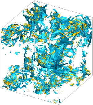
To illustrate the effects of large-scale thermal forcing and vibrational relaxation on the compression and expansion motions in the presently simulated flows, the instantaneous isosurfaces and contours of $\theta /\theta ^\prime$ for the $M_t \approx 0.22$ and $0.68$ cases are illustrated in figures 2, 3, 4 and 5. As shown in figure 2(a,b), for cases $\textrm {I}_2$ and $\textrm {I}_3$, both the strong compression and expansion regions are fragmentized sheet-like structures. The fragmentized sheet-like structures are more clear in the instantaneous contours of $\theta /\theta ^\prime$ (figure 3a,b). It is a distinctive compressible turbulent structure which is not reported in the prior literature, and is attributed to the combined effects of large-scale thermal forcing and vibrational relaxation. In our previous work on compressible isotropic turbulence in vibrational non-equilibrium (Zheng et al. Reference Zheng, Wang, Noack, Li, Wan and Chen2020), when the large-scale thermal forcing is excluded, both the strong compression and expansion regions are blob-like structures for the weakly compressible turbulence with $M_t \approx 0.44$. For case $\textrm {I}_4$ (figures 2c and 3c), as $\langle K_\tau \rangle$ increases to 9.80, the fragmentized sheet-like structures are replaced by the blob-like structures. In this case, the strong compression region is larger in size. For case $\textrm {I}_6$ (figures 2d and 3d), the flow compressibility is further enhanced. The percentage of volume occupied by the strong compression region is obviously larger than that by the strong expansion region. The structures in the former region are relatively flat and larger in size, while the latter region is characterized by the blob-like structures. For the $M_t \approx 0.68$ cases with different $\langle K_\tau \rangle$ and $\theta _v$ values, the instantaneous isosurfaces and contours of $\theta /\theta ^\prime$ are similar (figures 4 and 5). In these cases, the strong compression and expansion regions are respectively populated by the ‘shocklets’ and blob-like structures.

Figure 2. Instantaneous isosurfaces of normalized dilatation. (a) Case $\textrm {I}_2$, (b) case $\textrm {I}_3$, (c) case $\textrm {I}_4$ and (d) case $\textrm {I}_6$. Here $M_t \approx 0.22$.

Figure 3. Instantaneous contours of normalized dilatation. (a) Case $\textrm {I}_2$, (b) case $\textrm {I}_3$, (c) case $\textrm {I}_4$ and (d) case $\textrm {I}_6$. Here $M_t \approx 0.22$.

Figure 4. Instantaneous isosurfaces of normalized dilatation. (a) Case $\textrm {II}_2$, (b) case $\textrm {II}_6$. Here $M_t \approx 0.68$.

Figure 5. Instantaneous contours of normalized dilatation. (a) Case $\textrm {II}_2$, (b) case $\textrm {II}_6$. Here $M_t \approx 0.68$.

As shown in figures 4 and 5, the strong compression structures in these cases are relatively thicker, compared with our previous results for $M_t \approx 1.0$ (Zheng et al. Reference Zheng, Wang, Noack, Li, Wan and Chen2020). There is some literature about the estimation of shock thickness, such as Samtaney et al. (Reference Samtaney, Pullin and Kosović2001) and Donzis (Reference Donzis2012). For example, Donzis (Reference Donzis2012) mentioned that under laminar conditions, the normalized shock thickness could be written as

(4.1)\begin{equation} \frac{\delta_l}{\eta} \approx \frac{M_t}{Re_\lambda^{1/2}{\rm \Delta} M}, \end{equation}

where ${\rm \Delta} M = M -1$ and $\eta$ is the Kolmogorov scale. Under turbulent conditions, the shock thickness is essentially a random variable. The mean shock thickness can be given as

(4.2)\begin{equation} \frac{\langle \delta_l \rangle}{\eta} \approx \frac{M_t}{Re_\lambda^{1/2}{\rm \Delta} M}\left[1+\frac{1}{3}\frac{M_t^2}{{\rm \Delta} M^2}+\cdots\right]. \end{equation}

However, the present observations reveal that for the compressible turbulence in vibrational non-equilibrium, the shock thickness is closely related to the vibrational relaxation. The approximate relationship between the shock thickness and other parameters (e.g. $M_t$, $Re_\lambda$ and $\langle K_\tau \rangle$) is still not clear, and further investigations on the topic are required.

Figure 6 illustrates the compensated velocity spectrum $E^u(k)\epsilon ^{-2/3}k^{5/3}$ for the $M_t \approx 0.22$ and $0.68$ cases, where the velocity spectrum $E^u(k)$ satisfies $\int _0^\infty E^u(k)\,\textrm {d} k = \langle \boldsymbol{u}^2\rangle /2$. An inertial range of the velocity spectrum is observed in the range of $0.05 \lesssim k\eta \lesssim 0.2$ with a plateau about 2.0, which is larger than the widely accepted Kolmogorov constant of approximately 1.6. This deviation may result from the ‘bottleneck effect’ due to the limited $Re_\lambda$ (Gotoh & Fukayama Reference Gotoh and Fukayama2001; Dobler et al. Reference Dobler, Haugen, Yousef and Brandenburg2003). As mentioned in Donzis & Sreenivasan (Reference Donzis and Sreenivasan2010), the spectral bump decreases slowly with $Re_\lambda$ and became negligible only for $Re_\lambda$ greater than $\mathcal {O}(10^5)$. Furthermore, the compensated spectra of density and temperatures (i.e. $E^\rho (k)k^{5/3}/(\rho )_{rms}^2$, $E^{T_{tr}}(k)k^{5/3}/(T_{tr})_{rms}^2$ and $E^{T_{v}}(k)k^{5/3}/(T_{v})_{rms}^2$) are shown in figure 7, where $E^\rho (k)$, $E^{T_{tr}}(k)$ and $E^{T_v}(k)$ satisfy $\int _0^\infty E^\rho (k)\,\textrm {d} k = (\rho )_{rms}^2$, $\int _0^\infty E^{T_{tr}}(k)\,\textrm {d} k = (T_{tr})_{rms}^2$ and $\int _0^\infty E^{T_{v}}(k)\,\textrm {d} k = (T_{v})_{rms}^2$, respectively. The spectra of $\rho$, $T_{tr}$ and $T_{v}$ exhibit the $k^{-5/3}$ scaling for both the $M_t \approx 0.22$ and $0.68$ cases; a plateau at intermediate wavenumbers is apparent. For the stationary compressible isotropic turbulence without vibrational excitation and large-scale thermal forcing (Donzis & Jagannathan Reference Donzis and Jagannathan2013; Wang, Gotoh & Watanabe Reference Wang, Gotoh and Watanabe2017), the pressure, density and temperature spectra follow a scale of $k^{-5/3}$ in a range of $M_t$. In addition, the fluctuations at high wavenumbers for the weakly compressible turbulence ($M_t \approx 0.1$) are much smaller than those for the highly compressible turbulence ($M_t \approx 0.6$), especially in the spectra of pressure and density. However, in the presently simulated flows the compensated spectra of density and temperature for the $M_t \approx 0.22$ and $0.68$ cases are close to each other (figure 7), which suggests that the $M_t$ effect is negligible. The difference with the observations by Donzis & Jagannathan (Reference Donzis and Jagannathan2013) and Wang et al. (Reference Wang, Gotoh and Watanabe2017) could be attributed to the fact that the large-scale thermal forcing enhances the flow compressibility and fluctuation of thermodynamic variables at high wavenumbers.

Figure 6. Compensated spectra of velocity for (a) $M_t \approx 0.22$ and (b) $M_t \approx 0.68$ cases.

Figure 7. Compensated spectra of (a,d) density, (b,e) translational–rotational temperature and (c,f) vibrational temperature. Here, (a–c) $M_t \approx 0.22$ and (d–f) $M_t \approx 0.68$.

To reveal the effects of $M_t$, large-scale thermal forcing and vibrational relaxation on the pressure fluctuation, figure 8 presents the compensated spectra of pressure and its solenoidal and dilatational components. For both the $M_t \approx 0.22$ and $0.68$ cases, the spectra of solenoidal pressure component overlap roughly each other, and exhibit a $k^{-5/3}$ scaling at intermediate wavenumbers. In other words, the fluctuation of solenoidal pressure component is almost insensitive to the effects of $M_t$, large-scale thermal forcing and vibrational relaxation. Note that, the $k^{-5/3}$ scaling for the spectrum of the solenoidal (incompressible) pressure component was observed in a large number of previous studies, such as Vedula & Yeung (Reference Vedula and Yeung1999), Gotoh & Rogallo (Reference Gotoh and Rogallo1999), Donzis & Jagannathan (Reference Donzis and Jagannathan2013) and Wang et al. (Reference Wang, Gotoh and Watanabe2017). However, according to Kolmogorov's theory, the pressure spectrum in an incompressible turbulence should follow the $k^{-7/3}$ scaling. Gotoh & Fukayama (Reference Gotoh and Fukayama2001) suggested the $k^{-7/3}$ scaling with $Re_\lambda \geq 284$ in the numerical simulations of statistically steady homogeneous turbulence, while Tsuji & Ishihara (Reference Tsuji and Ishihara2003) found the $k^{-7/3}$ scaling with $Re_\lambda \geq 600$ in the experimental results of pressure fluctuation in a turbulent jet. Meldi & Sagaut (Reference Meldi and Sagaut2013) further revealed that the $k^{-7/3}$ scaling could be observed only with $Re_\lambda = O(10^4)$ in the numerical simulations of freely decaying homogeneous isotropic turbulence. Wang et al. (Reference Wang, Gotoh and Watanabe2017) found the $k^{-7/3}$ scaling in the pressure spectrum at the beginning of the inertial range for the weakly compressible isotropic turbulence with $M_t \leq 0.3$ and $Re_\lambda \approx 350$. Essentially, the exact threshold value of $Re_\lambda$ for the $k^{-7/3}$ scaling is not confirmed, rather dependent on specific turbulence. The present $k^{-5/3}$ scaling for the spectra of solenoidal pressure component should be attributed to the finite-Reynolds-number effect ($Re_\lambda \approx 157.5$ for the present simulations).

Figure 8. Compensated spectra of pressure and its solenoidal and dilatational components. Here, (a–c) $M_t \approx 0.22$ and (d–f) $M_t \approx 0.68$.

For the $M_t \approx 0.22$ cases, because of the large-scale thermal forcing, the fluctuations of pressure and its dilatational component at low wavenumbers are much larger than their counterparts for the $M_t \approx 0.68$ cases (figure 8). For cases $\textrm {I}_1 \text {--} \textrm {I}_3$, the fluctuations of pressure and its dilatational component do not differ much at low wavenumbers, while the fluctuation of dilatational pressure component decreases sharply with increasing wavenumbers. The spectra of pressure and its solenoidal component overlap approximately in the range of $k\eta \geq 0.1$. In these cases, the fluctuation of pressure at intermediate and high wavenumbers is dominated by the solenoidal component (figure 8a,b). For cases $\textrm {I}_4$ ($\langle K_\tau \rangle = 9.80$), the fluctuation of pressure at full wavenumbers is largely dominated by the dilatational component, with a slight departure in the range of $0.1 \leq k/\eta \leq 0.7$. Furthermore, the fluctuation of pressure at high wavenumbers in this case is much larger than that in the former three cases (figure 8b). Similar observations are made for cases $\textrm {I}_5$ and $\textrm {I}_6$ (figure 8c). With the increase of $\theta _v$, the fluctuations of pressure and its dilatational component at full wavenumbers increase, and the departure at intermediate wavenumbers shrinks. The above observations agree well with results in table 6, where $p^D_{rms}/p^S_{rms}$ increases from 2.59 to 4.82 with $\theta _v$ varying from 1.0 to 5.0 (cases $\textrm {I}_2$, $\textrm {I}_5$, $\textrm {I}_6$). For the $M_t \approx 0.68$ cases, the large-scale thermal forcing does not increase the fluctuation of pressure or its dilatational component at low wavenumbers. At intermediate wavenumbers, the spectra of pressure and its dilatational component exhibit roughly the $k^{-5/3}$ scaling. The fluctuation of dilatational pressure component is comparable with the solenoidal component for case $\textrm {II}_1$ (figure 8d). As $\langle K_\tau \rangle$ increases from 0.19 to 7.98, the fluctuation of dilatational pressure component decreases gradually, which agrees well with the observation in table 7, where $p^D_{rms}/p^S_{rms}$ decreases from 1.04 to 0.76 (cases $\textrm {II}_1 \text {--} \textrm {II}_4$). For cases $\textrm {II}_5$ and $\textrm {II}_6$, the spectra of solenoidal and dilatational components overlap roughly each other at low and intermediate wavenumbers (figure 8f). Furthermore, different from the $M_t \approx 0.22$ cases, the fluctuation of pressure at high wavenumbers ($k\eta \geq 0.8$) is mainly dominated by the dilatational component for the $M_t \approx 0.68$ cases.

As mentioned in § 3, $\chi (= \langle p \rangle \gamma _r M_t (u_{rms}^D/u^\prime )/p^D_{rms})$ is close to 1.0 for both the $M_t \approx 0.22$ and $0.68$ cases (tables 5–8), i.e. satisfying the weak form of acoustic equilibrium hypothesis. But how about the strong form of acoustic equilibrium hypothesis? Figure 9 presents the compensated spectra of dilatational velocity and pressure components (i.e. $2.0\gamma _r \langle \rho \rangle \langle p \rangle E^{u^D}(k)k^{-5/3}$ and $E^{p^D}(k)k^{-5/3}$) for the $M_t \approx 0.22$ and $0.68$ cases. Obviously, the compensated spectra of dilatational velocity component are closely related to the vibrational relaxation for the $M_t \approx 0.22$ cases. For cases $\textrm {I}_1 \text {--} \textrm {I}_3$, the two compensated spectra overlap at low wavenumbers, and begin to deviate at intermediate and high wavenumbers ($k\eta \geq 0.1$) (figure 9a). For cases $\textrm {I}_4 \text {--} \textrm {I}_6$, although the two compensated spectra do not overlap exactly at intermediate and high wavenumbers, they are close to each other and their trends are consistent (figure 9b). It reveals that for the $M_t \approx 0.22$ cases, the strong acoustic equilibrium hypothesis is valid only at low wavenumbers when the vibrational relaxation effect is significant. When the vibrational relaxation effect weakens ($\langle K_\tau \rangle$ or $\theta _v$ is large enough), the strong acoustic equilibrium hypothesis is approximately valid at all wavenumbers. For the $M_t \approx 0.68$ cases with different $\langle K_\tau \rangle$ and $\theta _v$ values, the two compensated spectra almost collapse at all wavenumbers (figure 9c,d). The observations suggest that the strong acoustic equilibrium hypothesis is valid for the $M_t \approx 0.68$ cases in despite of the vibrational relaxation.

Figure 9. Compensated spectra of dilatational velocity and pressure components. Note that, $H[E^{u^D}(k)] = 2.0\gamma _r \langle \rho \rangle \langle p \rangle E^{u^D}(k)k^{-5/3}$, $F[E^{p^D}(k)] = E^{p^D}(k)k^{-5/3}$. Here, (a,b) $M_t \approx 0.22$ and (c,d) $M_t \approx 0.68$.

5. Dissipation of internal energy fluctuations

From (2.2) and (2.3), the governing equations for internal energy and its translational–rotational component per unit mass ($e$ and $e_{tr}$) can be derived as

(5.1)$$\begin{gather} \frac{\partial{\rho e}}{\partial{t}} + \frac{\partial{\rho e u_j}}{\partial{x_j}}= \frac{1}{\alpha} \frac{\partial}{\partial{x_j}}\left(\kappa_{tr} \frac{\partial{T_{tr}}}{\partial{x_j}} + \kappa_v \frac{\partial{T_v}}{\partial{x_j}} \right) + \frac{1}{Re}\sigma_{ij}\frac{\partial{u_i}}{\partial{x_j}} -p\theta + \mathcal{F}_W, \end{gather}$$

(5.2)$$\begin{gather}\frac{\partial{\rho e_{tr}}}{\partial{t}} + \frac{\partial{\rho e_{tr} u_j}}{\partial{x_j}}= \frac{1}{\alpha} \frac{\partial}{\partial{x_j}}\left(\kappa_{tr} \frac{\partial{T_{tr}}}{\partial{x_j}} \right) + \frac{1}{Re}\sigma_{ij}\frac{\partial{u_i}}{\partial{x_j}} -p\theta + \mathcal{F}_W - \frac{E_v^*-E_v}{\tau_v}, \end{gather}$$

where $\mathcal {F}_W = - \varLambda + \mathcal {F}_I$ represents effects of the cooling function and the large-scale thermal forcing.

The translational–rotational energy can be decomposed into a spatially averaged component $e_{tr_0}(= \langle e_{tr} \rangle )$ and a fluctuation component $e_{tr_1}$, i.e. $e_{tr} = e_{tr_0} + e_{tr_1}$. The governing equation for the variance of translational–rotational energy $(\langle e_{tr_1}^2 \rangle )$ can be derived by taking a dot product of the translational–rotational energy governing equation (5.2) with $e_{tr_1}$ and spatially averaging, as

(5.3)\begin{align} \frac{\partial{\langle e_{tr_1}^2 \rangle }}{\partial{t}} &= \left\langle (e_{tr_1}^2 - \frac{4}{5}e_{tr}e_{tr_1})\theta \right\rangle - \left\langle \kappa_{tr}\frac{\partial T_{tr}}{\partial{x_j}} \frac{\partial}{\partial{x_j}} \left(\frac{2e_{tr_1}}{\rho\alpha}\right)\right\rangle + \left\langle \frac{2e_{tr_1}}{Re \rho} \sigma_{ij} \frac{\partial u_i}{\partial x_j} \right\rangle \nonumber\\ &\quad - \left\langle \frac{2e_{tr_1}}{\rho} \frac{E_v^*-E_v}{\tau_v} \right\rangle + \left\langle \frac{2e_{tr_1}}{\rho} F_W\right\rangle ={-} \langle \mathcal{C}_{e_{tr}} \rangle + \langle \mathcal{C}_{e_{tr}}^{inj} \rangle. \end{align}

Here, the total change rate of translational–rotational energy fluctuation can be decomposed as $\langle \mathcal {C}_{e_{tr}} \rangle = \langle \mathcal {C}_{e_{tr}}^\theta \rangle + \langle \mathcal {C}_{e_{tr}}^\kappa \rangle + \langle \mathcal {C}_{e_{tr}}^\mu \rangle + \langle \mathcal {C}_{e_{tr}}^\tau \rangle$. The change rates due to the effects of dilatation, thermal conduction, viscosity and vibrational relaxation are respectively denoted as

(5.4a,b) \begin{gather}\langle \mathcal{C}_{e_{tr}}^\theta \rangle ={-} \left\langle (e_{tr_1}^2 - \frac{4}{5}e_{tr}e_{tr_1})\theta \right\rangle,\quad \langle \mathcal{C}_{e_{tr}}^\kappa \rangle = \left\langle \kappa_{tr}\frac{\partial T_{tr}}{\partial{x_j}} \frac{\partial}{\partial{x_j}} \left(\frac{2e_{tr_1}}{\rho\alpha}\right)\right\rangle,\end{gather}

(5.5a,b) \begin{gather}\langle \mathcal{C}_{e_{tr}}^\mu \rangle ={-} \left\langle \frac{2e_{tr_1}}{Re \rho} \sigma_{ij} \frac{\partial u_i}{\partial x_j} \right\rangle \quad \textrm{and} \quad \langle \mathcal{C}_{e_{tr}}^\tau \rangle = \left\langle \frac{2e_{tr_1}}{\rho} \frac{E_v^*-E_v}{\tau_v} \right\rangle.\end{gather}

The $\langle \mathcal {C}_{e_{tr}}^{inj} \rangle = \langle (2e_{tr_1}/\rho ) F_W \rangle$ represents the injection of translational–rotational energy fluctuation by the cooling function and large-scale thermal forcing.

Similarly, the governing equation for the variance of vibrational energy is derived as

(5.6)\begin{equation} \frac{\partial{\langle e_{v_1}^2 \rangle }}{\partial{t}} = \langle e_{v_1}^2\theta \rangle - \left\langle \kappa_{v}\frac{\partial T_{v}}{\partial{x_j}} \frac{\partial}{\partial{x_j}} \left(\frac{2e_{v_1}}{\rho\alpha}\right)\right\rangle + \left\langle \frac{2e_{v_1}}{\rho} \frac{E_v^*-E_v}{\tau_v} \right\rangle ={-} \langle \mathcal{C}_{e_{v}} \rangle, \end{equation}

where $e_{v_1} = e_{v} - e_{v_0}$ and $e_{v_0} = \langle e_{v} \rangle$. The total change rate of vibrational energy fluctuation is decomposed as $\langle \mathcal {C}_{e_{v}} \rangle = \langle \mathcal {C}_{e_{v}}^\theta \rangle + \langle \mathcal {C}_{e_{v}}^\kappa \rangle + \langle \mathcal {C}_{e_{v}}^\tau \rangle$. The change rates due to the effects of dilatation, thermal conduction and vibrational relaxation are respectively

(5.7a–c)\begin{align} \langle \mathcal{C}_{e_{v}}^\theta \rangle ={-}\langle e_{v_1}^2\theta \rangle,\quad \langle \mathcal{C}_{e_{v}}^\kappa \rangle = \left\langle \kappa_{v}\frac{\partial T_{v}}{\partial{x_j}} \frac{\partial}{\partial{x_j}} \left(\frac{2e_{v_1}}{\rho\alpha}\right)\right\rangle \quad \textrm{and} \quad \langle \mathcal{C}_{e_{v}}^\tau \rangle ={-}\left\langle \frac{2e_{v_1}}{\rho} \frac{E_v^*-E_v}{\tau_v} \right\rangle. \end{align}

The change rates of the translational–rotational and vibrational energy fluctuations are given in tables 9 and 10 for the $M_t \approx 0.22$ cases, and in tables 11 and 12 for the $M_t \approx 0.68$ cases. The total change rates of the translational–rotational and vibrational energy fluctuations for the $M_t \approx 0.22$ and $0.68$ cases are given in table 13. For the translational–rotational energy fluctuation, from (5.3), the total change rate $\langle \mathcal {C}_{e_{tr}} \rangle$ is positive. As shown in tables 9–12, $\langle \mathcal {C}_{e_{tr}}^\theta \rangle / \langle \mathcal {C}_{e_{tr}} \rangle$ and $\langle \mathcal {C}_{e_{tr}}^\mu \rangle / \langle \mathcal {C}_{e_{tr}} \rangle$ are negligibly small, while $\langle \mathcal {C}_{e_{tr}}^\kappa \rangle / \langle \mathcal {C}_{e_{tr}} \rangle$ is larger than $\langle \mathcal {C}_{e_{tr}}^\tau \rangle / \langle \mathcal {C}_{e_{tr}} \rangle$. It suggests that for both the $M_t \approx 0.22$ and $0.68$ cases, on spatial average, the change rates of translational–rotational energy fluctuation due to the dilatation and viscosity are negligible; the dissipation mainly comes from the effects of thermal conduction and vibrational relaxation, while the former plays a major role. As shown in table 13, $\langle \mathcal {C}_{e_{tr}} \rangle$ and $\langle \mathcal {C}_{e_{v}} \rangle$ for the $M_t \approx 0.22$ cases are much larger than their counterparts for the $M_t \approx 0.68$ cases. It implies that the large-scale thermal forcing has more significant impacts for the $M_t \approx 0.22$ cases, which agrees well with the observations in § 4.

Table 9. The ratio of dissipation rates for translational–rotational and vibrational energy fluctuations. Considering $\langle K_\tau \rangle$ effects. Here $M_t \approx 0.22$.

Table 10. The ratio of dissipation rates for translational–rotational and vibrational energy fluctuations. Considering $\theta _v$ effects. Here $M_t \approx 0.22$.

Table 11. The ratio of dissipation rates for translational–rotational and vibrational energy fluctuations. Considering $\langle K_\tau \rangle$ effects. Here $M_t \approx 0.68$.

Table 12. The ratio of dissipation rates for translational–rotational and vibrational energy fluctuations. Considering $\theta _v$ effects. Here $M_t \approx 0.68$.

Table 13. Total change rates of translational–rotational and change rate of vibrational energy fluctuations due to vibrational relaxation for the $M_t \approx 0.22$ and $0.68$ cases.

For the $M_t \approx 0.22$ cases, $\langle \mathcal {C}_{e_{tr}}^\kappa \rangle /\langle \mathcal {C}_{e_{tr}} \rangle$ keeps almost constant ($\approx 0.776$, table 9) for cases $\textrm {I}_1\text {--}\textrm {I}_4$, and increases from 0.790 to 0.962 with $\theta _v$ varying from 1.0 to 5.0 (cases $\textrm {I}_2, \textrm {I}_5, \textrm {I}_6$, table 10). Furthermore, $\langle \mathcal {C}_{e_{tr}}^\tau \rangle /\langle \mathcal {C}_{e_{tr}} \rangle$ increases slightly from 0.205 to 0.232 as $\langle K_\tau \rangle$ increases from 0.16 to 9.80, while decreasing sharply from 0.208 to 0.072 with $\theta _v$ varying from 1.0 to 5.0. For the $M_t \approx 0.68$ cases, $\langle \mathcal {C}_{e_{tr}}^\kappa \rangle /\langle \mathcal {C}_{e_{tr}} \rangle \approx 0.739$ for different cases (tables 11 and 12). The $\langle \mathcal {C}_{e_{tr}}^\tau \rangle /\langle \mathcal {C}_{e_{tr}} \rangle \approx 0.277$ with $\langle K_\tau \rangle \approx 0.19$. The $\langle \mathcal {C}_{e_{tr}}^\tau \rangle /\langle \mathcal {C}_{e_{tr}} \rangle$ wanes from 0.349 to 0.280 as $\langle K_\tau \rangle$ increases from 0.86 to 7.98 (table 11), and declines sharply from 0.349 to 0.089 with $\theta _v$ varying from 1.0 to 5.0 (table 12). Note that, for the $M_t \approx 0.68$ cases, the dilatation term also plays a considerable role with increasing $\theta _v$; for instance, $\langle \mathcal {C}_{e_{tr}}^\theta \rangle /\langle \mathcal {C}_{e_{tr}} \rangle$ is about 0.105 for case $\textrm {II}_6$. The observations indicate that the variation of $\langle \mathcal {C}_{e_{tr}}^\kappa \rangle /\langle \mathcal {C}_{e_{tr}} \rangle$ depends mainly on $\theta _v$ for the $M_t \approx 0.22$ cases, and is almost insensitive to $\langle K_\tau \rangle$ and $\theta _v$ for the $M_t \approx 0.68$ cases. Furthermore, for both the $M_t \approx 0.22$ and $0.68$ cases, $\langle \mathcal {C}_{e_{tr}}^\tau \rangle /\langle \mathcal {C}_{e_{tr}} \rangle$ has a limited connection with $\langle K_\tau \rangle$, while highly depends on $\theta _v$. As $\theta _v$ increases, the dissipation of translational–rotational energy fluctuation due to the vibrational relaxation loses its significance rapidly.

For the vibrational energy fluctuation (5.6), the total change rate $\langle \mathcal {C}_{e_{v}} \rangle$ approximately equals zero. Because of the equilibrium departure, an exchange between the translational–rotational and vibrational energies takes place via vibrational relaxation. Consequently, the change rate due to the vibrational relaxation ($\langle \mathcal {C}_{e_{v}}^\tau \rangle$) is negative (table 13). That is, the vibrational relaxation enhances essentially the vibrational energy fluctuation. From tables 9–12, $\langle \mathcal {C}_{e_{v}}^\theta \rangle /(-\langle \mathcal {C}_{e_{v}}^\tau \rangle )$ roughly equals 0.0, while $\langle \mathcal {C}_{e_{v}}^\kappa \rangle /(-\langle \mathcal {C}_{e_{v}}^\tau \rangle )$ is close to 1.0. It suggests that the change rate of vibrational energy fluctuation due to the dilatation is nearly negligible, while the dissipation of vibrational energy fluctuation due to the thermal conduction is roughly equivalent to the production owing to the vibrational relaxation.

To investigate the effect of flow compressibility on the change rate of internal energy fluctuations, we define the parameters

(5.8a,b)$$\begin{gather} \mathcal{C}_{e_{tr}}^\theta ={-}\left(e_{tr_1}^2 - \frac{4}{5}e_{tr}e_{tr_1}\right)\theta,\quad \mathcal{C}_{e_{tr}}^\kappa = \kappa_{tr}\frac{\partial T_{tr}}{\partial{x_j}} \frac{\partial}{\partial{x_j}} \left(\frac{2e_{tr_1}}{\rho\alpha}\right), \end{gather}$$

(5.9a,b)$$\begin{gather}\mathcal{C}_{e_{tr}}^\mu ={-} \frac{2e_{tr_1}}{Re \rho} \sigma_{ij} \frac{\partial u_i}{\partial x_j} \quad \textrm{and} \quad \mathcal{C}_{e_{tr}}^\tau = \frac{2e_{tr_1}}{\rho} \frac{E_v^*-E_v}{\tau_v}, \end{gather}$$

for the translational–rotational energy fluctuation, and

(5.10a–c)\begin{equation} \mathcal{C}_{e_{v}}^\theta ={-}e_{v_1}^2\theta,\quad \mathcal{C}_{e_{v}}^\kappa = \kappa_{v}\frac{\partial T_{v}}{\partial{x_j}} \frac{\partial}{\partial{x_j}} \left(\frac{2e_{v_1}}{\rho\alpha}\right)\quad \textrm{and} \quad \mathcal{C}_{e_{v}}^\tau ={-}\frac{2e_{v_1}}{\rho} \frac{E_v^*-E_v}{\tau_v}, \end{equation}

for the vibrational energy fluctuation. The spatially averaged $(\mathcal {C}_{e_{tr}}^\theta -\langle \mathcal {C}_{e_{tr}}^\theta \rangle )/\langle \mathcal {C}_{e_{tr}}\rangle$, $(\mathcal {C}_{e_{tr}}^\kappa -\langle \mathcal {C}_{e_{tr}}^\kappa \rangle )/\langle \mathcal {C}_{e_{tr}}\rangle$, $(\mathcal {C}_{e_{tr}}^\mu -\langle \mathcal {C}_{e_{tr}}^\mu \rangle )/\langle \mathcal {C}_{e_{tr}}\rangle$, $(\mathcal {C}_{e_{tr}}^\tau -\langle \mathcal {C}_{e_{tr}}^\tau \rangle )/\langle \mathcal {C}_{e_{tr}}\rangle$, $(\mathcal {C}_{e_{v}}^\theta -\langle \mathcal {C}_{e_{v}}^\theta \rangle )/(-\langle \mathcal {C}_{e_{v}}^\tau \rangle )$, $(\mathcal {C}_{e_{v}}^\kappa -\langle \mathcal {C}_{e_{v}}^\kappa \rangle )/(-\langle \mathcal {C}_{e_{v}}^\tau \rangle )$ and $(\mathcal {C}_{e_{v}}^\tau -\langle \mathcal {C}_{e_{v}}^\tau \rangle )/(-\langle \mathcal {C}_{e_{v}}^\tau \rangle )$ conditioned on $\theta /\theta ^\prime$ are presented in figure 10. Here, only the $M_t \approx 0.68$ cases are considered owing to their notable flow compressibility.

Figure 10. Spatially averaged (a) $(\mathcal {C}_{e_{tr}}^\theta -\langle \mathcal {C}_{e_{tr}}^\theta \rangle )/\langle \mathcal {C}_{e_{tr}}\rangle$, (b) $(\mathcal {C}_{e_{tr}}^\kappa -\langle \mathcal {C}_{e_{tr}}^\kappa \rangle )/\langle \mathcal {C}_{e_{tr}}\rangle$ (with symbol), $(\mathcal {C}_{e_{tr}}^\mu -\langle \mathcal {C}_{e_{tr}}^\mu \rangle )/\langle \mathcal {C}_{e_{tr}}\rangle$ (solid line), (c) $(\mathcal {C}_{e_{tr}}^\tau -\langle \mathcal {C}_{e_{tr}}^\tau \rangle )/\langle \mathcal {C}_{e_{tr}}\rangle$, (d) $(\mathcal {C}_{e_{v}}^\theta -\langle \mathcal {C}_{e_{v}}^\theta \rangle )/(-\langle \mathcal {C}_{e_{v}}^\tau \rangle )$, (e) $(\mathcal {C}_{e_{v}}^\kappa -\langle \mathcal {C}_{e_{v}}^\kappa \rangle )/(-\langle \mathcal {C}_{e_{v}}^\tau \rangle )$ and (f) $(\mathcal {C}_{e_{v}}^\tau -\langle \mathcal {C}_{e_{v}}^\tau \rangle )/(-\langle \mathcal {C}_{e_{v}}^\tau \rangle )$ conditioned on $\theta /\theta ^\prime$. $M_t \approx 0.68$.

For the fluctuation of translational–rotational energy, as shown in figure 10(a), the $\langle (\mathcal {C}_{e_{tr}}^\theta -\langle \mathcal {C}_{e_{tr}}^\theta \rangle )/\langle \mathcal {C}_{e_{tr}}\rangle | \theta /\theta ^\prime \rangle$ is positive and increases rapidly in the compression region, while it is negative and decreases sharply in the expansion region. Note that in the range of $|\theta /\theta ^\prime | \leq 0.65$, the changes of $\langle (\mathcal {C}_{e_{tr}}^\theta -\langle \mathcal {C}_{e_{tr}}^\theta \rangle )/\langle \mathcal {C}_{e_{tr}}\rangle | \theta /\theta ^\prime \rangle$ are relatively small. Compared with the dilatation term, the dependence of other terms on $\theta /\theta ^\prime$ is much weaker. The $\langle (\mathcal {C}_{e_{tr}}^\kappa -\langle \mathcal {C}_{e_{tr}}^\kappa \rangle )/\langle \mathcal {C}_{e_{tr}}\rangle |\theta /\theta ^\prime \rangle$ rises with the increase of $\theta /\theta ^\prime$ magnitude in the compression and expansion regions (figure 10b). In the strong compression region ($\theta /\theta ^\prime \leq -2.0$), it is insensitive to $\langle K_\tau \rangle$, but enlarges with the increase of $\theta _v$. Beyond the strong compression region, the vibrational relaxation effect is negligibly small. For the $\langle (\mathcal {C}_{e_{tr}}^\mu -\langle \mathcal {C}_{e_{tr}}^\mu \rangle )/\langle \mathcal {C}_{e_{tr}}\rangle | \theta /\theta ^\prime \rangle$, the effects of flow compressibility and vibrational relaxation are weak. The $\langle (\mathcal {C}_{e_{tr}}^\mu -\langle \mathcal {C}_{e_{tr}}^\mu \rangle )/\langle \mathcal {C}_{e_{tr}}\rangle | \theta /\theta ^\prime \rangle$ for different cases roughly overlap each other and keep almost constant in the compression and expansion regions (figure 10b). Here, to distinguish the thermal conduction term from the viscosity term, the solid lines representing $\langle (\mathcal {C}_{e_{tr}}^\mu -\langle \mathcal {C}_{e_{tr}}^\mu \rangle )/\langle \mathcal {C}_{e_{tr}}\rangle | \theta /\theta ^\prime \rangle$ are offset by $-$1.0. For the $\langle (\mathcal {C}_{e_{tr}}^\tau -\langle \mathcal {C}_{e_{tr}}^\tau \rangle )/\langle \mathcal {C}_{e_{tr}}\rangle | \theta /\theta ^\prime \rangle$, their variances in the compression region are closely related to the vibrational relaxation. The $\langle (\mathcal {C}_{e_{tr}}^\tau -\langle \mathcal {C}_{e_{tr}}^\tau \rangle )/\langle \mathcal {C}_{e_{tr}}\rangle | \theta /\theta ^\prime \rangle$ are close for cases $\textrm {II}_1$ and $\textrm {II}_2$, being positive and enlarging with the increase of $\theta /\theta ^\prime$ magnitude in the compression region. The magnitude of $\langle (\mathcal {C}_{e_{tr}}^\tau -\langle \mathcal {C}_{e_{tr}}^\tau \rangle )/\langle \mathcal {C}_{e_{tr}}\rangle | \theta /\theta ^\prime \rangle$ is significantly suppressed with the increase of $\langle K_\tau \rangle$ and $\theta _v$ (figure 10c). For example, for cases $\mathrm {II}_3$ and $\mathrm {II}_4$, the $\langle (\mathcal {C}_{e_{tr}}^\tau -\langle \mathcal {C}_{e_{tr}}^\tau \rangle )/\langle \mathcal {C}_{e_{tr}}\rangle | \theta /\theta ^\prime \rangle$ is almost insensitive to $\theta /\theta ^\prime$. In the expansion region, however, no obvious dependence on the flow compressibility and vibrational relaxation is observed.

For the vibrational energy fluctuation, the $\langle (\mathcal {C}_{e_{v}}^\theta -\langle \mathcal {C}_{e_{v}}^\theta \rangle )/(-\langle \mathcal {C}_{e_{v}}^\tau \rangle ) |\theta /\theta ^\prime \rangle$ for different cases are positive and negative in the compression and expansion regions, respectively (figure 10d). Their magnitudes are amplified with the increase of $\theta /\theta ^\prime$ magnitude. The $\langle (\mathcal {C}_{e_{v}}^\kappa -\langle \mathcal {C}_{e_{v}}^\kappa \rangle )/(-\langle \mathcal {C}_{e_{v}}^\tau \rangle )| \theta /\theta ^\prime \rangle$ for different cases are insensitive to $\theta /\theta ^\prime$ and vibrational relaxation, keeping constant in the compression region except case $\textrm {II}_1$, while increasing slightly in the expansion region (figure 10e). As shown in figure 10(f), the $\langle (\mathcal {C}_{e_{v}}^\tau -\langle \mathcal {C}_{e_{v}}^\tau \rangle )/(-\langle \mathcal {C}_{e_{v}}^\tau \rangle ) | \theta /\theta ^\prime \rangle$ are close for cases $\textrm {II}_1$ and $\textrm {II}_2$, being negative in the compression region and positive in the expansion region. The dependence of $\langle (\mathcal {C}_{e_{v}}^\tau -\langle \mathcal {C}_{e_{v}}^\tau \rangle )/(-\langle \mathcal {C}_{e_{v}}^\tau \rangle ) | \theta /\theta ^\prime \rangle$ on the flow compressibility reduces greatly as $\langle K_\tau \rangle$ increases. For instance, the $\langle (\mathcal {C}_{e_{v}}^\tau -\langle \mathcal {C}_{e_{v}}^\tau \rangle )/(-\langle \mathcal {C}_{e_{v}}^\tau \rangle ) | \theta /\theta ^\prime \rangle$ is almost insensitive to the compressibility for cases $\textrm {II}_3$ and $\textrm {II}_4$. Note that, the dependency of $\langle (\mathcal {C}_{e_{v}}^\tau -\langle \mathcal {C}_{e_{v}}^\tau \rangle )/(-\langle \mathcal {C}_{e_{v}}^\tau \rangle ) | \theta /\theta ^\prime \rangle$ is enhanced sharply for case $\textrm {II}_6$, because the value of $(-\langle \mathcal {C}_{e_{v}}^\tau \rangle )$ for case $\textrm {II}_6$ is much smaller than other cases (table 13).

6. Transfer of internal energy fluctuation

The Favre filtering approach is employed to study the transfers of translational–rotational and vibrational energy fluctuations. The classically filtered field $\bar {f}$ is defined as $\bar {f}(\boldsymbol{x})\equiv \int \textrm {d}^3 \boldsymbol{r}G_l(\boldsymbol{r})f(\boldsymbol{x}+\boldsymbol{r})$. The $G_l(\boldsymbol{r}) \equiv l^{-3}G(\boldsymbol{r}/l)$ is the filter function, where $G(\boldsymbol{r})$ is a normalized window function and $l$ is the filter width. The Favre filtered field $\tilde {f}$ is defined as $\tilde {f} \equiv \overline {\rho f}/\bar {\rho }$. In the present study a top-hat filter is adopted, which is calculated by (Martin, Piomelli & Candler Reference Martin, Piomelli and Candler2000)

(6.1)\begin{equation} \bar{f}_i = \frac{1}{4n}\left( f_{i-n}+2\sum_{j=i-n+1}^{i+n-1} f_j+f_{i+n} \right), \end{equation}

where the filter width $l = 2n {\rm \Delta} x$.

The governing equation for the variance of filtered translational--rotational energy can be derived from (5.2) as

(6.2)\begin{align} \frac{\partial{\langle \tilde{e}_{tr_1}^2 \rangle }}{\partial{t}} &= \left\langle \tilde{e}_{tr_1}^2\theta_l - \frac{2 \tilde{e}_{tr_1}}{\bar{\rho}} \overline{p\theta} \right\rangle - \left\langle \overline{\kappa_{tr}\frac{\partial T_{tr}}{\partial{x_j}}} \frac{\partial}{\partial{x_j}} \left(\frac{2\tilde{e}_{tr_1}}{\bar{\rho}\alpha}\right)\right\rangle + \left\langle \frac{2\tilde{e}_{tr_1}}{Re\bar{\rho}}\overline{\sigma_{ij} \frac{\partial u_i}{\partial x_j}}\right\rangle \nonumber\\ &\quad -\left\langle \frac{2\tilde{e}_{tr_1}}{\bar{\rho}} \overline{\frac{E_v^*-E_v}{\tau_v}}\right\rangle + \left\langle \bar{\rho}(\widetilde{e_{tr_1}u_j} - \tilde{e}_{tr_1}\tilde{u}_j) \frac{\partial}{\partial x_j}(\frac{2\tilde{e}_{tr_1}}{\bar{\rho}}) \right\rangle + \left\langle \frac{2\tilde{e}_{tr_1}}{\bar{\rho}} \bar{F}_W \right\rangle \nonumber\\ &={-} \langle \varPhi_l^{e_{tr}} + D_l^{e_{tr}} + \varGamma_l^{e_{tr}} + \varPi_l^{e_{tr}} \rangle + \langle F_l^{e_{tr}} \rangle, \end{align}

where $\theta _l (= \partial \tilde {u}_j/\partial x_j)$ is the filtered velocity divergence. The dilatation term $\varPhi _l^{e_{tr}}$, thermal conduction and viscosity term $D_l^{e_{tr}}$, vibrational relaxation term $\varGamma _l^{e_{tr}}$, subgrid-scale (SGS) flux term $\varPi _l^{e_{tr}}$, and effects of large-scale thermal forcing and cooling function $F_l^{e_{tr}}$ can be respectively presented as

(6.3a,b)\begin{gather} \varPhi_l^{e_{tr}} ={-}\tilde{e}_{tr_1}^2\theta_l + \frac{2 \tilde{e}_{tr_1}}{\bar{\rho}} \overline{p\theta},\quad D_l^{e_{tr}} = \overline{\kappa_{tr}\frac{\partial T_{tr}}{\partial{x_j}}} \frac{\partial}{\partial{x_j}} \left(\frac{2\tilde{e}_{tr_1}}{\bar{\rho}\alpha}\right) - \frac{2\tilde{e}_{tr_1}}{Re\bar{\rho}}\overline{\sigma_{ij}\frac{\partial u_i}{\partial x_j}}, \end{gather}

(6.4a,b) \begin{gather} \varGamma_l^{e_{tr}} = \frac{2\tilde{e}_{tr_1}}{\bar{\rho}} \overline{\frac{E_v^*-E_v}{\tau_v}},\quad \varPi_l^{e_{tr}} ={-} \bar{\rho}(\widetilde{e_{tr_1}u_j} - \tilde{e}_{tr_1}\tilde{u}_j) \frac{\partial}{\partial{x_j}}\left(\frac{2\tilde{e}_{tr_1}} {\bar{\rho}}\right)\end{gather}

(6.5) \begin{gather}\textrm{and}\quad F_l^{e_{tr}} = \frac{2\tilde{e}_{tr_1}}{\bar{\rho}} \bar{F}_W. \end{gather}

Similarly, the governing equation for the variance of filtered vibrational energy can be derived from (2.4) as

(6.6) \begin{align} \frac{\partial{\langle \tilde{e}_{v_1}^2 \rangle }}{\partial{t}} &= \langle \tilde{e}_{v_1}^2\theta_l \rangle - \left\langle \overline{\kappa_{v} \frac{\partial T_{v}}{\partial{x_j}}} \frac{\partial}{\partial{x_j}} \left(\frac{2\tilde{e}_{v_1}}{\bar{\rho}\alpha}\right)\right\rangle + \left\langle \frac{2\tilde{e}_{v_1}}{\bar{\rho}} \overline{\frac{E_v^*-E_v}{\tau_v}}\right\rangle \nonumber\\ &\quad + \left\langle \bar{\rho}(\widetilde{e_{v_1}u_j} - \tilde{e}_{v_1}\tilde{u}_j) \frac{\partial}{\partial x_j}\left(\frac{2\tilde{e}_{v_1}}{\bar{\rho}}\right) \right\rangle ={-} \langle \varPhi_l^{e_{v}} + D_l^{e_{v}} + \varGamma_l^{e_{v}} + \varPi_l^{e_{v}} \rangle. \end{align}

The dilatation term $\varPhi _l^{e_{v}}$, thermal conduction term $D_l^{e_{v}}$, vibrational relaxation term $\varGamma _l^{e_{v}}$ and SGS flux term $\varPi _l^{e_{v}}$ can be respectively denoted as

(6.7a,b)$$\begin{gather} \varPhi_l^{e_{v}} ={-} \tilde{e}_{v_1}^2\theta_l,\quad D_l^{e_{v}} = \overline{\kappa_{v}\frac{\partial T_{v}}{\partial{x_j}}} \frac{\partial}{\partial{x_j}} \left(\frac{2\tilde{e}_{v_1}}{\bar{\rho}\alpha}\right), \end{gather}$$

(6.8a,b)$$\begin{gather}\varGamma_l^{e_{v}} ={-} \frac{2\tilde{e}_{v_1}}{\bar{\rho}} \overline{\frac{E_v^*-E_v}{\tau_v}}\quad \textrm{and}\quad \varPi_l^{e_{v}} ={-} \bar{\rho}(\widetilde{e_{v_1}u_j} - \tilde{e}_{v_1}\tilde{u}_j) \frac{\partial}{\partial x_j}\left(\frac{2\tilde{e}_{v_1}}{\bar{\rho}}\right). \end{gather}$$

6.1. Transfer of internal energy fluctuation

The dependence of $\langle \varPhi _l^{e_{tr}}+D_l^{e_{tr}}+\varGamma _l^{e_{tr}}+\varPi _l^{e_{tr}} \rangle / \langle \mathcal {C}_{e_{tr}} \rangle$, $\langle \varPhi _l^{e_{tr}} \rangle / \langle \mathcal {C}_{e_{tr}} \rangle$, $\langle D_l^{e_{tr}} \rangle / \langle \mathcal {C}_{e_{tr}} \rangle$, $\langle \varGamma _l^{e_{tr}} \rangle / \langle \mathcal {C}_{e_{tr}} \rangle$ and $\langle \varPi _l^{e_{tr}} \rangle / \langle \mathcal {C}_{e_{tr}} \rangle$ on $l/\eta$ are similar among the $M_t \approx 0.22$ cases. So are the $M_t \approx 0.68$ cases. Here, as shown in figure 11, the cases $\textrm {I}_2$ and $\textrm {II}_2$ are taken to be examples. The $\langle \varPhi _l^{e_{tr}}+D_l^{e_{tr}}+\varGamma _l^{e_{tr}}+\varPi _l^{e_{tr}} \rangle / \langle \mathcal {C}_{e_{tr}} \rangle$ approximately equals $1.0$ in the range of $l/\eta \leq 50.0$ (figure 11a,b). It indicates that the effect of large-scale forcing on the transfer of translational–rotational energy fluctuation is mainly localized in large-scale motions. The $\langle \varPhi _l^{e_{tr}} \rangle / \langle \mathcal {C}_{e_{tr}} \rangle$ increases in the range of $l/\eta \leq 50.0$ and decreases in $l/\eta > 50.0$ for case $\textrm {I}_2$. Similarly, $\langle \varPhi _l^{e_{tr}} \rangle / \langle \mathcal {C}_{e_{tr}} \rangle$ increases in $l/\eta \leq 70.0$ and decreases in $l/\eta > 70.0$ for case $\textrm {II}_2$. The observation suggests that on spatial average, the dilatation effect weakens the translational–rotational energy fluctuation in large-scale motions, and enhances it in small- and intermediate-scale motions. The $\langle D_l^{e_{tr}} \rangle / \langle \mathcal {C}_{e_{tr}} \rangle$ approximately equals 0.7 and 0.65 at $l/\eta \approx 1.92$ for cases $\textrm {I}_2$ and $\textrm {II}_2$, respectively, and decreases monotonously with $l/\eta$. The $\langle D_l^{e_{tr}} \rangle / \langle \mathcal {C}_{e_{tr}} \rangle$ approaches $0.0$ in $l/\eta \geq 60.0$ (figure 11a,b). That is, the thermal conduction and viscosity effects weaken the translational–rotational energy fluctuation, and mainly act on small- and intermediate-scale motions. The $\langle \varGamma _l^{e_{tr}} \rangle / \langle \mathcal {C}_{e_{tr}} \rangle$ keeps constant (${\approx }0.2$) in $l/\eta \leq 60.0$ for case $\textrm {I}_2$, and ${\approx }0.35$ in $l/\eta \leq 7.0$ for case $\textrm {II}_2$ (figure 11a,b), and reduces with $l/\eta$ beyond these ranges. It implies that the vibrational relaxation weakens the translational–rotational energy fluctuation, and acts mainly on large-scale motions for the $M_t \approx 0.22$ cases. The affected range is extended to intermediate- and large-scale motions for the $M_t \approx 0.68$ cases. Furthermore, the vibrational relaxation effect on the dissipation of translational–rotational energy fluctuation is stronger in the $M_t \approx 0.68$ cases. This observation is consistent with the results in tables 9–12, where $\langle \mathcal {C}_{e_{tr}}^\tau \rangle /\langle \mathcal {C}_{e_{tr}} \rangle$ values for the $M_t \approx 0.22$ cases are always smaller than their counterparts for the $M_t \approx 0.68$ cases. As shown in figure 11(a,b), $\langle \varPi _l^{e_{tr}} \rangle /\langle \mathcal {C}_{e_{tr}} \rangle \approx 0.5$ in $20 \leq l/\eta \leq 80$ for cases $\textrm {I}_2$ and $\textrm {II}_2$, suggesting that about half of the translational–rotational energy fluctuations cascade from large- to small-scale motions in this range. Obviously, in this range ($20 \leq l/\eta \leq 80$), the dilatation and vibrational relaxation terms (i.e. $\langle \varPhi _l^{e_{tr}} \rangle /\langle \mathcal {C}_{e_{tr}} \rangle$ and $\langle \varPi _l^{e_{tr}} \rangle /\langle \mathcal {C}_{e_{tr}} \rangle$) also play a significant role, and dissipate another half of the translational–rotational energy fluctuation. These observations are different from the previous results about cascades of thermal parameters in the compressible isotropic turbulence without vibrational excitation. Wang et al. (Reference Wang, Wan, Chen, Xie, Wang and Chen2019) investigated the cascades of temperature and entropy fluctuations of the stationary compressible isotropic turbulence with large-scale thermal forcing in the absence of vibrational relaxation. They found that $\langle \varPi _l^{T} \rangle /\epsilon _{T} \approx 1.0$ and $\langle \varPi _l^{s} \rangle /\epsilon _{s} \approx 1.0$ in $30 \leq l/\eta \leq 100$ for both the $M_t \approx 0.2$ and $0.6$ cases. That is, all of the temperature and entropy fluctuations cascade approximately from large- to small-scale motions in this range, while the dilatation term plays a negligible role in dissipating the temperature and entropy fluctuations.

Figure 11. Dependence on $l/\eta$ of $\langle \varPhi _l^{e_{tr}} \rangle /\langle \mathcal {C}_{e_{tr}} \rangle$, $\langle D_l^{e_{tr}} \rangle /\langle \mathcal {C}_{e_{tr}} \rangle$, $\langle \varGamma _l^{e_{tr}} \rangle /\langle \mathcal {C}_{e_{tr}} \rangle$, $\langle \varPi _l^{e_{tr}} \rangle /\langle \mathcal {C}_{e_{tr}} \rangle$ and $\langle \varPhi _l^{e_{tr}} + D_l^{e_{tr}} + \varGamma _l^{e_{tr}} + \varPi _l^{e_{tr}} \rangle /\langle \mathcal {C}_{e_{tr}} \rangle$. (a) Case $\textrm {I}_2$, (b) case $\textrm {II}_2$.

Figure 12 shows the dependence on $l/\eta$ of $\langle \varPhi _l^{e_{v}}+D_l^{e_{v}}+\varGamma _l^{e_{v}}+\varPi _l^{e_{v}} \rangle / (-\langle \mathcal {C}_{e_{v}}^\tau \rangle )$, $\langle \varPhi _l^{e_{v}} \rangle / (-\langle \mathcal {C}_{e_{v}}^\tau \rangle )$, $\langle D_l^{e_{v}} \rangle / (-\langle \mathcal {C}_{e_{v}}^\tau \rangle )$, $\langle \varGamma _l^{e_{v}} \rangle /(-\langle \mathcal {C}_{e_{v}}^\tau \rangle )$ and $\langle \varPi _l^{e_{v}} \rangle /(-\langle \mathcal {C}_{e_{v}}^\tau \rangle )$ for cases $\textrm {I}_2$ and $\textrm {II}_2$. As mentioned in § 5, for the vibrational energy fluctuation, the vibrational relaxation would be a production term, i.e. $\langle \mathcal {C}_{e_{v}}^\tau \rangle < 0.0$ (table 13). In figure 12, $(-\langle \mathcal {C}_{e_{v}}^\tau \rangle )$ is thus selected to be the denominator. The $\langle \varGamma _l^{e_{v}} \rangle /(-\langle \mathcal {C}_{e_{v}}^\tau \rangle ) \approx -1.0$ in $l/\eta \leq 60.0$ suggests that the effect of vibrational relaxation is mainly localized in large-scale motions, enhancing the vibrational energy fluctuation. From (6.6), $\langle \varPhi _l^{e_{v}}+D_l^{e_{v}}+\varGamma _l^{e_{v}}+\varPi _l^{e_{v}} \rangle / (-\langle \mathcal {C}_{e_{v}}^\tau \rangle ) \approx 0.0$ is expected (figure 12a,b). Furthermore, different from the transfer of translational–rotational energy fluctuation, the dilatation effect on the vibrational energy fluctuation in different scale motions is insignificant. The $\langle \varPhi _l^{e_{v}} \rangle / (-\langle \mathcal {C}_{e_{v}}^\tau \rangle ) \approx 0.0$ with different $l/\eta$ values for cases $\textrm {I}_2$ and $\textrm {II}_2$. The $\langle D_l^{e_{v}} \rangle / (-\langle \mathcal {C}_{e_{v}}^\tau \rangle )$ approximately equals $0.87$ and $0.79$ at $l/\eta \approx 1.92$ for cases $\textrm {I}_2$ and $\textrm {II}_2$, respectively. The $\langle D_l^{e_{v}} \rangle / (-\langle \mathcal {C}_{e_{v}}^\tau \rangle )$ dwindles monotonously with $l/\eta$, and approaches 0.0 at $l/\eta \approx 60.0$ (figure 12a,b). That is, the thermal conduction effect weakens the vibrational energy fluctuation, and acts mainly on small- and intermediate-scale motions. For cases $\textrm {I}_2$ and $\textrm {II}_2$, $\langle \varPi _l^{e_{v}} \rangle /(-\langle \mathcal {C}_{e_{v}}^\tau \rangle ) \approx 1.0$ in $20 \leq l/\eta \leq 80$ suggests that most of the vibrational energy fluctuations cascade from large- to small-scale motions in this range.

Figure 12. Dependence on $l/\eta$ of $\langle \varPhi _l^{e_{v}} \rangle /(-\langle \mathcal {C}_{e_{v}}^\tau \rangle )$, $\langle D_l^{e_{v}} \rangle /(-\langle \mathcal {C}_{e_{v}}^\tau \rangle )$, $\langle \varGamma _l^{e_{v}} \rangle /(-\langle \mathcal {C}_{e_{v}}^\tau \rangle )$, $\langle \varPi _l^{e_{v}} \rangle /(-\langle \mathcal {C}_{e_{v}}^\tau \rangle )$ and $\langle \varPhi _l^{e_{v}} + D_l^{e_{v}} + \varGamma _l^{e_{v}} + \varPi _l^{e_{v}} \rangle /(-\langle \mathcal {C}_{e_{v}}^\tau \rangle )$. (a) Case $\textrm {I}_2$, (b) case $\textrm {II}_2$.

6.2. Components of the SGS flux term

The SGS fluxes of translational–rotational energy fluctuation based on the solenoidal and dilatational velocity components can be respectively derived as

(6.9)\begin{equation} \varPi_l^{e_{tr},S} ={-}\bar{\rho}(\widetilde{e_{tr_1}u_j^S} - \tilde{e}_{tr_1}\tilde{u}_j^S)\frac{\partial}{\partial{x_j}} \left(\frac{2\tilde{e}_{tr_1}}{\bar{\rho}}\right) \end{equation}

and

(6.10)\begin{equation} \varPi_l^{e_{tr},D} ={-}\bar{\rho}(\widetilde{e_{tr_1}u_j^D} - \tilde{e}_{tr_1}\tilde{u}_j^D) \frac{\partial}{\partial{x_j}}\left(\frac{2\tilde{e}_{tr_1}}{\bar{\rho}}\right). \end{equation}

Similarly, the SGS fluxes of vibrational energy fluctuation based on the solenoidal and dilatational velocity components are respectively

(6.11)\begin{equation} \varPi_l^{e_{v},S} ={-}\bar{\rho}(\widetilde{e_{v_1}u_j^S} - \tilde{e}_{v_1}\tilde{u}_j^S) \frac{\partial}{\partial x_j}\left(\frac{2\tilde{e}_{v_1}} {\bar{\rho}}\right) \end{equation}

and

(6.12)\begin{equation} \varPi_l^{e_{v},D} ={-}\bar{\rho}(\widetilde{e_{v_1}u_j^D} - \tilde{e}_{v_1}\tilde{u}_j^D) \frac{\partial}{\partial x_j}\left(\frac{2\tilde{e}_{v_1}}{\bar{\rho}}\right). \end{equation}

Note that, $\widetilde {\boldsymbol{u}}^D$ and $\widetilde {\boldsymbol{u}}^S$ are the dilatational and solenoidal components of filtered velocity $\widetilde {\boldsymbol{u}}$, respectively. Figure 13 illustrates the spatially averaged SGS fluxes of translational–rotational and vibrational energy fluctuations based on the solenoidal and dilatational velocity components for cases $\textrm {I}_2$ and $\textrm {II}_2$. Interestingly, it is found that $\langle \varPi _l^{e_{tr},D}\rangle /\langle \mathcal {C}_{e_{tr}} \rangle \approx 0.0$, $\langle \varPi _l^{e_{v},D}\rangle /(-\langle \mathcal {C}_{e_{v}}^\tau \rangle ) \approx 0.0$, $\langle \varPi _l^{e_{tr},S}\rangle /\langle \mathcal {C}_{e_{tr}} \rangle \approx \langle \varPi _l^{e_{tr}}\rangle /\langle \mathcal {C}_{e_{tr}} \rangle$ and $\langle \varPi _l^{e_{v},S}\rangle /(-\langle \mathcal {C}_{e_{v}}^\tau \rangle ) \approx \langle \varPi _l^{e_{v}}\rangle /(-\langle \mathcal {C}_{e_{v}}^\tau \rangle )$ with different $l/\eta$ values for cases $\textrm {I}_2$ and $\textrm {II}_2$ (figure 13). The observation suggests that the spatially averaged SGS fluxes of translational–rotational and vibrational energy fluctuations are mainly dominated by the solenoidal velocity component.

Figure 13. Spatially averaged SGS fluxes (including dilatational and solenoidal components) of (a) translational–rotational energy fluctuation and (b) vibrational energy fluctuation.

To discuss the effects of $M_t$ and vibrational relaxation on the transfer of internal energy fluctuation, the spatially averaged SGS fluxes at $l/\eta \approx 15.37$ are presented in tables 14 and 15 for both the $M_t \approx 0.22$ and $0.68$ cases. The spatially averaged SGS fluxes are normalized by $\langle \mathcal {C}_{e_{tr}} \rangle$ for the translational–rotational energy fluctuation, and by $-\langle \mathcal {C}_{e_{v}}^\tau \rangle$ for the vibrational energy fluctuation. Here, $\langle \varPi _l^{e_{tr},D} \rangle /\langle \mathcal {C}_{e_{tr}} \rangle$ and $\langle \varPi _l^{e_{v},D} \rangle /(-\langle \mathcal {C}_{e_{v}}^\tau \rangle )$ approximately equal 0.0, and are not presented in tables 14 and 15 for brevity. Obviously, the results agree well with the observations of figure 13: $\langle \varPi _l^{e_{tr}} \rangle /\langle \mathcal {C}_{e_{tr}} \rangle$ and $\langle \varPi _l^{e_{v}} \rangle /(-\langle \mathcal {C}_{e_{v}}^\tau \rangle )$ are respectively close to $\langle \varPi _l^{e_{tr},S} \rangle /\langle \mathcal {C}_{e_{tr}} \rangle$ and $\langle \varPi _l^{e_{v},S} \rangle /(-\langle \mathcal {C}_{e_{v}}^\tau \rangle )$ for all cases. For the $M_t \approx 0.22$ cases, $\langle \varPi _l^{e_{tr}} \rangle /\langle \mathcal {C}_{e_{tr}} \rangle$ is insensitive to $\langle K_\tau \rangle$, but depends on $\theta _v$. The $\langle \varPi _l^{e_{tr}} \rangle /\langle \mathcal {C}_{e_{tr}} \rangle$ is about 0.430 as $\langle K_\tau \rangle$ increases from 0.16 to 9.80, and enlarges slightly from 0.437 to 0.525 with $\theta _v$ varying from 1.0 to 5.0. For the $M_t \approx 0.68$ cases, $\langle \varPi _l^{e_{tr}} \rangle /\langle \mathcal {C}_{e_{tr}} \rangle$ is insensitive to both $\langle K_\tau \rangle$ and $\theta _v$, approximately equaling 0.416. Furthermore, for the $M_t \approx 0.22$ cases, $\langle \varPi _l^{e_{v}} \rangle /(-\langle \mathcal {C}_{e_{v}}^\tau \rangle )$ is about 0.816 as $\langle K_\tau \rangle$ increases from 0.16 to 9.80, and reduces slightly from 0.833 to 0.732 with $\theta _v$ varying from 1.0 to 5.0. For the $M_t \approx 0.68$ cases, $\langle \varPi _l^{e_{v}} \rangle /(-\langle \mathcal {C}_{e_{v}}^\tau \rangle )$ is about 0.815.

Table 14. Spatially averaged SGS fluxes of translational–rotational and vibrational energy fluctuations at $l/\eta \approx 15.37$. Here $\langle \cdot \rangle ^* = \langle \cdot \rangle / \langle \mathcal {C}_{e_{tr}} \rangle$ and $\langle \cdot \rangle ^{\dagger} / = \langle \cdot \rangle /(-\langle \mathcal {C}_{e_{v}}^\tau \rangle )$. Considering $\langle K_\tau \rangle$ effects.

Table 15. Spatially averaged SGS fluxes of translational–rotational and vibrational energy fluctuations at $l/\eta \approx 15.37$. Here $\langle \cdot \rangle ^* = \langle \cdot \rangle / \langle \mathcal {C}_{e_{tr}} \rangle$ and $\langle \cdot \rangle ^{\dagger} / = \langle \cdot \rangle /(-\langle \mathcal {C}_{e_{v}}^\tau \rangle )$. Considering $\theta _v$ effects.

Figures 14 and 15 show the PDFs of SGS fluxes for the translational–rotational and vibrational energy fluctuations based on the dilatational and solenoidal components of filtered velocity (i.e. $\varPi _l^{e_{tr},D}$, $\varPi _l^{e_{tr},S}$, $\varPi _l^{e_{v},D}$ and $\varPi _l^{e_{v},S}$) with $l/\eta \approx 15.37$. The PDFs of $\varPi _l^{e_{tr},D}$ and $\varPi _l^{e_{v},D}$ are almost symmetrical about $\varPi _l^{e_{tr},D} = 0.0$ and $\varPi _l^{e_{v},D} = 0.0$ (figures 14a,c and 15a,c). Obviously, the effect of vibrational relaxation on the fluctuations of $\varPi _l^{e_{tr},D}$ is much weaker than that of $\varPi _l^{e_{v},D}$. The fluctuations of $\varPi _l^{e_{v},D}$ decrease slightly with the increase of $\langle K_\tau \rangle$, and reduce significantly as $\theta _v$ increases. Meanwhile, the PDFs of $\varPi _l^{e_{tr},S}$ and $\varPi _l^{e_{v},S}$ exhibit a significant skewness toward the positive side. As shown in figure 14(b,d), the PDFs of $\varPi _l^{e_{tr},S}$ of different cases roughly overlap each other. It means that the fluctuations of $\varPi _l^{e_{tr},S}$ are almost insensitive to the vibrational relaxation. The fluct- uations of $\varPi _l^{e_{v},S}$ are insensitive to $\langle K_\tau \rangle$ but are closely related to $\theta _v$. With the increase of $\theta _v$, the fluctuations of $\varPi _l^{e_{v},S}$ diminish significantly (figure 15b,d). As shown in figure 14, the left tails of the PDFs of $\varPi _l^{e_{tr},D}$ and $\varPi _l^{e_{tr},S}$ are similar to each other, while the right tails of the PDFs of $\varPi _l^{e_{tr},S}$ are significantly longer than that of $\varPi _l^{e_{tr},D}$. This observation suggests that the contribution of dilatational velocity component to the direct SGS flux of translational–rotational energy fluctuation is much smaller than that of the solenoidal velocity component, while their contributions to the reverse SGS flux of translational–rotational energy fluctuation are similar. Consequently, the average SGS flux of translational–rotational energy fluctuation stems mainly from the solenoidal velocity component, which agrees well with the results in figure 13. Similar observations can be made in figure 15 for the SGS flux of vibrational energy fluctuation, from the PDFs of $\varPi _l^{e_{v},D}$ and $\varPi _l^{e_{v},S}$.

Figure 14. Probability density functions of SGS fluxes of translational–rotational energy fluctuation due to dilatational and solenoidal components of filtered velocity for $l/\eta \approx 15.37$. Here, (a,b) $M_t \approx 0.22$ and (c,d) $M_t \approx 0.68$.

Figure 15. Probability density functions of SGS fluxes of vibrational energy fluctuation due to dilatational and solenoidal components of filtered velocity for $l/\eta \approx 15.37$. Here, (a,b) $M_t \approx 0.22$ and (c,d) $M_t \approx 0.68$.

To study the impact of local compressibility on the transfers of translational–rotational and vibrational energy fluctuations, the spatially averaged $(\varPi _l^{e_{tr},D}-\langle \varPi _l^{e_{tr},D} \rangle )$, $(\varPi _l^{e_{tr},S}-\langle \varPi _l^{e_{tr},S} \rangle )$, $(\varPi _l^{e_{v},D}-\langle \varPi _l^{e_{v},D} \rangle )$ and $(\varPi _l^{e_{v},S}-\langle \varPi _l^{e_{v},S} \rangle )$ conditioned on $\theta _l/\theta _l^\prime$ with $l/\eta \approx 15.37$ are presented in figures 16 and 17 for the $M_t \approx 0.22$ and $0.68$ cases. Here, $\theta ^\prime _l = \sqrt {\langle \theta _l^2\rangle }$ is the r.m.s. value of filtered velocity divergence. As shown in figures 16(a,c) and 17(a,c), $\langle \varPi _l^{e_{tr},D}-\langle \varPi _l^{e_{tr},D} \rangle | \theta _l/\theta ^\prime _l \rangle$ and $\langle \varPi _l^{e_{v},D} - \langle \varPi _l^{e_{v},D} \rangle | \theta _l/\theta ^\prime _l \rangle$ are positive in the compression region and negative in the expansion region, and their magnitudes enlarge with the increase of $\theta _l/\theta ^\prime _l$ magnitude. Obviously, the vibrational relaxation has a great impact on the variation of $\langle \varPi _l^{e_{tr},D}-\langle \varPi _l^{e_{tr},D} \rangle | \theta _l/\theta ^\prime _l \rangle$ and $\langle \varPi _l^{e_{v},D} - \langle \varPi _l^{e_{v},D} \rangle | \theta _l/\theta ^\prime _l \rangle$. Taking the $M_t \approx 0.68$ cases as an example, with the increase of $\theta _v$, the vibrational relaxation effect weakens, and $\langle \varPi _l^{e_{tr},D}-\langle \varPi _l^{e_{tr},D} \rangle | \theta _l/\theta ^\prime _l \rangle$ is greatly enhanced in the strong compression region (i.e. $\theta /\theta ^\prime \leq -2.0$), while $\langle \varPi _l^{e_{v},D} - \langle \varPi _l^{e_{v},D} \rangle | \theta _l/\theta ^\prime _l \rangle$ is significantly suppressed in the full flow field. As shown in figure 13, $\langle \varPi _l^{e_{tr},D}\rangle /\langle \mathcal {C}_{e_{tr}} \rangle \approx 0.0$ and $\langle \varPi _l^{e_{v},D} \rangle /(-\langle \mathcal {C}_{e_{v}}^\tau \rangle ) \approx 0.0$ with different $l/\eta$ values. That is, the direct SGS fluxes of translational–rotational and vibrational energy fluctuations in the compression region are balanced by the reverse SGS fluxes in the expansion region. For the $M_t \approx 0.22$ cases, the variations of $\langle \varPi _l^{e_{tr},S}-\langle \varPi _l^{e_{tr},S} \rangle | \theta _l/\theta ^\prime _l \rangle$ and $\langle \varPi _l^{e_{v},S} - \langle \varPi _l^{e_{v},S} \rangle | \theta _l/\theta ^\prime _l \rangle$ are closely related to the vibrational relaxation (figures 16b and 17b). When the relaxation effect is significant, particularly for cases $\textrm {I}_2$ and $\textrm {II}_3$, both $\langle \varPi _l^{e_{tr},S}-\langle \varPi _l^{e_{tr},S} \rangle | \theta _l/\theta ^\prime _l \rangle$ and $\langle \varPi _l^{e_{v},S} - \langle \varPi _l^{e_{v},S} \rangle | \theta _l/\theta ^\prime _l \rangle$ approach 0.0 in the range of $| \theta _l/\theta ^\prime _l | \leq 1.6$, and increase sharply beyond this range. When the relaxation effect weakens, for instance, cases $\textrm {I}_4$ and $\textrm {I}_6$, $\langle \varPi _l^{e_{tr},S}-\langle \varPi _l^{e_{tr},S} \rangle | \theta _l/\theta ^\prime _l \rangle$ and $\langle \varPi _l^{e_{v},S} - \langle \varPi _l^{e_{v},S} \rangle | \theta _l/\theta ^\prime _l \rangle$ are almost insensitive to $\theta _l/\theta ^\prime _l$. Here, the sharp increase in the range of $| \theta _l/\theta ^\prime _l | \leq 1.6$ for cases $\textrm {I}_2$ and $\textrm {I}_3$ may result from the distinctive turbulent structure (fragmentized sheet-like structures) in the strong compression and expansion regions (figure 2).

Figure 16. Spatial average of $(\varPi _l^{e_{tr},D}-\langle \varPi _l^{e_{tr},D} \rangle )$ and $(\varPi _l^{e_{tr},S} - \langle \varPi _l^{e_{tr},S} \rangle )$ conditioned on $\theta _l/\theta _l^\prime$. Here, (a,b) $M_t \approx 0.22$ and (c,d) $M_t \approx 0.68$.

Figure 17. Spatial average of $( \varPi _l^{e_{v},D} - \langle \varPi _l^{e_{v},D} \rangle )$ and $(\varPi _l^{e_{v},S} - \langle \varPi _l^{e_{v},S} \rangle )$ conditioned on $\theta _l/\theta _l^\prime$. Here, (a,b) $M_t \approx 0.22$ and (c,d) $M_t \approx 0.68$.

For the $M_t \approx 0.68$ cases, $\langle \varPi _l^{e_{tr},S}-\langle \varPi _l^{e_{tr},S} \rangle | \theta _l/\theta ^\prime _l \rangle$ is about 0.0 (figure 16d). For these cases, the spatially averaged SGS fluxes of translational–rotational energy fluctuation due to the solenoidal velocity component are insensitive to the local compressibility in despite of the vibrational relaxation effect. However, $\langle \varPi _l^{e_{v},S} - \langle \varPi _l^{e_{v},S} \rangle | \theta _l/\theta ^\prime _l \rangle$ is negative in the compression region, and positive in the expansion region (figure 17d), although their dependence on the local compressibility is not as strong as that of $\langle \varPi _l^{e_{v},D} - \langle \varPi _l^{e_{v},D} \rangle | \theta _l/\theta ^\prime _l \rangle$. It suggests that the direct SGS flux of vibrational energy fluctuation due to the solenoidal velocity component weakens in the compression region, and enhances in the expansion region. The magnitude of $\langle \varPi _l^{e_{v},S} - \langle \varPi _l^{e_{v},S} \rangle | \theta _l/\theta ^\prime _l \rangle$ reduces as $\theta _v$ increases; for example, for case $\textrm {II}_6$, $\langle \varPi _l^{e_{v},S} - \langle \varPi _l^{e_{v},S} \rangle | \theta _l/\theta ^\prime _l \rangle$ approaches 0.0.

The geometrical variables for the SGS fluxes of translational–rotational and vibrational energy fluctuations are respectively defined as

(6.13)\begin{equation} \phi_l^{e_{tr}} = \boldsymbol{Q}^{e_{tr}} \cdot \boldsymbol{G}^{e_{tr}} / (|\boldsymbol{Q}^{e_{tr}}||\boldsymbol{G}^{e_{tr}}|) \end{equation}

and

(6.14)\begin{equation} \varphi_l^{e_{v}} = \boldsymbol{Q}^{e_{v}} \cdot \boldsymbol{G}^{e_{v}} / (|\boldsymbol{Q}^{e_{v}}||\boldsymbol{G}^{e_{v}}|), \end{equation}

where $Q_j^{e_{tr}} = \bar {\rho }(\widetilde {e_{tr_1}u_j} - \tilde {e}_{tr_1}\tilde {u}_j)$, $G_j^{e_{tr}} = (\partial /\partial {x_j})(2\tilde {e}_{tr_1}/\bar {\rho })$ and $Q_j^{e_{v}} = \bar {\rho }(\widetilde {e_{v_1}u_j} - \tilde {e}_{v_1}\tilde {u}_j)$, $G_j^{e_{v}} = (\partial /\partial {x_j})(2\tilde {e}_{v_1}/\bar {\rho })$.

Furthermore, the geometrical variables for SGS fluxes based on the solenoidal and dilatational components of filtered velocity can be defined as

(6.15)\begin{equation} \phi_l^{e_{tr},X} = \boldsymbol{Q}^{e_{tr},X} \cdot \boldsymbol{G}^{e_{tr}} / (|\boldsymbol{Q}^{e_{tr},X}| |\boldsymbol{G}^{e_{tr}}|) \end{equation}

and

(6.16)\begin{equation} \varphi_l^{e_{v},X} = \boldsymbol{Q}^{e_{v},X} \cdot \boldsymbol{G}^{e_{v}} / (|\boldsymbol{Q}^{e_{v},X}||\boldsymbol{G}^{e_{v}}|), \end{equation}

where $Q_j^{e_{tr},X} = \bar {\rho }(\widetilde {e_{tr_1}u_j^X} - \tilde {e}_{tr_1}\tilde {u}_j^X)$, $G_j^{e_{tr}} = (\partial /\partial {x_j})(2\tilde {e}_{tr_1}/\bar {\rho })$ and $Q_j^{e_{v},X} = \bar {\rho }(\widetilde {e_{v_1}u_j^X} - \tilde {e}_{v_1}\tilde {u}_j^X)$, $G_j^{e_{v}} = (\partial /\partial {x_j})(2\tilde {e}_{v_1}/\bar {\rho })$. Here, $X$ represents $S$ or $D$.

Figure 18 presents the PDFs of $\phi _l^{e_{tr}}$ for cases $\textrm {I}_2$ and $\textrm {II}_2$ with different $l/\eta$ values. It is found that the variations of PDFs with $l/\eta$ are similar for cases $\textrm {I}_2$ and $\textrm {II}_2$. With $l/\eta \approx 122.94$ and $42.26$, $\phi _l^{e_{tr}}$ has a tendency to be $-1.0$, which implies that the direct cascades of translational–rotational energy fluctuation are prominent in intermediate- and large-scale motions. With decreasing $l/\eta$ (e.g. $l/\eta \approx 15.37$ and $5.76$), peaks of the PDFs are approaching $\phi _l^{e_{tr}} = 0.0$, suggesting that in small-scale motions the direct cascades of translational–rotational energy fluctuation diminish. These observations are consistent with the results in figure 11, where $\langle \varPi _l^{e_{tr}} \rangle /\langle \mathcal {C}_{e_{tr}} \rangle$ increases gradually in $l/\eta \leq 20$, and remains roughly invariant in $20 \leq l/\eta \leq 80$.

Figure 18. Probability density functions of geometrical variables for SGS fluxes of the translational–rotational energy fluctuation $\phi _l^{e_{tr}}$. (a) Case $\textrm {I}_2$, (b) case $\textrm {II}_2$.

The PDFs of $\phi _l^{e_{tr},D}$ and $\phi _l^{e_{tr},S}$ for the $M_t \approx 0.22$ and $0.68$ cases with $l/\eta \approx 15.37$ are presented in figure 19. Interestingly, the PDFs of $\phi _l^{e_{tr},D}$ and $\phi _l^{e_{tr},S}$ with different $\langle K_\tau \rangle$ and $\theta _v$ values collapse. Furthermore, the PDFs of $\phi _l^{e_{tr},D}$ and $\phi _l^{e_{tr},S}$ for the $M_t \approx 0.22$ and $0.68$ cases are close to each other. The PDFs of $\phi _l^{e_{tr},D}$ are approximately symmetrical about $\phi _l^{e_{tr},D} = 0.0$ (figure 19a,c), while the PDFs of $\phi _l^{e_{tr},S}$ almost overlap with those of $\phi _l^{e_{tr}}$ (figure 19b,d). The observation is consistent with the results in figure 13, i.e. the cascade of translational–rotational energy fluctuation is mainly dominated by the solenoidal component of filtered velocity. Furthermore, the effects of $M_t$ and vibrational relaxation on the statistics of geometrical variables $\phi _l^{e_{tr},D}$ and $\phi _l^{e_{tr},S}$ are negligible. Note that the PDFs of $\varphi _l^{e_{v}}$ and $\varphi _l^{e_{v},X}$ are extremely close to those of $\phi _l^{e_{tr}}$ and $\phi _l^{e_{tr},X}$ for both the $M_t \approx 0.22$ and $0.68$ cases. For sake of simplicity, the PDFs of $\varphi _l^{e_{v}}$ and $\varphi _l^{e_{v},X}$ are not presented.

Figure 19. Probability density functions of geometrical variables for SGS fluxes of translational–rotational energy fluctuation. (a,c) Dilatational component $\phi _l^{e_{tr},D}$. (b,d) Solenoidal component $\phi _l^{e_{tr},S}$.

7. Summary and conclusions

In this paper the statistically steady compressible isotropic turbulence in vibrational non-equilibrium is numerically investigated. Both the large-scale momentum forcing and thermal forcing are employed to maintain the turbulence in a statistically stationary state and to inject the large-scale temperature fluctuation. The turbulent Mach number ($M_t$) approximately equals 0.22 and 0.68, while the Taylor Reynolds number ($Re_\lambda$) is about $157.5$. It is found that the large-scale thermal forcing enhances the flow compressibility, while the vibrational relaxation weakens it. The combined effects of large-scale thermal forcing and vibrational relaxation are significant in the $M_t \approx 0.22$ cases, and the effects diminish as $M_t$ increases.

The velocity and pressure are decomposed into the solenoidal and dilatational components. The solenoidal velocity component is found to predominate over the dilatational component for both the $M_t \approx 0.22$ and $0.68$ cases. The effects of $M_t$ and vibrational relaxation on the fluctuations of solenoidal velocity and pressure components are insignificant. However, the fluctuations of their dilatational components are closely related on the $M_t$ and vibrational relaxation. For both the $M_t \approx 0.22$ and $0.68$ cases, the spectra of velocity, solenoidal pressure component, density and temperatures exhibit a $k^{-5/3}$ scaling at intermediate wavenumbers. The present $k^{-5/3}$ scaling for the spectrum of solenoidal pressure component should be attributed to the finite-Reynolds-number effect. For the $M_t \approx 0.22$ cases, because of the large-scale thermal forcing, the fluctuations of pressure and its dilatational component at low wavenumbers are much larger than their counterparts for the $M_t \approx 0.68$ cases. When the relaxation effect is significant, the fluctuation of pressure is mainly dominated by the dilatational component at low wavenumbers, and by the solenoidal component at intermediate and high wavenumbers. When the relaxation effect weakens, the fluctuation of pressure at full wavenumbers is largely dominated by the dilatational component. For the $M_t \approx 0.68$ cases, the large-scale thermal forcing does not increase the fluctuations of pressure and its dilatational component at low wavenumbers. The spectra of pressure and its dilatational component exhibit approximately the $k^{-5/3}$ scaling at the intermediate wavenumbers. The fluctuation of dilatational pressure component is comparable to that of the solenoidal component at low and intermediate wavenumbers, while the pressure fluctuation is dominated by the dilatational component at high wavenumbers.

The weak form of acoustic equilibrium hypothesis is validated for both the $M_t \approx 0.22$ and $0.68$ cases, i.e. $\chi = \langle p \rangle \gamma _r M_t (u_{rms}^D/u^\prime )/p^D_{rms} \approx 1.0$. However, for the $M_t \approx 0.22$ cases, the strong acoustic equilibrium hypothesis ($E^{p^D}(k) = 2.0\gamma _r \langle \rho \rangle \langle p \rangle E^{u^D}(k)$) is valid only at low wavenumbers when the vibrational relaxation effect is significant, and it is approximately valid at all wavenumbers as the vibrational relaxation effect weakens. For the $M_t \approx 0.68$ cases, the strong acoustic equilibrium hypothesis is valid at all wavenumbers in despite of the vibrational relaxation.

On global average, the change rates of translational–rotational energy fluctuation due to the dilatation and viscosity are negligible for both the $M_t \approx 0.22$ and $0.68$ cases. The dissipation rate of translational–rotational energy fluctuation stems mainly from the thermal conduction and vibrational relaxation, while the former plays a major role. For both the $M_t \approx 0.22$ and $0.68$ cases, the change rate of vibrational energy fluctuation due to the dilatation effect is negligible, while the dissipation rate of vibrational energy fluctuation due to the thermal conduction is comparable to the production rate owing to the vibrational relaxation.

The Favre filtering approach is adopted to investigate the transfers of translational– rotational and vibrational energy fluctuations. The SGS flux terms are further decomposed into the solenoidal and dilatational components. For both the $M_t \approx 0.22$ and $0.68$ cases, the cascades of translational–rotational and vibrational energy fluctuations exist in the range of $20 \leq l/\eta \leq 80$. The spatially averaged SGS fluxes of translational–rotational and vibrational energy fluctuations are mainly dominated by the solenoidal component of filtered velocity. The spatially averaged SGS fluxes due to the dilatational component of filtered velocity depends closely on the local compressibility, $M_t$ and vibrational relaxation. The direct SGS fluxes in the compression region is balanced by the reverse SGS fluxes in the expansion region. Furthermore, for the $M_t \approx 0.22$ cases, the spatially averaged SGS fluxes of translational–rotational and vibrational energy fluctuations based on the solenoidal component of filtered velocity increase sharply with the compressibility in the strong compression and expansion regions. The sensibility to the local compressibility gradually disappears as the relaxation effect weakens. However, for the $M_t \approx 0.68$ cases, the spatially averaged SGS flux of translational–rotational energy fluctuation due to the solenoidal component of filtered velocity is almost insensitive to the local compressibility, while that of the vibrational energy fluctuation has a weak connection with the local compressibility.