


1. Introduction
Understanding flow stability and its effects on flow dynamics is of great importance for the design of efficient industrial processes in which steady or unsteady features of the flow may affect mixing, drag, forces or power consumption in the system (Nemri Reference Nemri2013; Bahrani & Nouar Reference Bahrani and Nouar2014; Kang & Mirbod Reference Kang and Mirbod2021). In this work, the case of inertial instabilities, where kinetic energy is the only form of energy transferred between the steady-state flow and the disturbance, is considered. In particular, rotational or centrifugal instability occur when disturbance kinetic energy increases together with that of the flow rotation. This arises in curved streamline flows encountered in many examples involving curved channels, boundary layers on curved surfaces, and flows between concentric rotating cylinders.
Inertial instabilities in the latter case were for the first time considered theoretically by Rayleigh (Reference Rayleigh1917) who derived an instability criterion based on the competition between centrifugal and pressure gradient forces. Taylor (Reference Taylor1923) extended it by including the effect of viscosity and defining a dimensionless number called the Taylor number Ta (see definition in Grossmann, Lohse & Sun (Reference Grossmann, Lohse and Sun2016)),
 \begin{equation} Ta=\frac{(1+\eta)^{4}}{64 \eta^{2}} \frac{\delta^{2}\left(r_{o}+r_{i}\right)^{2}\left(\varOmega_{i}-\varOmega_{o}\right)^{2}}{v^{2}} = \frac{(1+\eta)^{6}}{(64\eta^{4})}\mathcal{R}^2 , \end{equation}
where  $\nu$ is the kinematic viscosity,
  $r_i$ and
  $r_o$ are the inner and outer cylinder radii,
  $\varOmega _i$ and
  $\varOmega _o$ the inner and outer cylinder angular velocities,
  $\delta$ is the annular gap defined as
  $\delta =r_i-r_o$,
  $\eta$ the radius ratio defined as
  $\eta =r_i/r_o$. We can also define the Taylor number, like the right-hand side of (1.1), as a function of the Reynolds number,
  $\mathcal {R}$, which shows that Reynolds and Taylor numbers are related.
Beyond a critical value of the Taylor number,  $Ta_c$, the onset of bifurcation was found to occur for any
  $\varOmega _i$. The flow stability is conditioned by the value of the fluid viscosity, a result which turned out to be consistent with previous experimental observations by Couette (Reference Couette1890) and Mallock (Reference Mallock1896).
Since then, flows between two independently rotating cylinders have been named Taylor–Couette flows (TCF). They are the scope of present work, and represent a fluid mechanical and flow stability paradigm, for any device involving a fluid interacting with one or more rotating elements. For that reason, but also because of their simplicity of use, TCF has been used extensively in research for many years. This geometry is also frequently encountered in industry, employed as biological and chemical reactors (Sczechowski, Koval & Noble Reference Sczechowski, Koval and Noble1995; Giordano, Giordano & Cooney Reference Giordano, Giordano and Cooney2000), mostly for its capacity to improve mixing performance, making use of centrifugal instabilities. It can for example favour the oxygenation (Schlinker Reference Schlinker2017) and filtration/separation (Annesini et al. Reference Annesini, Marrelli, Piemonte and Turchetti2017) of blood, the efficiency of cement production (Heirman et al. Reference Heirman, Hendrickx, Vandewalle, Van Gemert, Feys, De Schutter, Desmet and Vantomme2009) or asphalt deposition units (Akbarzadeh et al. Reference Akbarzadeh, Eskin, Ratulowski and Taylor2012), or the cleaning of inner porous cylinder with created Taylor vortices (Hildebrandt & Saxton Reference Hildebrandt and Saxton1987), among other examples.
It can be noted that all of the above fluids are suspensions: solid particles suspended in a more or less complex liquid medium. It is indeed well known that in general fluid complexity and the presence of particles have an impact on the nature of bifurcation and stability of flows with respect to inertial instabilities (among others), and on the stability in Taylor–Couette (TC) geometries in particular (Majji, Banerjee & Morris Reference Majji, Banerjee and Morris2018; Cagney & Balabani Reference Cagney and Balabani2019; Lacassagne, Cagney & Balabani Reference Lacassagne, Cagney and Balabani2021).
However, there is still a need for experimental data on the effect of non-Brownian solid particles suspended in viscous Newtonian solvents on (i) the nature of primary and secondary bifurcations; (ii) the features of steady or unsteady hydrodynamic behaviours that develop after the onset of such instabilities; and (iii) the effects of such behaviours on dynamical properties of the system. Those parameters are indeed extremely important when designing mixers or heat exchangers, to be able to control flow bifurcations, increase mixing and transfer efficiency through unsteady flow states, while minimizing power consumption.
2. Literature review
2.1. Introduction to TCF in pure Newtonian fluids and complex suspensions
In dissipative systems such as TCF, flow transitions happen through primary and secondary bifurcations and lead to different flow patterns. In simple Newtonian fluids, the supercritical primary bifurcation consists of stationary counter-rotating vortices developing over the base circular Couette flow (CCF): this is called Taylor vortex flow (TVF). The secondary bifurcation (a subcritical Hopf bifurcation (Strogatz Reference Strogatz2018)) introduces a time-periodic feature and leads to a transition from TVF to wavy vortex flow (WVF): Taylor vortices oscillate axially in time. Instabilities in TCF can be identified by comparing the critical values for transitions obtained when the control parameter is increased versus that obtained when it is decreased. For example,  $Ta_c^{inc.} < Ta_c^{dec.}$ is the signature of a subcritical bifurcation (Peixinho Reference Peixinho2015).
In the most common configuration of TCF, for which the inner cylinder is rotating with an angular velocity  $\varOmega _i$ and the outer one is fixed (
 $\varOmega _o=0$), different geometrical parameters can play a role in the nature of the bifurcation; the annular gap width
  $\delta = r_o - r_i$, the radius ratio
  $\eta = r_i/r_o$, the aspect ratio
  $\varGamma = h / \delta$ and the curvature ratio
  $\kappa = \delta /r_i$. The corresponding dimensional parameter is
  $h$, the height of the annulus for finite size systems (
 $r_i$ and
  $r_o$ have been introduced before as the inner and outer cylinder radii). The effect of those parameters in Newtonian fluids was addressed by Czarny (Reference Czarny2003), Coles (Reference Coles1965), DiPrima, Eagles & Ng (Reference DiPrima, Eagles and Ng1984) and Dutcher & Muller (Reference Dutcher and Muller2009).
It is shown for example that in the high aspect ratio limit ( $\varGamma >20$), changing aspect ratio mostly affects the secondary bifurcation critical conditions (Coles Reference Coles1965; Burkhalter & Koschmieder Reference Burkhalter and Koschmieder1973). In the smaller aspect ratio cases (
 $\varGamma <20$), the flow structures are
  $\varGamma$-dependent and boundary-condition-dependent on this influence of the boundaries, as detailed in Bödewadt (Reference Bödewadt1940), Ekman (Reference Ekman1905), Burkhalter & Koschmieder (Reference Burkhalter and Koschmieder1973) and Cole (Reference Cole1976). The radius ratio
  $\eta$ greatly influences the critical Reynolds number at which the primary bifurcation occurs (Gebhardt & Grossmann Reference Gebhardt and Grossmann1993; Wali Reference Wali2001; Topayev et al. Reference Topayev, Nouar, Bernardin, Neveu and Bahrani2019), with a decrease in critical Reynolds number with increasing
  $\eta$ in the large gap limit (
 $0<\eta < 0.5$), and a delaying if the instability (increase in critical Reynolds number) with increasing
  $\eta$ in the small gap limit (
 $0.5<\eta < 1$).
In this study, we investigate the flow of more complex fluids, i.e. non-Brownian/ non-colloidal (Péclet number,  $Pe=3 {\rm \pi}\mu _l d_{p}^{3} \dot {\gamma } / 4 k_{B} T \sim O(10^{11})\gg 1$, for the range of shear rates applied and the diameter of particles used) isodense suspension, in which the fluid–particle interactions are strong (Stokes number,
  $St=m_{p}\dot {\gamma }/3{\rm \pi} \mu _{l} d_{p} \ll 1$) and the particle inertia is negligible (particle Reynolds number,
  $\mathcal {R}_{p}=\rho \dot {\gamma }d_{p}^{2}/4\mu _{l}=\mathcal {R}(d_{p}/2\delta )^{2} \ll 1$), where
  $\mu _l$,
  $d_p$,
  $\dot {\gamma }$,
  $k_B$ and
  $m_p$ represent suspending liquid viscosity, particle diameter, shear rate, Boltzmann constant and particle mass, respectively. Flow transitions in such situations are mostly driven by fluid inertia, which is itself affected by the presence of particles (Blanc, Peters & Lemaire Reference Blanc, Peters and Lemaire2011). The study of such suspensions in TCF benefited from recent experimental effort (Majji & Morris Reference Majji and Morris2018; Majji et al. Reference Majji, Banerjee and Morris2018; Ramesh, Bharadwaj & Alam Reference Ramesh, Bharadwaj and Alam2019; Baroudi, Majji & Morris Reference Baroudi, Majji and Morris2020; Dash, Anantharaman & Poelma Reference Dash, Anantharaman and Poelma2020; Ramesh & Alam Reference Ramesh and Alam2020), theoretical effort (Ali et al. Reference Ali, Mitra, Schwille and Lueptow2002; Gillissen & Wilson Reference Gillissen and Wilson2019) and numerical effort (Kang & Mirbod Reference Kang and Mirbod2021), investigating the effects of particles on inertial transition and particle distribution, extending the corpus of existing studies in other geometries such as pipe (Matas, Morris & Guazzelli Reference Matas, Morris and Guazzelli2003) or channel flows (Lomholt & Maxey Reference Lomholt and Maxey2003; Loisel et al. Reference Loisel, Abbas, Masbernat and Climent2013). Various features such as particle concentration, particle density, size and the shape of particles, geometrical parameters were then studied, and newer forms of instabilities and flow phenomena were uncovered.
The present work is positioned in line with the experimental studies cited above (Majji & Morris Reference Majji and Morris2018; Majji et al. Reference Majji, Banerjee and Morris2018; Ramesh et al. Reference Ramesh, Bharadwaj and Alam2019; Baroudi et al. Reference Baroudi, Majji and Morris2020; Dash et al. Reference Dash, Anantharaman and Poelma2020; Ramesh & Alam Reference Ramesh and Alam2020) the results of which are briefly reviewed in what follows. Subsequently, the need for additional experimental data on the nature of bifurcation, torque scaling, and transient behaviour features, providing motivation for the present work, will also be illustrated.
2.2. Effects of particle concentration and size
For what is called dilute suspensions  $\phi \leqslant 5\,\%$ (Morris Reference Morris2009), the origin of instabilities in suspension TCF, just like a Newtonian particle-free fluid, is centrifugal. The general observation common to all studies is that increasing particle concentration leads to a decrease in the critical Reynolds number, at which the primary bifurcation occurs. This is likely to be due to the slip between the solid and the fluid phase (Gillissen & Wilson Reference Gillissen and Wilson2019), and subsequently inhomogeneous spatial sphere distribution (in the case of dilute concentration) and anisotropic microstructure (the case of concentrated suspension). The latter arises when particle–particle interactions become important and the forces (lubrication forces and/or direct contact forces) increase. This ultimately leads to changes in the microstructure of suspensions for higher concentrations, creating considerable normal stress differences (Guazzelli & Pouliquen Reference Guazzelli and Pouliquen2018). This behaviour is a subset of the general suspension behaviours in different geometries (Lomholt & Maxey Reference Lomholt and Maxey2003; Matas et al. Reference Matas, Morris and Guazzelli2003).
In the TC geometry, Ali et al. (Reference Ali, Mitra, Schwille and Lueptow2002) and Gillissen & Wilson (Reference Gillissen and Wilson2019) showed by a theoretical approach that increasing particle concentration reduces  $\mathcal {R}_c$ for the primary transition. This behaviour was qualitatively confirmed experimentally by Majji & Morris (Reference Majji and Morris2018), Ramesh et al. (Reference Ramesh, Bharadwaj and Alam2019), Dash et al. (Reference Dash, Anantharaman and Poelma2020) and Ramesh & Alam (Reference Ramesh and Alam2020), as well as by numerical methods (Kang & Mirbod Reference Kang and Mirbod2021).
Another effect of particles is to introduce between CCF and TVF a new non-axisymmetric flow pattern, which was previously only found in pure fluids with counter-rotating cylinders. These observed new flow patterns are spiral vortex flow (SVF), axially travelling counter-rotating vortex, ribbon (RIB) (pairs of time-modulated counter-rotating vortices), wavy spiral vortex flow (WSVF), interpenetrating spiral vortex (known as IPS) and coexisting flow patterns (Ramesh et al. Reference Ramesh, Bharadwaj and Alam2019).
In the higher Reynolds limit, when TCF is turbulent, there is no reported difference in flow typologies. In pipe flows,  $\mathcal {R}_c$ for transition to turbulence are simply reduced (Matas et al. Reference Matas, Morris and Guazzelli2003). This was assumed to be due to local perturbations. In the TC geometry, Dash et al. (Reference Dash, Anantharaman and Poelma2020) did not report any change of turbulent flow typologies between particle-laden TCF and single-phase flows.
Majji & Morris (Reference Majji and Morris2018) studied the influence of particle size on the nature of bifurcation by comparing suspensions at  $\phi =0.10$ for
  $\delta /d_{p} \approx 30$ and 100. They did not report any remarkable change in
  $\mathcal {R}_c$ of primary and secondary bifurcation. However, for the smaller particle size of
  $d_{p} \approx 70\ \mathrm {\mu } {\rm m}$ the non-axisymmetric region consisted only of RIB while SVF does not appear (unlike
  $\delta /d_{p} \approx 30$). Moreover, the range of
  $\mathcal {R}$ over which the non-axisymmetric flow states were seen reduced. Subsequently Kang & Mirbod (Reference Kang and Mirbod2021) did a numerical study in the same geometry, and they reported CCF
  $\rightarrow$ TVF
  $\rightarrow$ WVF for
  $\delta /d_{p} = 30$ while for
  $\delta /d_{p} = 100$ they reported CCF
  $\rightarrow$ SVF
  $\rightarrow$ WSVF
  $\rightarrow$ WVF. Summary of observed flow transition orders by different scientists are listed in Appendix B. Note that experiments in pipe flow by Matas et al. (Reference Matas, Morris and Guazzelli2003) showed that by increasing particle size in isodense suspension on Poiseuille pipe flow,
  $\mathcal {R}_c$ decreased.
2.3. Particle migration
Finally, it should be mentioned that the homogeneous distribution of the particles in the flow can be altered depending on a Reynolds number and particle concentration (Krieger & Dougherty Reference Krieger and Dougherty1959; Koh, Hookham & Leal Reference Koh, Hookham and Leal1994; Da Cunha & Hinch Reference Da Cunha and Hinch1996; Han et al. Reference Han, Kim, Kim and Lee1999; Morris & Boulay Reference Morris and Boulay1999; Drazer et al. Reference Drazer, Koplik, Khusid and Acrivos2002; Matas et al. Reference Matas, Morris and Guazzelli2003; Stickel & Powell Reference Stickel and Powell2005; Matas, Morris & Guazzelli Reference Matas, Morris and Guazzelli2009; Rebouças et al. Reference Rebouças, Siqueira, de Souza Mendes and Carvalho2016; Baroudi et al. Reference Baroudi, Majji and Morris2020; Rashedi, Ovarlez & Hormozi Reference Rashedi, Ovarlez and Hormozi2020). In the case of dilute suspension, if the Reynolds number is low, the particles follow the streamlines, otherwise, in high Reynolds, particles migrate to specific locations in the flow cross-section. In the case of concentrated suspension at low Reynolds number, self-diffusion (for uniform flow) and shear-induced migration (for non-uniform flow) happen, otherwise, at high Reynolds number, there will be a non-uniform concentration profile which leads to modifying velocity fields.
In TCF, Majji & Morris (Reference Majji and Morris2018) conducted the experiment for dilute suspension ( $\phi =0.1\,\%$). They observed that in CCF, state particles migrate to an equilibrium location near the middle of the annulus with an offset towards the inner cylinder (as seen by Halow & Wills (Reference Halow and Wills1970)), as a result of competition between the shear gradient and the wall interactions. By increasing the Reynolds number and reaching the TVF state, particles were placed in a circular equilibrium region inside each vortex, while in the WVF state the particles were uniformly distributed in the gap. All of the above studies have been performed with particles of density almost identically matched with that of the solvent. To the best of the authors’ knowledge, there is no dedicated experimental study about the influence of density difference on instability to validate the linear stability analysis of Ali et al. (Reference Ali, Mitra, Schwille and Lueptow2002). Recently, Baroudi et al. (Reference Baroudi, Majji and Morris2020) showed how particle distribution has an influence on the stability of the flow transition. In particular, it was found that inertial migration destabilizes the CCF state near the CCF–non-axisymmetric flow transition boundary; whereas, migration of particles in the TVF regime has a stabilizing effect on the TVF–WVF and TVF–non-axisymmetric flow transition boundaries.
2.4. Torque scaling and geometry
Torque measurements in TCF of non-Brownian particle suspensions have only been performed in a few recent studies. A commonly used corresponding non-dimensional parameter is the pseudo Nusselt number which is defined as (Eckhardt, Grossmann & Lohse Reference Eckhardt, Grossmann and Lohse2000)  $\mathcal {N}=G/G_{lam}$, with
  $G_{lam}=2 \eta \mathcal {R} / (1+\eta )(1-\eta )^{2}$ the dimensionless torque for the laminar flow between infinitely long cylinders. It is a dimensionless angular momentum transfer parameter measuring the transfer efficiency of convective angular velocity (and therefore the dissipation rate of the kinetic energy) in terms of purely molecular longitudinal transport in the radial direction. At high Taylor number values (
 $Ta \sim O(10^5-10^7))$ Dash et al. (Reference Dash, Anantharaman, Greidanus and Poelma2019) reported an enhancement of the torque exerted on the inner cylinder by increasing particle load, but they did not recognize any dependence between pseudo Nusselt number (
 $\mathcal {N}$) scaling and concentration as a function of Taylor number. On the other hand, Ramesh et al. (Reference Ramesh, Bharadwaj and Alam2019) reported that by increasing the concentration from 10 % to 20 % the scaling exponent
  $\beta$ such that
  $\mathcal {N}\sim Ta^{\beta }$ in the WVF state, increases from 0.26 to 0.35 (
 $Ta^{0.26-0.35}$). Also, Kang & Mirbod (Reference Kang and Mirbod2021) showed by numerical analysis that Nusselt number
  $\mathcal {N}$ and friction coefficient
  $C_{M_z}$ (see § 4.7 for a formula) moderately decreased with particle loading (see § 3.2 for formulae) and this decreasing is amplified for a suspension with larger particle size. This echoes the results of Savage & McKeown (Reference Savage and McKeown1983), who showed that for
  $\phi >0.4, \mathcal {R} \sim O(10^{3})$, particle size has a greater impact than particle concentration on the scaling of shear stress as a function of apparent strain rate.
While the literature regarding the influence of the geometry for TCF or pure liquids is vast, not many studies are available about suspension in TCF, and many of them have the same geometry. A few results on the effects of boundary condition exist; Ramesh et al. (Reference Ramesh, Bharadwaj and Alam2019) for  $\phi =10\,\%$ and
  $\phi =20\,\%$ showed that both the non-axisymmetric state (SVF) the coexisting states (‘
 ${\rm WTV}+{\rm TVF}$’ and ‘
 ${\rm TVF}+{\rm SVF}$’) are absent in geometry with
  $\eta \leqslant 0.84$ as well as with
  $\varGamma \leqslant 5.5$. Furthermore, they showed that for
  $\eta \leqslant 0.84$ and
  $\varGamma \leqslant 7.3$, changing the boundary condition (slip/no-slip boundary condition on top) and finite size, has not any effect on the appearance of flow pattern.
This literature review, while summarizing the recent works on TCF of non-Brownian particle suspensions and their relevance, highlights several gaps in the experimental characterization of the nature of lower-order bifurcations, the properties of unsteady secondary flows and the torque behaviour in lower-order flow state. We aim to address those points in the present work.
3. Materials and methods
3.1. Experimental set-up and measurement protocol
3.1.1. Test section
The experimental set-up, as shown in figure 1, consisted of two vertical concentric cylinders mounted on an Anton Paar MCR-102 rheometer (Anton Paar, Austria). The internal cylinder was made of black anodized aluminium, avoiding spurious light reflection. The outer cylinder was made of transparent  $BK 7$ glass material. The radii of inner and outer cylinders were
  $r_i=16$ mm and
  $r_o=17.5$ mm, respectively. The height of the inner cylinder was
  $H=16.5$ mm. The gap width was thus
  $\delta = r_{o} - r_{i} = 1.5$ mm, and the radius ratio was
  $\eta = r_i / r_o = 0.914$. The curvature parameter was
  $\kappa =r_i/\delta = 0.0938$. The distance between the inner cylinder and the bottom end-plate was less than
  $5\,\%$ of the gap size. A no-slip boundary condition is assumed at the bottom. A 3-D printed polymethyl methacrylate (PMMA) lid was positioned at the top of the test section in order to avoid solution evaporation. The height of the fluid level,
  $h$, in the experiments was set to
  $90\,\%$ of the inner cylinder length, i.e.
  $h=15$ mm. This condition gave an aspect ratio of
  $\varGamma = h / \delta =10$. The fluid thus not touching the lid resulted in a free surface boundary condition.

Figure 1. (a) Schematic of TC apparatus mounted on the Anton Paar MCR-102 rheometer with camera and light position for visualization. (b) Variation of viscosity as a function of particle concentration measured with a parallel plane geometry with diameter of 25 mm and 0.5 mm gap (coloured points). The black solid line is the Krieger–Dougherty correlation;  $\mu =\mu _{l}(1-\phi /\phi _{m})^{-1.82}$ with
  $\phi _m=0.55$. Note that measurement are averaged on three repetitions, and standard deviations serve as error bars.
3.1.2. Experimental protocol
With the outer cylinder kept at rest ( $\varOmega _o=0$), the inner cylinder was rotated with angular velocity
  $\varOmega _i$, controlled by the rheometer's motor at a high degree of precision, applying either ramp-up (RU) (acceleration of the inner cylinder) ramp-down (RD) (deceleration) or steady-state (constant rotation speed) protocols. The dimensionless control parameter was the inner cylinder Reynolds number, defined as
  $\mathcal {R}= \rho (r_{i} \varOmega _{i} ) \delta / \mu _s =\rho \dot {\gamma } \delta ^{2} / \mu _s$ where
  $\rho$ is the fluid density,
  $\mu _s$ is the suspension dynamic viscosity and
  $\dot {\gamma } = r_i \varOmega _i / \delta$ is the nominal shear rate in the gap. For a given geometry, Reynolds or Taylor numbers can be used equally as the dimensionless control parameter since
  $\mathcal {R}^2=Ta \times f(\eta )$.
Experiments were performed using quasi-steady RU/RD protocols (see figure 1) with a ramp rate  $|\Delta \mathcal {R} / \Delta \tau | \ll 1$ (as prescribed by Dutcher & Muller (Reference Dutcher and Muller2009)). Here
  $\tau$ is the dimensionless time scale defined as the ratio between time
  $t$ and the viscous time scale, such that
  $\tau = t / (\rho \delta ^{2}/ \mu _s)$. Taking into account the variation of suspension viscosity,
  $\mu _s$, the ramp rate effectively varied in the range
  $O(10^{-4}) < | \Delta \mathcal {R} / \Delta \tau | < O(10^{-3})$. In RU or RD experiments, the Reynolds number was varied between approximately
  $20 \leqslant \mathcal {R} < 240$, by setting the required minimum and maximum shear-rate values, depending on the nominal viscosity of suspensions. The minimum and maximum inner cylinder rotation frequencies were approximately 0.5 and 20 Hz, respectively. The difference between maximum and minimum shear rate was kept constant at
  $\Delta \dot {\gamma }_{total} = 750\ {\rm s}^{-1}$ with an interval shear rate of
  $| \Delta \dot {\gamma }_{interval} | =2 \ {\rm s}^{-1}$. At each interval, the shear rate was held constant for a period of
  $t= 30$ s following a quick increase (respectively, decrease).
3.1.3. Flow visualization
Flow visualization was conducted by adding  $0.1\,\%$ by volume anisotropic Iriodin 110 particles (mica flakes with titanium oxides layer) sourced from Merck (Germany) with size and a density comprised between
  $1-15\ \mathrm {\mu }{\rm m}$ and
  $2800-3400\ {\rm kg}\ {\rm m}^{-3}$, respectively. Flakes help to visualize the flow regimes by reflecting light according to their orientation in the flow (Abcha et al. Reference Abcha, Latrache, Dumouchel and Mutabazi2008), and have been extensively used to characterize flow transitions in TC systems (Dash et al. Reference Dash, Anantharaman, Greidanus and Poelma2019; Borrero-Echeverry, Crowley & Riddick Reference Borrero-Echeverry, Crowley and Riddick2018). A
  $18.7$ W Walimex Pro LED light (model
  $17813$, Walimex, Netherlands) was used for illumination. The light emitting diode illuminates the TC cell from the side with an angle ensuring a maximum reflection of light toward the camera, as shown in figure 1. Note that the volume fraction of the flakes was low (
 ${<}0.1\,\%$) and their typical size was small relative to the size of the suspended spherical particles (mean diameter approximately
  $10\ \mathrm {\mu }{\rm m}$). Their effect on the rheology and subsequently on flow behaviour is thus assumed to be negligible (Gillissen et al. Reference Gillissen, Cagney, Lacassagne, Papadopoulou, Balabani and Wilson2020). Image acquisition was performed by a digital Imaging Source camera (DFK 33UX287, Germany) equipped with high-quality magnification lens (Zeiss 2/50 ZF, Japan). The camera frame rate was
  $70$ frames per second (f.p.s.) for particle volume fractions below
  $20\,\%$ and
  $140$ f.p.s. for particle volume fractions equal to
  $20\,\%$ or
  $28\,\%$, with a resolution window of
  $720\ {\rm pixel} \times 360 \ {\rm pixel}$ recorded.
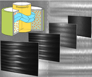
The evolution of the flow structure with varying control parameter  $\mathcal {R}$ was determined from flow visualization experiments. Flow maps, that is to say plots of the evolution of the flow structure with time or any time-dependent parameter, were constructed (using MATLAB) by selecting a four pixels wide band along the 360 pixels height of each image (see figure 1a) averaging along the 4 pixel (azimuthal) dimension to form an axial intensity profile, and stacking the profiles horizontally along the parameter evolution (see figure 2a and similar protocol in Lacassagne et al. (Reference Lacassagne, Cagney and Balabani2021)).

Figure 2. (a) Typical snapshot of the CCF, TVF and WVF regimes. (b) Space– $\mathcal {R}$ diagram for particle-free fluids RU experiment. The axial dimension is scaled by the gap size
  $\delta$ and vertical rectangles denote the
  $\mathcal {R}$ locations corresponding to the above snapshots. (c) Diagram of the Nusselt number
  $\mathcal {N}$ as a function of
  $\mathcal {R}$ for RU/RD experiments.
Frequency maps such as those reported in Dutcher & Muller (Reference Dutcher and Muller2009) and Lacassagne et al. (Reference Lacassagne, Cagney and Balabani2021) were also constructed for RU/RD experiments. For that purpose, sequences of 200 successive images were extracted for each shear-rate step during an acceleration/deceleration protocol, in the middle of the 30 s interval. This corresponded to 2.86 s at the frame rate of 70 f.p.s. or 1.43 s at 140 f.p.s. The fast Fourier transform of intensity signal as a function of time was then computed for each row of pixels (each axial location), and spectra were averaged axially in order to form a single frequency spectrum for the shear-rate step. Those spectra were then stacked vertically in order to form frequency maps, for which the  $x$-axis denotes time or any other time-dependent parameter such as
  $\mathcal {R}$, the
  $y$-axis is the frequency range, and the colour scale relates to the fast Fourier transform peak intensity representative of the energy content of each frequency. Frequency maps allowed us to identify unsteadiness in the flow, which appears in the form of discrete lines at characteristic frequencies. The critical conditions for the onset of unsteady flow states could thus be identified, and the temporal features of each flow state explored. This tool is used hereinafter in § 4.5.
3.1.4. Torque measurements
Torque measurements were performed during RU/RD protocols, simultaneously with visualization, by using the rheometer's torque sensor. Measurements were carried out by taking a time averaged torque value during each 30 s step at constant  $\dot {\gamma }$. The temperature was measured systematically before and after each experiment by a thermocouple (type K). It was found to remain within a
  ${\pm }0.5\,^{\circ }{\rm C}$ interval around the initial setpoint value of temperature, which is
  $20.8\,^{\circ }{\rm C}$.
The combination of flow visualization and torque measurements allowed us to analyse the torque evolution during in each flow structure and also to identify critical  $\mathcal {R}$ values for flow transitions (noted hereinafter
  $\mathcal {R}_c$). Indeed, the slope of the torque curves changes when the flow regime is modified, also corresponding to modifications in the flow map. Some of the reported transitions would not have been easily detectable using only one of the two indicators. A detailed example of critical Reynolds number detection is provided in Appendix A (see figure 12).
3.2. Suspension preparation and viscosity measurement
For the neutrally buoyant suspension, rigid spherical particles made of PMMA were used (GoodFellow, USA). Particles were first washed and sifted with cold water. Particles in the range  $40 \leqslant d_p \leqslant 63\ \mathrm {\mu } {\rm m}$ were kept, washed again with distilled water and finally dried at room temperature before use. The subsequent particle size distribution was measured by laser diffraction (LS Particle Size Analyzer, Beckman Coulter, USA), and their nominal mean diameter was
  $d_p \approx 50\ \mathrm {\mu } {\rm m}$.
The nominal gap-to-particle-size ratio was thus  $\delta /d_p = 30$. The density of particles was
  $1.19\ {\rm kg}\ {\rm m}^{-3}$. The particles were suspended in a density matched solvent composed of distilled water (
 $58.2\,\%$ by volume), glycerol (
 $41.8\,\%$ by volume) and sodium chloride, NaCl (144 ppt), with an equivalent density of
  $\rho = 1.1856 \simeq \rho _p\ {\rm kg}\ {\rm m}^{-3}$ at
  $21\,^{\circ }{\rm C}$. A small quantity of surfactant (less than
  $0.5\,\%$ by volume) Triton X-100 (Sigma Aldrich) was ultimately added to the suspension to avoid hydrophobicity of particles and adhesion or clustering at the air–water interface. Before the start of each test, the samples were put in an ultrasonic bath for
  $15$ minutes for resuspension, mixing and destruction of any particle agglomerates, and then in a vacuum for 30 minutes to remove any air bubbles that could have been entrapped in the viscous solvent.
The viscosity of the suspensions was measured using a plane–plane geometry mounted on the same rheometer (plate diameter 25 mm, gap of 1 mm). The viscosity increased with increasing particle volume fraction with a Krieger–Dougherty-like behaviour (see figure 1b) according to the correlation,  $\mu =\mu _{l}\left (1-\phi /\phi _{m}\right )^{-1.82}$. In the previous expression,
  $\phi _m = 0.55$ is the maximum packing concentration,
  $\mu _{l} = 0.0076\ {\rm Pa}\ {\rm s}$ is the viscosity of the suspending liquid mixture without particles.
3.3. Validation on a particle-free fluids
To validate the experimental protocol, preliminary experiments were performed for a Newtonian particle-free solution ( $\phi = 0$), in both RU/RD in the range of
  $17 < \mathcal {R}< 273$ and at a ramp rate of
  $\left | \Delta \mathcal {R} / \Delta \tau \right |= 0.0082$ (with the time scale
  $t_{d} \approx 0.351\ \mathrm {s}$).
Figure 2 shows a RU space– $\mathcal {R}$ diagram (space–time diagram where the time axis is replaced by
  $\mathcal {R}$, figure 2b), representative snapshots of flow structures encountered (figure 2a), and evolution of the effective Nusselt number as a function of the Reynolds number for these RU experiments, but also for the equivalent RD case. The expected flow structures and Nusselt behaviour are reported: purely azimuthal (CCF) at low
  $\mathcal {R}$ (flakes aligned in the azimuthal direction, no specific structure observed on the flow map); the gradual appearance of Ekman vortices at the bottom, in the form of lighter intensity patches, without any significant change in the Nusselt number figure 2(b) (Coles Reference Coles1965); primary bifurcation occurring here at
  $\mathcal {R}=150.8$ and leading to a stationary axisymmetric TVF illustrated by successive black and white stripes and by a sudden change of slope in the
  $\mathcal {N}$(
 $\mathcal {R}$) curve; a secondary bifurcation occurring at
  $\mathcal {R}=221$ with which Taylor vortices become unstable and undergo unsteady axial oscillations (WVF), also illustrated by a smooth change in slope for the
  $\mathcal {N}$–
 $\mathcal {R}$ curve. Our results for primary bifurcation critical
  $\mathcal {R}$ are close to theoretical analysis of Alibenyahia et al. (Reference Alibenyahia, Lemaitre, Nouar and Ait-Messaoudene2012) (
 $\eta = 0.914$
  $\varGamma \rightarrow + \infty$, primary bifurcation at
  $\mathcal {R}=151$) and experimental investigation of Dutcher & Muller (Reference Dutcher and Muller2009) (
 $\eta =0.912$,
  $\varGamma =60.7$, primary bifurcation at
  $\mathcal {R}=144 (\pm 4.2)$).
4. Results and discussion
4.1. Transitions and flow states
Torque measurements and visualization experiments have been performed for suspensions with concentrations  $\phi = 0\,\%, 1\,\%, 3\,\%, 6\,\%, 9\,\%, 12\,\%, 15\,\%, 20\,\%$. For the concentration of 28 %, only the primary bifurcation could be captured, due to the limitations in achievable angular velocities of the rheometer and considering the relatively high suspension viscosity (not reported in figure 1b but estimated from the Krieger–Dougherty fitting). In figure 3 the torque exerted by the solution on the inner cylinder is shown for all the suspensions. The solid lines and the dashed lines represent RU/RD experiments, respectively. The critical Reynolds number corresponding to the primary bifurcation is shown, as well as those for second and third bifurcations, in RU (square) and RD (circles). Note that all experiments have been repeated at least three times. Curves for single experiments are reported here, but average values for
  $\mathcal {R}_c$ will be provided later.

Figure 3. Variation of torque as a function of Reynolds for suspensions with concentration  $0\,\% \leq \phi \leq 20\,\%$.
Increasing particle concentration leads to the following effects. Firstly, a general increase in the torque applied to the inner cylinder is seen in the whole Reynolds range. This means that particles increase the power needed to rotate the inner cylinder at a given angular velocity. Secondly, a general increase in the slope of the torque versus  $\mathcal {R}$ is observed, which means that the torque increases faster with
  $\mathcal {R}$ when the concentration is increased. This is caused by the increased effective viscosity of the system which is related to particle–particle and particle–fluid interaction (see figure 1b). In all torque data, a sensible change in slope with the transition to TVF can be noted, as described earlier. With the transition of TVF–WVF, a less distinct change in slope is seen (symbolic slope shows for
  $\phi =20\,\%$ in figure 3). For suspensions at
  $\phi$ above 6 %, it can be noted that transition to TVF is more complex, and the change in slope less sharp: fluctuation is observed in torque measurements, and it will be shown thereafter to be due to the presence of non-axisymmetric flow patterns.
For a few experiments at selected concentration of  $\phi =3\,\%, 9\,\%, 15\,\%, 20\,\%$ the space–
 $\mathcal {R}$ and effective Nusselt number (
 $\mathcal {N}$) variation as a function of Reynolds number in RU/RD modes are shown along with the space–Reynolds diagram in RU mode in figure 4. In each figure, the critical Reynolds values corresponding to first, second and third bifurcation are marked by dashed lines, for RU tests. Identification of critical
  $\mathcal {R}_c$ is done by flow visualization and torque evaluation simultaneously in the manner described in § 3.2. A general decreasing trend for the first
  $\mathcal {R}_c$ is visible and will be discussed in detail in § 4.3. CCF, TVF and WVF can be described in a similar fashion than in the particle-free fluids case (see § 3.3). The previously mentioned non-axisymmetric state appears from suspension of 6 % (not shown here) and above, and is clearly visible in figure 4(b). It can be detected also in Nu–
 $\mathcal {R}$ plots (figure 3) from the more gradual and unclear changes in slope between CCF and TVF trends. The non-axisymmetric state (NAS) is evidenced by fluctuations in reflected light intensities occurring between CCF and the onset of TVF. Fluctuations here appear random when observed at the full experimental scale (full
  $\mathcal {R}$ range), however, when focusing on a narrower Reynolds range, a clear spiralling-like non-asymmetric structure can be observed (see figure 5). Further details about NAS will be given in § 4.2.

Figure 4. Space–Reynolds number diagram (RU) in addition to Nusselt–Reynolds evolution (RU/RD) showing the transitions from CCF to WVF for concentration of (a)  $\phi =3\,\%$; (b)
  $\phi =9\,\%$; (c)
  $\phi =15\,\%$; (d)
  $\phi =20\,\%$.

Figure 5. Close-up on the SVF regime: (a) snapshot photo of SVF flow from suspension of 15 %; (b) space time for a period of 806 s ( $\mathcal {R}$ between 140–145) taken by visualization in suspension of 15 %; (c) space time of 2 s (70 f.p.s.) taken from zooming in two different period of time in SVF flow in panel (b).
In the figure 4 flow maps, the effects of boundary conditions for lowest concentrations can be seen again in the form of Ekman vortices. As the concentration increases though this effect is reduced, and Taylor vortices are created just after the termination of non-axisymmetric flow, all at the same time. As pointed out by Benjamin (Reference Benjamin1978), in experimental investigations of TCF, CCF cannot satisfy the boundary conditions. Specifically, the bifurcation found in theoretical models with repeated period boundary conditions does not exist in experiments. However, it is obvious in the figure that the onset of Taylor cells is sharp even with an aspect ratio of 10. The origin of this sharpness has been explained by Cliffe, Mullin & Schaeffer (Reference Cliffe, Mullin and Schaeffer2012) and Mullin, Heise & Pfister (Reference Mullin, Heise and Pfister2017) as resulting from the breaking of an approximate symmetry between neighbouring states. In the case studied here, this would involve eight, 10 or 12 cells. It is interesting to note that almost all of the cases contain 10 cells with the exception of the 15 % (figure 4c) which contains eight cells. As mentioned before, the boundary conditions used in this experiment are slightly more complicated as the upper surface is free. However, the results appear to be in accord with the Cliffe et al. (Reference Cliffe, Mullin and Schaeffer2012) interpretation.
In parallel, in the figure 4 Nusselt plots, the primary bifurcation is captured in a clear way, either by a sharp (when transitioning to TVF) or smooth (when a non-axisymmetric state is involved) change of the Nusselt slope, regardless of the presence or absence of Ekman vortices. This additionally suggests that Ekman vortices and the boundary conditions do not significantly affect the effective friction forces exerted on the inner cylinder and thus the Nusselt values. Hence, Nusselt value fluctuations evidenced at higher particle concentrations cannot be ascribed to boundary effects in CCF. The inflection point related to TVF–WVF transition is still subtle, as it was in the  $\mathcal {T}$–
 $\mathcal {R}$ plots.
The Nusselt number related to CCF ( $\mathcal {R} < \mathcal {R}_{c_1}$) is almost constant and is around one. Rheologically speaking, this means that torque depends linearly on viscosity and viscosity does not depend on the shear rate variation. This linear behaviour is observed by Dash et al. (Reference Dash, Anantharaman and Poelma2020) (
 $\mathcal {N}$ with respect to
  $Ta$) for the concentration of less than 25 %, and Kang & Mirbod (Reference Kang and Mirbod2021) in their numerical results. On the other hand
  $\mathcal {N} \sim \mathcal {R}^{c}$ with an exponent
  $c$ that depends on concentration has been observed by Ramesh et al. (Reference Ramesh, Bharadwaj and Alam2019). They reported an increasing in effective Nusselt number with increasing
  $\mathcal {R}$ and proposed dimensionless torque
  $G \sim \dot {\gamma }\left (r=r_{i}\right ) / \mu (\phi ) \sim \mathcal {R}^{\alpha }$ with
  $\alpha =1$ for a particle-free fluids and
  $\alpha >1$ for a suspension with
  $\phi \geqslant 0.05$ in the CCF regime. Finally, Dash et al. (Reference Dash, Anantharaman and Poelma2020) also observed an increase of
  $\mathcal {N}$ with
  $Ta$ (Taylor number, alternative of
  $\mathcal {R}$), but for concentrations over 25 %. They argued that this could be due to anisotropy in the microstructure of non-colloidal suspension flow, and non-homogeneous distribution of particle concentration in the radial direction which comes from the migration of particles, and modifies the local shear rate and viscosity along the gap. In this study, particle concentrations remain below 25 % with the exception of one test case, and the particle size to gap size ratio is below the one used in Dash et al. (Reference Dash, Anantharaman and Poelma2020). Hence, microstructure anisotropy is not expected, which is consistent with the torque scaling observations in CCF. Torque scaling in TVF and VWF will be further discussed in § 4.6.
4.2. Non-axisymmetric states
A specific feature of the flow of particle suspensions for volume fractions at  $\phi >6\,\%$ is the existence of non-axisymmetric flow states. A snapshot of non-axisymmetric state for suspension of 15 % in RU protocol is shown in figure 5(a). Non-axisymmetric states were generally evidenced in Dash et al. (Reference Dash, Anantharaman, Greidanus and Poelma2019), Ramesh et al. (Reference Ramesh, Bharadwaj and Alam2019) and Majji et al. (Reference Majji, Banerjee and Morris2018) experimentally and in the numerical study of Kang & Mirbod (Reference Kang and Mirbod2021). The flow structure present here is a SVF regime such as the one reported by Majji & Morris (Reference Majji and Morris2018) and Ramesh et al. (Reference Ramesh, Bharadwaj and Alam2019). This regime consisted of axially travelling vortex pairs. Figure 5(b) shows a space–time diagram for a 806 s time span, corresponding to a
  $\mathcal {R}$ range of 140–145, recorded at 70 f.p.s. In the middle of this space–time plot, a change of travelling direction occurs. Similar changes in direction were observed in all experiments for concentrations of 6 % and above, seemingly randomly with no particular pattern in time or space. Figure 5(c) illustrates this behaviour by displaying close-ups of figure 5(b) on 2 s time spans before and after this changing direction.
The effect of SVF on  $\mathcal {N}$ can be seen in figure 4 in the form of a slope drop in Nusselt values resulting in a smoother change of slope for CCF to TVF transition, through intermediate scaling. While Ramesh et al. (Reference Ramesh, Bharadwaj and Alam2019) did not report any changes in the Nusselt scaling associated with SVF, Kang & Mirbod (Reference Kang and Mirbod2021) noticed a slight drop in Nusselt number for SVF and WSVF at a concentration of
  $10\,\%$ with spherical particle size of
  $\delta /d_p=30$. We here report a first experimental observation of how SVF is associated with
  $\mathcal {N}$ scaling variations.
Figure 6 shows evolution of Nusselt number normalized by Nusselt value at which the non-axisymmetric state starts (for each concentration separately) as a function of dimensionless  $\mathcal {R}$ (
 $(\mathcal {R}-\mathcal {R}_{c_{(SVF)}})/(\mathcal {R}_{c_{(T V F)}}-\mathcal {R}_{c_{(SVF)}})$). In this way, every plot in the Nusselt axis starts from 1 and in the Reynolds axis the values remain between 0–1. This helps when comparing the evolution of Nusselt number with
  $\mathcal {R}$ within the SVF range.

Figure 6. Evolution of Nusselt number normalized by critical Nusselt number of SVF state for each concentration as a function of dimensionless Reynolds number in the SVF period for  $\phi =6\,\%, 9\,\%, 12\,\%, 15\,\%, 20\,\%$. Solid and dashed lines represent the RU and RD protocol, respectively.
The first visible feature is that the  $\mathcal {N}$ trend goes from mildly increasing
  $\mathcal {R}$ at
  $\phi =6\,\%$ to non-monotonic and globally constant or decreasing at higher
  $\phi$. In other words, the presence of particles (
 $\phi >6\,\%$), which cause SVF, also has a non-trivial effect on the Nusselt number and can reduce the torque (or the increase of torque with
  $\mathcal {R}$) applied to the inner cylinder.
A proposed explanation for this non-monotonic behaviour is the following. The presence of particles promotes axially travelling non-axisymmetric flow structures and causes a delay of the transition from unsteady (SVF) to stationary (TVF) instability. During this phenomenon, convective momentum transfer decays (as mentioned by Kang & Mirbod (Reference Kang and Mirbod2021)), resulting in a reduction of the torque exerted on the inner cylinder. Simultaneously, increasing the rotational velocity leads to an increase in kinetic energy, which ultimately overcomes the energy loss induced by the presence of particles. The Reynolds number at which this shift occurs corresponds to a local minimum of Nusselt number.
On the other hand, Kang & Mirbod (Reference Kang and Mirbod2021) showed that in an SVF state, particle migration induced by shear leads to the accumulation of particles inside the core of one of the two vortices of a counter-rotating pair (and not both of them) resulting in an heterogeneous particle distribution. This non-homogeneity is intensified by increasing Reynolds number and concentration. We believe that the latter also may cause the reduction and variation of Nusselt number as can be seen in figure 6.
4.3. Onset of primary and secondary instabilities
Let us now consider the global picture and report the critical Reynolds number values for transition to the various flow states encountered. The average  $\mathcal {R}_c$ related to all bifurcations and for all concentrations are listed in table 1, and represented in figure 7(a). These values are obtained from the average on three times repetition for each concentration, and the uncertainty (error bars on the figure) is estimated as the standard deviation of
  $\mathcal {R}_c$ on the three tests. For concentrations less than 6 %, no SVF is encountered before TVF, and so there are only two bifurcations, the primary bifurcation being from CCF to TVF. For concentrations above 6 %, the primary bifurcation is CCF–SVF, the secondary bifurcation is SVF–TVF, and the tertiary bifurcation is TVF–WVF. For the concentration of 28 %, as mentioned before, just the primary instability is captured and shown.

Figure 7. (a) Variation of critical Reynolds  $\mathcal {R}_c$ corresponding to primary (square symbol), secondary (circle symbol) and tertiary (triangle symbol) bifurcation as a function of concentration. Values have been averaged over three experiments and the standard deviation serves as error bars. The solid line represent RU and the dashed line represents RD test. (b) Critical Reynolds number correspond to the primary instability (TVF or SVF), normalized by the critical Reynolds number for
  $\phi =0\,\%$, as a function of concentration. Comparison with experimental data of Ramesh et al. (Reference Ramesh, Bharadwaj and Alam2019), Majji & Morris (Reference Majji and Morris2018) and theoretical data of Gillissen & Wilson (Reference Gillissen and Wilson2019), Ali et al. (Reference Ali, Mitra, Schwille and Lueptow2002) is provided. Solid lines represent RU and dashed line represent RD protocol. (c,d) difference between
  $\mathcal {R}_c$ at the onset and
  $\mathcal {R}_c$ at the end of (c) SVF (
 $\phi \geqslant 6\,\%$ only) and (d) TVF in RU (full squares) and RD (full circles), and data from the literature. Error bars are cumulative uncertainties derived from each
  $\mathcal {R}_c$ detection.
Table 1. Summary of critical Reynolds numbers corresponding to primary, secondary and tertiary bifurcation and their standard deviation ( $\pm$ intervals) for the suspension with concentration
  $0\,\% \leq \phi \leq 28\,\%$. Due to the significant increase in viscosity of the solution for the concentration of 28 % and shear rate limitations of the rheometer, higher-order instabilities could not be attained for this fluid and the test was limited to the detection of the primary bifurcation. These data values are represented in figure 7.

Several observations can be made from figure 7(a).
(i) There is a clear trend for a decrease in the critical
 $\mathcal {R}$ for the primary bifurcation with increasing particle concentration (the primary bifurcation being either CCF–TVF or CCF–SVF), and thus for a destabilization of CCF.
(ii) The critical
$\mathcal {R}$ for transition to WVF is globally constant for $\phi <15\,\%$ and sharply decreases for the higher concentration measured.(iii) A weakly hysteretic behaviour appears for primary bifurcations from
$\phi >12\,\%$, with a difference between $\mathcal {R}_c$ of RU/RD. For secondary and tertiary bifurcations, it can be observed even sooner, for $\phi >3\,\%$.


For the secondary and tertiary bifurcations,  $\mathcal {R}_c^{(down)}$
  $< \mathcal {R}_c^{(up)}$ at all concentrations above
  $3\,\%$, corresponding to subcritical bifurcations. This is consistent with the results of Ramesh et al. (Reference Ramesh, Bharadwaj and Alam2019) and Dash et al. (Reference Dash, Anantharaman and Poelma2020) (
 $\phi = 0.10, 0.20$), who reported subcritical behaviours and degrees of subcriticality (
 $\mathcal {R}_{c}^{(up)}-\mathcal {R}_{c}^{(down)}$) increasing with increasing
  $\phi$. The hysteretic behaviour is not trivial as far as the primary bifurcation is concerned: no hysteresis is observed for
  $\phi <3\,\%$ where this bifurcation involves the CCF–TVF transition, and no hysteresis is observed for
  $3\,\%<\phi \leq 9\,\%$ where it involves the CCF–SVF transition. For
  $9\,\%<\phi \leq 20\,\%$,
  $\mathcal {R}_c^{(up)} > \mathcal {R}_c^{(down)}$. The trend is reversed in the
  $\phi =28\,\%$ case where the primary bifurcation CCF–SVF also becomes subcritical (
 $\mathcal {R}_c^{(down)} < \mathcal {R}_c^{(up)}$). About apparent hysteresis effects of the onset of time-dependence in TCF, it was shown by Pfister & Gerdts (Reference Pfister and Gerdts1981) that there is ‘critical slowing down’ of the dynamics at the onset of wavy motion. Hence, ramping through the Hopf bifurcation point would have to be carried out extremely slowly to avoid apparent up and down parameter shifts in the estimates of the bifurcation point. Fortunately, these effects usually occur over small ranges of
  $\mathcal {R}$ but could well explain this small apparent hysteresis for TVF–WVF transition. Nevertheless, for both possibilities (apparent hysteresis or real hysteresis) it is still related to the presence of the particles, as for
  $\phi >3\,\%$ we can see this hysteresis.
Focusing on the effect of particles on the CCF stability, figure 7(b) shows the  $\mathcal {R}_c / \mathcal {R}_{c,0}$ for the primary bifurcation as a function of concentration and comparison with data from different studies in the literature, both experimental or theoretical. In particular, the first black solid line represents the theoretical result of Gillissen & Wilson (Reference Gillissen and Wilson2019) (with geometrical parameters identical to the experiments of Majji et al. (Reference Majji, Banerjee and Morris2018)). In this study, the stability was estimated based on a suspension stress theory which ignores all non-hydrodynamic forces but accounts for fluid–particles interactions in non-dilute suspensions. An added extra stress is induced by the lubrication forces between the spheres, but no direct contact (collision) between them is considered. The theory also assumes no density difference between particle and fluid (fluid and particle inertia are the same on a volumetric basis, and hydrodynamic force are negligible). The results of Gillissen & Wilson (Reference Gillissen and Wilson2019) qualitatively agree with the theoretical result of Ali et al. (Reference Ali, Mitra, Schwille and Lueptow2002) (black dashed line in figure 7), based on a two-fluids theory that ignores interactions between spheres and is subsequently restricted to
  $\phi <5\,\%$, in the sense that particles globally lead to a destabilization of CCF with increasing particle concentration. The trend and asymptotic behaviour at
  $\phi =0\,\%$ are yet quite different from each other. Experimental results of Ramesh et al. (Reference Ramesh, Bharadwaj and Alam2019), with control parameter of
  $\varGamma =11$,
  $\eta =0.914$ close to the present study but with a difference in boundary condition (lid on top) and particle size ratio,
  $d_p/\delta = 37.5$, seem to follow the theory of Ali et al. (Reference Ali, Mitra, Schwille and Lueptow2002) in an almost straight line. An interesting agreement between their results and the present study is that in the moderate concentration, the difference between
  $\mathcal {R}_c^{up}$ and
  $\mathcal {R}_c^{down}$ grows (
 $\mathcal {R}_c^{down}-\mathcal {R}_c^{up}>0$). The results of Majji et al. (Reference Majji, Banerjee and Morris2018) are comprised between the trends of the two theories and also follow linear variations.
The results of the present study are also well framed by the two theories, yet closer to the trend of Gillissen & Wilson (Reference Gillissen and Wilson2019), especially in the low particle volume fraction where the forces (non-hydrodynamic) acting on the particles are modelled more accurately. This agreement underlines the importance of hydrodynamic particle–particle interactions and particle induced fluid stress, even at relatively low particle volume fractions. The limitation when comparing our results with the theory of Gillissen & Wilson (Reference Gillissen and Wilson2019) is that they assumed that primary instability modes were necessarily axisymmetry, while the primary instability modes for  $\phi >3\,\%$ are here non-axisymmetric.
4.4. $\mathcal {R}$ range for flow state existence

Beyond the estimation of critical  $\mathcal {R}$ values, interesting information can be obtained by measuring the span of Reynolds number spent in each flow state:
  $\mathcal {R}_{c_{{TVF}}} - \mathcal {R}_{c_{{SVF}}}$ for SVF and
  $\mathcal {R}_{c_{{WVF}}} - \mathcal {R}_{c_{{TVF}}}$ for TVF. Figure 7(c) shows the evolution of this quantity for (a) SVF and (b) TVF, in accordance with the results reported in figure 7(a,b).
The range of  $\mathcal {R}$ corresponding to SVF firstly increases until a 15 % concentration is reached, and then reduces, in both RU/RD cases. In other words, there is an optimum concentration value for which the existence of SVF is maximized, regardless of the hysteretic behaviour of bifurcations, and the implications of this result in terms of torque and potential for mixing will be discussed later. Studies of Dash et al. (Reference Dash, Anantharaman and Poelma2020), Ramesh et al. (Reference Ramesh, Bharadwaj and Alam2019) and Majji et al. (Reference Majji, Banerjee and Morris2018), on the other hand, did not report this non-monotonic behaviour.
The range of TVF existence, unlike that of SVF, simply decreases with increasing concentration. This decrease is all the more pronounced as the concentration exceeds 15 %, in accordance with the sharp decrease in the critical  $\mathcal {R}$ for the onset of WVF reported in this range in figure 7(a). This trend is in good qualitative agreement with those of Majji et al. (Reference Majji, Banerjee and Morris2018) (
 $\phi <20\,\%$) and Dash et al. (Reference Dash, Anantharaman and Poelma2020). The difference in magnitude is due to the variations in aspect ratio (larger for Majji et al. (Reference Majji, Banerjee and Morris2018) and even larger for Dash et al. (Reference Dash, Anantharaman and Poelma2020)), smaller aspect ratios that lead to a damping of the waviness of the Taylor vortex, a delaying of the onset of WVF, and thus an increased span for TVF. Note that Ramesh et al. (Reference Ramesh, Bharadwaj and Alam2019) report values similar to those of this study for a very similar aspect ratio, but yet found a concentration-independent behaviour for TVF (
 $\phi <25\,\%$).
4.5. Frequency map
In order to describe the unsteady features of some flow states (SVF, WVF), we here present frequency maps of RU/RD experiments for selected  $\phi =0\,\%, 9\,\%, 15\,\%, 20\,\%$ values, in figure 8. Frequency maps at other
  $\phi$ were also produced, but not shown here for the sake of brevity.

Figure 8. Frequency maps in RU (a,c,e,g) and RD (b,d,f,h) protocols at  $\phi =0\,\%$ (a,b),
  $\phi =9\,\%$ (c,d),
  $\phi =15\,\%$ (e,f) and
  $\phi =20\,\%$ (g,h). Horizontal axis limits are set on the same Reynolds interval for better comparison, which leads to empty regions as concentration (and viscosity) increase and limit the Reynolds range that can be explored. Note that
  $\phi =20\,\%$; the recording frequency was 140 f.p.s., corresponding to a maximum detectable frequency of 70 Hz, versus 35 Hz for the other cases where the recording frequency was 70 f.p.s. The vertical axis has been scaled accordingly.
Characteristic frequencies can be captured as long as they are below the Nyquist criterion ( $f< 1/2 \times f_{acq}$ where
  $f_{acq}$ is acquisition frequency), here equal to 35 Hz for the first three cases and 70 Hz for
  $\phi =20\,\%$. All frequency maps share a common feature: the presence of a clear line with a frequency linearly increasing with
  $\mathcal {R}$, that can be observed for example between
  $f=5$ Hz at
  $\mathcal {R}=150$ and
  $f=10$ Hz at
  $\mathcal {R}=250$ in the
  $\phi =0$ case. It can be shown that the characteristic frequency of those lines simply scale as
  $f=f_{\varOmega } / 2{\rm \pi}$ where
  $f_{\varOmega }$ is an inner cylinder rotation frequency. This line thus corresponds to the ability of the method to detect the rigid body rotation frequency of the inner cylinder, which varies linearly with
  $\varOmega$ and thus with
  $\mathcal {R}$. Harmonics
  $f_k=k \times f_{\varOmega } / 2{\rm \pi}$ can also be identified in some cases (Dutcher & Muller Reference Dutcher and Muller2009; Cagney & Balabani Reference Cagney and Balabani2019).
Now, CCF and TVF being steady laminar states, they are not expected to display any spectral signature other than the line associated with the rotation speed of the inner cylinder and its harmonics. This can be verified for example in figure 8  $\phi =0\,\%$ (RU/RD), where CCF and TVF are essentially indistinguishable for the frequency map alone.
In the SVF state ( $\phi >6\,\%)$ a clear line appears at a frequency lower than
  $f_{\varOmega }$ during its lifetime, along with higher-order harmonics (additional fainter lines seen above), as seen in figure 8 for
  $\phi =9\,\%-20\,\%$. This frequency simply scales as the vortex travelling velocity divided by the spatial wavelength. In other words, the intensity signal probed at a given altitude fluctuates as vortices travel axially. The SVF lines disappear when the flow enters the TVF regime, thus allowing this transition to be evidenced on the frequency maps as well as on the flow maps reported previously. Interestingly, the frequency of SVF was always
  $f_{{SVF}}\approx 0.5 f_{\varOmega }$.
The onset of WVF finally corresponds to the appearance of one or several distinct additional lines, the frequency of which are not harmonics of  $f_{\varOmega }$. For the particle-free fluids case (
 $\phi =0\,\%$, see figure 8), the main wavy frequency at the onset of WVF is such that
  $f_{{WVF}}>f_{\varOmega }$ , consistent with Cagney & Balabani (Reference Cagney and Balabani2019) and Lacassagne et al. (Reference Lacassagne, Cagney and Balabani2021), and more specifically
  $f_{{WVF}}/f_{\varOmega }=2.83$ close to the value of 2.5 reported by Coles (Reference Coles1965).
However, unlike what was observed in Cagney & Balabani (Reference Cagney and Balabani2019) and Lacassagne et al. (Reference Lacassagne, Cagney and Balabani2021),  $f_{{WVF}}$ decreases with increasing
  $\mathcal {R}$, unlike
  $f_{\varOmega }$. This discrepancy is believed to be due to the slight difference in upper boundary condition (free surface here versus rigid lid in Cagney & Balabani (Reference Cagney and Balabani2019) and Lacassagne et al. (Reference Lacassagne, Cagney and Balabani2021)). Note that while Majji et al. (Reference Majji, Banerjee and Morris2018) did not produce frequency maps, the flow maps reported in their figure 5 suggest that they would also have observed a decrease in
  $f_{{WVF}}$ with similar boundary conditions, as in this work.
It can be noted that the dynamic frequency behaviour of flow regime is an analogue in RU/RD protocols (see figure 8), not only for  $0\,\%$ but also for the suspension cases reported hereinafter. When the volume fraction is increased, the first effect observed is that of a decrease in the
  $f_{{{WVF}}}$ (see figure 8,
  $\phi = 0\,\%-15\,\%$). The decreasing behaviour is retrieved for the
  $20\,\%$ case, with a dramatic increase of
  $f_{{WVF}}$ (see figure 8,
  $\phi =20\,\%$). Unlike the WVF state,
  $f_{{SVF}} \simeq 0.5 f_{\varOmega }$ for all the concentration. On the other hand, the modulation of WVF by particle concentration with increasing Reynolds number (
 $\text {slope}_{f_{{WVF}}}/\text {slope}_{f_{\varOmega }}$) seems independent of particle concentration. Dash et al. (Reference Dash, Anantharaman and Poelma2020) previously reported values of
  $f_{{WVF}}/f_{\varOmega }$ at the onset of WVF between 3.5–3.9 for particle concentration between 3.4 % and 30 %, with yet a higher aspect ratio and lower gap to particle ratio. However, the wavy frequency for their particle-free case was not presented. Thus, the question of whether the origin of this difference is the aspect ratio, the gap-to-particle ratio, or combination of factors remains open.
The dynamics of SVF and WVF can be further described by comparing two indicators: the value of the dominant characteristic frequency at the onset of SVF and WVF (at the critical  $\mathcal {R}_c$), here scaled by the
  $f_{\varOmega }$ at this same onset and written
  $f_{{SVF}}/f_{\varOmega }$ and
  $f_{{WVF}}/f_{\varOmega }$; and the ratio of the frequency slope of the SVF and WVF main line to the frequency slope of the inner cylinder. This is done for all
  $\phi$ values (included those illustrated in figure 8). The two indicators are reported in figure 9(a,b) (in absolute value), respectively. Note that the first indicator is also illustrated by empty circles plotted at the onset where the frequency is probed, in figure 8. In figure 9(a), arrows also indicate the trend for the evolution of the wavy frequency after the onset (increasing for upward pointing arrow, decreasing for downward pointing arrows). The RU/RD protocols are shown with square/circle symbols, respectively.

Figure 9. (a) Dominant characteristic frequency of wavy vortices at the onset of the WVF state normalized by the inner cylinder frequency ( $f_{{WVF}}/f_{\varOmega }$), plotted as a function of concentration. The up and down arrows illustrate the increasing or decreasing trend of this wavy frequency with increasing
  $\mathcal {R}$ after the onset. (b) Absolute values of the ratio between the slope of the dominant wavy frequency with
  $\mathcal {R}$, and the slope of
  $f_{\varOmega }$. The
  $+$ (negative, respectively) symbols indicate that the ratio was positive (negative, respectively), i.e. that the frequency of the inner cylinder and WVF state have gradients of the same sign (opposite, respectively) along
  $\mathcal {R}$. Square and circle symbols in both (a,b) plots represent RU/RD protocols, respectively (note that the value of
  $f_{{WVF}}/f_{\varOmega }$for
  $\phi =12\,\%$ in left-hand figure is equal to 0.02).
Starting with the first indicator (frequency at the onset), a first observation is the fact that the trend for the evolution of  $f_{{WVF}}$ with increasing
  $\mathcal {R}$ is a decreasing one for all concentrations except for
  $\phi =12\,\%$ and
  $15\,\%$. Suspension behaviour, in the WVF state, can be divided into three parts according to this indicator. In the first part for
  $\phi \leqslant 9\,\%$, the frequency is globally higher than the frequency of the inner cylinder (above the horizontal dashed line equal to 1 in figure 9a) and experiences a decreasing trend.
At  $\phi =$
  $9\,\%$, the frequency of the wavy state is approximately equal to the frequency of the inner cylinder, and a further increase in particle concentration leads to entering a second part where
  $f_{{WVF}} < f_{\varOmega }$ at the onset of the wavy state and the wavy frequency evolution trend reverses to become increasing with
  $\mathcal {R}$. The minimum onset frequency is found at
  $\phi =12\,\%$. The third part is for 15 % and above, where there is an abrupt increase in frequency but again the trend is declining. The third part, here illustrated by the single
  $\phi =20\,\%$ data point, corresponds to a dramatic increase in
  $f_{{WVF}}/ f_{\varOmega }$ and a return to a decreasing trend.
Figure 9(b) brings additional information on those trends, thanks to the second indicator which relates to the intensity of the decrease/increase of the WVF state frequency relative to the inner cylinder frequency ( $\text {slope}_{f_{{WVF}}}/\text {slope}_{f_{\varOmega }}$). This indicator is reported in absolute values in order to better compare the magnitudes, but
  $+$ or
  $-$ signs indicate whether the ratio was increasing (stemming from an increasing wavy frequency) or decreasing (when the wavy frequency decreased with
  $\mathcal {R}$ in the previous figure). The most striking result is that the magnitude of this indicator remains roughly constant with concentration, regardless of the sign of the slopes, values varying between 4.2–5.6, i.e. on a
  $\pm 15\,\%$ interval around the average 4.9 value. For the SVF, this indicator is
  ${\approx }0.5$ for all concentrations.
It is finally worth noting that there is almost no difference in the RU/RD process for the two indicators, except for the slope ratio at  $\phi =20\,\%$, indicating that the dynamics of WVF at and after the onset is independent of the potentially hysteretic nature of the bifurcation allowed to trigger it. The fact that increasing the concentration (and so increasing effective viscosity) first leads to a decrease of the frequency ratio at the onset of the WVF state (until
  $\phi =12\,\%$) seems consistent with the rise in effective viscosity. Yet after that, in the intermediate concentration range, the expected trend is reversed. It is believed that this non-trivial behaviour marks the appearance of significant interactions between particles, overcoming hydrodynamic forces. Further increasing particle concentration up to
  $\phi =20\,\%$, particle–particle interactions are expected to become dominant.
4.6. $\mathcal {N}$ versus $Ta$ scaling


In the previous sections, we have described the succession of flow states and their dynamic behaviour using flow visualization coupled with torque measurements in order to accurately detect flow transitions. In this section and the following, we will use only torque measurements to discuss the friction dynamic behaviour associated with each flow state. Figure 10 shows consolidated (average from three tests) plot of Nusselt number variation as a function of Taylor number for the inner cylinder for all suspensions in RU/RD experiments (some of the curves were previously reported in figure 4 for  $\mathcal {N}$ as a function of
  $\mathcal {R}$). The solid lines and the dashed lines represent RU/RD experiments, respectively. Here the Taylor number is used rather than
  $\mathcal {R}$ in order to compare our scaling exponents with those reported in the literature. It should be noted that
  $Ta$ can be expressed as a function of
  $\mathcal {R}$ and of geometrical parameters, as described in § 1, so for a given geometry, both control parameters can equally be used.

Figure 10. (a) Consolidated plots (averaged on all repeats at identical  $\phi$) for the Nusselt number as a function of the Taylor number. Panel (b) reports the evolution of
  $\alpha$ and (c)
  $\beta$ coefficients with
  $\phi$ where
  $\mathcal {N}\sim Ta^{\alpha }$ and
  $\mathcal {N}\sim Ta^{\beta }$ are power law scalings in TVF and WVF, respectively. Full lines and squares, and dashed lines and circles, illustrate RU/RD experiments, respectively. Insets in panel (a) show plots of
  $\mathcal {N} \times Ta^{-\alpha }$ (left-hand inset) and
  $\mathcal {N} \times Ta^{-\beta }$ (right-hand inset) as a function of Reynolds number, justifying the power law fittings in TVF (left-hand inset) and WVF (right-hand inset), respectively. The vertical dashes denote the TVF range and onset of WVF in the left-hand and right-hand insets, respectively.
For each curve, the TVF and WVF domains are then extracted and fitted by functions of the type  $\mathcal {N}\sim Ta^p$, with
  $p=\alpha$ for TVF and
  $p=\beta$ for WVF. Values of the
  $\alpha$ and
  $\beta$ exponents are then represented as a function of
  $\phi$ in the two upper left-hand-corner insets. This allows us to compare the slopes of
  $\mathcal {N}$–Ta plots for selected flow states at all particle concentrations. In the
  $\phi =0\,\%$ case,
  $\alpha \simeq 0.6$, and
  $\beta \simeq 0.3$, with no obvious difference between RU/RD protocols. As
  $\phi$ increases up to
  $15\,\%$, the
  $\alpha$ slope for Nusselt number versus Reynolds number in the TVF state gradually decreases, down to a value of 0.49 in RU, and a sensible difference between RU/RD exponents appears. Then it is reversed after 15 %, with 0.53 for
  $\phi =20\,\%$. A similar decay with increased
  $\phi$ is observed for the
  $\beta$ exponent, this time until the
  $\phi =12\,\%$ concentration is reached 0.18. The trend is then reversed with a further increase in
  $\beta$ for
  $\phi =15\,\%$ and
  $20\,\%$. For higher
  $Ta$ values still in the WVF regime, attained by RU experiments, and with
  $\eta = 0.917$ and
  $\varGamma = 21.7$, Dash et al. (Reference Dash, Anantharaman and Poelma2020) reported that a
  $\mathcal {N}(\mu _{l})\sim Ta^{0.23}$ scaling (Nusselt number based on the solvent viscosity
  $\mu _l$, which is not expected to change the scaling exponent). Ramesh et al. (Reference Ramesh, Bharadwaj and Alam2019) in their figure 27, on the other hand, report a
  $\mathcal {N} \sim Ta^{0.26}$ scaling for
  $\phi =10\,\%$ RD experiments and
  $\mathcal {N} \sim Ta^{0.35}$ for
  $\phi =20\,\%$. Our results thus agree well with the range observed in the literature.
The presence of suspended particles at concentrations below  $\phi =15\,\%$ in the TVF state apparently reduces the transverse momentum transfer (and so there is added energy dissipation in the system). This behaviour is reversed at higher concentrations. It is believed that part of the explanation can be found in the existence of the shear induced migration of particles which comes from non-homogeneous microstructure between them in suspension and this may result in enhancing the transverse momentum transfer in the system and so on torque (in other words drag reduction). Likely the reason for this early slope change in the
  $\phi =12\,\%$ WVF state may be because of increasing interaction between particles, while the suspension is well mixed in this flow regime, so this enhancing in transverse momentum transfer begins earlier.
4.7. Friction coefficient
The above results can be completed by showing another parameter quantifying the torque exerted on the inner cylinder, namely the friction factor. It is a dimensionless measure of the torque that the fluid exerts on the inner rotating cylinder and is computed as the ratio of the wall shear stress to the dynamic pressure. This parameter relates quite well to a common requirement in practical applications, the need to quantify the power required to overcome the frictional drag of a rotating shaft. The friction coefficient for a rotating cylinder can be defined as follows (Kang & Mirbod Reference Kang and Mirbod2021):
 \begin{equation} C_{M_{z}}=\frac{\mathcal{\tau}}{\rho {\rm \pi}r_{i}^{2} h (r_{i} \varOmega_{i})^{2} / 2}. \end{equation}
This can be expressed as is such that
 \begin{equation} G=f(\eta)\times C_{M_z} \times \mathcal{R}^2 \end{equation}
with the suspension Reynolds number ( $\mathcal {R}= \rho \left (r_{i} \varOmega _{i} \right ) \delta / \mu _s =$
  $\rho \dot {\gamma } \delta ^{2} / \mu _s$). Thus
 \begin{equation} \mathcal{N} = G / G_{lam} \simeq g (\eta) \times C_{M_z} \times \mathcal{R}. \end{equation}
 So  $C_{M_z}$ is the coefficient of proportionality between
  $\mathcal {N}$ and
  $\mathcal {R}$. It is in some way related to the slope of
  $\mathcal {N} = f(Ta)$ curves since for these we write
 \begin{equation} \mathcal{N} \sim Ta^\alpha. \end{equation}
 Figure 11 shows the evolution of friction coefficient for  $\phi =0\,\%$ and
  $15\,\%$. In the
  $\phi =0\,\%$ case, CCF, TVF and WVF are identified by black, blue and red lines, respectively. In the
  $\phi =15\,\%$ case the additional SVF state is shown in purple. Friction coefficients corresponding to RU/RD experiments are plotted in solid and dashed lines, respectively.

Figure 11. Evolution of friction coefficient for  $\phi =0\,\%$ and
  $15\,\%$. In the
  $\phi =0\,\%$, CCF, TVF and WVF are identified by black, blue and red lines, respectively. In the
  $\phi =15\,\%$ the additional SVF state is shown in purple. Friction coefficients corresponding to RU/RD experiments are plotted in solid and dashed lines, respectively.
In the  $\phi =0\,\%$ case, the friction coefficient decreases quickly in CCF, down to the point at which the primary instability occurs in the system (
 $\mathcal {R}=150.8$ in RU and
  $\mathcal {R}=148$ in RD). This point is the local minimum value in terms of the friction coefficient. Afterwards, further increase in
  $\mathcal {R}$ leads to the development of counter-rotation vortices characteristic of TVF states, and the friction coefficient increases until a local maximum value is reached, just before the secondary bifurcation to WVF occurs (
 $\mathcal {R}=200$ in RU and
  $\mathcal {R}=148$ in RD). The friction coefficient then decreases again with increasing
  $\mathcal {R}$ in the WVF state. So, TVF thus corresponds to a state where the friction coefficient is maximized, and low values of
  $C_{M_z}$ are encountered for high
  $\mathcal {R}$ or locally just before the onset of TVF.
In the  $\phi =15\,\%$ case, the CCF behaviour is similar to the one for
  $\phi =0\,\%$. When entering the SVF state (purple line,
  $\mathcal {R}=132$ in RU and
  $\mathcal {R}=138$ in RD), the decreasing
  $C_{M_z}$ decays even more rapidly with
  $\mathcal {R}$, allowing the friction coefficient to reach lower values than those encountered for
  $\phi =0\,\%$. A local minimum of
  $C_{M_z}$ is reached, this time not at the transition between CCF and TVF, but in the middle of the SVF regime. This minimum is preserved until the transition to the TVF state occurs right after this point at
  $\mathcal {R}=163$ in RU mode (and
  $\mathcal {R}=161$ in RD mode), and the friction coefficient increases again with increasing
  $\mathcal {R}$, moderately this time. When the WVF state is reached,
  $C_{M_z}$ begins to decrease, with a slope similar to the one observed for
  $\phi =0\,\%$.
The general behaviour of the friction coefficient with  $\mathcal {R}$ in CCF, TVF and WVF is thus comparable in the two cases, but an additional interesting behaviour is introduced by SVF. Kang & Mirbod (Reference Kang and Mirbod2021) also reported in their numerical study that spiral patterns caused by the presence of particles tend to reduce the friction coefficient on the inner cylinder for the suspension of 10 %. The axial travelling of SVF reduces the convective momentum transfer in the radial direction; in consequence, it results in the reduction of the Nusselt number and torque acting on the inner cylinder.
Summarizing §§ 4.6 and 4.7, the effect of particle concentration on  $\alpha$ and
  $\beta$ coefficients suggests that transverse momentum transfer is enhanced at concentrations above 15 % in the TVF state, and at concentrations above 12 % in the WVF state. On the another hand, in the semidilute suspension (concentrations below 12 %) there is (i) a significantly reduced friction coefficient in SVF and WVF states; and (ii) a weaker increase of friction coefficient in TVF state compared with particle-free solutions. This is an interesting input in terms of power consumption efficiency. Note that the Nusselt number and friction coefficient are related together: a reduction in transverse momentum transfer means a lower friction coefficient.
4.8. hydrodynamic concentration subregimes
Typically in the particle-suspension literature (Ancey & Vollm Reference Ancey and Vollm2005; Morris Reference Morris2009), particle suspensions are said to be in the dilute regime for  $\phi <5\,\%$, semidilute regime for
  $5\,\%\leq \phi \leq 30\,\%$ and concentrated regime for
  $\phi >30\,\%$. According to this nomenclature, all of the particle suspensions used here belong to the dilute and semidilute regimes. It is worth noting that this classification was built on cases without inertia, at vanishing
  $\mathcal {R}$. The various parameters identified in this work allow us to identify three distinct concentration subregimes (separated by two critical concentrations), in which the hydrodynamic behaviours are quite different, and that we will thus label as ‘hydrodynamic concentration subregimes’ (HCR).
(i) The first concentration regime (HCR1) is found for
$\phi <6\,\%$, and is included in the conventional dilute regime. It corresponds to a hydrodynamic behaviour very similar to the $\phi =0\,\%$ with only a minor increase in torque corresponding to the minor increase in suspension apparent viscosity: Nusselt scalings with $Ta$ are similar, unlike what was observed in Majji et al. (Reference Majji, Banerjee and Morris2018), there is no evident decrease in critical Reynolds numbers for the onset of primary and secondary instability, and subsequently no change in parameter range for flow states existence, or in the nature of such bifurcations. Transitions do not appear hysteretic. Only the frequency map analysis allows us to detect an effect of particles on unsteady flow dynamics: the wavy frequency at the onset of WVF decreases with increasing particle concentration, indicating that the presence of particles even at very low concentrations plays a role in the selection of the most unstable mode responsible for the development of WVF.(ii) The second regime (HCR2) corresponds to the
$6\,\%\leq \phi <15\,\%$ range and is also included in what would be called the dilute regime when looking only at the particle concentration value. However, from a hydrodynamic point of view, it is very different from the previous one (HCR1). The torque exerted on the inner cylinder significantly increases in magnitude owing to the increases suspension viscosity, but more importantly, a new unsteady non-axisymmetric flow state appears between CCF and TVF, SVF modifying the nature of the primary instability and a sensible decrease in its critical Reynolds number, in good qualitative agreement with the theory of Gillissen & Wilson (Reference Gillissen and Wilson2019). The $\mathcal {R}$ range of SVF increases with yet no particular effects on the $\mathcal {R}$ range of TVF, and hence on the onset of WVF. Yet, the higher-order transitions (SVF–TVF or TVF–WVF) become notably subcritical. Particle concentration also has an influence on the dynamics in the WVF regime, indeed both the frequency at the onset and the Nusselt scaling exponent vary non-monotonically with a local minimum around $12\,\%$ or $15\,\%$. The Nusselt scaling exponent in TVF also decreases in this HCR2 range. All of this results in a minimum friction coefficient found at $\phi =15\,\%$ in the middle on the SVF $\mathcal {R}$ range, and indicates a complex interplay between particles and fluid flows.(iii) The last regime (HCR3) corresponds to the
$\phi >15\,\%$ cases investigated here and would thus be equivalent to the ‘semidilute’ concentration regime. In that regime, there is a dramatic increase of viscosity and thus of the torques exerted on the inner cylinder, but also in Nusselt scaling exponent for TVF and WVF state. The $\mathcal {R}$ ranges of SVF and TVF are reduced in accordance with the global destabilization of all intermediate flow regimes (SVF, TVF). The frequency of the mode responsible for the onset of WVF is also greatly increased.


It is believed that the origin of this behaviour, and thus the nature of bifurcation, comes from the competition between particle–fluid and particle–particle interaction, the latter becoming gradually dominant over the former as the concentration of regime is changing.
5. Summary and conclusions
In this study, in-depth investigation of the behaviour of the TCF of non-colloidal neutrally buoyant suspensions of particles in ( $\phi \in 0\,\%-20\,\%$) a Newtonian fluid (
 ${\rm water}+{\rm glycerol}$) was conducted, with a focus on the nature of bifurcations, unsteady dynamics and torque scaling. The major findings can be summarized as follows.
(i) The addition of particles intuitively leads to an increase in the torque magnitude exerted on the inner cylinder at equivalent Reynolds number, and of its increase rate (see figure 3). In the presence of particles, the required power to rotate the inner cylinder increases. The amount of this increase is small for concentrations up to
$\phi =6\,\%$, significant for $\phi =6$ to 15 % and sharp for $\phi =20\,\%$. This is expected from the Krieger–Dougherty-like increase in the suspension's apparent viscosity.(ii) For
$\phi <6\,\%$ the transition was CCF–TVF–WVF. From $\phi \geq 6\,\%$, an additional non-axisymmetric state called SVF was observed leading to a CCF–SVF–TVF–WVF transition for both RU/RD protocols.(iii) Increasing particle concentration up to
$\phi =15\,\%$, a non-monotonic effect of SVF was observed on the Nusselt number (see figure 6) and the $\mathcal {R}$ range of SVF increased.(iv) The critical Reynolds number for the primary instability decreases with increasing particle concentration above
$3\,\%$, with the nature of primary instability changing from TVF to SVF for $\phi >6$. For $\phi >15\,\%$, a strong destabilization of CCF and TVF is found. The primary instability is found to be alternatively subcritical/supercritical but the secondary (TVF) and tertiary (WVF) bifurcations are always subcritical (figure 7). Our results for the onset of the primary instability critical Reynolds qualitatively agree with the theory of Gillissen & Wilson (Reference Gillissen and Wilson2019) (see figure 7b) that account for particle induced stresses in the flow.(v) An optimum of the
$\mathcal {R}$ range of existence can be found for SVF at $\phi =15\,\%$ but not for TVF.(vi) Frequency analysis suggests that the presence of particles plays a role in the most unstable mode leading to onset of WVF. On the other hand, the modulation of SVF and WVF by particles with increasing Reynolds number (
$\text {Slope}_{f_{{WVF}}}/\text {Slope}_{f_{\varOmega }}$ and $\text {Slope}_{f_{{SVF}}}/\text {Slope}_{f_{\varOmega }}$) seems independent of particle concentration in the range presently investigated.(vii) In the TVF state, an increase of particle concentration up to
$\phi =15\,\%$ leads to a $\mathcal {N}$ slope decrease, while after $\phi =15\,\%$ the $\mathcal {N}$ slope increases again. Conversely, in the WVF state, the $\mathcal {N}$ slope has quasi-constant value up to $\phi =6\,\%$, a reduction in the $\mathcal {N}$ slope is observed for $\phi = 6\,\%-12\,\%$, and an increase for $\phi >12\,\%$(viii) The friction coefficient allowed us to evidence the existence of a minimum friction coefficient in SVF.
(ix) Three HCR were reported based on the various hydrodynamic characteristic of the suspension.


Even though the available data on TCF of non-colloidal particle suspensions has been recently enriched by several comprehensive studies including this one, there is still a lack of systematic investigation of the effects of geometrical parameters (radius ratio, curvature ratio, aspect ratio or particle-size-to-gap ratio) on the flow dynamics indicator presented here (which we performed on a single geometry). In the long term, introducing outer cylinder rotation would offer interesting perspectives, in that non-axisymmetric states that are observed here as a primary instabilities in non-Brownian suspensions, were explored before in the case of counter-rotating cylinders (Coles Reference Coles1965).
As a perspective, the existence of an unsteady non-asymmetric state at moderate Reynolds number shows promising potential for mixing applications: unlike CCF and TVF, SVF is associated with axial velocities and fluid particles are able to travel axially in time at yet lower  $\mathcal {R}$ values compared with WVF, and thus lower friction. Moreover, as previously mentioned, an optimal friction coefficient can be found in this SVF regime. So, SVF could thus be seen as a promising way to enhance mixing with moderate power consumption in semidilute particle suspension. This could be an asset for the design of cooling devices employing non-colloidal smart fluids. Changes in dynamic properties (torque, Nusselt number, friction coefficient) are also expected to be closely related to changes in flow microstructure or at least spatially variable suspension properties. Therefore, a focus of future works could be to investigate experimentally the effects of possible inhomogeneity in particle concentration distribution during the SVF state, from low to high concentrations.
Funding
Financial support from Region Hauts de France and Institut Mines Télécom is gratefully acknowledged.
Declaration of interests
The authors declare no conflict of interest.
Appendix A. Methodology for finding $\mathcal {R}_c$

For each experiment (RU or RD), a figure similar to figure 12 is produced. It comprises two curves (blue and orange). The orange one shows the Reynolds value changing and the blue one shows the dimensionless torque. Both of theme are as a function of time. The slope change in torque is detected and by tracing a vertical line the corresponding critical  $\mathcal {R}_c$ is found. This value is then verified by visual inspection of the recorded video at the specified time. For cases where a transition to unsteady state is detected (SVF, WVF), the inspection of frequency maps and identification of the onset of additional frequencies ultimately validates the critical
  $\mathcal {R}_c$ detection.

Figure 12. (a) Space–time diagram of a RU experiment prepared from 2627 frames (photograph captured in interval of 4.3 s) during 11250 s for a Newtonian fluid without particles. The axial dimension is scaled by the gap size  $\delta$. Here
  $\mathcal {R}$ varied between 17 and 273 from left to right, with
  $\varDelta \mathcal {R} / \varDelta \tau = 0.0082$. (b) Measured dimensionless torque as a function of time (left-hand axis in blue) and corresponding Reynolds number (right-hand vertical axis, orange curve).
Appendix B. Geometric characteristics of the works compared in this article as well as their observed flow transitions
Table 2. Comparison of geometrical parameters in related experimental and theoretical studies and present study for non-Brownian suspensions flow in TC geometry with rotating inner cylinder. Also, flow transition order related to different concentrations for doing experimental study. The letters C, N, T and W in the abbreviation of CTW, CNTW, CNTNW, CNW and CN represents CCF, NAS, TVF and WVF, respectively. Here NAS represents all the SVF, RIB and coexisting states ( ${\rm TVF}+{\rm SVF}$, TVF, WVF, etc.).


