2. Problem setup

We study the two-dimensional flow past a transversely oscillating cylinder in a finite-width channel. The cylinder is prescribed to oscillate with period $T$ and amplitude $A$ for a specified inflow velocity $U$. Instead of the period, we consider the wavelength $\lambda =UT$ as an equivalent parameter. Figure 2 shows a sketch of the setup. We non-dimensionalise the velocity field $\boldsymbol {u}$ by rescaling with $U$. All lengths, including the amplitude $A$ and the wavelength $\lambda$, are non-dimensionalised on the diameter of the cylinder, $D$. The pressure $p$ is scaled on the associated viscous scale, $\mu U/D$, where $\mu$ is the dynamic viscosity of the fluid, and time is scaled on the advective timescale, $D/U$. The flow (in the moving frame of reference) is then governed by the non-dimensional Navier–Stokes equations

(2.1a,b)\begin{equation} Re\left(\frac{\partial \boldsymbol{u}}{\partial t} + (\boldsymbol{u} \boldsymbol{\cdot} \boldsymbol{\nabla})\boldsymbol{u}\right) ={-} \boldsymbol{\nabla} p +\nabla^2 \boldsymbol{u} \quad \text{and} \quad \boldsymbol{\nabla} \boldsymbol{\cdot} \boldsymbol{u}=0, \end{equation}

where the Reynolds number is $Re=\rho UD/\mu$, with $\rho$ being the density of the fluid. In the moving frame of reference we use a Cartesian coordinate system, in which the centre of the cylinder is located at

(2.2a,b)\begin{equation} x_{cyl}(t)=0, \quad y_{cyl}(t)=A \sin(2{\rm \pi} t/\lambda). \end{equation}

On the surface of the moving cylinder we impose the no-slip condition

(2.3a,b)\begin{equation} u=0, \quad v = \frac{{\rm d} y_{cyl}}{{\rm d} t} = (2{\rm \pi} A /\lambda) \cos (2{\rm \pi} t/\lambda). \end{equation}

We also impose the boundary conditions

(2.4)\begin{equation} u=1, \quad v=0, \quad \text{at } x={-}L_{inlet} \text{ and at } y={\pm} H/2, \end{equation}

corresponding to a uniform inflow and a no-slip condition relative to the moving channel walls. Furthermore we allow the outlet to remain (pseudo-)traction free, i.e.

(2.5)\begin{equation} \begin{pmatrix} -p +\partial u/\partial x\\ \partial v/\partial x \end{pmatrix}=\begin{pmatrix} 0\\ 0 \end{pmatrix} \quad \text{at } x=L_{outlet}. \end{equation}

Figure 2. Sketch of the problem setup and the boundary conditions, all expressed in non-dimensional variables. The setup is described by a Cartesian coordinate system where the origin coincides with the centre of the cylinder at $t=0$.

In the main computational part of this study we fix the Reynolds number to be 100, well within the regime of two-dimensional flow for a stationary cylinder (Barkley & Henderson Reference Barkley and Henderson1996). Furthermore, oscillations of the cylinder stabilise the two-dimensional flow (Gioria et al. Reference Gioria, Jabardo, Carmo and Meneghini2009), as also found experimentally by Griffin (Reference Griffin1971). We have chosen to use a value of $Re=100$ so that we can directly compare our results with those by Matharu et al. (Reference Matharu, Hazel and Heil2021) and Leontini et al. (Reference Leontini, Stewart, Thompson and Hourigan2006).

Our aim is to find time-periodic solutions of (2.1a,b)–(2.5). For a given solution $\boldsymbol {u}(x,y,t;A,\lambda )$ the corresponding vorticity field can be computed as

(2.6)\begin{equation} \omega(x,y,t;A,\lambda)=\boldsymbol{\nabla} \times \boldsymbol{u}(x,y,t;A,\lambda). \end{equation}

To investigate topological bifurcations in the vorticity field, simulations have been performed at four different values of the wavelength: $\lambda =5.5$, $6.085$, $6.5$ and $6.7$. The value $\lambda _{St}=6.085$ is obtained from the relationship

(2.7)\begin{equation} T/T_{St}=\lambda_{St} St =1, \end{equation}

where $T$ is the period of the imposed cylinder oscillations and $T_{St}$ is the period at which vortices are shed in the same flow past a stationary cylinder, i.e. the Strouhal period. The Reynolds number of $Re=100$ corresponds to the Strouhal number $St=0.16434$ when using the Reynolds–Strouhal number relationship given by Williamson (Reference Williamson1988). The results for $\lambda =\lambda _{St}$ can be compared directly with the studies by Matharu et al. (Reference Matharu, Hazel and Heil2021). Having selected the values of the two free parameters, $Re$ and $\lambda$, we consider time as the bifurcation parameter and monitor the cusp bifurcations in the vorticity field during a complete oscillation and repeat this as the amplitude is varied.

3. Numerical method

We performed numerical simulations using the open-source finite-element library oomph-lib (Heil & Hazel Reference Heil and Hazel2006). The Navier–Stokes equations were spatially discretised with quadrilateral Taylor–Hood elements, within which the velocities and the pressure are represented by quadratic and piecewise linear polynomials, respectively. For the time-integration of the problem we employ the second-order accurate BDF2 scheme with 320 time steps per period of the imposed oscillations. The simulations were performed on a computational domain with dimensions $H=20$, $L_{inlet}=10$ and $L_{outlet}=70$. The mesh was built from a coarse base mesh and uniformly refined five times. The base mesh is shown with thicker lines in figure 3. In the square central box the nodal positions in the mesh are updated every time step according to the imposed cylinder oscillations. The annular region with unit radius surrounding the cylinder hole is made rigid so that no compression occurs in this part of the mesh as the cylinder oscillates. To reduce the computational cost some of our simulations were performed on a mesh where only the central downstream region and the square central box (highlighted in figure 3 with a red box) were uniformly refined five times whereas the remainder was refined only three times. Upon comparison of mesh types we find no qualitative difference in the vorticity topology.

Figure 3. Illustration of the computational domain. The thick black lines show the base mesh and the thin black lines show the mesh after four uniform refinements. In the actual simulations the mesh was uniformly refined five times in the central region (marked with a red box) and three times outside this region.

The simulations are initiated by computing the steady solution for a fixed cylinder at $Re=0$. We use this result as an initial condition to compute the solution for a slightly higher Reynolds number and continue in this manner until we reach $Re=100$. This solution is used as an initial condition for the oscillating cylinder simulations where the amplitude of the oscillations is gradually increased in the first two periods. The time-periodicity of the solution is assessed by computing the $L^2$-norm of the change in the velocity components over one period of the cylinder oscillation. We deem the solution to be time-periodic when the relative change in the $L^2$-norm of the velocity components drops below $10^{-6}$. We have chosen this threshold value by comparing with simulations where the relative change has instead dropped below $10^{-8}$. In the cases examined, we observe no topological difference between the two associated vorticity fields, at least not to the level of precision at which we keep track of the cusp bifurcation points.

To compute the vorticity field and its derivatives we first need the derivatives of the velocity field. However, the solution computed via our simulations is only required to be continuous between elements, therefore the derivatives between elements can be discontinuous. To compute smooth approximations of the required derivatives we use the patch-based flux-recovery technique implemented in oomph-lib, which is based on an implementation of the Z2 error estimator (Zienkiewicz & Zhu Reference Zienkiewicz and Zhu1992). For a validation of the method in connection with topological bifurcations see Appendix A of Heil et al. (Reference Heil, Rosso, Hazel and Brøns2017). The extrema (and saddle points) are located at the intersections of the nullclines $\partial _x \omega =0$ and $\partial _y \omega =0$.

4. An extended classification of wakes with topological variations downstream

When characterising a wake pattern, it is common to use the terminology introduced by Williamson & Roshko (Reference Williamson and Roshko1988). The classification method assumes that the entire wake can be classified as a single type of pattern. Hence, it is implicitly assumed that, once formed, all vortices are translated downstream without any change in the topology. In this section, we argue that a more detailed classification is necessary to be able to describe the wake structure accurately and also to understand the topological changes in the transition from 2S to $\text {P}+ \text {S}$.

Figure 4 contains snapshots of two different vorticity fields. The vorticity fields have been computed for a cylinder oscillating with the same wavelength but different amplitudes. The feature points for vortices, i.e. the vorticity extrema, are marked with black dots. For $A=0.80$, we see that two single vortices are shed in each oscillation cycle, and this structure is preserved when the vortices are advected downstream. Therefore, we classify the wake pattern as a full 2S wake. For a larger amplitude of $A=1.110$ we see a $\text {P}+ \text {S}$ wake pattern that is advected downstream with no topological change. In these examples the terminology introduced by Williamson & Roshko (Reference Williamson and Roshko1988) is fully sufficient for classifying the wake pattern. However, this is not always the case. Figure 5 shows four snapshots of the vorticity field for $A=1.085$, a value between the cases in figure 4. From the number of vorticity extrema we observe that two pairs of vortices (black dots) are shed during one oscillation cycle, producing a vortex shedding pattern that looks like a 2P mode in the near wake. In each vortex pair one of the vortices is much weaker than the other, and quickly disappears. The black curves in figure 5 encircle a set of vortices shed during an oscillation cycle. In the first snapshot, the encircled region highlights two pairs of vortices. Figure 5(b) shows the vorticity field in the last time step before one of the highlighted vortices disappears via a cusp bifurcation with a saddle point. Exactly half a period later, a second cusp bifurcation occurs, and the set of highlighted vortices then consists of two single vortices. The snapshot in figure 5(b) shows the last time step before the second cusp bifurcation occurs. Despite the fact that we observe topological bifurcations as the vortices move downstream, the spatio-temporal $Z_2$ symmetry is preserved throughout the process. Therefore, we conclude that these topological bifurcations are not associated with a loss of symmetry. In order to describe the topological variations of the vorticity field downstream, we introduce an extended classification where we keep track of the pattern of vortices that are created in one cycle, and indicate with a superscript $n\in \mathbb {N}$ how long the pattern persists. If the pattern exists for more than $n-1$ periods but less than $n$ periods, we designate the superscript $n$. In the example in figure 5(b), the vortices that originate from the same cycle are grouped together with dashed and dotted lines. A dashed line indicates that the group consists of two pairs of vortices, whereas a dotted line indicates that the group consists of two single vortices. We observe that three groups with a 2P pattern are present in the vorticity field just before the first of the two weaker vortices disappears. Hence, we conclude that the vortices in a 2P group move downstream for between two and three periods before any topological bifurcation occur. The wake in figure 5 therefore has a $(2\text {P})^3(2\text {S})^\infty$ vortex pattern. Here $\infty$ denotes that no further bifurcations are observed in the entire computational domain. In addition, we do not address the changes in the wake structure that occur far downstream. It is well-known that the primary vortex street breaks down into a nearly parallel shear flow with a Gaussian profile at a certain downstream distance, before a secondary vortex street of larger scale may appear further downstream (Karasudani & Funakoshi Reference Karasudani and Funakoshi1994). Note, that in the extended classification, the standard 2S and $\text {P}+ \text {S}$ wakes are denoted $(2\text {S})^\infty$ and $(\text {P}+ \text {S})^\infty$, respectively.

Figure 4. Snapshots of the vorticity field computed at $Re=100$ for $\lambda =6.085$ and (a) $A=0.80$ and (b) $A=1.110$. All extrema of vorticity are marked with black dots. The black curves encircle a set of vortices that are shed in a single oscillation cycle. Only part of the computational domain is shown.

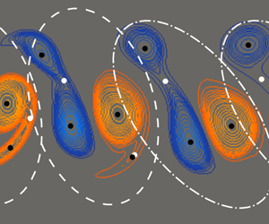
Figure 5. Four snapshots of a vorticity field computed at $Re=100$ for $\lambda =6.085$ and $A=1.085$. The times shown indicate when the snapshots were taken during a single cylinder oscillation with a normalised period of one. All extrema of vorticity are marked with black dots and saddle points are marked with white dots. The black curves highlight how the vortices that are shed in one oscillation cycle move downstream during a period of oscillation. The vortices that originate from the same cycle are grouped together in (b). A dashed line indicates that the group consists of two pairs of vortices, whereas a dotted line indicates that the group consists of two single vortices.

Figure 6 shows a snapshot of a vorticity field computed for an oscillating cylinder with $\lambda =6.7$ and $A=1.140$. This vorticity field is an example of another wake pattern with topological variations downstream. The snapshot is taken at the last time step before the weaker vortex in the lower pair disappears in a cusp bifurcation. Since this is the only topological bifurcation that occurs, the wake is classified as mode $(2\text {P})^2(\text {P}+ \text {S})^\infty$. One could argue that the wake patterns in figures 5 and 6 are really just 2S and $\text {P}+ \text {S}$ modes, and the extra vortices that our classification detect in the shear layers have no significant impact. However, as we show in § 5, it is precisely these vortices that become important when describing the topological development from a 2S to a $\text {P}+ \text {S}$ wake.

Figure 6. A snapshot of a vorticity field computed at $Re=100$ for $\lambda =6.7$ and $A=1.140$. All extrema of vorticity are marked with black dots and saddle points are marked with white dots. The snapshot is taken at the last time step before a cusp bifurcation occurs. The vortices that originate from the same cycle are grouped together. A dashed line indicates that the group consists of two pairs of vortices, whereas a dash-dotted line indicates that the group consists of a pair and a single vortex.

5. Topological bifurcations of the vorticity field at the symmetry-breaking pitchfork bifurcation point

As mentioned in the introduction, a very recent paper by Matharu et al. (Reference Matharu, Hazel and Heil2021) showed that the symmetry breaking that occurs in the transition from 2S to $\text {P}+ \text {S}$ mode at $Re=100$ is due to a dynamical bifurcation, namely a subcritical pitchfork bifurcation. The vorticity field of the 2S wake pattern preserves the spatio-temporal symmetry condition

(5.1)\begin{equation} \omega(x,y,t)={-}\omega(x,-y,t+1/2). \end{equation}

Matharu et al. (Reference Matharu, Hazel and Heil2021) analysed simulations with increasing amplitude values and construct a bifurcation diagram by measuring the magnitude of the symmetry breaking in the computed solutions. For the vorticity field, the magnitude of the symmetry breaking is given by the norm of the difference between $\omega (x,y,t)$ and $-\omega (x,-y,t+1/2)$, i.e.

(5.2)\begin{equation} \varepsilon=\tfrac{1}{2}\|\omega(x,y,t)+\omega(x,-y,t+1/2)\|. \end{equation}

A sketch of their bifurcation diagram is shown in figure 7. At $A = A_2$, a subcritical pitchfork bifurcation occurs, creating two branches of asymmetric time-periodic solutions $\omega ^+$, $\omega ^-$. Each of these branches subsequently gain stability via fold bifurcations at $A=A_1$. The stable branch associated with $\varepsilon =0$ corresponds to time-periodic solutions for which the vorticity field satisfies the symmetry condition (5.1), e.g. the 2S wake pattern shown in figure 4(a). On the two outer branches of the pitchfork the symmetry condition is broken, meaning that $\varepsilon \neq 0$. The vorticity field of a solution on the positive branch $\omega ^+$ has a conjugate solution on the negative branch $\omega ^-$ satisfying

(5.3)\begin{equation} \omega^+(x,y,t)={-}\omega^-(x,-y,t+1/2). \end{equation}

Figure 7. A sketch of the bifurcation diagram illustrating the subcritical pitchfork bifurcation at $A=A_2$ and secondary fold bifurcations at $A=A_1$. In the specific case where the cylinder oscillates with $\lambda = 6.085$, Matharu et al. (Reference Matharu, Hazel and Heil2021) determined the bifurcation parameter values to be $A_1\approx 1.0680$ and $A_2\approx 1.0855$.

We distinguish the bifurcating branches by parameterising $\omega ^+$ by $\varepsilon$, and $\omega ^-$ by $-\varepsilon$. The $\text {P}+ \text {S}$ wake pattern shown in figure 4(b) is an example of a wake pattern on the stable part of the $\omega ^-$ branch, which corresponds to the branch of solutions for which the vortex pair sheds below the centreline. In the conjugate time-periodic solution, which lies on the $\omega ^+$ branch, the pair of vortices are instead shed above the centreline. The history of the cylinder motion determines which of the two conjugate solutions a simulation converges to. By reversing the initial motion of the cylinder, we obtain the solution belonging to the opposite branch in the bifurcation diagram. These conjugate solutions correspond to two solutions that satisfy (5.3) on the outer (stable) branches of the pitchfork. As the pitchfork is subcritical, three stable periodic solutions exist for amplitudes in the range $A_1\leq A \leq A_2$, however, the solutions on the branches $\omega ^+$ and $\omega ^-$ are related through the relationship in (5.3) and are identical from a topological point of view; hence we refer to the region as ‘bistable’ in the following.

In this section, we analyse the topological bifurcations of the vorticity field that occur as a direct result of the dynamical bifurcation. As a starting point for the analysis, we introduce a parameter $\sigma$ moving along the outer branches in the bifurcation diagram as illustrated in figure 8(a). For the sake of simplicity we let $\sigma = 0$ correspond to the symmetric vorticity field located at the pitchfork bifurcation point. As the two outer branches correspond to the two conjugate solutions it follows that

(5.4)\begin{equation} \omega(x,y,t,\sigma)={-}\omega(x,-y,t+1/2,-\sigma). \end{equation}

We start by considering a non-degenerate critical point in the vorticity field for $\sigma =0$, i.e. a point $(x^*,y^*,t^*)$ satisfying

(5.5)\begin{equation} \left.\begin{array}{c@{}} \partial_x\omega(x^*,y^*,t^*,0)=0,\\ \partial_y\omega(x^*,y^*,t^*,0)=0,\\ |{\boldsymbol{\mathsf{H}}}^\omega(x^*,y^*,t^*,0)|\neq 0. \end{array}\right\} \end{equation}

The implicit function theorem ensures that the critical point is preserved for sufficiently small values of $|\sigma |$. Furthermore, the continuity of ${\boldsymbol{\mathsf{H}}}^\omega$ guarantees that $|{\boldsymbol{\mathsf{H}}}^\omega |$ will not change sign, which means that a critical point identified as a vortex will persist. In the case where all critical points in the symmetric vorticity field are non-degenerate, the vortices persist when the symmetry is broken and no topological bifurcations occur as a direct result of the dynamical bifurcation.

Figure 8. (a) A bifurcation diagram illustrating the subcritical pitchfork bifurcation. The branches of stable and unstable solutions are represented by thick lines and dashed lines, respectively. (b) The bifurcation diagram in a neighbourhood of $(x,\sigma )=(x^*,0)$. Two different cusp bifurcation curves are parameterised by $\hat {X}$ and $\tilde {X}$.

If, on the other hand, the symmetric vorticity field at $\sigma =0$ has topological variations downstream, then there exists a cusp bifurcation point $(x^*,y^*,t^*)$ satisfying

(5.6)\begin{equation} \left.\begin{array}{c@{}} \partial_x\omega(x^*,y^*,t^*,0)=0,\\ \partial_y\omega(x^*,y^*,t^*,0)=0,\\ |{\boldsymbol{\mathsf{H}}}^\omega(x^*,y^*,t^*,0)|=0,\\ \text{tr}({\boldsymbol{\mathsf{H}}}^\omega(x^*,y^*,t^*,0))\neq 0. \end{array}\right\} \end{equation}

To characterise the topological changes that occur at $\sigma =0$ we need to assume some regularity at the cusp bifurcation point $(x^*,y^*,t^*)$. Consider the following Jacobian

(5.7)\begin{equation} {\boldsymbol{\mathsf{J}}}_*= \left.\begin{pmatrix} \partial_{xx}\omega & \partial_{xy}\omega & \partial_{xt}\omega\\\partial_{xy}\omega & \partial_{yy}\omega & \partial_{yt}\omega\\ \partial_x|{\boldsymbol{\mathsf{H}}}^\omega| & \partial_y|{\boldsymbol{\mathsf{H}}}^\omega| & \partial_t|{\boldsymbol{\mathsf{H}}}^\omega| \end{pmatrix}\right|_{(x^*,y^*,t^*,0)}. \end{equation}

If the determinant of ${\boldsymbol{\mathsf{J}}}_*$ is non-zero, i.e.

(5.8)\begin{equation} \left.\left(-\left| \begin{pmatrix} \partial_{xx}\omega & \partial_{xy}\omega\\\partial_x|{\boldsymbol{\mathsf{H}}}^\omega| & \partial_y|{\boldsymbol{\mathsf{H}}}^\omega| \end{pmatrix}\right|\partial_{yt}\omega+\left| \begin{pmatrix} \partial_{xy}\omega & \partial_{yy}\omega\\\partial_x|{\boldsymbol{\mathsf{H}}}^\omega| & \partial_y|{\boldsymbol{\mathsf{H}}}^\omega| \end{pmatrix}\right|\partial_{xt}\omega\right)\right|_{(x^*,y^*,t^*,0)}\neq 0, \end{equation}

it follows from the implicit function theorem that there exist unique local functions $x=\hat {X}(\sigma )$, $y=\hat {Y}(\sigma )$, $t=\hat {T}(\sigma )$ satisfying

(5.9a–c)\begin{equation} \hat{X}(0)=x^*,\quad \hat{Y}(0)=y^*,\quad \hat{T}(0)=t^*, \end{equation}

and

(5.10)\begin{equation} \left.\begin{array}{c@{}} \partial_x \omega(\hat{X}(\sigma),\hat{Y}(\sigma),\hat{T}(\sigma),\sigma)=0,\\ \partial_y \omega(\hat{X}(\sigma),\hat{Y}(\sigma),\hat{T}(\sigma),\sigma)=0,\\ |{\boldsymbol{\mathsf{H}}}^\omega(\hat{X}(\sigma),\hat{Y}(\sigma),\hat{T}(\sigma),\sigma)|=0. \end{array}\right\} \end{equation}

The functions $\hat {X}$, $\hat {Y}$ and $\hat {T}$ provide a parametric representation of a curve of topological cusp bifurcations. The shape of the bifurcation curve is given by the derivatives of $\hat {X}$, $\hat {Y}$ and $\hat {T}$ at the bifurcation point $\sigma =0$. By implicit differentiating the equations in (5.10) we obtain the following system of equations,

(5.11)\begin{equation} {\boldsymbol{\mathsf{J}}}_*\begin{pmatrix} \hat{X}'(0)\\ \hat{Y}'(0)\\ \hat{T}'(0) \end{pmatrix}=\begin{pmatrix} \partial_{x\sigma}\omega(x^*,y^*,t^*,0)\\ \partial_{y\sigma}\omega(x^*,y^*,t^*,0)\\ \partial_{\sigma}|{\boldsymbol{\mathsf{H}}}^\omega(x^*,y^*,t^*,0)| \end{pmatrix}. \end{equation}

As ${\boldsymbol{\mathsf{J}}}_*$ is non-singular the explicit expressions of $\hat {X}'(0)$, $\hat {Y}'(0)$ and $\hat {T}'(0)$ are well-defined as a combination of the elements in the Jacobian and the right-hand side of (5.11). Rather than computing the explicit expressions, we consider a second bifurcation point that is a necessary result of the symmetry for $\sigma =0$. From the condition in (5.4) it follows that

(5.12)\begin{equation} \left.\begin{array}{c@{}} \partial_x\omega(x^*,-y^*,t^*+1/2,0)={-}\partial_x\omega(x^*,y^*,t^*,0)=0,\\ \partial_y\omega(x^*,-y^*,t^*+1/2,0)=\partial_y\omega(x^*,y^*,t^*,0)=0,\\ |{\boldsymbol{\mathsf{H}}}^\omega(x^*,-y^*,t^*+1/2,0)|=|{\boldsymbol{\mathsf{H}}}^\omega(x^*,y^*,t^*,0)|=0, \\ \text{tr}({\boldsymbol{\mathsf{H}}}^\omega(x^*,-y^*,t^*+1/2,0)) ={-}\text{tr}({\boldsymbol{\mathsf{H}}}^\omega(x^*,y^*,t^*,0))\neq0, \end{array}\right\} \end{equation}

and

(5.13)\begin{align} &\left.\left(-\left| \begin{pmatrix} \partial_{xx}\omega & \partial_{xy}\omega\\ \partial_x|{\boldsymbol{\mathsf{H}}}^\omega| & \partial_y|{\boldsymbol{\mathsf{H}}}^\omega| \end{pmatrix}\right|\partial_{yt}\omega+\left| \begin{pmatrix} \partial_{xy}\omega & \partial_{yy}\omega\\ \partial_x|{\boldsymbol{\mathsf{H}}}^\omega| & \partial_y|{\boldsymbol{\mathsf{H}}}^\omega| \end{pmatrix}\right|\partial_{xt}\omega\right) \right|_{(x^*,-y^*,t^*+1/2,0)}\nonumber\\ &\quad =\left.\left(-\left| \begin{pmatrix} -\partial_{xx}\omega & \partial_{xy}\omega\\ \partial_x|{\boldsymbol{\mathsf{H}}}^\omega| & -\partial_y|{\boldsymbol{\mathsf{H}}}^\omega| \end{pmatrix}\right|\partial_{yt}\omega+\left| \begin{pmatrix} \partial_{xy}\omega & -\partial_{yy}\omega\\ \partial_x|{\boldsymbol{\mathsf{H}}}^\omega| & -\partial_y|{\boldsymbol{\mathsf{H}}}^\omega| \end{pmatrix}\right|(-\partial_{xt}\omega)\right) \right|_{(x^*,y^*,t^*,0)}\nonumber\\ &\quad =\left.\left(-\left| \begin{pmatrix} \partial_{xx}\omega & \partial_{xy}\omega\\ \partial_x|{\boldsymbol{\mathsf{H}}}^\omega| & \partial_y|{\boldsymbol{\mathsf{H}}}^\omega| \end{pmatrix}\right|\partial_{yt}\omega+\left| \begin{pmatrix} \partial_{xy}\omega & \partial_{yy}\omega\\ \partial_x|{\boldsymbol{\mathsf{H}}}^\omega| & \partial_y|{\boldsymbol{\mathsf{H}}}^\omega| \end{pmatrix}\right|\partial_{xt}\omega\right)\right|_{(x^*,y^*,t^*,0)}\neq 0. \end{align}

As expected, we can therefore conclude that $(x^*,-y^*,t^*+1/2)$ is a cusp bifurcation point satisfying all the same conditions as $(x^*,y^*,t^*)$. By a similar argument, there exist functions $x=\tilde {X}(\sigma )$, $y=\tilde {Y}(\sigma )$ and $t=\tilde {T}(\sigma )$ that provide a parametric representation of a topological cusp bifurcation curve through the point $(x,y,t,\sigma )=(x^*,-y^*,t^*+1/2,0)$. By implicit differentiation we obtain the following system of equations

(5.14)\begin{equation} \left.\begin{pmatrix} \partial_{xx}\omega & \partial_{xy}\omega & \partial_{xt}\omega\\\partial_{xy}\omega & \partial_{yy}\omega & \partial_{yt}\omega\\ \partial_x|{\boldsymbol{\mathsf{H}}}^\omega| & \partial_y|{\boldsymbol{\mathsf{H}}}^\omega| & \partial_t|{\boldsymbol{\mathsf{H}}}^\omega| \end{pmatrix}\begin{pmatrix} \tilde{X}'(0)\\ \tilde{Y}'(0)\\ \tilde{T}'(0) \end{pmatrix}=\begin{pmatrix} \partial_{x\sigma}\omega\\ \partial_{y\sigma}\omega\\ \partial_{\sigma}|{\boldsymbol{\mathsf{H}}}^\omega| \end{pmatrix}\right|_{(x^*,-y^*,t^*+1/2,0)}, \end{equation}

which, by the symmetry condition in (5.4), can be rewritten as

(5.15)\begin{equation} \left. \begin{pmatrix} -\partial_{xx}\omega & \partial_{xy}\omega & -\partial_{xt}\omega\\\partial_{xy}\omega & -\partial_{yy}\omega & \partial_{yt}\omega\\ \partial_x|{\boldsymbol{\mathsf{H}}}^\omega| & -\partial_y|{\boldsymbol{\mathsf{H}}}^\omega| & \partial_t|{\boldsymbol{\mathsf{H}}}^\omega| \end{pmatrix}\begin{pmatrix} \tilde{X}'(0)\\ \tilde{Y}'(0)\\ \tilde{T}'(0) \end{pmatrix}=\begin{pmatrix} \partial_{x\sigma}\omega\\ -\partial_{y\sigma}\omega\\ -\partial_{\sigma}|{\boldsymbol{\mathsf{H}}}^\omega| \end{pmatrix}\right|_{(x^*,y^*,t^*,0)}. \end{equation}

Upon comparison with the system of equations in (5.11), we note that the only difference is the sign of some elements of the Jacobian and the right-hand side. Hence, it is straightforward to show that the parametric representations of the two bifurcation curves are related in the following way,

(5.16)\begin{equation} \left.\begin{array}{c@{}} \tilde{X}'(0)={-}\hat{X}'(0),\\ \tilde{Y}'(0)=\hat{Y}'(0),\\ \tilde{T}'(0)={-}\hat{T}'(0). \end{array}\right\} \end{equation}

There are no conditions on the derivatives of $\omega$ that make us expect that the explicit expressions of $\hat {X}'(0)$, $\hat {Y}'(0)$ and $\hat {T}'(0)$ are zero. Therefore, we assume that this is not the case in general. In figure 8(b) the two parametric representations of the $x$-coordinates of the bifurcation curves are illustrated in a neighbourhood of $(x,\sigma )=(x^*,0)$. As shown in the figure, the $x$-coordinates of the cusp bifurcation points separate as $\sigma$ is increased (or decreased) from zero. To summarise: for the symmetric vorticity field cusp bifurcations come in pairs, one at a point $(x^*,y^*)$, the other at $(x^*,-y^*)$, exactly half a period later. Moving along one of the asymmetric branches and away from the symmetric branch, one bifurcation point moves upstream, and one moves downstream, Furthermore, the time separation between the two bifurcations is no longer exactly half a period.

6. Numerical results

6.1. $Re=100$

With the numerical method described in § 3 we perform simulations where the cylinder oscillates with an amplitude in the range $0.8\leq A\leq 1.2$ and with one of the four selected wavelengths $\lambda =5.5$, $6.085$, $6.5$ and $6.7$. In each simulation we keep track of the vorticity extrema during a complete oscillation cycle, and each time we observe a cusp bifurcation, we record the coordinate set of the bifurcation point $(x^*,y^*,t^*)$. For each of the four selected wavelengths we perform simulations with more than 30 different amplitudes. We show the most interesting feature of the cusp bifurcation, i.e. its downstream location $x^*$, in $(x,A)$ bifurcation diagrams in figure 9(c)–9(j). From Matharu et al. (Reference Matharu, Hazel and Heil2021) we know that a bistable region exists for $\lambda =6.085$. To resolve both of these topologically different solutions, we construct two bifurcation diagrams for each of the four wavelengths. To construct the diagrams in the left column, we use a solution obtained for $A< A_1$ as the initial condition for the solution at a slightly larger $A$, as illustrated in figure 9(a). By repeating this process we can locate $A_2$ as the value of $A$ where the solution jumps from the symmetric branch to the asymmetric branch. The diagrams in the right column are constructed in a similar way but from simulations where the amplitude is decreased, as illustrated in figure 9(b). This yields the value $A_1$ when the solution jumps from the asymmetric branch to the symmetric branch. In all four cases, the bifurcation diagrams in the left and right columns differ in a small region, implying that a bistable region exists for all the four wavelengths. In other words, the dynamical bifurcation remains subcritical for all wavelengths considered. The red lines at $A_1$ and $A_2$ mark the lower and upper limits of the bistable regions. For $\lambda =6.085$, we found that $A_1\approx 1.078$ and $A_2\approx 1.093$. These values are comparable to, but not exactly the same as, those determined by Matharu et al. (Reference Matharu, Hazel and Heil2021), i.e. $A_1\approx 1.068$ and $A_2\approx 1.086$. This discrepancy may be due to the difference in the numerical method used and the fact that we use a domain of different length: Matharu et al. (Reference Matharu, Hazel and Heil2021) used $L_{outlet} = 30$ rather than $L_{outlet} = 70$ in the present study. However, the very small variations between the values of $A_1$ and $A_2$ obtained in the two studies is an indication that the subcritical pitchfork bifurcation has been identified correctly.

Figure 9. (a), (b) A sketch of the dynamical bifurcation diagram illustrating one of the solution branches in the subcritical pitchfork bifurcation: (a) increasing $A$; (b) decreasing $A$. The solid black lines highlight the section of the solution curve that we explore with the simulations obtained by either increasing or decreasing the amplitude from a previous simulation. (c)–(j) Four pairs of bifurcation diagrams constructed from simulations with different wavelengths. The significance of the various elements are shown in (e): (c) $\lambda =5.5$, increasing $A$; (d) $\lambda =5.5$, decreasing $A$; (e) $\lambda =6.085$, increasing $A$; (f) $\lambda =6.085$, decreasing $A$; (g) $\lambda =6.5$, increasing $A$; (h) $\lambda =6.5$, decreasing $A$; (i) $\lambda =6.7$, increasing $A$; and (j) $\lambda =6.7$, decreasing $A$. The black dots, connected by solid lines, mark the downstream location of the topological bifurcation points $x^{*}$ observed in the simulations. The upstream bifurcations are vortex creation, the downstream bifurcations are vortex destruction. The curves meet at degenerate critical points marked by a blue and a green cross. The dashed blue line at $A_0$ indicates the limit below which we observe a $(\textrm {2S})^\infty$ pattern. The dashed green line at $A_3$ indicates the limit above which we observe a $(\textrm {P}+ \textrm {S})^\infty$ pattern. The red lines at $A_1$ and $A_2$ indicate the boundaries of the bistable region.

As expected, each pair of bifurcation diagrams are identical outside the bistable region. That is, the curves separating the 2P and the 2S regions below $A_1$ and the curves separating the 2P from the $\textrm {P}+ \textrm {S}$ region above $A_2$ are pairwise identical. We recall that the solutions for $A< A_1$ satisfy the symmetry condition (5.1). This implies that two cusp bifurcations occur with exactly half a period in between at the same downstream position at bifurcation points marked in the $(x,A)$ parameter plane. For the solutions which form the basis of the diagrams in the left column, the symmetry condition is satisfied for amplitude values up to $A=A_2$.

As illustrated in figure 3 we use a non-uniformly refined mesh in the region close to the cylinder. The derivative recovery method we employ, as described in § 3, is only accurate on a uniform mesh (Zienkiewicz & Zhu Reference Zienkiewicz and Zhu1992). Therefore, we cannot resolve the cusp bifurcations that occur for $x<5$ where the vortices are initially created. We only show the region for $x < 40$, as no topological bifurcations are observed beyond that limit.

The four pairs of bifurcation diagrams in figure 9 are qualitatively very similar. We start by considering the case where the cylinder oscillates with the Strouhal frequency, i.e. $\lambda =6.085$, and describe in detail the corresponding pair of bifurcation diagrams in figure 9(e,f). The bifurcation curves and the upper/lower limits of the bistable region separate the $(x,A)$ parameter plane into three distinct regions. The labels indicate whether a specific part of the wake has a 2S, 2P or a $\textrm {P}+ \textrm {S}$ topology. Let us describe the transition we observe for increasing amplitude values, as illustrated in figure 9(e). For amplitude values below the dashed blue line at $A_0$ we observe a 2S pattern that persists in the downstream wake and, hence, we classify the wake mode as $(\textrm {2S})^\infty$. At $A=A_0$, a degenerate critical point appears at $x\approx 16$, marked with a blue cross, which immediately disappears again. As a consequence of the symmetry condition in (5.1) a degenerate critical point also appears and disappears at the same downstream position half a period later. For amplitude values slightly larger than $A_0$, two cusp bifurcations occur every half period. In the first bifurcation a vortex is created, and in the other the vortex is destroyed. Because these vortices persist for less than a period, we classify the wake pattern as $(\textrm {2S})^2(\textrm {2P})^1(\textrm {2S})^\infty$. As we increase the amplitude further, the first cusp bifurcation point moves upstream and eventually out of the domain we consider. This implies that the two extra vortices in the 2P group are created further upstream and, hence, they persist longer. When they persist for more than an entire period, the local pattern changes from $(\textrm {2P})^1$ to $(\textrm {2P})^2$, and when the amplitude increases further, it changes to a $(\textrm {2P})^3$ pattern. For $A=1.05$, the extra vortices in the 2P group are created upstream of the domain we consider and they move downstream for between two and three periods before they disappear again in a cusp bifurcation. We therefore classify the topological structure of the wake as $(\textrm {2P})^3(\textrm {2S})^\infty$. At an amplitude $A=A_2$, we observe a jump from one solution branch to another accompanied by a discontinuous change in the topology to a wake that we classify as $(\textrm {P}+ \textrm {S})^1(\textrm {2P})^1(\textrm {P}+ \textrm {S})^\infty$. As we increase the amplitude further and reach $A=A_3$, the two cusp bifurcation points that bound the 2P region merge and disappear at the point marked with a green cross at $x \approx 10$. For amplitude values above $A_3$, we observe a $\textrm {P}+ \textrm {S}$ pattern that persists in the downstream wake. Hence, we classify the wake mode as $(\textrm {P}+ \textrm {S})^\infty$.

For decreasing amplitude values, the transition from $(\textrm {P}+ \textrm {S})^\infty$ to $(\textrm {2S})^\infty$ is illustrated in figure 9(f). The transition is essentially the reverse of the process described previously. The only difference is that the discontinuous change in the topology occurs at $A=A_1$ and, hence, the $(\textrm {P}+ \textrm {S})^n(\textrm {2P})^m(\textrm {P}+ \textrm {S})^\infty$ patterns exist only above that value of $A$.

The remaining three pairs of bifurcation diagrams in figure 9 are constructed from simulations where the wavelength is either decreased or increased from $\lambda =6.085$. In all four cases we observe similar wake patterns with the same topological transitions. In general, there is an $A_0$ such that the wake pattern is $(\textrm {2S})^\infty$ for $A< A_0$ and an $A_3$ such that the wake pattern is $(\textrm {P}+ \textrm {S})^\infty$ for $A>A_3$. For $\lambda =6.7$, $A_3$ is beyond the amplitude range we consider but from a few additional simulations, we have established that $A_3$ in this case is somewhere between $A=1.27$ and $A=1.30$.

The quantities we depict in figure 9(c–j), i.e. $A_0, A_1, A_2, A_3$ and the topological bifurcation points $x^{*}$ which define the boundaries between different wake regions for each $A$, all depend continuously on $\lambda$. The bifurcation diagrams in figure 9 for $\lambda = 6.085, 6.5, 6.7$ are qualitatively identical. In particular, $A_3 > A_2$ in all cases. However, as $\lambda$ decreases, $A_{3}$ decreases as well, and at $\lambda =5.5$ we find that $A_{3}$ is between $A_1$ and $A_2$. This means that wakes with patterns $(\textrm {P}+ \textrm {S})^n(\textrm {2P})^m(\textrm {P}+ \textrm {S})^\infty$ are not observed in figure 9(c). These patterns only exist for $A < A_3$ on the asymmetric branch; when $A$ is increased the jump to the asymmetric branch occurs at $A_2$ which for $\lambda =5.5$ is beyond $A_{3}$. As $A$ is decreased, however, one does reach $A_{3}$ on the asymmetric branch before jumping down to the symmetric branch at $A_1$. Hence, figure 9(b) is qualitatively identical to the other bifurcation diagrams for decreasing $A$.

In previous studies, where the overall pattern is determined from visual inspection, the transition between different wake modes are typically marked with a single critical boundary, indicating that there is a sharp change from one mode to another (Williamson & Roshko Reference Williamson and Roshko1988; Leontini et al. Reference Leontini, Stewart, Thompson and Hourigan2006). Matharu et al. (Reference Matharu, Hazel and Heil2021) argued that for $Re = 100$ and $\lambda = \lambda _{St}$, this cannot be the correct interpretation because the symmetry-breaking pitchfork bifurcation is subcritical. It is, however, natural that the transition has been interpreted in this way previously, because a discontinuous jump in the vorticity topology is observed through simulations based on time-integration. In figure 10(a), we show a region of the parameter space explored by Leontini et al. (Reference Leontini, Stewart, Thompson and Hourigan2006). The sharp boundary that the authors used to demarcate the transition between the 2S and $\textrm {P}+ \textrm {S}$ wake mode is drawn with a solid black line. In our search for a complete topological description of the transition, we have found that four characteristic amplitude values play an important role: the limit $A_0$ below which we observe $(\textrm {2S})^\infty$, the lower and upper limits $A_1, A_2$ of the bistable region and the limit $A_3$ above which we observe $(\textrm {P}+ \textrm {S})^\infty$. As the results of Leontini et al. (Reference Leontini, Stewart, Thompson and Hourigan2006) also derive from simulations at $\textrm {Re} = 100$, they should be directly comparable to ours. In figure 10(a) we have marked the four characteristic amplitude values for each of our wavelength values (or, equivalently, the corresponding periods). The coloured dots, connected by solid or dashed lines, defines a region of the parameter space in which the transition occur. It is only above and below all these lines that we can classify the pattern as a full $\textrm {P}+ \textrm {S}$ or 2S pattern.

Figure 10. (a) A region of the parameter space explored by Leontini et al. (Reference Leontini, Stewart, Thompson and Hourigan2006). The solid black lines are the boundaries of the primary synchronisation region and the boundary defining the transition from 2S to $\textrm {P}+ \textrm {S}$, as identified by Leontini et al. (Reference Leontini, Stewart, Thompson and Hourigan2006). The four characteristic amplitude values, $A_0, A_1, A_2$ and $A_3$ are marked with colors corresponding to the colors in figure 9. (b) A close-up of the grey region in (a).

As the symmetry-breaking pitchfork bifurcation at $A_2$ is subcritical, we do not observe a simple stepwise evolution of the vorticity field in the transition from 2S to $\textrm {P}+ \textrm {S}$ where the indices of the elements 2P, 2S and $\textrm {P}+ \textrm {S}$ are increased or decreased by one. This is because part of that evolution takes place along the unstable part of $\omega ^+$ (or equivalently $\omega ^-$). However, based on the theoretical considerations in § 5, we can still give a complete qualitative picture of the topological changes in the transition from 2S to $\textrm {P}+ \textrm {S}$. We introduce a path parameterised by a parameter $\gamma$ that switches from the stable symmetric branch onto the unstable asymmetric branch when reaching the pitchfork bifurcation point at $A = A_2$, see figure 11(a). In figure 11(b) we illustrate the $(x,\gamma )$ parameter plane for $\lambda =6.085$. The solutions for $\gamma <\gamma _{A_2}$ and $\gamma >\gamma _{A_1}$ lie on the stable branches and are topologically described by the preceding analysis of the numerical simulations. The bifurcation curves drawn as solid lines in figure 11(b) are therefore identical to those shown in figures 9(e) and 9(f). The time-periodic solutions in the region $\gamma _{A_2}<\gamma <\gamma _{A_1}$ lie on the unstable branch. Based on the result in § 5, we know that as soon as the symmetry is broken at $\gamma =\gamma _{A_2}$, one of the cusp bifurcation points moves upstream and the other moves downstream. These bifurcations occur at the two dashed black curves in figure 11(b) that split at $\gamma =\gamma _{A_2}$. The left bifurcation curve separates a 2P region upstream from a $\textrm {P}+ \textrm {S}$ region downstream. The right bifurcation curve separates a $\textrm {P}+ \textrm {S}$ region upstream from a 2S region downstream. When $\gamma$ is increased beyond $\gamma _{A_1}$, and the periodic solution becomes stable, the simulations show a cusp bifurcation curve that separates a 2P region from a $\textrm {P}+ \textrm {S}$ region; this bifurcation curve must be connected to the left dashed bifurcation curve emanating from $\gamma _{A_2}$. In the stable regime $\gamma > \gamma _{A_1}$ no bifurcations separating $\textrm {P}+ \textrm {S}$ from 2S are observed. Therefore, the right dashed curve must leave the domain we consider for $\gamma < \gamma _{A_1}$, as indicated in figure 11(b). Hence, when $\gamma$ is increased from $\gamma _{A_2}$ to $\gamma _{A_1}$ there must be a succession of patterns $(\textrm {2P})^3(\textrm {P}+ \textrm {S})^n(\textrm {2S})^\infty$ where $n$ grows rapidly with $\gamma$, pushing the $(\textrm {2S})^\infty$ part out into the very far wake which we do not consider here.

Figure 11. (a) A sketch of the dynamical bifurcation diagram near ${A=A_2}$ reparameterised by the parameter $\gamma$. (b) A bifurcation diagram in the $(x,\gamma )$ parameter plane. The black dots, connected by solid lines, mark the bifurcation points observed in the simulations with $\lambda =6.085$. The dashed lines in the range $\gamma _{A_2}< \gamma < \gamma _{A_1}$ are examples of how the bifurcation curves could evolve along the unstable solution branch.

With this extended bifurcation diagram we have a complete qualitative picture of the topological changes in the transition from 2S to $\textrm {P}+ \textrm {S}$, despite a significant part of the transition being invisible due to the topological changes taking place along the unstable branch.

6.2. $Re=80$

The analysis at $Re=100$ in the previous subsection shows that the transition of the wake from a $\textrm {2S}$ to a $\textrm {P}+ \textrm {S}$ pattern goes through a series of topological bifurcations both at the symmetric and the asymmetric branch. To investigate the robustness of this scenario, we briefly consider $Re=80$ at the Strouhal wavelength $\lambda =6.544$. Matharu et al. (Reference Matharu, Hazel and Heil2021) show that there is no dynamical pitchfork bifurcation here; the symmetric state is stable for all values of $A$. However, two branches of asymmetric solutions, one branch stable, one branch unstable, with no connection to the symmetric branch, exist for $A$ between $A_{F1}$ and $A_{F2}$ with $A_{F1} \approx 1.3145$ and $A_{F2} \approx 1.4988$. At $A_{F1}$ and $A_{F2}$ the two branches merge in dynamical fold bifurcations, forming a so-called isola. Hence, for $A_{F1} < A < A_{F2}$ the system is bistable. Here we explore the topological bifurcations of the wake as $A$ is varied up to and above $A_{F1}$.

Figure 12 shows topological bifurcation diagrams similar to those in figure 9. Figure 12(a) shows bifurcations at the symmetric branch below $A_{F1}$. As for $Re=100$, we see there is an $A_0 \approx 1.003$ below which the wake pattern is $\textrm {2S}^{\infty }$. Above $A_0$, local patterns $\textrm {(2P)}^n$ appear and disappear through topological cusp bifurcations. The first cusp bifurcation moves upstream as $A$ is increased, finally yielding patterns of the form $\textrm {(2P)}^n\textrm {(2S)}^{\infty }$. Figure 12(b) shows the asymmetric branch just above $A_{F1}$. As for $Re=100$ at the asymmetric branch above $A_1$, there are local patterns both of type $\textrm {(2P)}^n$ and $(\textrm {P}+ \textrm {S})^m$. As $A$ is increased, the $\textrm {(2P)}^n$ region shrinks and, finally, disappears at $A_3\approx 1.381$.

Figure 12. Topological bifurcation diagrams for $Re=80$ at the Strouhal wavelength $\lambda =6.5437$. (a) The symmetric branch below the bistable range. (b) The asymmetric branch for $A$ just above the first dynamical cusp bifurcation point $A_{F1}$. As in figures 9(c)–9(j), the black curves mark topological cusp bifurcations.

Even if the symmetric branch is stable for all values of $A$, the rate of attraction is very small in the bistable range $A > A_{F1}$, requiring prohibitively long computations to resolve the flow completely. Except for $A$ very close to $A_{F1}$, the convergence to the asymmetric branch is much faster, and it appears from simulations that the asymmetric branch attracts solutions with initial conditions even very close to the symmetric branch. This implies that, for any practical purpose, in the bistable range only the asymmetric branch will be actually be attained after transients. To reach the symmetric branch here, the initial condition must be very close to the limit cycle, and even very small perturbations will drive the solution away to the asymmetric branch. Hence, in practice, the symmetric branch is unstable for $A>A_{F1}$, and $A_{F1}$ will act as a bifurcation point where the solution jumps from the symmetric branch to the asymmetric branch as $A$ is increased. Decreasing $A$ for a solution on the asymmetric branch, the solution will jump to the symmetric branch at $A_{F1}$.

In summary, as for $Re = 100$ we find two key topological bifurcation points: $A_0$, below which the wake pattern is $\textrm {(2S)}^{\infty }$ and $A_3$, above which the pattern is $(\textrm {P}+\textrm {S})^{\infty }$. For $A$ between these values there are mixed patterns. In addition, there is a dynamical bifurcation point $A_{F1}$ between $A_0$ and $A_3$ where the periodic solution switches between the symmetric and the asymmetric branch. For $Re=100$ there are two such points, $A_1$ and $A_2$, which leads to hysteresis not present at $Re=80$, but otherwise the transition scenarios at $Re=100$ and $Re=80$ are qualitatively identical.

7. Summary

We have investigated the topological changes of the vorticity field in the transition from 2S to $\textrm {P}+ \textrm {S}$ wake mode at $Re=100$. The transition cannot be fully described with a single critical boundary. Instead of a sharp change from one mode to another, we determine a range of amplitude values where the corresponding wake has a mixed pattern with topological variations downstream. We show that the symmetry-breaking pitchfork bifurcation identified by Matharu et al. (Reference Matharu, Hazel and Heil2021) plays an important role in the transition, but at the same time it does not provide the complete description, as topological changes occur even before this bifurcation point. In general, the transition can be described as follows: through a continuous evolution of the vorticity field, a 2P-like pattern arises in near wake. The extra two vortices that we detect in the shear layers arise through cusp bifurcations and move downstream for up to three periods before disappearing again in two reverse cusp bifurcations separated by a half period. We prove that the topological role of the pitchfork bifurcation is to relax the condition that these two cusp bifurcations must occur with a temporal spacing of exactly half a period. The breaking of symmetry allows one of the cusp bifurcations to move rapidly downstream, implying that only one of the extra vortices persists in the downstream wake. As the second cusp bifurcation moves upstream the 2P-like pattern in the near wake disappears and the wake has a clear $\textrm {P}+ \textrm {S}$ structure. As the symmetry-breaking pitchfork bifurcation is subcritical, a significant part of the continuous evolution of the vorticity field takes place along the unstable solution branch. This part of the evolution is not visible in our simulations, but based on the theoretical considerations in § 5 we are still able to give a complete qualitative picture of the continuous transition from 2S to $\textrm {P}+ \textrm {S}$.

In all four cases we have examined, the bistable region is so narrow that the criticality of the pitchfork bifurcation may change from subcritical to supercritical when the wavelength increases further, the Reynolds number changes or the shape of the cylinder changes. If it turns out that there are situations where the transition is supercritical, then the qualitative description will be the same and the entire continuous evolution will be visible in the simulations.

The robustness of the described scenario is confirmed by simulations performed at $Re=80$. Although the dynamical bifurcation structure is different here, we find again a sequence of topological bifurcations in the wake leading from 2S to $\textrm {P}+ \textrm {S}$ over an interval of amplitude values. In addition, both the symmetric and asymmetric solutions exhibit wakes with topological variations.