


1. Introduction
The classic experiments of Schubauer & Skramstad (Reference Schubauer and Skramstad1948) demonstrated convincingly for the first time that small disturbances in the boundary layer could excite Tollmien–Schlichting instability and cause transition to turbulence. One of the important factors in their experiments was the use of a quiet wind tunnel together with controlled disturbances introduced with a vibrating ribbon on the flat plate. This led to unstable Tollmien–Schlichting waves that grow spatially downstream. Subsequent attempts to link the amplitude of the instability wave generated to the forcing disturbance amplitude, the so-called receptivity problem, encountered many difficulties and objections as noted by Gaster (Reference Gaster1965). The idea that a spatially growing disturbance wave could be described by theories of temporally growing unstable waves was not something that was readily accepted at that time. It was not until the advent of triple-deck theory that it was possible to provide a firm and rational mathematical foundation for describing the asymptotic properties of the instability. In fact triple-deck theory was first introduced by Stewartson & Williams (Reference Stewartson and Williams1969), Neiland (Reference Neiland1969) and Messiter (Reference Messiter1970), in connection with self-induced separation in supersonic free interactions and to describe the boundary layer in the vicinity of the trailing-edge of a flat plate. It is now well known that for discussing the properties of flows with adverse pressure gradients and laminar separation, the classical Prandtl (Reference Prandtl1904) boundary layer theory does not work. The only self-consistent mathematical approach is based on studying interactions with the triple-deck scales, see for instance the extensive reviews of triple-deck theory by Stewartson (Reference Stewartson1974, Reference Stewartson1981) and Smith (Reference Smith1982). The important connection between triple-deck theory and Tollmien–Schlichting instability was first enunciated by Smith (Reference Smith1979) who showed how the triple-deck scaling could be used to capture the behaviour of the lower branch of the neutral curve predicted by Lin (Reference Lin1955) and others.
The work of Terent'ev (Reference Terent'ev1981, Reference Terent'ev1984) provided an important and useful mathematical model for the vibrating ribbon experiments of Schubauer & Skramstad (Reference Schubauer and Skramstad1948) based on triple-deck theory. Terent'ev (Reference Terent'ev1981) assumed that disturbances were generated by a vibrator oscillating harmonically in time in the wall normal direction. In the paper of Terent'ev (Reference Terent'ev1984), the problem was modified to study the initial-value problem instead of periodic motion. Terent'ev (Reference Terent'ev1984) showed how unstable, spatially growing instability waves could be triggered by the wall motion and the critical frequencies were in agreement with the results of Smith (Reference Smith1979). More importantly the results of Terent'ev (Reference Terent'ev1981, Reference Terent'ev1984) showed how the amplitude of the resulting downstream travelling instability wave could be calculated based on the amplitude of the forcing disturbance.
The receptivity problem studied by Terent'ev (Reference Terent'ev1981, Reference Terent'ev1984) is of course somewhat special in that Tollmien–Schlichting instability waves may be triggered by various means including free-stream turbulence, the shape of the leading edge, wall roughness and various other factors, and not just controlled wall motion such as that induced by a vibrator. Ruban (Reference Ruban1984) and Goldstein (Reference Goldstein1983, Reference Goldstein1985) showed how the receptivity coefficients could be calculated for waves induced by acoustic noise and leading edges. The paper by De Tullio & Ruban (Reference De Tullio and Ruban2015) summarises more recent progress in this area and highlights the value of the asymptotic approach in problems of this type.
The use of surface heating/cooling as a means for flow control has been of considerable interest especially in many aerospace-related applications. It was shown by Liepmann, Brown & Nosenchuck (Reference Liepmann, Brown and Nosenchuck1982) and Liepmann & Nosenchuck (Reference Liepmann and Nosenchuck1982) that surface heating could be used to excite Tollmien–Schlichting waves in a similar manner to using a vibrating ribbon. More importantly, these papers were one of the earliest to demonstrate the cancellation of Tollmien–Schlichting waves by using an array of surface heating strips. In their experiments one heating strip was used to generate an unstable wave and another heating strip positioned further downstream, could be used to either reinforce or cancel the generated wave via a feedback loop.
The comprehensive review by Löfdahl & Gad-el-Hak (Reference Löfdahl and Gad-el-Hak1999) discusses the use of microelectromechanical system (MEMS)-type devices for controlling many different types of turbulent flows. MEMS devices have characteristic lengths between  $1\ \mathrm {\mu } \textrm {m}$ and 1 mm, commensurate with boundary layer scales, and they have the requisite spatial and temporal response characteristics suitable for use in active flow control of boundary-layer-type instabilities. Lipatov (Reference Lipatov2006) was one of the first to try and develop a mathematical model based on triple-deck theory to understand how localised heating elements affect flow properties. He suggested that localised heating creates thermal humps akin to physical humps, which lead to an interaction with the oncoming flow. For modelling MEMS-type devices, the choice of triple-deck scales, as opposed to other scales, is discussed in detail in Lipatov (Reference Lipatov2006) and Koroteev & Lipatov (Reference Koroteev and Lipatov2009).
The ideas suggested by Lipatov (Reference Lipatov2006) have been applied to a variety of other situations involving predominantly steady localised heating including subsonic and supersonic flows, see Koroteev & Lipatov (Reference Koroteev and Lipatov2009, Reference Koroteev and Lipatov2012, Reference Koroteev and Lipatov2013). In a series of recent papers, Aljohani & Gajjar (Reference Aljohani and Gajjar2017a,Reference Aljohani and Gajjarb, Reference Aljohani and Gajjar2018) have investigated steady boundary layer flow with localised heating but over hump-shaped elements to understand how localised heating can affect a separated flow. Both two-dimensional as well as three-dimensional hump-shaped elements were studied for an oncoming subsonic or transonic flow. It was found that localised heating can have beneficial properties leading to more attached flow over the hump, although near the forward and rear parts of the hump the wall shear has more pronounced minimum values. These findings are not too dissimilar to earlier work by Koroteev & Lipatov (Reference Koroteev and Lipatov2012) who studied localised heating over flat-plate elements.
One of the objectives of the current work is to investigate the stability of the flow considered by Aljohani & Gajjar (Reference Aljohani and Gajjar2017a). The work in that paper is based on triple-deck scales and so the most natural starting point is to look at unsteady effects that appear non-trivially in the lower deck. The governing equations in this case reduce to the modified unsteady triple-deck equations with an additional unsteady equation for the perturbation temperature. The problem we study here is, in fact, the linear receptivity of a boundary layer flow to a vibrator on the wall together with localised heating effects This is a mathematical model of the experiments of Liepmann et al. (Reference Liepmann, Brown and Nosenchuck1982) and Liepmann & Nosenchuck (Reference Liepmann and Nosenchuck1982) and is a generalisation of the vibrating ribbon problem first studied by Terent'ev (Reference Terent'ev1981, Reference Terent'ev1984).
We first formulate the initial-value problem, which is solved both analytically and numerically. The most significant result of our work, and one which has not been identified previously, is that an appropriate choice of unsteady temperature distribution exists that will cancel the Tollmien–Schlichting wave that would otherwise be generated from the wall vibrator. An exact formula is provided for the required temperature distribution together with a simplified approximation to the cancellation function. Numerical results confirm that significant reduction in Tollmien–Schlichting wave amplitudes can be achieved by the simplified expression. A stabilisation of lower-branch instability waves in the free convection flow over a heated element was also identified in the paper by Trevin̄o & Lin̄án (Reference Trevin̄o and Lin̄án1996), whereas in Seddougui, Bowles & Smith (Reference Seddougui, Bowles and Smith1991) wall cooling is used to destabilise viscous and inviscid modes in the boundary layer.
Previous studies involving numerical simulations of the unsteady triple-deck equations have encountered difficulties and unexplained behaviour in the results. For example in the recent paper by Logue, Gajjar & Ruban (Reference Logue, Gajjar and Ruban2014) on unsteady flow past a compression ramp the results showed the development of a wave packet that grew in amplitude and convected downstream. The techniques used in Logue et al. (Reference Logue, Gajjar and Ruban2014) to solve the unsteady triple-deck equations utilised high-order finite differencing in the streamwise direction, combined with Chebychev collocation in the wall-normal direction, and a variety of time-marching schemes were tested. In grid-refinement studies, the wave packet signal was not resolved spatially or temporally as seen in figure 6 of Logue et al. (Reference Logue, Gajjar and Ruban2014). No convincing explanation was available to explain this behaviour. The same behaviour was also observed in related unsteady simulations of the triple-deck equations for jet and liquid layer flows and subsonic flows, see Logue (Reference Logue2008), using similar numerical techniques. In other independent simulations of unsteady compression ramp flow using very different numerical techniques, Cassel, Ruban & Walker (Reference Cassel, Ruban and Walker1995) and Fletcher, Ruban & Walker (Reference Fletcher, Ruban and Walker2004), observed analogous wave packet behaviour. Cassel et al. (Reference Cassel, Ruban and Walker1995) suggested that this was linked to the Tutty & Cowley (Reference Tutty and Cowley1986) short wavelength inflexion point instability. However, this explanation is unconvincing as the underlying base flow does not contain inflexion points in the range of ramp angle parameters when the phenomenon is first observed. Likewise Fletcher et al. (Reference Fletcher, Ruban and Walker2004) suggest absolute instabilities of the base flow. Such explanations are dismissed in the more careful investigations by Logue et al. (Reference Logue, Gajjar and Ruban2014) where it is noted that none of the claims have any supporting underlying evidence.
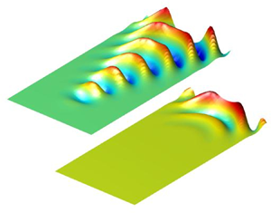
Another motivation for the current work is therefore to examine a much simplified problem involving just the linearised unsteady triple-deck equations, with the base flow being the linear shear profile. By doing this we can study the evolution of the perturbations using a similar numerical technique to that of Logue et al. (Reference Logue, Gajjar and Ruban2014) to see whether anything new can be learnt about the wave packets that arise in the simulations, and whether the unexplained difficulties can be resolved. The Terent'ev (Reference Terent'ev1984) vibrator problem, or the generalisation of it with localised heating as adopted here, is one such simpler problem where it is also possible to obtain a solution using analytical means. Here we use a Fourier–Laplace transform to solve the initial-value problem and obtain the analytical results in addition to solving the same equations numerically. The results presented in the current work demonstrate that a wave packet, emanating from the forced response, grows to large amplitudes very quickly, as indeed also seen in the experiments of Gaster & Grant (Reference Gaster and Grant1975). The numerical difficulties in resolving the wave packet occur because of the time steps used in the numerical solution were too large, as well as from the number of Fourier modes taken. By reducing the time steps used and working with a restricted range of wavenumbers in Fourier space, the signal can be resolved both spatially and temporally.
In § 2 we derive the governing unsteady equations starting from the compressible Navier–Stokes equations and using the scalings appropriate to the lower-branch. The full motivation for using the chosen scalings and the inclusion of localised heating effects is given in other papers, see Koroteev & Lipatov (Reference Koroteev and Lipatov2009) and Aljohani & Gajjar (Reference Aljohani and Gajjar2017b) for instance, and so is not repeated here. The adoption of the scalings appropriate to the lower-branch instability of the boundary layer is linked to the objectives discussed previously. The problem formulation for flow over localised heating with upper-branch scalings can be obtained as a special case of the problem formulation by Gajjar (Reference Gajjar1996). In § 3 we discuss the analytical solution to the linearised unsteady equations using Fourier–Laplace transforms. In § 4 a numerical solution of the linearised unsteady equations is obtained via a time-stepping algorithm combining spectral collocation in the wall normal direction and solving for the individual wavenumbers in Fourier space. The numerical techniques used are very similar to those of Logue et al. (Reference Logue, Gajjar and Ruban2014). Finally, in § 5 we finish with some additional comments and conclusions.
2. Problem formulation
The problem we study here is a modified version of one first studied by Terent'ev (Reference Terent'ev1981). Consider the subsonic flow past a flat plate containing a vibrator at a distance  $L$ from the leading edge of the plate, see figure 1. The plate also contains a localised heating element whose dimensions are small compared with the thickness of the boundary layer. We assume that the Reynolds number
  $Re$ is large (where
  $Re={\rho _{\infty }U_{\infty }L/\mu _{\infty }}$). At large distances from the plate the flow is uniform with speed
  $U_{\infty }$ parallel to the plate and with density
  $\rho _{\infty }$ and
  $\mu _{\infty }$ is the dynamic viscosity coefficient. We assume that the flow is two-dimensional and neglect any variations in the spanwise direction.

Figure 1. Boundary layer flow over a flat plate with speed  $U_{\infty }$ at large distances from the plate. A vibrator is located at a distance
  $L$ from the leading edge and with an oncoming boundary layer flow represented by
  $U_B$.
We non-dimensionalise the variables and flow quantities with respect to a lengthscale  $L$, velocity
  $U_{\infty }$, and free-stream density
  $\rho _{\infty }$ so that
 \begin{equation} \left.\begin{gathered} x=\frac{x^{*}}{L}, \quad y=\frac{y^{*}}{L},\quad t=\frac{U_{\infty}}{L}t^{*}, \quad u=\frac{u^{*}}{U_{\infty}},\quad v=\frac{v^{*}}{U_{\infty}},\quad T= \frac{{T}^{*}}{T_{\infty}},\\ p=\frac{p^{*}-p_{\infty}}{\rho_{_{\infty}}U_{\infty}^{2}},\quad \mu=\frac{\mu^{*}}{\mu_{\infty}} \quad \textrm{and} \quad \rho=\frac{\rho^{*}}{\rho_{\infty}}. \end{gathered}\right\} \end{equation}
The superscript asterisk quantities are dimensional,  $(x,y)$ are the coordinates in the streamwise and wall normal direction with corresponding velocity components
  $(u,v),$
  $t$ is time,
  $T$ is the temperature,
  $p$ the pressure,
  $\mu$ the dynamic viscosity,
  $\rho$ is the density and
  $p_{\infty }$ is the free-stream pressure.
In addition to the Reynolds number  $Re$ we have the Prandtl number
  $Pr,$ the specific gas constant
  $\mathcal {R}$ and
  $M_{\infty }$ the free-stream Mach number. Here,
  $M_{\infty }= {U_{\infty }}/{c_{\infty }}$ where
  $c_{\infty }=\sqrt {\gamma p_{\infty }/\rho _{\infty }}$ is the speed of sound in the undisturbed flow and
  $\gamma$ is the ratio of specific heats, and
  $T_{\infty }=U_{\infty }^{2} /(M_{\infty }^{2} \mathcal {R} \gamma )$.
We assume that the vibrator oscillates with a frequency  $\varOmega$ and has a maximum amplitude
  $b$ in the transverse direction. The vibrator is confined to a distance
  $a$ in the streamwise direction. Although it is possible to consider different scenarios, we restrict our attention to the case when
  $b=O(Re^{-5/8})$ and
  $a=O(Re^{-3/8})$. These are precisely the triple-deck scalings which, as shown by Smith (Reference Smith1979), capture the asymptotic properties of the dominant Tollmien–Schlichting wave instability in the boundary layer. With this choice of scales it is possible to make further progress using analytical techniques. Starting with the triple-deck structure also allows other distinguished limits to be studied as limiting cases of the current problem. Lipatov (Reference Lipatov2006) has suggested additional possibilities which arise from choosing different scalings for
  $a$ and
  $b$ when localised surface heating is present.
We need additionally to decide on the time scale to be used in the analysis. Choosing the time scale such that the unsteady terms appear at the same time as nonlinearity in the wall layer would appear to the most natural starting point. Other distinguished scales may then be deduced via limiting cases. Suppose  ${\rm \Delta} u$ denotes the perturbation to the oncoming flow, and
  ${\rm \Delta} x=O(Re^{-3/8})$ is the streamwise extent of the perturbation. If we balance the unsteady and inertial terms in the wall layer we find that
 \begin{equation} \frac{\partial u }{\partial t} \sim u\frac{\partial u }{\partial x} \end{equation}
gives
 \begin{equation} \frac{{\rm \Delta} u }{\varDelta t} \sim u \frac{{\rm \Delta} u }{{\rm \Delta} x}, \end{equation}
where  ${\rm \Delta} t$ denotes the scale of the unsteady variations in the wall layer. The streamwise velocity perturbation in the lower deck is
  $u\sim {\rm \Delta} u= O(Re^{-{1}/{8}})$.
Hence,
 \begin{equation} {\rm \Delta} t \sim \frac{{\rm \Delta} x }{u} \sim \frac{Re^{-{3}/{8}} }{Re^{-{1}/{8}}} = Re^{-{1}/{4}} . \end{equation}
 With the scalings given previously, the vibrator is situated near  $x=1$ and, hence, we may set
  $x=1+Re^{-{3/8}} x_{*}$ where
  $x_*$ is
  $O(1)$ in the region occupied by the vibrator. We model the vibrator by some function
  $y=y_w(t,x)$ with
 \begin{equation} y=y_w(t,x)=Re^{-{5/8}}f(t_*,x_*) , \end{equation}
and the function  $f(t_*,x_*)$ describes the spatial distribution of the localised disturbance caused by the vibrator. Specific forms of
  $f(t_*,x_*)$ are considered later, but it is assumed that
  $f(t_*,x_*)$ is zero apart from a small interval in the vicinity of the vibrator.
The presence of the vibrator means that at the wall we require that
 \begin{equation} u=0, \quad v=\frac{\partial y_w }{\partial t} \quad \textrm{on}\ y=y_w(t,x). \end{equation}
 In view of the earlier comments regarding scalings we set the frequency of oscillation  $\varOmega ={ \omega _0^{*}} Re^{{1/4}}$, where
  ${\omega _0^{*}}$ is taken to be an
  $O(1)$ scaled frequency parameter. Let
  $t=Re^{-{1}/{4}}t_*$ and
  $t_*$ is
  $O(1)$.
Next we assume that there is also a localised heating element on the flat plate co-located with the vibrator. This is modelled by the wall temperature profile being given by  $T= T_w(t_*,x_*)$ on
  $y=y_w$.
Unsteady effects notwithstanding, the analysis leading to the reduced governing equations follows closely that of the steady problem of subsonic flow over a localised heated element as in Aljohani & Gajjar (Reference Aljohani and Gajjar2017b) and so are not repeated here. The fundamental problem reduces to solving the triple-deck equations in the lower deck, see figure 2, where (with  $y=Re^{-5/8}y_3$) the flow quantities are expanded as
 \begin{gather} u(t,x,y;Re)=Re^{-{1/8}}u_*(t_*,x_*,y_3)+ \dots, \end{gather}
 \begin{gather}v(t,x,y;Re)=Re^{-{3/8}}v_3(t_*,x_*,y_3)+ \dots, \end{gather}
 \begin{gather}p(t,x,y;Re)= Re^{-{1/4}}p_*(t_*,x_*,y_3)+ \dots , \end{gather}
 \begin{gather}\rho(t,x,y;Re)= \rho_*(t_*,x_*,y_3)+ \dots, \end{gather}
 \begin{gather}T(t,x,t;Re)=T_*(t_*,x_*,y_3)+ \dots . \end{gather}
Figure 2. Schematic diagram showing the vibrator, triple-deck region and oncoming boundary layer flow. Region 1 with  $y=Re^{-3/8}y_1$ is the upper deck, region 2 with
  $y=Re^{-1/2}y_2$ is the main part of the boundary layer and region 3 with
  $y=Re^{-5/8}y_3$ the lower deck. The oncoming boundary flow just ahead of the vibrator is represented by region 4.
Substitution into the Navier–Stokes, the continuity equation, the energy equation and the equation of state gives
 \begin{gather} \frac{\partial \rho_* }{\partial t_*}+\frac{\partial (\rho_* u_*)}{\partial x_*}+ \frac{\partial (\rho_* v_3)}{\partial {y_3}} =0 \end{gather}
 \begin{gather}\rho_*\left(\frac{\partial {u}_* }{\partial t_*}+ {u}_*\frac{\partial {u}_*}{\partial x_*}+ {v}_3 \frac{\partial {u}_*}{\partial {y_3}}\right)= -\frac{\partial {p}_*}{\partial x_*} + \frac{\partial }{\partial y_3}\left(\mu_*\frac{\partial {u}_*}{\partial y_3}\right), \end{gather}
 \begin{gather}0 = -\frac{\partial {p}_*}{\partial {y_3}}, \end{gather}
 \begin{gather}\rho_*\left(\frac{\partial {T}_* }{\partial t_*}+ {u}_*\frac{\partial {T}_*}{\partial x_*}+ {v}_3 \frac{\partial {T}_*}{\partial {y_3}}\right)= \frac{1}{Pr}\frac{\partial}{\partial y_3}\left (\mu_*\frac{\partial {T}_*}{\partial y_3}\right) , \end{gather}
 \begin{gather}\rho_*T_* = (\gamma M_{\infty}^{2})^{-1}. \end{gather}
The boundary conditions are
 \begin{gather} v_3(t_*,x_*,y_3)=\frac{\partial f}{\partial t_*}\quad \textrm{on} \ y_3=f(t_*,x_*), \end{gather}
 \begin{gather}u_*(t_*,x_*,y_3)=0 \quad \textrm{on}\ y_3=f(t_*,x_*), \end{gather}
 \begin{gather}T_*(t_*,x_*,y_3)=T_w(t_*,x_*) \quad \textrm{on}\ y_3=f(t_*,x_*), \end{gather}
 \begin{gather}u_*(t_*,x_*,y_3)= \lambda y_3 \quad \textrm{as}\ x_* \to -\infty , \end{gather}
 \begin{gather}A_*(t_*,x_*)= 0\quad \textrm{as}\ x_* \to -\infty , \end{gather}
 \begin{gather}T_*(t_*,x_*,y_*)= (\gamma M_{\infty}^{2})^{-1} \quad \textrm{as}\ x_* \to -\infty , \end{gather}
 \begin{gather}u_*(t_*,x_*,y_3)=\lambda (y_3 + A_*(t_*,x_*)) \quad \textrm{as}\ y_3 \to \infty , \end{gather}
 \begin{gather}T_*(t_*,x_*,y_*)= (\gamma M_{\infty}^{2})^{-1} \quad \textrm{as}\ y_3\to \infty , \end{gather}
with  $\lambda ={\partial U_B(1,y)}/{\partial y}|_{y=0}$ being the reduced shear of the oncoming boundary layer flow
  $u=U_B(x_*,Re^{1/2}y)$, and
  $A_*$ is an unknown displacement function. Note that even though the boundary conditions (2.9f) and (2.9h) suggest that the temperature is constant when merging with oncoming flow, the temperature does vary in the lower-deck interaction region as governed by (2.8d) and is also not constant in region 4 where there is a thermal boundary layer.
These equations are coupled with the following upper-deck (region 1) problem, which is the same as in the steady case (see, for example, Stewartson Reference Stewartson1974):
 \begin{equation} (1-M_{\infty}^{2})\frac{\partial^{2} p_1}{\partial x_*^{2}} +\frac{\partial^{2} p_1 }{\partial y_1^{2}} = 0, \end{equation}
with  $y = Re^{-3/8}y_1$ and the pressure has been expanded as
 \begin{equation} p =Re^{-{1/4}}p_1(t_*,x_*,y_1)+ \cdots . \end{equation}
The problem for  $p_1$ is to be solved together with the matching conditions
 \begin{equation} p_1(t_*,x_*,y_1=0)=p_*(t_*,x_*), \quad \left.\frac{\partial p_1 }{\partial y_1}\right|_{y_1=0} = \frac{\partial^{2} A_*(t_*,x_*)}{\partial x^{2}_*} ,\end{equation}
and far-field conditions
 \begin{equation} p_*(t_*,x_*,y_1) \to 0 {\quad} \textrm{as}\ x_*^{2}+y_1^{2} \to \infty. \end{equation}
We first make use of the combined unsteady Dorodnitsyn–Howarth transform followed by the Prandtl transposition given by
 \begin{equation} t_*,x_*, y_*\to t_*,x_*,\quad y_*(t_*,x_*,y_3) = \int_{f(t_*,x_*)}^{y_3}\rho(t_*,x_*,y_3)\,\textrm{d}y_3 , \end{equation}
and
 \begin{equation} \rho_*v_3 = v_* -\frac{\partial y_*}{\partial t_*}-u_*\frac{\partial y_* }{\partial x_*} . \end{equation}
The form of the transform given previously with the lower limit non-zero is an extension of the usual unsteady Dorodnitsyn–Howarth transform, which is discussed in van Dyke (Reference van Dyke1952) for the one-dimensional case and Neiland et al. (Reference Neiland, Bogolepov, Dudin and Lipatov2007) for the two-dimensional case. The equations (2.8) and boundary conditions (2.9) reduce (see appendix A for details) to
 \begin{gather} \frac{\partial {u}_*}{\partial x_*}+ \frac{\partial { v}_*}{\partial {y_*}} =0 \end{gather}
 \begin{gather}\frac{\partial {u}_* }{\partial t_*}+ {u}_*\frac{\partial {u}_*}{\partial x_*}+ {v}_* \frac{\partial {u}_*}{\partial {y_*}}= -T_*(\gamma M_{\infty}^{2})\frac{\partial {p}_*}{\partial x_*} + \frac{\partial}{\partial y_*}\left( \rho_*\mu_*\frac{\partial {u}_*}{\partial y_* }\right), \end{gather}
 \begin{gather}0 = -\frac{\partial {p}_*}{\partial {y_*}}, \end{gather}
 \begin{gather}\frac{\partial {T}_* }{\partial t_*}+ {u}_*\frac{\partial {T}_*}{\partial x_*}+ {v}_* \frac{\partial {T}_*}{\partial {y_*}}= \frac{1}{Pr}\frac{\partial}{\partial y_*}\left( \rho_*\mu_*\frac{\partial {T}_*}{\partial y_*}\right) , \end{gather}
 \begin{gather}\rho_*T_* = (\gamma M_{\infty}^{2})^{-1}. \end{gather}
The boundary conditions are
 \begin{gather} v_*(t_*,x_*,y_*)=0 \quad \textrm{on} \ y_*=0, \end{gather}
 \begin{gather}u_*(t_*,x_*,y_*)=0 \quad \textrm{on}\ y_*=0, \end{gather}
 \begin{gather}T_*(t_*,x_*,y_*)=T_w(t_*,x_*) \quad \textrm{on}\ y_*=0, \end{gather}
 \begin{gather}u_*(t_*,x_*,y_*)= \lambda y_* \quad \textrm{as}\ x_* \to -\infty , \end{gather}
 \begin{gather}u_*(t_*,x_*,y_*)=\lambda (y_* + K_*(t_*,x_*)) \quad \textrm{as}\ y_* \to \infty , \end{gather}
where
 \begin{equation} K_*(t_*,x_*)= f(t_*,x_*)+\int_0^{\infty}(\gamma M_{\infty}^{2} T_* -1)\,\textrm{d}y_* + A_*(t_*,x_*) . \end{equation}
The term involving the integral in the expression for  $K_*$ in (2.14f) represents the additional displacement effect produced by the wall heating.
In what follows, we use the Chapman viscosity law expressed by  $\mu _*= C T_*$ for some constant
  $C$. This and additional constants such as
  $\lambda , \gamma , M_{\infty }$ appearing in the equations given previously may be effectively removed with the aid of the following affine transformation:
 \begin{equation} \left.\begin{gathered} t_*=\beta^{1/2} \lambda^{-3/2}C^{-1/2}(\gamma M_{\infty}^{2})^{1/2}\tau, \quad x_*=\beta^{3/4}\lambda^{-5/4} (\gamma M_{\infty}^{2})^{1/4}C^{-1/4} X,\\ y_*=\lambda^{-3/4}\beta^{1/4}C^{1/4}(\gamma M_{\infty}^{2})^{-1/4} Y, \quad y_1=\lambda^{-5/4}\beta^{7/4}C^{-1/4}(\gamma M_{\infty}^{2})^{1/4} {\bar Y},\\ u_*=\lambda^{1/4} \beta^{1/4}C^{1/4}(\gamma M_{\infty}^{2})^{-1/4} U, \quad v_*=\lambda^{3/4} C^{3/4}\beta^{-1/4}(\gamma M_{\infty}^{2})^{-3/4}V,\\ p_*=\beta^{1/2} \lambda^{1/2}C^{1/2}(\gamma M_{\infty}^{2})^{-1/2} P, \quad T_*= (\gamma M_{\infty}^{2})^{-1}\theta , \quad p_1= \beta^{1/2} \lambda^{1/2}C^{1/2}(\gamma M_{\infty}^{2})^{-1/2} P_1,\\ A_*=\lambda^{-3/4}\beta^{1/4}C^{1/4}(\gamma M_{\infty}^{2})^{-1/4}A,\quad K_*=\lambda^{-3/4}\beta^{1/4}C^{1/4}(\gamma M_{\infty}^{2})^{-1/4}K ,\\ f=\lambda^{-3/4}\beta^{1/4}C^{1/4}(\gamma M_{\infty}^{2})^{-1/4}F,\quad T_w=(\gamma M_{\infty}^{2})^{-1}\theta_w , \end{gathered}\right\} \end{equation}
and we have put  $\beta =(1-M_{\infty }^{2})^{-1/2}$. After using the transformation in (2.13)–(2.14) in conjunction with the Chapman viscosity law and the equation of state the resulting equations are given by
 \begin{gather} \frac{\partial {U}}{\partial X}+ \frac{\partial {V}}{\partial {Y}} =0 , \end{gather}
 \begin{gather}\frac{\partial {U} }{\partial \tau}+ {U}\frac{\partial {U}}{\partial X}+ {V} \frac{\partial {U}}{\partial {Y}}= -\theta \frac{\partial {P}}{\partial X} + \frac{\partial^{2} {U}}{\partial {Y}^{2}}, \end{gather}
 \begin{gather}0 = -\frac{\partial {P}}{\partial {Y}} , \end{gather}
 \begin{gather}\frac{\partial {\theta} }{\partial \tau}+ {U}\frac{\partial {\theta}}{\partial X}+ {V} \frac{\partial {\theta}}{\partial {Y}}= \frac{1}{Pr}\frac{\partial^{2} {\theta}}{\partial {Y}^{2}}. \end{gather}
 \begin{gather} V(\tau,X,Y)=0 \quad \textrm{on} \ Y=0, \end{gather}
 \begin{gather}U(\tau,X,Y)=0 \quad \textrm{on}\ Y=0, \end{gather}
 \begin{gather}\theta(\tau,X,Y)= \theta_w(\tau,X) \quad \textrm{on }\ Y=0, \end{gather}
 \begin{gather}U(\tau,X,Y)= Y \quad \textrm{as}\ X \to -\infty , \end{gather}
 \begin{gather}U(\tau,X,Y)=Y + K(\tau,X), \quad \textrm{as}\ Y \to \infty . \end{gather}
Here  $K$ is given by
 \begin{equation} K(\tau,X)=F(\tau,X)+\int_0^{\infty}(\theta(\tau,X,Y)-1)\,\textrm{d}Y + A(\tau,X) . \end{equation}
The transformed upper-deck problem is
 \begin{equation} \frac{\partial^{2} P_1 }{\partial X^{2}}+\frac{\partial^{2} P_1 }{\partial {\bar Y}^{2}}=0, \end{equation}
with the boundary conditions
 \begin{equation} \left.\begin{gathered} P_1 \to 0 {\quad} \textrm{as} \ (X^{2}+{\bar Y}^{2}) \to \infty ,\\ P_1(\tau,X,{\bar Y}=0)=P(\tau,X),\quad \frac{\partial P_1 }{\partial {\bar Y}}= \frac{\partial^{2} A}{\partial X^{2}} {\quad} \textrm{on} \ {\bar Y}=0 . \end{gathered}\right\} \end{equation}
Here  $F$ represents the transformed wall shape and
  $\theta _w$ is the prescribed heating profile and both these functions are assumed to be given.
The initial-value problem is supplemented with the initial conditions
 \begin{equation} U=Y,\quad \theta=\theta_w=1, \quad V,P,P_1,A,F = 0 \quad \textrm{for}\ \tau \leqslant 0 . \end{equation}
The nonlinear initial-value problem requires a numerical solution in general, but for small amplitudes of the vibrator we can find a linearised solution.
We assume that the wall motion and localised heating profiles are given by
 \begin{equation} \left.\begin{gathered} F(\tau,X)= \epsilon F_a(\tau,X)=\epsilon h(X)\sin(\omega_0 \tau) , \quad \tau >0 ,\\ \theta_w(\tau,X)=1+\epsilon g(\tau,X), \quad \tau >0 , \end{gathered}\right\} \end{equation}
where  $\epsilon$ represents the maximum amplitude of the oscillation and
  $\omega _0$ is some prescribed frequency. If
  $g=0$, then it reduces to the problem studied by Terent'ev (Reference Terent'ev1984).
2.1. Fourier–Laplace solution for small  $\epsilon$

For  $0<\epsilon \ll 1$ we may expand the flow quantities as
 \begin{gather} U(\tau,X,Y)= Y + \epsilon U_a(\tau,X,Y) + O(\epsilon^{2}), \end{gather}
 \begin{gather}V(\tau,X,Y)=\epsilon V_a(\tau,X,Y)+ O(\epsilon^{2}), \end{gather}
 \begin{gather}\theta(\tau,X,Y)= 1 + \epsilon \theta_a(\tau,X,Y) + O(\epsilon^{2}), \end{gather}
 \begin{gather}P(\tau,X)= \epsilon P_a(\tau,X) + O(\epsilon^{2}), \end{gather}
 \begin{gather}P_1(\tau,X,{\bar Y})=\epsilon P_u(\tau,X,{\bar Y})+ O(\epsilon^{2}), \end{gather}
 \begin{gather}A(\tau,X)= \epsilon A_a(\tau,X) + O(\epsilon^{2}), \end{gather}
 \begin{gather}K(\tau,X)= \epsilon K_a(\tau,X) + O(\epsilon^{2}). \end{gather}
Substituting (2.21) into (2.16)–(2.18b) and linearising for small  $\epsilon$ leads to the following linearised initial-value problem
 \begin{gather} \frac{\partial {U_a}}{\partial X}+ \frac{\partial {V_a}}{\partial {Y}} =0 , \end{gather}
 \begin{gather}\frac{\partial {U_a} }{\partial \tau}+ {Y}\frac{\partial {U_a}}{\partial X}+ {V_a} =-\frac{\partial {P_a}}{\partial X} + \frac{\partial^{2} {U_a}}{\partial {Y}^{2}}, \end{gather}
 \begin{gather}0 = -\frac{\partial {P_a}}{\partial {Y}} , \end{gather}
 \begin{gather}\frac{\partial {\theta_a} }{\partial \tau}+ {Y}\frac{\partial {\theta_a}}{\partial X} = \frac{1}{Pr}\frac{\partial^{2} {\theta_a}}{\partial {Y}^{2}} , \end{gather}
 \begin{gather}K_a=h(X)\sin(\omega_0 \tau)+ A_a+\int_0^{\infty}\theta_a \, \textrm{d}Y , \end{gather}
where
 \begin{gather} U_a(\tau,X,Y=0)=0, \end{gather}
 \begin{gather}V_a(\tau,X,Y=0)=0 , \end{gather}
 \begin{gather}\theta_a(\tau,X,Y=0)= g(\tau,X), \end{gather}
 \begin{gather}U_a=V_a=\theta_a=K_a=P_a=A_a=0 \quad \textrm{for}\ \tau \leqslant 0, \end{gather}
 \begin{gather}U_a(\tau,X,Y)= 0 \quad \textrm{as}\ X \to -\infty , \end{gather}
 \begin{gather}U_a(\tau,X,Y)= K_a(\tau,X)\quad \textrm{as}\ Y \to \infty , \end{gather}
and
 \begin{equation} \frac{\partial^{2} P_u }{\partial X}+\frac{\partial^{2} P_u }{\partial {\bar Y}^{2}}=0, \end{equation}
with the boundary conditions
 \begin{equation} \left.\begin{gathered} P_u \to 0 {\quad} \textrm{as} \ (X^{2}+{\bar Y}^{2}) \to \infty ,\\ P_u(\tau,X,{\bar Y}=0)=P_a(\tau,X),\quad \frac{\partial P_u }{\partial {\bar Y}}= \frac{\partial^{2} A_a}{\partial X^{2}} {\quad} \textrm{on} \ {\bar Y}=0. \end{gathered}\right\} \end{equation}
Let us introduce the Fourier–Laplace transform
 \begin{equation} U_a^{ \dagger \dagger}(\omega,k,Y)=\int_0^{\infty} \int_{-\infty}^{\infty}U_a(\tau,X,Y) \exp({-\omega \tau -\textrm{i} k X})\, \textrm{d}X\,\textrm{d}\tau \end{equation}
and the corresponding inverse by
 \begin{equation} U_a(\tau,X,Y)=\frac{1}{{4{\rm \pi}^{2} \textrm{i}}}\int_{-\infty}^{\infty}\int_\mathcal{L} U_a^{ \dagger \dagger}(\omega,k,Y)\exp({\omega \tau+\textrm{i} k X})\,\textrm{d}\omega\, \textrm{d}k , \end{equation}
with similar expressions for the other quantities. The double superscript denotes the Fourier–Laplace transform and the single superscript the Fourier transform. In addition,  $\mathcal {L}$ is a vertical line in the complex
  $\omega$ plane to the right of all singularities of the transform functions to satisfy causality.
Taking transforms of (2.22) and (2.23) gives
 \begin{gather} \textrm{i}k U_a^{ \dagger \dagger}+\frac{\partial V_a^{ \dagger \dagger}}{\partial Y}=0, \end{gather}
 \begin{gather}(\textrm{i}kY +\omega) U_a^{ \dagger \dagger} + V_a^{ \dagger \dagger}=-\textrm{i}kP_a^{ \dagger \dagger}+ \frac{\partial^{2} U_a^{ \dagger \dagger} }{\partial Y^{2}} , \end{gather}
 \begin{gather}(\textrm{i}kY +\omega) \theta_a^{ \dagger \dagger} =\frac{1}{Pr} \frac{\partial^{2} \theta_a^{ \dagger \dagger} }{\partial Y^{2}} . \end{gather}
The equation (2.27c) for the temperature perturbation may be solved in terms of Airy functions to obtain the solution
 \begin{equation} \theta_a^{ \dagger \dagger}= D_0 { {{\textrm{Ai}}}}(Pr^{1/3}\xi)+D_1{ {{\textrm{Bi}}}}(Pr^{1/3}\xi) ,\end{equation}
where
 \begin{equation} \xi=(\textrm{i}k)^{1/3}Y + \xi_0, \quad \xi_0=\omega(\textrm{i}k)^{-{2/3}} . \end{equation}
We take a branch cut along the positive imaginary axis so that  $-3{\rm \pi} /2 <\arg (k)< {\rm \pi}/2$. Then the function
  $Bi(\xi )$ grows exponentially when
  $Y \to \infty$ and, hence,
  $D_1$ must be zero. Application of the boundary conditions yields
 \begin{equation} \theta_a^{ \dagger \dagger}= g^{ \dagger \dagger}(k,\omega)\frac{{ {{\textrm{Ai}}}}(Pr^{1/3}\xi) }{{ {{\textrm{Ai}}}}(\eta_0)},\end{equation}
where we have written
 \begin{equation} \eta_0=Pr^{1/3}\xi_0.\end{equation}
 Next differentiating (2.27b) with respect to  $Y$ and using the continuity equation shows that
 \begin{equation} \frac{\partial^{3} U_a^{ \dagger \dagger}}{\partial Y^{3}}-(\textrm{i}kY+\omega)\frac{\partial U_a^{ \dagger \dagger} }{\partial Y}=0 . \end{equation}
This has the solution
 \begin{equation} \frac{\partial U_a^{ \dagger \dagger}}{\partial Y}= C_0 { {{\textrm{Ai}}}}(\xi)+ C_1 { {{\textrm{Bi}}}}(\xi). \end{equation}
The Airy function  $\textrm {Bi}(\xi )$ grows exponentially for large
  $Y$ and so we must take
  $C_1=0$. Setting
  $Y=0$ in (2.27b) and using (2.33) gives
 \begin{equation} (\textrm{i}k)^{1/3}C_0 { {{\textrm{Ai}}}}'(\xi_0)= \textrm{i}k P_a^{ \dagger \dagger} . \end{equation}
We can further integrate (2.33) to obtain
 \begin{equation} U_a^{ \dagger \dagger}=C_0(\textrm{i}k)^{-{1/3}}\int_{\xi_0}^{\xi}{ {{\textrm{Ai}}}}(\xi)\,\textrm{d}\xi . \end{equation}
Letting  $Y\to \infty$ in (2.35) and using the transformed boundary conditions from (2.23) shows that
 \begin{equation} K_a^{ \dagger \dagger}= C_0 (\textrm{i}k)^{-{1/3}}\int_{\xi_0}^{\infty}{ {{\textrm{Ai}}}}(\xi)\,\textrm{d}\xi . \end{equation}
We also have from (2.22e)
 \begin{equation} K_a^{ \dagger \dagger}= A_a^{ \dagger \dagger}+\int_{0}^{\infty}\theta_a^{ \dagger \dagger}\,\textrm{d}Y +\frac{h^{ \dagger}(k) \omega_0 }{(\omega^{2}+\omega_0^{2})}, \end{equation}
which after using the solution for  $\theta _a^{ \dagger \dagger }$ becomes
 \begin{equation} K_a^{ \dagger \dagger}= A_a^{ \dagger \dagger}+g^{ \dagger \dagger}(\textrm{i}kPr)^{-1/3}\int_{\eta_0}^{\infty}\frac{{ {{\textrm{Ai}}}}(\eta) }{ { {{\textrm{Ai}}}(\eta_0)}}\,\textrm{d}\eta +\frac{h^{ \dagger}(k) \omega_0 }{(\omega^{2}+\omega_0^{2})} . \end{equation}
 The equations for  $P_u$ do not involve
  $\tau$ explicitly and, therefore, taking Fourier–Laplace transforms of (2.24a) and applying the boundary conditions gives the usual relation,
 \begin{equation} P_a^{ \dagger \dagger}=\frac{k^{2} }{|k|}A_a^{ \dagger \dagger} . \end{equation}
Finally, eliminating  $C_0$ and solving for
  $P_a^{ \dagger \dagger }$ from (2.34), (2.36) and (2.39) gives
 \begin{equation} P_a^{ \dagger \dagger}(k,\omega)=P_{\pm}^{ \dagger \dagger}(\omega,k) = \frac{H^{ \dagger \dagger}(k,\omega) \omega_0 |k| { {{\textrm{Ai}}}}'(\xi_0) }{(\omega^{2}+\omega_0^{2}) D^{\pm}(\xi_0,k)}, \end{equation}
where  $\xi _0$ is defined in (2.29a,b) and
 \begin{equation} D^{\pm}(\xi_0,k)= -{ {{\textrm{Ai}}}}'(\xi_0) \pm k(\textrm{i}k)^{1/3}\int_{\xi_0}^{\infty}{ {{\textrm{Ai}}}}(\xi)\,\textrm{d}\xi , \end{equation}
with the plus sign in  $D^{\pm }$ corresponding to
  $k$ positive and the minus sign for
  $k$ negative. In this expression we have defined
 \begin{equation} H^{ \dagger \dagger}(k,\omega)=h^{ \dagger}(k)+ g^{ \dagger \dagger}(k,\omega)\frac{(\omega^{2}+\omega_0^{2})(\textrm{i}k Pr)^{-1/3}\int_{\eta_0}^{\infty} { {{\textrm{Ai}}}}(\eta)\,\textrm{d}\eta }{ \omega_0 { {{\textrm{Ai}}}}(\eta_0)}. \end{equation}
 The disturbed pressure  $P_a(\tau ,X)$ is calculated by formally inverting (2.40).
A number of results are immediately apparent from (2.40). Note that if we have no localised heating and set  $g^{ \dagger \dagger }$ to be zero, then (2.40) reduces to the expression obtained by Terent'ev (Reference Terent'ev1984). Somewhat more interesting is that, even without a vibrator, localised heating is also able to excite Tollmien–Schlichting waves (as also discussed in the following). With a vibrator present, if the localised heating profile is chosen such that
  $H^{ \dagger \dagger }=0$, then the response
  $P_a^{ \dagger \dagger }$ is zero, which means no Tollmien–Schlichting waves. In fact, the required localised heating profile is given by
  $g^{ \dagger \dagger }(\omega ,k)=g_{TC}^{ \dagger \dagger }$ where
 \begin{equation} g_{TC}^{ \dagger \dagger}(\omega,k)=-\frac{h^{ \dagger}(k) \omega_0 { {{\textrm{Ai}}}}(\eta_0)(\textrm{i}k Pr)^{1/3} }{ (\omega^{2}+\omega_0^{2})\int_{\eta_0}^{\infty}{ {{\textrm{Ai}}}}(\eta)\,\textrm{d}\eta} . \end{equation}
The expression (2.43) is significant and potentially gives a means by which it is possible to control instabilities in the boundary layer. Some typical results emanating from this formula are shown later in the paper.
2.2. Inverse transform to find the pressure $P_a(\tau ,X)$

Applying the inverse transform to  $P_a^{ \dagger \dagger }$ given by (2.40) shows that
 \begin{align} P_a(\tau,X)&=P(\tau,X)=\frac{1}{{4{\rm \pi}^{2} \textrm{i}}}\left[ \int_{-\infty}^{0} \int_\mathcal{L} P_{-}^{ \dagger \dagger}(k,\omega)\exp({\textrm{i}kX+\omega \tau}) \,\textrm{d}\omega\, \textrm{d}k\right. \end{align}
 \begin{align} &\quad +\left. \int_0^{\infty}\int_{\mathcal{L}}P_{+}^{ \dagger \dagger}(k,\omega) \exp({\textrm{i}kX+\omega \tau})\, \textrm{d}\omega\,\textrm{d}k\right]. \end{align}
We further write
 \begin{equation} P_{\pm}^{ \dagger \dagger}= P_{\pm}^{(V) \dagger \dagger}+P_{\pm}^{(H) \dagger \dagger} \end{equation}
with
 \begin{equation} P_{\pm}^{(V) \dagger \dagger}=\frac{h^ \dagger(k) \omega_0 |k| { {{\textrm{Ai}}}}'(\xi_0)}{(\omega^{2}+\omega_0^{2}) D^{\pm}(\xi_0,k)}, \quad P_{\pm}^{(H) \dagger \dagger}= \frac{{ {{\textrm{Ai}}}}'(\xi_0)|k|(\textrm{i}k Pr)^{-1/3} g^{ \dagger \dagger}(k,\omega)\int_{\eta_0}^{\infty}{ {{\textrm{Ai}}}}(\eta)\, \textrm{d}\eta }{{ {{\textrm{Ai}}}}(\eta_0) D^{\pm}(\xi_0,k)} . \end{equation}
The superscripts  $(V)$ and
  $(H)$ separate out the effects due to the vibrator and localised heating. Consider first
 \begin{equation} P_{-}^{(V)}(\tau,X)= \frac{1}{{4{\rm \pi}^{2}}\textrm{i} }\int_{-\infty}^{0} \int_\mathcal{L} P_-^{(V) \dagger \dagger}(k,\omega) \exp({\textrm{i}kX + \omega \tau})\, \textrm{d}\omega\,\textrm{d}k . \end{equation}
2.3. Inversion of the pressure $P_-^{(V)}$ the vibrator contribution

In the complex  $\omega$ plane the integrand has poles at
  $\omega =\pm \textrm {i} \omega _0$ and at the zeros of
  $D^{-}(\xi _0,k)=0.$ In figure 3(a) the first few zeros are shown for
  $k$ varying from
  $-\infty$ to zero. Suppose that we label the roots
  $\omega _{1,j}$
  $(j=1,2,\dots )$, then for
  $j=2,3,\dots$ the roots have the property that
  $\textrm {Re}(\omega _{1,j})<0$. Only the root
  $\omega _{1,1}$ crosses the imaginary axis into the first quadrant when
  $k=k^{*}$ and with
  $\omega _{1,1}(k_*)=\textrm {i}\omega ^{*}$. The properties of the roots of the dispersion relation
  $D^{\pm }(\xi _0,k)=0$ have been studied in many papers including Terent'ev (Reference Terent'ev1981, Reference Terent'ev1984), Walker, Fletcher & Ruban (Reference Walker, Fletcher and Ruban2006) and Ruban, Bernots & Kravtsova (Reference Ruban, Bernots and Kravtsova2016). In order to evaluate the inner integral in (2.48) we deform the contour
  $\mathcal {L}$ into the left-hand
  $\omega$ plane as shown in figure 4. Using Cauchy's theorem
 \begin{align} &\frac{1}{2{\rm \pi} \textrm{i}}\left(\int_{L}+ \int_{C_1+C_2+C_R}\right) P_-^{(V) \dagger \dagger}{\exp({\textrm{i}kX+\omega \tau}})\,\textrm{d}\omega \nonumber\\ &\quad = \sum[\text{Residues of}\ P_-^{(V) \dagger \dagger}{\exp({\textrm{i}kX+\omega \tau})} \ \text{inside the contour}\ \mathcal{L}+{C_1+C_2+C_R} ]. \end{align}
The residues arise from poles at  $\omega =\pm \textrm {i} \omega _0$ and when
  $\omega =\omega _{1,j}$. Hence,
 \begin{align} &\frac{1}{2{\rm \pi} \textrm{i}}\left(\int_{L}+ \int_{C_1+C_2+C_R}\right)P_-^{(V) \dagger \dagger} \exp({\textrm{i}kX+\omega \tau})\,\textrm{d}\omega\nonumber\\ &\quad =\frac{|k| h^{ \dagger}(k){ {{\textrm{Ai}}}}'(\xi_0(\textrm{i}\omega_0,k))}{2 \textrm{i} D^{-}(\xi_0(\textrm{i}\omega_0,k),k)} \exp({\textrm{i}\omega_0 \tau+ \textrm{i} k X}) \nonumber\\ &\qquad -\frac{|k| h^{ \dagger}(k){ {{\textrm{Ai}}}}'(\xi_0(-\textrm{i}\omega_0,k))}{2 \textrm{i} D^{-}(\xi_0(-\textrm{i}\omega_0,k),k)}\exp({-\textrm{i}\omega_0 \tau+ \textrm{i} k X})\nonumber\\ &\qquad + \sum_j \frac{|k|\omega_0 h^{ \dagger}(k){ {{\textrm{Ai}}}}' (\xi_0(\omega_{1,j},k))}{(\omega_0^{2}+\omega_{1,j}^{2}) \dfrac{\partial D^{-} }{\partial \omega}(\xi_0(\omega_{1,j},k),k)} \exp({\omega_{1,j} \tau+ \textrm{i} k X}) . \end{align}
The integrals  $\int _{C_1}, \int _{C_2}, \int _{C_R}$ can be shown to tend to zero when
  $R \to \infty$. Hence,
 \begin{align} P_-^{(V)}(\tau,X)&= \frac{1}{{2{\rm \pi}}}\int_{-\infty}^{0} \frac{|k| h^{ \dagger}(k){ {{\textrm{Ai}}}}'(\xi_0(\textrm{i}\omega_0,k))}{2 \textrm{i} D^{-}(\xi_0(\textrm{i}\omega_0,k),k)}\exp({\textrm{i}\omega_0 \tau+ \textrm{i} k X}) \, \textrm{d}k \nonumber\\ &\quad - \frac{1}{{2{\rm \pi}}}\int_{-\infty}^{0}\frac{|k| h^{ \dagger}(k){ {{\textrm{Ai}}}}'( \xi_0(-\textrm{i}\omega_0,k))}{2 \textrm{i} D^{-}(\xi_0(-\textrm{i}\omega_0,k),k)}\exp({-\textrm{i}\omega_0 \tau+ \textrm{i} k X}) \, \textrm{d}k \nonumber\\ &\quad + \frac{1}{{2{\rm \pi}}}\sum_j \int_{-\infty}^{0} \frac{|k|\omega_0 h^{ \dagger}(k){ {{\textrm{Ai}}}}'( \xi_0(\omega_{1,j},k))}{(\omega_0^{2}+\omega_{1,j}^{2}) \dfrac{\partial D^{-} }{\partial \omega}(\xi_0(\omega_{1,j},k),k)}\exp({\omega_{1,j}(k) \tau+ \textrm{i} k X}) \, \textrm{d}k . \end{align}
Figure 3. Locus of the roots (a)  $\omega _{1,j}$ of
  $D^{-}(\xi _0,k)=0$ for
  $k$ varying from
  $(-\infty ,0)$ and (b)
  $\omega _{2,j}$ of
  $D^{+}(\xi _0,k)=0$ with
  $k$ varying from
  $(0,\infty )$. The labels correspond to the different roots
  ${\omega _{1,j}},{\omega _{2,j}}$,
  $j=1,2,\ldots$.

Figure 4. Deformed contour for inversion of the integral in the  $\omega$-plane.
The calculation can be repeated for the inversion of  $P_+^{(V){ \dagger \dagger }}$ and the details are very similar to those described previously and give
 \begin{align} P_+^{(V)}(\tau,X)&= \frac{1}{{2{\rm \pi}}}\int^{\infty}_0 \frac{|k| h^{ \dagger}(k){ {{\textrm{Ai}}}}'(\xi_0(\textrm{i}\omega_0,k))}{2 \textrm{i} D^{+}(\xi_0(\textrm{i}\omega_0,k),k)}\exp({\textrm{i}\omega_0 \tau+ \textrm{i} k X}) \, \textrm{d}k\nonumber\\ &\quad - \frac{1}{{2{\rm \pi}}}\int^{\infty}_0\frac{|k| h^{ \dagger}(k){ {{\textrm{Ai}}}}'(\xi_0(-\textrm{i}\omega_0,k))}{2 \textrm{i} D^{+}(\xi_0(-\textrm{i}\omega_0,k),k)}\exp({-\textrm{i}\omega_0 \tau+ \textrm{i} k X}) \, \textrm{d}k\nonumber\\ &\quad + \frac{1}{{2{\rm \pi}}}\sum_j \int^{\infty}_0 \frac{|k|\omega_0 h^{ \dagger}(k){ {{\textrm{Ai}}}}'(\xi_0(\omega_{2,j},k))}{(\omega_0^{2}+\omega_{2,j}^{2}) \dfrac{\partial D^{+} }{\partial \omega}(\xi_0(\omega_{2,j},k),k)}\exp({\omega_{2,j}(k) \tau+ \textrm{i} k X} )\, \textrm{d}k . \end{align}
In (2.52) we have labelled  $\omega _{2,j}(k)$ as the zeros of
  $D^{+}(\xi _0,k)=0$ for
  $k$ positive.
2.4. Inversion of the pressure $P_{-}^{(H)}$ the localised heating contribution

As  $P_-^{(H)}$ involves the function
  $g^{ \dagger \dagger }(\omega ,k)$ many profiles could be chosen, but suppose we take a localised heating profile of the form
 \begin{equation} g(\tau,x)={\hat g}(x)\sin(\omega_0\tau), \end{equation}
giving
 \begin{equation} g^{ \dagger \dagger}(\omega,k)=\frac{{\hat g}^{ \dagger}(k) \omega_0}{\omega^{2}+\omega^{2}_0}. \end{equation}
Then
 \begin{equation} P_{\pm}^{(H) \dagger \dagger}= \frac{{ {{\textrm{Ai}}}}'(\xi_0)|k|(\textrm{i}k Pr)^{-1/3} {\hat g}^{ \dagger}(k)\omega_0\int_{\eta_0}^{\infty}{ {{\textrm{Ai}}}}(\eta)\,\textrm{d}\eta }{(\omega^{2}+\omega_0^{2}){ {{\textrm{Ai}}}}(\eta_0) D^{\pm}(\xi_0,k)} . \end{equation}
In inverting the transform  $P_{\pm }^{(H) \dagger \dagger }$ in addition to the poles discussed when inverting
  $P_{\pm }^{(V) \dagger \dagger }$ we also have additional poles, which we label as
  $\omega =\omega _{3,j}(k),\omega _{4,j}(k)$, arising from the zeros of
  ${ {{\textrm {Ai}}}}(\eta _0)$ in the denominator of (2.55). The Airy function
  ${ {{\textrm {Ai}}}}(\eta _0)$ has zeros on the negative real axis and we can write
 \begin{equation} \eta_0 = -|a_j| \quad (j=1,2,\dots) \end{equation}
where  $a_j$ is a zero of the Airy function
  ${ {{\textrm {Ai}}}}(\eta )$. Using the definition of
  $\eta _0$ from (2.29a,b) and (2.31) we obtain
 \begin{equation} \omega(k)=\omega_{3,j}= \frac{|a_j k^{2/3}|}{Pr^{1/3}} \exp({-4\textrm{i}{\rm \pi}/3}) \quad (k<0), \end{equation}
and
 \begin{equation} \omega(k)=\omega_{4,j} =\frac{|a_j k^{2/3}|}{Pr^{1/3}} \exp({-2\textrm{i}{\rm \pi}/3}) \quad (k>0). \end{equation}
As the real part of  $\omega _{3,j}(k), \omega _{4,j}(k)$ is negative these do not contribute to any additional unstable modes. The inversion follows a similar argument to that already given and it can be shown that
 \begin{align} &2{\rm \pi} P_-^{(H)}(\tau,X) \nonumber\\ &\quad = \int_{-\infty}^{0} \frac{ {\hat g}^{ \dagger}(k)|k|^{2/3}\,\textrm{e}^{{\textrm{i}{\rm \pi}}/{{6}}}(Pr)^{-1/3}{ {{\textrm{Ai}}}}'(\xi_0(\textrm{i}\omega_0,k)) \int_{\eta_0(\textrm{i}\omega_{0},k)}^{\infty}{ {{\textrm{Ai}}}}(\eta)\,\textrm{d}\eta }{2 \textrm{i} { {{\textrm{Ai}}}}(\eta_0(\textrm{i}\omega_0,k))D^{-}(\xi_0(\textrm{i}\omega_0,k),k)}\exp({\textrm{i}\omega_0 \tau+ \textrm{i} k X}) \, \textrm{d}k \nonumber\\ &\qquad - \int_{-\infty}^{0}\frac{ {\hat g}^{ \dagger}(k)|k|^{2/3}\,\textrm{e}^{{\textrm{i}{\rm \pi}}/{{6}}}(Pr)^{-1/3}{ {{\textrm{Ai}}}}'( \xi_0(-\textrm{i}\omega_0,k)) \int_{\eta_0(-\textrm{i}\omega_0,k)}^{\infty}{ {{\textrm{Ai}}}}(\eta)\,\textrm{d}\eta }{2 \textrm{i} { {{\textrm{Ai}}}}(\eta(-\textrm{i}\omega_0,k))D^{-}(\xi_0(-\textrm{i}\omega_0,k),k)}\nonumber\\ &\qquad \times\exp({-\textrm{i}\omega_0 \tau+ \textrm{i} k X}) \, \textrm{d}k \nonumber\\ &\qquad +\sum_j \int_{-\infty}^{0} \frac{\omega_0 {\hat g}^{ \dagger}(k) |k|^{2/3} \,\textrm{e}^{{\textrm{i}{\rm \pi}}/{{6}}}(Pr)^{-1/3}{ {{\textrm{Ai}}}}'(\xi_0(\omega_{1,j},k))\int_{\eta_0(\omega_{1,j},k)}^{\infty}{ {{\textrm{Ai}}}}(\eta)\,\textrm{d}\eta }{(\omega_0^{2}+\omega_{1,j}^{2}) { {{\textrm{Ai}}}}(\eta_0(\omega_{1,j},k)) \dfrac{\partial D^{-} }{\partial \omega}(\xi_0(\omega_{1,j},k),k)}\nonumber\\ &\qquad\times \exp({\omega_{1,j}(k) \tau+ \textrm{i} k X}) \, \textrm{d}k \nonumber\\ &\qquad + \sum_j \int_{-\infty}^{0} \frac{\omega_0 {\hat g}^{ \dagger}(k){ {{\textrm{Ai}}}}'(\xi_0(\omega_{3,j},k))|k|^{4/3} \,\textrm{e}^{-{\textrm{i}{\rm \pi}}/{{6}}}(Pr)^{-2/3}\int_{\eta_0(\omega_{3,j},k)}^{\infty}{ {{\textrm{Ai}}}}(\eta)\,\textrm{d}\eta }{(\omega_ 0^{2}+\omega_{3,j}^{2}) { {{\textrm{Ai}}}}'(\eta_0(\omega_{3,j},k)){D^{-} }(\xi_0(\omega_{3,j},k),k)}\nonumber\\ &\qquad \times\exp({\omega_{3,j}(k) \tau+ \textrm{i} k X}) \, \textrm{d}k . \end{align}
 An expression for  $P_+^{(H)}$ may be derived in a similar manner.
Finally,
 \begin{equation} P(\tau,X)= P_-(\tau,X)+P_+(\tau,X) . \end{equation}
To interpret the findings, we need the following additional results.
First note that if we write  $k=|k| \,\textrm {e}^{\textrm {i}\theta _k}$ where
  $\theta _k$ is the argument of
  $k$, then
  $\xi _0(\omega ,k)$ can be written as
 \begin{equation} {\xi_0(\omega,k)}= {\omega (\textrm{i}k)^{-2/3}} = \omega |k|^{-2/3}\exp({-2\textrm{i}\theta_k/3})\exp({-\textrm{i}{\rm \pi}/3}). \end{equation}
Hence, the complex conjugate of  $\xi _0(\omega ,k)$ is
 \begin{equation} [\xi_0(\omega,k)]^{(c)}= \omega^{(c)}|k|^{-2/3} \exp({2\textrm{i}\theta_k/3})\exp({\textrm{i}{\rm \pi}/3} ). \end{equation}
However, note that
 \begin{align} \xi_0(\omega^{(c)},k^{(c)}\exp({-\textrm{i}{\rm \pi}}))&= \omega^{(c)}|k|^{-2/3}\exp({2\textrm{i}(\theta_k+{\rm \pi})/3})\exp({-\textrm{i}{\rm \pi}/3})\nonumber\\ &= \omega^{(c)}|k|^{-2/3}\exp({2\textrm{i}\theta_k/3})\exp({\textrm{i}{\rm \pi}/3}) . \end{align}
This shows that
 \begin{equation} [\xi_0(\omega,k)]^{(c)}=\xi_0(\omega^{(c)},k^{(c)}\,\textrm{e}^{-\textrm{i}{\rm \pi}}) . \end{equation}
Using this, we observe that if  $D^{-}(\xi _0(\omega ,k))=0$, then taking the complex conjugate
 \begin{align} [D^{-}(\xi_0(\omega,k),k)]^{(c)} &=-{ {{\textrm{Ai}}}}'(\xi_0^{(c)})- |k|^{4/3}\exp\left({-\frac{4}{3}\textrm{i}\theta_k}\right)\exp({-\textrm{i}{\rm \pi}/6}) \int_{\xi_0^{(c)}}^{\infty}{ {{\textrm{Ai}}}}(\xi)\,\textrm{d}\xi ,\nonumber\\ &= -{ {{\textrm{Ai}}}}'(\xi_0^{(c)}) + |k|\exp\left({\textrm{i}\left(\frac{4}{3}\right)(-{\rm \pi}-\theta_k)}\right) \exp({\textrm{i}{\rm \pi} /6})\int_{\xi_0^{(c)}}^{\infty}{ {{\textrm{Ai}}}}(\xi)\,\textrm{d}\xi ,\nonumber\\ &= D^{+}(\xi_0(\omega^{(c)},k^{(c)}\exp({-\textrm{i}{\rm \pi}})),k^{(c)}\,\exp({-\textrm{i}{\rm \pi}}) ). \end{align}
Thus, if  $(\omega ,k)$ is a root of
  $D^{-}=0$, then
  $(\omega ^{(c)},k^{(c)}\,\textrm {e}^{-\textrm {i}{\rm \pi} })$ is a root of
  $D^{+}=0$; figure 3 confirms this observation. We can use these results to rewrite the inverted pressure as
 \begin{align} P(\tau,X) & = \frac{1}{{\rm \pi}}\textrm{Re} \left [ \int_{-\infty}^{0} \frac{|k| h^{ \dagger}(k){ {{\textrm{Ai}}}}'(\xi_0(\textrm{i}\omega_0,k))}{ 2 \textrm{i} D^{-}(\xi_0(\textrm{i}\omega_0,k),k)} \exp({\textrm{i}\omega_0 \tau+ \textrm{i} k X}) \, \textrm{d}k \right. \nonumber\\ &\quad -\int_{-\infty}^{0}\frac{|k| h^{ \dagger}(k){ {{\textrm{Ai}}}}'(\xi_0(-\textrm{i} \omega_0,k))}{ 2 \textrm{i} D^{-}(\xi_0(-\textrm{i}\omega_0,k),k)}\exp({-\textrm{i}\omega_0 \tau+ \textrm{i} k X}) \, \textrm{d}k \nonumber\\ &\quad + \sum_j \int_{-\infty}^{0} \frac{|k|\omega_0 h^{ \dagger}(k){ {{\textrm{Ai}}}}'(\xi_0(\omega_{1,j},k))}{ (\omega_0^{2}+\omega_{1,j}^{2}) \dfrac{\partial D^{-} }{ \partial \omega}(\xi_0(\omega_{1,j},k),k)} \exp({\omega_{1,j}(k) \tau+ \textrm{i} k X}) \, \textrm{d}k \nonumber\\ &\quad + \int_{-\infty}^{0} \frac{ {\hat g}^{ \dagger}(k)|k|^{2/3}\,\textrm{e}^{{\textrm{i}{\rm \pi}}/{{6}}}(Pr)^{-1/3}{ {{\textrm{Ai}}}}' (\xi_0(\textrm{i}\omega_0,k)) \int_{\eta_0(\textrm{i}\omega_{0},k)}^{\infty}{ {{\textrm{Ai}}}}(\eta)\,\textrm{d}\eta }{ 2 \textrm{i} { {{\textrm{Ai}}}}(\eta_0(\textrm{i}\omega_0,k))D^{-}(\xi_0(\textrm{i}\omega_0,k),k)}\nonumber\\ &\quad \times\exp({\textrm{i}\omega_0 \tau+ \textrm{i} k X}) \, \textrm{d}k \nonumber\\ &\quad - \int_{-\infty}^{0}\frac{ {\hat g}^{ \dagger}(k)|k|^{2/3} \textrm{e}^{{\textrm{i}{\rm \pi}}/{{6}}}(Pr)^{-1/3}{ {{\textrm{Ai}}}}'(\xi_0(-\textrm{i}\omega_0,k)) \int_{\eta_0(-\textrm{i}\omega_0,k)}^{\infty}{ {{\textrm{Ai}}}}(\eta)\,\textrm{d}\eta }{ 2 \textrm{i} { {{\textrm{Ai}}}}(\eta(-\textrm{i}\omega_0,k))D^{-}(\xi_0(-\textrm{i}\omega_0,k),k)}\nonumber\\ &\quad \times \exp({-\textrm{i}\omega_0 \tau+ \textrm{i} k X}) \, \textrm{d}k \nonumber\\ &\quad + \sum_j \int_{-\infty}^{0} \frac{\omega_0 {\hat g}^{ \dagger}(k)|k|^{2/3} \, \textrm{e}^{{\textrm{i}{\rm \pi}}/{{6}}}(Pr)^{-1/3}{ {{\textrm{Ai}}}}'(\xi_0(\omega_{1,j},k))\int_{\eta_0(\omega_{1,j},k)}^{\infty}{ {{\textrm{Ai}}}}(\eta)\,\textrm{d}\eta }{(\omega_0^{2}+\omega_{1,j}^{2}) { {{\textrm{Ai}}}}(\eta_0(\omega_{1,j},k)) \dfrac{\partial D^{-} }{\partial \omega}(\xi_0(\omega_{1,j},k),k)}\nonumber\\ &\quad\times\exp({\omega_{1,j}(k) \tau+ \textrm{i} k X} )\, \textrm{d}k \nonumber\\ &\quad + \sum_j \int_{-\infty}^{0} \frac{\omega_0 {\hat g}^{ \dagger}(k) |k|^{4/3} \,\textrm{e}^{-{\textrm{i}{\rm \pi}}/{{6}}}(Pr)^{-2/3}{ {{\textrm{Ai}}}}'(\xi_0(\omega_{3,j},k)) \int_{\eta_0(\omega_{3,j},k)}^{\infty} { {{\textrm{Ai}}}}(\eta)\,\textrm{d}\eta }{(\omega_0^{2}+\omega_{3,j}^{2}) { {{\textrm{Ai}}}}'(\eta_0(\omega_{3,j},k)){ D^{-} }(\xi_0 (\omega_{3,j},k),k)}\nonumber\\ &\quad\times\left. \vphantom{\sum_j \int_{-\infty}^{0}}\exp({\omega_{3,j}(k) \tau+ \textrm{i} k X}) \, \textrm{d}k \right]. \end{align}
 Note that the integrals in (2.66) (with terms multiplied by  $\exp ({\pm \textrm {i}\omega _0 \tau })$) represent the response due to the forcing at the vibrator frequency. The other terms are the response due to the excited modes of the boundary layer. For large time
  $\tau$ all the terms in the summations except that with
  $j=1$ corresponding to the root
  $\omega _{1,j}$ decay rapidly. If
  $j=1$, the integrands proportional to
  $\exp ({\omega _{1,j}\tau })$ have a simple pole at
  $k=k_1$ when
  ${\omega _{1,1}(k_1)}=\textrm {i}\omega _0$. The locus of the root
  ${\omega _{1,1}(k)}=\textrm {i}\omega _0$ in the complex
  $k$ plane for varying
  $\omega _0$ is shown in figure 5. When
  $\omega _0=\omega ^{*}=2.298$ and
  $k=k^{*}=-1.005$ the root crosses from the second quadrant into the third quadrant in the
  $k$ plane giving rise to unstable waves. In fact, we can estimate the terms by making use of Laplace's method and noting that the major contribution to the integrals come from the vicinity of
  $k=0$. The details of the lengthy calculation are omitted but are similar to those given by Terent'ev (Reference Terent'ev1984) and Ruban et al. (Reference Ruban, Bernots and Kravtsova2016) for instance. It is found that for large
  $\tau$ we can approximate (2.66) by
 \begin{align} P(\tau,X) & = \textrm{Re} \left[\frac{1}{{\rm \pi}} \int_{-\infty}^{0} \frac{|k| h^{ \dagger}(k){ {{\textrm{Ai}}}}'(\xi_0(\textrm{i}\omega_0,k))}{2 \textrm{i} D^{-}(\xi_0(\textrm{i}\omega_0,k),k)} \exp({\textrm{i}\omega_0 \tau+ \textrm{i} k X} )\, \textrm{d}k\right.\nonumber\\ &\quad -\frac{1}{{\rm \pi}} \int_{-\infty}^{0}\frac{|k| h^{ \dagger}(k){ {{\textrm{Ai}}}}'(\xi_0(-\textrm{i}\omega_0,k))}{2 \textrm{i} D^{-}(\xi_0(-\textrm{i}\omega_0,k),k)} \exp({-\textrm{i}\omega_0 \tau+ \textrm{i} k X}) \, \textrm{d}k \nonumber\\ &\quad + \frac{1}{{\rm \pi}} \int_{-\infty}^{0} \frac{ {\hat g}^{ \dagger}(k){ {{\textrm{Ai}}}}'(\xi_0(\textrm{i}\omega_0,k)) {|k|^{2/3}\,\textrm{e}^{{\textrm{i}{\rm \pi}}/{{6}}}(Pr)^{-1/3}} \int_{\eta_0(\textrm{i}\omega_{0},k)}^{\infty}{ {{\textrm{Ai}}}}(\eta)\,\textrm{d}\eta }{2 \textrm{i} { {{\textrm{Ai}}}}(\eta_0(\textrm{i}\omega_0,k))D^{-}(\xi_0(\textrm{i}\omega_0,k),k)}\nonumber\\ &\quad \times \exp({\textrm{i}\omega_0 \tau+ \textrm{i}k X}) \, \textrm{d}k \nonumber\\ &\quad -\frac{1}{{\rm \pi}} \int_{-\infty}^{0}\frac{ {\hat g}^{ \dagger}(k){ {{\textrm{Ai}}}}'(\xi_0(-\textrm{i}\omega_0,k)){|k|^{2/3}\,\textrm{e}^{{\textrm{i}{\rm \pi}}/{{6}}}(Pr)^{-1/3} } \int_{\eta_0(-\textrm{i}\omega_0,k)}^{\infty}{ {{\textrm{Ai}}}}(\eta)\,\textrm{d}\eta }{ 2 \textrm{i} { {{\textrm{Ai}}}}(\eta(-\textrm{i}\omega_0,k))D^{-}(\xi_0(-\textrm{i}\omega_0,k),k)}\nonumber\\ &\quad \times \exp({-\textrm{i}\omega_0 \tau+ \textrm{i} k X}) \, \textrm{d}k \nonumber\\ &\quad - \frac{|k_1| h^{ \dagger}(k_1){ {{\textrm{Ai}}}}'(\xi_0(\textrm{i}\omega_0,k_1)) }{ {\dfrac{\partial D^{-} }{\partial \omega}(\xi_0(\textrm{i}\omega_0,k_1),k_1) \dfrac{\textrm{d}\omega_{1,1} }{\textrm{d}k}(k_1)}}\exp({{\omega_{1,1}(k_1)} \tau+ \textrm{i} k_1 X} )\mathcal{H}(\omega_0-\omega^{*})\nonumber\\ &\quad - \frac{ {\hat g}^{ \dagger}(k_1)|k|^{2/3}\,\textrm{e}^{{\textrm{i}{\rm \pi}}/{{6}}}(Pr)^{-1/3}{ {{\textrm{Ai}}}}'(\xi_0(\textrm{i}\omega_{0},k_1)) \int_{\eta_0(\textrm{i}\omega_{0},k_1)}^{\infty}{ {{\textrm{Ai}}}}(\eta)\,\textrm{d}\eta }{ {{ {{\textrm{Ai}}}}(\eta_0(\textrm{i}\omega_{0},k_1))\dfrac{\partial D^{-} }{ \partial \omega}(\xi_0(\textrm{i}\omega_{0},k_1),k_1) \dfrac{\textrm{d}\omega_{1,j}}{\textrm{d}k}(k_1)}}\nonumber\\ &\quad \left.\vphantom{\int_{-\infty}^{0}}\times \exp({{\omega_{1,1}(k_1)} \tau+ \textrm{i} k_1 X}) \mathcal{H}(\omega_0-\omega^{*}) , \right] \end{align}
where  $\mathcal {H}(\theta )$ is the Heaviside function. The result (2.67) shows that for frequencies larger than the critical frequency
  $\omega ^{*}= 2.298$ the vibrator as well as localised heating is able to excite an unstable wave in the boundary layer whose shape and amplitude is given by the last two terms in (2.67). If we write the expression for the unstable wave in the form
 \begin{equation} J(\omega_0,k_1)\exp({{\omega_{1,1}}(k_1)\tau+ \textrm{i}k_1 X}), \end{equation}
then
 \begin{equation} J(\omega_0,k_1)=J_V(\omega_0,k_1) + J_H(\omega_0,k_1) \end{equation}
with
 \begin{gather} J_V(\omega_0,k_1)=-\textrm{Re}\left [ \frac{|k_1| h^{ \dagger}(k_1){ {{\textrm{Ai}}}}'(\xi_0( \textrm{i}\omega_0,k_1)) }{{ \dfrac{\partial D^{-} }{\partial \omega}(\xi_0(\textrm{i}\omega_0,k_1),k_1) \dfrac{\textrm{d}\omega_{1,1} }{\textrm{d}k}(k_1)}}\right], \end{gather}
 \begin{gather}J_H(\omega_0,k_1) =-\textrm{Re}\left[ \frac{ {\hat g}^{ \dagger}(k_1)|k|^{2/3} \,\textrm{e}^{{\textrm{i}{\rm \pi}}/{6}}(Pr)^{-1/3}{ {{\textrm{Ai}}}}'(\xi_0(\textrm{i}\omega_{0},k_1)) \int_{\eta_0(\textrm{i}\omega_{0},k_1)}^{\infty}{ {{\textrm{Ai}}}}(\eta)\,\textrm{d}\eta }{{{ {{\textrm{Ai}}}}(\eta_0( \textrm{i}\omega_{0},k_1))\dfrac{\partial D^{-} }{\partial \omega}(\xi_0(\textrm{i} \omega_{0},k_1),k_1) \dfrac{{\omega_{1,1}}}{\textrm{d}k}(k_1)}}\right]. \end{gather}
The terms  $J_V$,
  $J_H$ in (2.70) give the respective amplitudes of the generated Tollmien–Schlichting wave due to the vibrator and heating, respectively.

Figure 5. Locus of the root  $\omega _{1,1}(k)=\textrm {i}\omega _0$ with
  $\omega _0$ varying from
  $0$ to
  $\infty$. The arrow indicates the direction of
  $\omega _0$ increasing.
3. Numerical solution of the linearised triple-deck initial-value problem
As an alternative to the analytical solution of the previous section, here we focus on obtained results using a numerical approach to solving the initial-value problem. Consider the linearised triple-deck problem governed by (2.22), (2.23) and (2.27):
 \begin{gather} \frac{\partial U_a }{\partial X} + \frac{\partial {V_a} }{\partial Y}=0, \end{gather}
 \begin{gather}\frac{\partial U_a }{\partial \tau} + Y\frac{\partial U_a }{\partial X}+ V_a = -\frac{\partial P_a }{\partial X} + \frac{\partial^{2} U_a }{\partial Y^{2}}, \end{gather}
 \begin{gather}\frac{\partial \theta_a }{\partial \tau} + Y\frac{\partial {\theta_a} }{\partial X} = \frac{1}{Pr} \frac{\partial^{2} {\theta_a} }{\partial Y^{2}}, \end{gather}
for  $|X| < \infty$,
  $Y >0$ and
  $\tau >0$. The boundary and initial conditions are
 \begin{gather} U_a,V_a,\theta_a,P_a,A_a,K_a,F_a,\theta_{w}=0 \quad \tau<0, \end{gather}
 \begin{gather}U_a(\tau,X,Y=0)=V_a(\tau,X,Y=0)= 0, \end{gather}
 \begin{gather}K_a(\tau,X)=F_a(\tau,X)+A_a(\tau,X)+\int_0^{\infty}\theta_a(\tau,X,Y) \,\textrm{d}Y ,\quad \textrm{for} \ \tau>0, \end{gather}
 \begin{gather}U_a(\tau,X,Y\to \infty)= K_a(\tau,X), \end{gather}
 \begin{gather}U_a,V_a,P_a,A_a,\theta_a,K_a, \to 0 {\quad} \textrm{as} \ |X| \to \infty. \end{gather}
We also allow for more general wall-shape and heating functions, defined by
 \begin{equation} F_a(\tau,X)=h(X) q(\tau) , \quad \theta_{aw}=g(\tau,X) \quad 0<\tau . \end{equation}
The function  $h(X)$ is a smooth Gaussian hump given by
  $h(X)= \textrm {e}^{-X^{2}/4}$. Note that this is different from the triangular-shaped bump employed by Terent'ev (Reference Terent'ev1984), which was given by
 \begin{equation} h(X) = \left\{\begin{array}{l} 0 \quad X < 0 \ \textrm{or} \ X > 2,\\ X \quad \textrm{for} \ 0 < X < 1,\\ 2-X \quad \textrm{for} \ 1 < X < 2. \end{array} \right. \end{equation}
 As we discuss later, the use of (3.3) makes resolving the resulting flow substantially more challenging owing to the slow (algebraic) decay of the Fourier spectrum at high wavenumbers. For the function  $q(\tau )$ the work of Terent'ev (Reference Terent'ev1984) and the analytical results given previously use
  $q(\tau )=\sin \omega _0 \tau$. For the numerical work we have used
  $q(\tau )=\sin \omega _0 \tau$ as well as a smoother initial start given by
 \begin{equation} q(\tau)=(1-\textrm{e}^{-a\tau^{2}})\sin(\omega_0 \tau), \end{equation}
with  $a=1/10$. The choice of the wall heating functions
  $g(\tau ,X)$ used is discussed in the following.
We also have the relationship
To solve the set (3.1)–(3.5) and, in particular, to find the pressure  $P_a(X,T)$ we performed a numerical study of the equations using the following method. First define a Fourier transform of
  $U_a(\tau ,X,Y)$ by
 \begin{equation} U_a^{ \dagger}(\tau,k,Y)=\frac{1}{\sqrt{2{\rm \pi}}}\int_{-\infty}^{\infty}U_a(\tau,X,Y)\,\textrm{e}^{-\textrm{i}kX} \, \textrm{d}X . \end{equation}
The inverse is given by
 \begin{equation} U_a(\tau,X,Y)=\frac{1}{\sqrt{2{\rm \pi}}}\int_{-\infty}^{\infty}U_a^{ \dagger}(\tau,k,Y)\,\textrm{e}^{\textrm{i}kX} \, \textrm{d}X . \end{equation}
Then equations (3.1)–(3.5) become
 \begin{gather} \textrm{i}kU_a^{ \dagger} + \frac{\partial V_a^{ \dagger} }{\partial Y} = 0, \end{gather}
 \begin{gather}\frac{\partial U_a^{ \dagger} }{\partial \tau} + \textrm{i}kY U_a^{ \dagger} + V_a^{ \dagger} = -\textrm{i}k P_a^{ \dagger} + \frac{\partial^{2} U_a^{ \dagger} }{\partial Y^{2}}, \end{gather}
 \begin{gather}\frac{\partial \theta_a^{ \dagger} }{\partial \tau} + \textrm{i}kY \theta_a^{ \dagger} = \frac{1}{Pr}\frac{\partial^{2} \theta_a^{ \dagger} }{\partial Y^{2}}, \end{gather}
 \begin{gather}U_a^{ \dagger}(\tau,k,Y=0)=V_a(\tau,k,Y=0)=0, \quad \theta_a(\tau,k,Y=0)=g^{ \dagger}(\tau,k), \end{gather}
 \begin{gather}K_a^{ \dagger}(\tau,k)=q(\tau)h^{ \dagger}(k)+A_a^{ \dagger}(\tau,k)+\int_0^{\infty}\theta_a^{ \dagger}(\tau, k,Y)\,\textrm{d}Y \quad \textrm{for}\ \tau >0 . \end{gather}
 \begin{gather}U_a^{ \dagger}(\tau,k, Y\to \infty)= K_a^{ \dagger}(\tau,k), \end{gather}
 \begin{gather}P_a^{ \dagger}(\tau,k)=\frac{k^{2}}{|k|}A_a^{ \dagger}(\tau,k) . \end{gather}
 We use a second-order fully implicit time-differencing scheme with time step  $d\tau$ and (3.8b) for example replaced by
 \begin{equation} \frac{3U_a^{{ \dagger}(n+1)}-4U_a^{{ \dagger}(n)}+U_a^{{ \dagger}(n-1)} }{2 {\textrm{d}\tau}} + \textrm{i} k Y U_a^{{ \dagger}(n+1)}+ V_a^{{ \dagger}(n+1)}= -\textrm{i} k P_a^{{ \dagger}(n+1)}+ \frac{\partial^{2} U_a^{{ \dagger}(n+1)} }{\partial Y^{2}}, \end{equation}
and from (3.8a)  $V_a^{ \dagger }$ is given by
 \begin{equation} V_a^{{ \dagger}(n+1)}= -\textrm{i} k \int_0^{Y} U_a^{{ \dagger}(n+1)} \, \textrm{d}Y .\end{equation}
Here, for example,  $U_a^{{ \dagger }(n)} =U_a^{ \dagger }(\tau _n)$ where
  $\tau _n=n \,\textrm {d}\tau$. For the first time step we use a first-order fully implicit scheme. For a given time level
  $n$ we solve the system of equations for
  $U_a^{ \dagger },P_a^{ \dagger },\theta _a^{ \dagger }$ by using Chebychev collocation at the collocation points
 \begin{equation} Y=Y_j= \frac{Y_{max} }{2}\left (1-\cos\left (\frac{j {\rm \pi}}{N}\right )\right), \quad j=0, \dots, N \end{equation}
with the approximate outer boundary  $Y_{max}$ chosen suitably. Let
  ${\boldsymbol {u}^{{ \dagger }(\boldsymbol {n})}}= (u_j^{{ \dagger }(n)} )$ with
  $u_j^{{ \dagger }(n)}=U_a^{{ \dagger }(n)}(Y=Y_j),$ and similarly
  ${{\boldsymbol {\theta }}}^{{ \dagger }(n)}= (\theta _{aj}^{{ \dagger }(n)})$. Then (3.9) leads to a linear system of the form
 \begin{equation} {\boldsymbol{G}}\left(\begin{array}{c}{\boldsymbol{u}}^{{ \dagger}(n+1)}\\ A_a^{{ \dagger}(n+1)}\\ {{\boldsymbol{\theta}}}^{{ \dagger}(n+1)} \end{array}\right) ={\boldsymbol{R}}^{(n)}, \end{equation}
where  ${\boldsymbol {G}}$ is a square matrix of order
  $(2N+3)$ and
  ${\boldsymbol {R}}^{(n)}$ is the right-hand side of the linear system. To accommodate the boundary conditions we replace the first row of
  ${\boldsymbol {G}}$ with the condition from (3.8d)
 \begin{equation} u^{{ \dagger}(n+1)}(Y_0)= 0. \end{equation}
Row  $( N+1)$ of
  ${\boldsymbol {G}}$ is replaced by the boundary condition
 \begin{equation} u^{{ \dagger}(n+1)}(Y_{N})- A_a^{ \dagger(n+1)} -\int_0^{\infty}\theta_a^{{ \dagger}(n+1)}\, \textrm{d}Y= q(\tau_n)h^{ \dagger}(k), \end{equation}
making use of (3.8e). Row  $(N+2)$ of
  ${\boldsymbol {G}}$ is replaced by the condition stemming from the equation
 \begin{equation} \frac{\partial U_a^{ \dagger} }{\partial Y}(Y=Y_{N})=0 . \end{equation}
Finally, in row  $(N+3)$ and the last row of
  $G$ we use the remaining conditions on
  $\theta ^{ \dagger }$ at
  $Y=0$ and
  $Y=Y_{N}$, respectively.
For a given  $k$, we can solve the linear system (3.12) to find the unknown variables and, in particular,
  $P_a^{ \dagger (n)}(k)$. This is then inverted using the discrete inverse fast Fourier transform to obtain
  $P_a(\tau _n,X)$ and other quantities as required.
4. Results
Results are presented at various time intervals and for different frequencies. For the numerical work we have taken the Prandtl number  $Pr=1$. Figures 6, 7 and 8 show the pressure perturbation for
  $\omega =2$,
  $\omega =2.298$ and
  $\omega =2.5$, respectively, for the case when there is no heating. Unless otherwise specified, the values shown correspond to taking a time step
  ${\textrm {d}\tau }=T_{per}/256$ (with
  $T_{per}=2{\rm \pi} /\omega _0$),
  $N=32$,
  $Y_{max}=40$ and 2048 Fourier modes. The wall motion is described by
  $F_a(\tau ,X)=h(X)q(\tau )$ and
  $q(\tau )=\sin (\omega _0 \tau )$.

Figure 6. Results for the pressure perturbation with  $\omega _0=2$ (stable) at times
  $\tau = (K+\frac {1}{4})T_{per}$,
  $K=3,4,5,6,7,8,$ with
  ${g}(\tau ,X)=0$ (no heating).

Figure 7. Results for the pressure perturbation with  $\omega _0=2.298$ (neutral) at times
  $\tau = (K+\frac {1}{4})T_{per}$,
  $K=3,4,5,6,7,8$, with
  ${g}(\tau ,X)=0$ (no heating).

Figure 8. Results for the pressure perturbation with  $\omega _0=2.5$ (unstable) at times
  $\tau = (K+\frac {1}{4})T_{per}$,
  $K=3,4,5,6,7,8,$ with
  ${g}(\tau ,X)=0$ (no heating).
When  $\omega =2$ the analysis predicts a stable wave, when
  $\omega =2.298$ the wave is neutrally stable and when
  $\omega =2.5$ an unstable wave growing downstream with
  $X$ is generated. The numerical solutions in figures 6–8 are in accord with the predictions.
In figures 9–11 we present similar results but this time when there is no vibrator and only localised (unsteady) heating taking  $F_a=0$ and
  $g(\tau ,X)=h(X)q(\tau )$ and
  $q(\tau )=\sin (\omega _0\tau )$. The analytical results predict stable, neutral and unstable waves as before and as shown in the numerical results.

Figure 9. Results for the pressure perturbation with  $\omega _0=2$ (stable) at times
  $\tau = (K+\frac {1}{4})T_{per}$,
  $K=3,4,5,6,7,8$ and no vibrator, forced by unsteady heating.

Figure 10. Results for the pressure perturbation with  $\omega _0=2.298$ (neutral) at times
  $\tau = (K+\frac {1}{4})T_{per}$,
  $K=3,4,5,6,7,8$ and no vibrator, forced by unsteady heating.

Figure 11. Results for the pressure perturbation with  $\omega _0=2.5$ (unstable) at times
  $\tau = (K+\frac {1}{4})T_{per}$,
  $K=3,4,5,6,7,8$ and no vibrator, forced by unsteady heating.
In figure 12 we present the temperature perturbation  $\theta _a(\tau ,X,Y=Y_j)$ for the unstable case of
  $\omega =2.5$ at various times and with no vibrator (
 $F_a=0$) using the same localised heating function as in figure 11. Even though the frequency corresponds to the case of an unstable spatially (downstream) growing wave, the instability is confined to just the velocity and pressure field and not the temperature perturbation as predicted by the analysis.

Figure 12. Temperature profile  $\theta (X,Y_j,\tau )$ with
  $g(X,\tau )=h(X)q(\tau ), h(x)=0$ and
  $\omega =2.5$ with
  $Y_j\approx 7.759$ at times
  $\tau =(K+\frac {1}{4})T_{per}$,
  $K=3,4,5,6,7,8$.
4.1. Tollmien–Schlichting wave cancellation
In this section we present results showing Tollmien–Schlichting wave cancellation taking place with appropriately chosen localised temperature forcing. The analysis suggests that cancellation will take place provided that the wall forcing is chosen according to (2.43). We can formally invert this to find
 \begin{equation} g_{TC}(\tau,X) = -\frac{1}{4{\rm \pi}^{2} \textrm{i}}\int_{-\infty}^{\infty} \int_{L} \frac{h^{ \dagger}(k) \omega_0 { {{\textrm{Ai}}}}(\eta_0)(\textrm{i}kPr)^{1/3} }{ (\omega^{2}+\omega_0^{2}) \int_{\eta_0}^{\infty}{ {{\textrm{Ai}}}}(\eta)\,\textrm{d}\eta} \exp({\omega \tau+ \textrm{i} k X}) \, \textrm{d}\omega \, \textrm{d}k, \end{equation}
where  ${L}$ is a contour to the right of all singularities of the integrand in the complex
  $\omega$ plane. As far as the integral with respect to
  $\omega$ is concerned the integrand has poles at
  $\omega =\pm \textrm {i} \omega _0$ and when
 \begin{equation} \int_{\eta_0}^{\infty} { {{\textrm{Ai}}}}(\eta) \, \textrm{d}\eta =0. \end{equation}
The function  $\displaystyle {\int _z^{\infty }{ {{\textrm {Ai}}}}(\xi )\, \textrm {d}\xi }$ is the generalised Airy function and it is known that the zeros of this function form an infinite countable set and arise as complex conjugate pairs with negative real values. The first few such values are tabulated in table 1. If we label these zeros as
  $b_j=|b_j|\exp ({-\textrm {i}{\rm \pi} + \textrm {i}\psi _j})$, then from the definition
  $\eta _0$ we find that
 \begin{equation} \omega=\omega_{6j} = \frac{|b_j|\exp\left({-\dfrac{2{\rm \pi} \textrm{i}}{3} + \textrm{i} \psi_j}\right)(\textrm{i}k)^{2/3}}{Pr^{1/3}}. \end{equation}
Importantly we note from (4.3) that the real part of  $\omega _{6j}$ remains negative for
  $j=1,2,\dots$.
Table 1. First few zeros of  $\int _{\xi }^{\infty }{ {{\textrm {Ai}}}}(t)\,\textrm {d}t$ denoted by
  $b_j$. Note that these arise as complex conjugate pairs with negative real parts.

Hence, inverting the inner integral in (4.1) gives
 \begin{align} g_{TC}(\tau,X)&= -\frac{1}{2{\rm \pi}}\int_{-\infty}^{\infty}\frac{h^{ \dagger}(k){ {{\textrm{Ai}}}}(\eta( \textrm{i}\omega_0(k),k)) (\textrm{i}kPr)^{1/3}}{2 \textrm{i} \int_{\eta_0(\textrm{i}\omega_0,k)}^{\infty}{ {{\textrm{Ai}}}(\eta)\, \textrm{d}\eta}} \exp({\textrm{i}\omega_0\tau + \textrm{i}kX})\, \textrm{d}k \nonumber\\ &\quad + \frac{1}{2{\rm \pi}}\int_{-\infty}^{\infty}\frac{h^{ \dagger}(k){ {{\textrm{Ai}}}}(\eta(-\textrm{i}\omega_0(k),k))(\textrm{i} kPr)^{1/3} }{2 \textrm{i} \int_{\eta_0(-\textrm{i}\omega_0,k)}^{\infty}{ {{\textrm{Ai}}}(\eta)\,\textrm{d}\eta}} \exp({-\textrm{i}\omega_0\tau + \textrm{i}kX})\, \textrm{d}k \nonumber\\ &\quad + \sum_{j=1}^{\infty}\int_{-\infty}^{\infty}\frac{h^{ \dagger}(k) (\textrm{i}k)\omega_0 }{(\omega_0^{2} + \omega_{6j}^{2}) Pr^{1/3}} \exp({\omega_{6j}\tau+ \textrm{i} k X})\, \textrm{d}k. \end{align}
However, for the numerical computations, instead of the exact cancellation function given by (4.4) an approximation  $g_{TCN}(\tau ,X)$ was used, which is obtained by ignoring the terms in the summation. In the Fourier transform space the function
  $g^{ \dagger }_{TCN}(\tau ,k)$ is given by
 \begin{align} g^{{ \dagger}}_{TCN}(\tau,k)&= {h^{{ \dagger}}(k) \frac{(\textrm{i}kPr)^{1/3} {{\textrm{Ai}}}(\eta_0(-\textrm{i}\omega_0,k)) }{2\textrm{i}\int_{\eta_0(-\textrm{i}\omega_0,k)}^{\infty} { {{\textrm{Ai}}}}(\eta)\,\textrm{d}\eta} }\exp({-\textrm{i}\omega_0\tau})\nonumber\\ &\quad -{h^{{ \dagger}}(k) \frac{ {{\textrm{Ai}}}(\eta_0(\textrm{i}\omega_0,k))(\textrm{i}kPr)^{1/3} }{2\textrm{i} \int_{\eta_0(\textrm{i}\omega_0,k)}^{\infty} { {{\textrm{Ai}}}}(\eta)\,\textrm{d}\eta}} \exp({\textrm{i}\omega_0\tau}). \end{align}
In figure 13 we show the result of wave cancellation in action. The wall motion is taken to be the same as that for figure 8.

Figure 13. The pressure perturbation  $P_a(\tau ,X)$ with
  $\omega =2.5$ and Tollmien–Schlichting cancellation in action using the heating function given by (4.5) at times
  $\tau =(K+\frac {1}{4})T_{per}$,
  $K=3,4,5,6,7,8$.
In figure 14 we have compared wave cancellation with and without localised heating. Figures 14(a) and 15(a) show the effect on the amplitude of the wave at two instants in time, by choosing  $g(\tau ,X)$ according to (4.5). In figures 14(b) and 15(b) the comparison is over an extended range of
  $X$. In the earlier figures only a restricted range of
  $X$ is shown and this corresponds to the developing Tollmien–Schlichting wave. Over the extended range, the full response including a faster growing convective wave packet is clearly visible. This arises from the transient part of the signal and is present for all the cases (stable, neutral and unstable) studied, and it can be seen that the amplitude of the wave packet is orders of magnitude larger than the Tollmien–Schlichting wave amplitude. With wave cancellation using (4.5), the amplitude of this wave packet is diminished but remains significant as figure 14(b) shows.

Figure 14. Comparisons of the pressure perturbation with  $\omega =2.5$ at
  $T=(4+1/4)T_{per}$ with and without wave cancellation using (4.5): (a) for the restricted range in
  $x$ and in (b) over an extended range showing the wave packet.

Figure 15. Comparison of the pressure perturbations with  $\omega =2.5$ at
  $T=(8+1/4)T_{per}$ with and without wave cancellation using (4.5): (a) for restricted range in
  $x$ and in (b) over an extended range showing the wave packet.
In figure 16 the comparisons are also shown for the stable case with  $\omega _0=2$ and in figure 17 for the neutral case with
  $\omega =2.298$.

Figure 16. Comparison of the pressure perturbations at  $T=(8+1/4)T_{per}$ with and without wave cancellation using (4.5) for the stable case with
  $\omega _0=2$. (a) for restricted range in
  $x$ and in (b) over an extended range showing the wave packet.

Figure 17. Comparison of the pressure perturbations at  $T=(8+1/4)T_{per}$ with and without wave cancellation using (4.5) for the neutral case with
  $\omega _0=2.298$ (a) for restricted range in
  $X$ and in (b) over an extended range showing the wave packet.
The formula given by (4.4) predicts a complete cancellation of the signal, as seen in figures 15(a), 16(a), 17(a) for instance. However, on using the approximate formula in (4.5) although the Tollmien–Schlichting wave amplitude is reduced significantly, as seen by a comparison of figures 13 and 8, the wave packet amplitude is still very large, as figures 15(b), 16(b), 17(b) show.
It is possible that taking more terms in the expansion may help in reducing the amplitude of the wave packet but limitations arise because of numerical precision and roundoff errors. This is also one of the reasons why we chose the wall function to be a smooth Gaussian hump. With a triangular hump as used by Terent'ev (Reference Terent'ev1984) and given in (3.3), the computations were particularly sensitive to the growth of the high-wavenumber components affecting the wave packet amplitude. This can be seen in figure 18, which shows the Fourier transform amplitude as a function of the wavenumber at two times, comparing the results for the Gaussian hump with the triangular hump (3.3). Figure 18 initially shows two peaks, one near  $k=1$ corresponding to the Tollmien–Schlichting wave, and the other near
  $k=2.5$ in accordance with figure 3. For a triangular hump, the growth of the high-wavenumber components meant that computations and, in particular, the behaviour of the wave packet could not be adequately resolved after a short time. We restrict attention in these results to
  $|k| \leqslant 2{\rm \pi}$; the inclusion of a larger wavenumber range would require even further decreases of the temporal step in the numerical calculations.

Figure 18. Plots of the function  $|P^{ \dagger }(\tau ,k)|$ against
  $k$ at times
  $\tau =2T_{per}$ (dotted line) and
  $\tau =4T_{per}$ (solid line) for the Gaussian hump (labelled
  $G$) and triangular hump shape (labelled
  $Tr$).
Extensive grid size and other checks were carried out as documented in the accompanying supplementary material available at https://doi.org/10.1017/jfm.2020.928. It is noted that the wave packet amplitude is most sensitive to changes in the time steps  $\textrm {d}\tau$ and when using other integration schemes. Other parts of the signal including the Tollmien–Schlichting wave appear to be fully resolved when varying the grid parameters and time steps.
5. Conclusions
The most significant finding in this study is that we have shown that it is possible to chose a localised temperature profile that is able to cancel out Tollmien–Schlichting waves. A modified version of the exact heating profile was shown to be effective in radically reducing the amplitude of the unstable Tollmien–Schlichting wave generated. Although the analysis performed is linear and thus restricted to small amplitudes, it would be interesting to try applying the idea for a full nonlinear simulation. In principle, the same idea may be extended also for other situations including three-dimensional effects as well as Tollmien–Schlichting wave generation by other means. However, in a real flow Tollmien–Schlichting waves can be excited through multiple mechanisms and to be able to predict wave-cancellation profiles for a more general situation is a much more complex task. A number of problems for further study are suggested by the results presented here and in the first instance it would be interesting to revisit the experiments of Liepmann et al. (Reference Liepmann, Brown and Nosenchuck1982) and Liepmann & Nosenchuck (Reference Liepmann and Nosenchuck1982) using Navier–Stokes simulations, and incorporating the analytic formula for wave cancellation wall heating functions given here.
We have also calculated the receptivity coefficients due to Tollmien–Schlichting waves generated by the effects of wall vibration as well as localised heating for a special case of sinusoidal temporal forcing as given by the expressions (2.70a) and (2.70b).
The original motivation for the current study was the desire to fully understand the wave packets that caused difficulties in simulations of the unsteady triple-deck equations for nonlinear mean flows as in the work of Logue et al. (Reference Logue, Gajjar and Ruban2014) where also the wave packet was not fully resolved. By choosing to focus on a linear system where it is possible to proceed analytically as with the equations studied here, we have found that in order to resolve the wave packet in our linear system, extremely small time steps are required. The time steps used in Logue et al. (Reference Logue, Gajjar and Ruban2014) are much larger in comparison. We also found that the high-frequency spatial components are amplified because of the numerical techniques used, and the growth of these also leads to difficulties in performing long-time accurate computations.
Finally one other observation arising from the numerical results presented here is that the transient part of the signal leading to the formation of the downstream travelling wave packet has an order of magnitude larger amplitude as compared with the Tollmien–Schlichting wave amplitude. This is not too dissimilar to what is observed in the experimental studies by Gaster & Grant (Reference Gaster and Grant1975) where disturbances were introduced by impulsively injecting at some upstream location on the flat plate. This initiated a wave packet that propagated downstream. The frequency power spectrum in figure 2 of Gaster & Grant (Reference Gaster and Grant1975) shows two peaks as in our figure 18, and in the signal traces in figure 4 of Gaster & Grant (Reference Gaster and Grant1975), only the wave packet can be seen. The amplitude of the Tollmien–Schlichting wave excited is an order of magnitude smaller as their figure 2 also shows.
Acknowledgements
J.S.B.G. would like to thank Professor P. Hall (Monash University), Professor A. Ruban (Imperial College), Professor F.T. Smith (UCL) and Dr Y. Bhumkar (IIT Bhubaneshwar) for helpful suggestions and discussions on the work and the results presented in this paper. J.S.B.G. is also grateful to the Sydney Mathematics Research Institute (SMRI) at the University of Sydney for hosting a visit in 2019 where part of this work was completed. G.S.B. acknowledges the support provided by the EPSRC Centre for Doctoral Training in Industrially Focused Mathematical Modelling (EP/L015803/1). We would like to thank the referees for their useful and helpful comments which helped to improve the manuscript. One of the referees kindly directed us to the work of van Dyke (Reference van Dyke1952) and the relevant page in Neiland et al. (Reference Neiland, Bogolepov, Dudin and Lipatov2007) that helped us in improving the appendix when discussing the combined Prandtl–Dorodnitsyn–Howarth transformation.
Declaration of interests
The authors report no conflict of interest.
Supplementary material
Supplementary material is available at https://doi.org/10.1017/jfm.2020.928.
Appendix A. Combined Prandtl–Dorodnitsyn–Howarth transform
Following van Dyke (Reference van Dyke1952) and Neiland et al. (Reference Neiland, Bogolepov, Dudin and Lipatov2007), we introduce the change of variables  $(t_*,x_*,y_3) \to (T_*,X_*, y_*)$ where
 \begin{equation} T_*=t_*, \quad X_*=x_*, \quad y_*(t_*,x_*,y_3)= \int_{f(t_*,x_*)}^{y_3} \rho_*(t_*,x_*,y)\,{\textrm{d} y} , \end{equation}
and
 \begin{equation} \rho_* v_3 = v_* -\frac{\partial y_* }{\partial t_*}-u_*\frac{\partial y_* }{\partial x_*} . \end{equation}
Note that we have introduced the independent variables  $T_*=t_*, X_*=x_*$ for extra clarity in the following discussion, although in the main text we have retained
  $t_*$ and
  $x_*$ only.
The combined Prandtl–Dorodnitsyn–Howarth transformation given by (A 1a–c) and (A 2) and as used in the text, is a generalisation of the more familiar Dorodnitsyn–Howarth transform, see van Dyke (Reference van Dyke1952) and Neiland et al. (Reference Neiland, Bogolepov, Dudin and Lipatov2007), in which the lower limit in the integral for  $y_*$ is zero. Details of how this transform reduces the continuity equation to one without
  $\rho _*$, and how the boundary conditions at the wall
  $y_3=f$ are satisfied, are given in the following.
Using the transformation we have
 \begin{gather} \frac{\partial }{ \partial t_*} = \frac{\partial }{\partial T_*} + \frac{\partial y_* }{ \partial t_*}\frac{\partial }{ \partial y_*}, \end{gather}
 \begin{gather}\frac{\partial }{ \partial x_*} = \frac{\partial }{ \partial X_*} + \frac{\partial y_* }{ \partial x_*}\frac{\partial }{ \partial y_*}, \end{gather}
 \begin{gather}\frac{\partial }{ \partial y_3} = \rho_* \frac{\partial }{ \partial y_*}. \end{gather}
Next integrating the continuity equation (2.8a) and making use of the boundary conditions
 \begin{equation} u_*=0, \quad {v_3}=\frac{\partial f}{\partial t_*}, \quad \textrm{on} \ y_3=f(t_*,x_*), \end{equation}
we obtain
 \begin{equation} \rho_*v_3 = -\int_f^{y_3}\frac{\partial \rho_* }{\partial t_*}\,\textrm{d}y_3 - \int_f^{y_3}\frac{\partial }{\partial x_*}\left(\rho_* u_*\right) \textrm{d}y_3 + \rho(t_*,x_*,f)\frac{\partial f}{\partial t_*}(t_*,x_*) . \end{equation}
Next we make use of the Leibniz's rule for differentiation under the integral sign in (A 5) together with the boundary conditions in (A 4) to give
 \begin{align} \rho_*v_3 &= -\left[ \frac{\partial }{ \partial t_*}\left(\int_f^{y_3}\rho_* \,\textrm{d}y_3\right) + \rho_*(t_*,x_*,f)\frac{\partial f }{ \partial t_*}(t_*,x_*)\right]\nonumber\\ &\quad -\left[\frac{\partial }{ \partial x_*}\left(\int_f^{y_3} \rho_*u_*\,\textrm{d}y_3\right) + \rho_*(t_*,x_*,f)u_*(t_*,x_*,f)\frac{\partial f }{ \partial x_*}(t_*,x_*)\right] \nonumber\\ &\quad + \rho(t_*,x_*,f)\frac{\partial f}{\partial t_*}(t_*,x_*) \nonumber\\ &=-\frac{\partial y_* }{ \partial t_*}-\frac{\partial }{ \partial x_*} \left(\int_f^{y_3}\rho_* u_* \, \textrm{d}y_3\right) . \end{align}
We now introduce
 \begin{equation} u_* = \frac{\partial \varPsi }{\partial y_*} \end{equation}
and making use of the definition of  $y_*$, from (A 6) we have
 \begin{align} \rho_*v_3&= -\frac{\partial y_* }{ \partial t_*} -\frac{\partial }{ \partial x_*} \left(\int_0^{y_*} u_* \,\textrm{d}y_* \right)\nonumber\\ & = -\frac{\partial y_* }{ \partial t_*} -\frac{\partial \varPsi }{ \partial x_*}, \nonumber\\ &=-\frac{\partial y_* }{ \partial t_*} -\frac{\partial \varPsi }{ \partial X_*}-u_*\frac{\partial y_* }{ \partial x_*} . \end{align}
Combining (A 2) with the last result we find that
 \begin{equation} v_* = -\frac{\partial \varPsi }{\partial X_*}. \end{equation}
This now shows that the transformed continuity equation
 \begin{equation} \frac{\partial u_* }{\partial X_*} + \frac{\partial v_* }{\partial y_*}=0, \end{equation}
is satisfied. The definition of  $v_*$ in (A 2) also implies that
  $v_*=0$ on
  $y_3=f$ or
  $y_*=0$. Next the momentum equation (2.8b) together with the transformations (A 3) yields
 \begin{align} &\rho_*\left( \frac{\partial u_*}{ \partial T_*} + \frac{\partial y_* }{ \partial t_*}\frac{\partial u_*}{\partial y_*} +u_*\left( \frac{\partial u_*}{ \partial X_*} + \frac{\partial y_* }{ \partial x_*}\frac{\partial u_*}{\partial y_*}\right) +\rho_*v_3\frac{\partial u_* }{ \partial y_*}\right) \nonumber\\ &\quad = -\frac{\partial p_* }{ \partial X_*}-\frac{\partial y_* }{ \partial x_*}\frac{\partial p_*}{\partial y_*}+ \rho_* \frac{\partial }{\partial y_*} \left(\mu_* \rho_*\frac{\partial u_* }{\partial y_*}\right) \end{align}
which after using (A 2), (A 3c), (2.8c) and (2.8e) and noting that  $\partial p_* /\partial y_*=0$ reduces to (2.13b). The equation (2.8d) for
  $T_*$ is handled similarly.


