


1. Introduction
Phase-change materials (PCMs) are of interest in thermal management for their ability to store and release large amounts of energy near the phase transition temperature  $T_M$. PCMs with a suitable value of
  $T_M$ and a large heat of fusion can be effective in either active or passive thermal control systems and are used in a wide range of applications, including air conditioning, electronics, manufacturing, food storage, construction and the clean energy industry.
Space missions are a particularly interesting area for PCM applications because significant (undesired) temperature variations can result from the cycles of radiation exposure experienced by orbiting spacecraft or the waste heat generated by onboard systems. There is a long history of PCM use in space missions going back to the Apollo 15 Lunar Rover Vehicle, Skylab SL-1 and the Venera 8–10 missions of the Soviet Union (Lane & Shamsundar Reference Lane and Shamsundar1983; Creel Reference Creel2007). Future initiatives are also expected to benefit from the capability of PCMs to provide simple, passive and efficient thermal control. The ESA Moon Village programme, for example, will likely require managing the extreme temperature differences between the lunar day and night (Williams et al. Reference Williams, Paige, Greenhagen and Sefton-Nash2017).
Among the range of possible materials with appropriate operating temperatures for space applications, organic PCMs like alkanes are attractive due to their stability. Their effectiveness can be limited, however, by low thermal conductivity and the resulting lag in response time. One strategy for reducing the response time of the PCM device is to modify the effective thermal conductivity through the addition of more-conductive material (Cabeza et al. Reference Cabeza, Mehling, Hiebler and Ziegler2002; Ettouney et al. Reference Ettouney, Alatiqi, Al-Sahali and Al-Ali2004; Agyenim, Eames & Smyth Reference Agyenim, Eames and Smyth2009; Fernandes et al. Reference Fernandes, Pitie, Caceres and Baeyens2012; Atal et al. Reference Atal, Wang, Harsha and Sengupta2016). However, with the exception of the (so-called) nano-enhanced phase-change materials (NePCMs) that use dispersed nanoparticles (Hosseinizadeh, Rabienataj Darzi & Tan Reference Hosseinizadeh, Rabienataj Darzi and Tan2012; Dhaidan et al. Reference Dhaidan, Khodadadi, Al-Hattab and Al-Mashat2013), this approach tends to increase the associated mass and/or volume budget, which is a crucial consideration in space applications.
Even without changing conductivity, the existence of convective flows in the liquid phase can significantly enhance the performance of PCMs. In microgravity, where buoyancy-driven convection cannot be exploited (Gau & Viskanta Reference Gau and Viskanta1986; Roy & Sengupta Reference Roy and Sengupta1990; Wang, Amiri & Vafai Reference Wang, Amiri and Vafai1999; Khodadadi & Zhang Reference Khodadadi and Zhang2001; Shokouhmand & Kamkari Reference Shokouhmand and Kamkari2013; Dhaidan & Khodadadi Reference Dhaidan and Khodadadi2015), the thermocapillary effect has been proposed as a simple alternative to improve heat transfer properties, since, if the design includes a free surface, the temperature gradient inherent to the operation of the PCM will induce variations in surface tension that will generate convective flow. Furthermore, the presence of this PCM–gas boundary indirectly alleviates the problem of disruptive pressure changes (and related bubbles/voids) associated with the thermal expansion of the material during its melting/solidification; the gas naturally accommodates the change in volume.
Regarding the design of PCM devices for space applications, a wide variety of simple geometries have been used, adapted to the shape of the system to be controlled (e.g. an electronic component) so as to maximise the contact area. However, to the best of our knowledge, none of these solutions have included a free surface and, therefore, there is no usual design solution. On ground, the selected configuration is constrained by the fact that the liquid–air interface should be gravitationally stable so that the system can operate over repeated melting/solidification cycles. The absence of (strong) gravity in space represents an advantage, since the position of the free surface is less limited by its stability. This allows for selecting other designs (geometries) that maximise the area of the thermocapillary interface in the PCM device, as occurs in liquid bridges.
During the last few decades, thermocapillary-driven flows have attracted the interest of the scientific community in the context of many important technological processes, such as crystal growth (Brice Reference Brice1986), combustion (Sirignano & Glassman Reference Sirignano and Glassman1970) and welding (Samanta Reference Samanta1987; Mills et al. Reference Mills, Keene, Brooks and Shirali1998), and in other areas like the migration of bubbles (Subramanian Reference Subramanian1992) or the spreading of drops (Erhard & Davis Reference Erhard and Davis1991). During crystal growth, it is now generally understood that fluid flows can interact with the solidification front, resulting in complex dynamics that critically affect crystal quality. Such analyses have focused, for simplicity, on either cylindrical (i.e. liquid bridges or annular domains) or rectangular geometry, which is the case of interest here.
In rectangular containers, which presume the two-dimensional behaviour typical of large-Prandtl-number ( $Pr$) liquids (Smith & Davis Reference Smith and Davis1983), the streamwise aspect ratio
  $\varGamma$ is the key parameter selecting the character of the flow. For large cavities (
 $\varGamma \gg 1$), the basic steady flow is the return flow solution, obtained by Sen & Davis (Reference Sen and Davis1982) using asymptotic techniques in the limit of
  $\varGamma ^{-1} \rightarrow 0$. The validity of this solution was later checked against numerical simulations in large but finite containers by Strani, Piva & Graziani (Reference Strani, Piva and Graziani1983), who also explored the case of deeper containers.
Motivated by the seminal experiments of Schwabe & Scharmann (Reference Schwabe and Scharmann1979) and Chub & Wuest (Reference Chub and Wuest1979) that observed oscillatory thermocapillary flows for the first time, Smith & Davis (Reference Smith and Davis1983) analysed the stability of the return flow solution using linear theory. They demonstrated the existence of oscillatory oblique (i.e. three-dimensional) hydrothermal waves propagating from the cold side of the cavity, and investigated their properties with varying  $Pr$. For liquids of large
  $Pr$, these hydrothermal waves were shown to be (nearly) two-dimensional and supported by vertical gradients in the liquid domain (Smith Reference Smith1986).
In the opposite case of  $\varGamma \sim {O}(1)$, the flow is generally dominated by a single vortex (Zebib, Homsy & Meiburg Reference Zebib, Homsy and Meiburg1985; Carpenter & Homsy Reference Carpenter and Homsy1990). The numerical work of Peltier & Biringen (Reference Peltier and Biringen1993) was the first to show oscillatory behaviour in a rectangular two-dimensional domain with
  $\varGamma \simeq 2.3$ for a moderate
  $Pr$ of 6.8. From their results, one can conclude that the lateral heated boundaries have a strong stabilising effect on the onset of two-dimensional oscillations.
Much research has continued to be done on thermocapillary flows since these pioneering investigations (see e.g. Shevtsova, Nepomnyashchy & Legros Reference Shevtsova, Nepomnyashchy and Legros2003; Kuhlmann & Albensoeder Reference Kuhlmann and Albensoeder2008; and references therein). However, only a handful of theoretical studies (that the authors are aware of) have considered the coupling between thermocapillary flows and the dynamic boundary conditions due to the advancing (moving) solid/liquid front during melting or solidification in microgravity. In this work, we aim to extend the previous knowledge by investigating this problem numerically for the melting of a PCM material in weightless conditions. A systematic study is conducted in rectangular containers without considering the contribution of natural convection. Attention is focused on the effect of applied temperatures and container geometry, which are typified by the Marangoni number and aspect ratio.
In this work, the thermocapillary flows that appear in the liquid phase during melting are considered from the perspectives of pattern formation and fluid mechanics. This paper shares with the work of Strani et al. (Reference Strani, Piva and Graziani1983) and Peltier & Biringen (Reference Peltier and Biringen1993) an emphasis on the qualitative analysis of the flow, including the numerical determination of the critical onset for oscillatory convection, but with the increased complexity of a time-dependent geometry, inherent to the dynamic nature of any solid/liquid phase change. In the large-aspect-ratio limit, the recent work of Lappa (Reference Lappa2018) on the formation of hydrothermal waves in a large container during the solidification of succilonitrile (SCN) is one of the most relevant points of comparison.
Although not directly focused on pattern formation aspects of thermocapillary flows, the recent numerical work of Madruga & Mendoza (Reference Madruga and Mendoza2017a,Reference Madruga and Mendozab) is relevant and was the first to suggest the positive effect of thermocapillary convection on heat transport during the melting of PCMs in microgravity. These predictions were recently confirmed by the parabolic flight experiments of Ezquerro et al. (Reference Ezquerro, Bello, Salgado Sánchez, Laveron-Simavilla and Lapuerta2019) and Ezquerro et al. (Reference Ezquerro, Salgado Sánchez, Bello, Rodriguez, Lapuerta and Laveron-Simavilla2020), which for the first time observed the melting of n-octadecane in rectangular containers under the presence of a free surface. Salgado Sánchez et al. (Reference Salgado Sánchez, Ezquerro, Porter, Fernandez and Tinao2020b) then complemented these results by experimentally and numerically examining the effect of the container aspect ratio for  $\varGamma = 1$–
 $1.66$, i.e. near the
  $\varGamma \sim {O}(1)$ limit. The present work extends these results to
  $\varGamma \gg 1$, further tracing the transition at intermediate aspect ratios. As noted above, only a handful of theoretical studies (see e.g. Humphries & Griggs Reference Humphries and Griggs1977; Giangi et al. Reference Giangi, Stella, Leonardi and De Vahl Davis2002; Swanson & Birur Reference Swanson and Birur2003; Xiaohong et al. Reference Xiaohong, Xiange, Miao and Dawei2012; and references therein) considered the influence of thermocapillary flows on phase changes and, to the best of our knowledge, none of them have looked at this complex problem from a pattern formation perspective; the associated effect on heat transport has been recently analysed in Salgado Sánchez et al. (Reference Salgado Sánchez, Ezquerro, Fernandez and Rodriguez2020a).
This paper is structured as follows. In § 2, the modelling of the phase-change process is summarised. We use an enthalpy–porosity based formulation of the Navier–Stokes equations to solve the phase-change dynamics. The convergence of the numerical solutions is discussed in § 2.1. In §§ 3 and 4, the different thermocapillary flow regimes observed during the phase change are analysed for selected values in the limiting cases of large- and small-aspect-ratio containers, respectively. These regimes are then summarised with a  $Ma$ versus
  $\varGamma$ instability diagram in § 5, including a brief description of the transition region for intermediate
  $\varGamma$. Final conclusions are offered in § 6.
2. Mathematical formulation
The solid–liquid phase transition of a (two-dimensional) rectangular PCM volume is considered under weightless conditions. The phase change is driven by the application of constant temperatures on opposite lateral walls, and it occurs in the presence of an air layer in contact with the PCM along its upper boundary. The progressive melting of the solid phase leaves a liquid–air interface that is not isothermal and supports a variation in surface tension. This surface tension gradient is the driving force for thermocapillary convection in the liquid phase, which modifies the liquid dynamics as well as the heat transport rate during the phase-change transition. A sketch of the set-up for the numerical model is illustrated in figure 1, including the prescribed boundary conditions (written in dimensionless variables).

Figure 1. Sketch of the two-dimensional set-up for the numerical model: a fixed  $1 \times \varGamma ^{-1}$ rectangular volume of high-Prandtl-number PCM (
 $Pr = 52.53$) is subjected to a controlled solid–liquid phase transition by applying constant (dimensionless) temperatures
  $\varTheta = 0$ and
  $\varTheta = 1$ on opposite lateral walls. The phase change occurs in the presence of an air layer along the upper boundary of the PCM, where the progressive melting of the solid creates a liquid–air interface. It is the Marangoni force associated with the temperature variation along this thermocapillary interface that drives thermocapillary flows in the liquid phase, modifying the phase-change dynamics. The remaining boundary conditions are as indicated: adiabatic for the temperature field, and no-slip for the velocity field.
We use the following characteristic values to rescale length, time and temperature,
 \begin{equation} \begin{pmatrix} \boldsymbol{x} \\ t \\ T - T_M \end{pmatrix} \rightarrow \begin{pmatrix} \hat{\boldsymbol{x}} L \\ \tau (L^2/\alpha) \\ \varTheta (T_H - T_M ) \end{pmatrix}, \end{equation}
and the physical properties of the liquid phase for density, viscosity, heat capacity at constant pressure and thermal conductivity,
 \begin{equation} \begin{pmatrix} \rho \\ \mu \\ c_p \\ k \end{pmatrix} \rightarrow \begin{pmatrix} \hat{\rho} \rho_{L} \\ \hat{\mu} \mu_{L} \\ \widehat{c_p} c_{pL} \\ \hat{k} k_{L} \end{pmatrix}, \end{equation}
where  $L$ is the length of the container,
  $T_H$ the applied temperature along the heated wall,
  $T_M$ the melting temperature and
  $\alpha = k_{L}/(\rho _{L} c_{p L})$ the liquid thermal diffusivity. Since the interior dimensions of the container are
  $L \times H$ (length
  $\times$ height), the horizontal dimension after rescaling is unity while the container height is the inverse of its aspect ratio
  $\varGamma = L/H$.
The dimensionless Navier–Stokes equations for laminar and incompressible flow (Landau & Lifshitz Reference Landau and Lifshitz1987) describe the conservation of momentum and mass in the liquid phase,
 \begin{gather} \hat{\rho} \left( \frac{\partial \boldsymbol{u}}{\partial \tau} + (\boldsymbol{u} \boldsymbol{\cdot} \boldsymbol{\nabla}) \boldsymbol{u} \right)={-}\boldsymbol{\nabla} p + Pr\, \hat{\mu} {\rm \Delta} \boldsymbol{u}, \end{gather}
 \begin{gather}\boldsymbol{\nabla} \boldsymbol{\cdot} \boldsymbol{u} = 0, \end{gather}
where  $\boldsymbol {u}$ and
  $p$ are the (dimensionless) velocity and pressure fields, and the Prandtl number is
 \begin{equation} Pr = \frac{\mu_{L}}{\rho_{L} \alpha}. \end{equation}
 During the solid–liquid transition, the absorbed latent heat depends on the fraction of melted PCM through the product  $f \rho c_L$, where
  $c_L$ is the heat of fusion. Energy and momentum are coupled through this liquid fraction
  $f$, which can be expressed as a field depending on temperature. We model this dependence using the following step function (smoothed for numerical stability):
 \begin{equation} f(T) = \begin{cases} 0, & T-T_{M} <{-} \delta_T/2,\\ \dfrac{1}{2} + \dfrac{T-T_{M}}{2 \delta_T} + \dfrac{1}{2 {\rm \pi}} \sin \left( \dfrac{(T-T_{M})}{\delta_T} {\rm \pi}\right), & |T-T_{M}| \leq \delta_T/2,\\ 1, & T-T_{M} > \delta_T/2, \end{cases} \end{equation}
which changes from 0 to 1 (symmetrically) near  $T_M$. The small temperature
  $\delta _T$ characterises the interval where solid and liquid phases may coexist, the so-called mushy region (Egolf & Manz Reference Egolf and Manz1994). With the selection of n-octadecane for the PCM, as in recent microgravity experiments (Ezquerro et al. Reference Ezquerro, Bello, Salgado Sánchez, Laveron-Simavilla and Lapuerta2019, Reference Ezquerro, Salgado Sánchez, Bello, Rodriguez, Lapuerta and Laveron-Simavilla2020; Salgado Sánchez et al. Reference Salgado Sánchez, Ezquerro, Porter, Fernandez and Tinao2020b), the values of
  $\delta _T$ reported in the literature (see e.g. Ho & Gaoe Reference Ho and Gaoe2009; Velez, Khayet & Ortiz Reference Velez, Khayet and Ortiz2015) range from 1 K to 4 K, depending on the experimental technique and the purity of the sample. We anticipate the choice of
  $\delta _T = 1$ K, consistent with Salgado Sánchez et al. (Reference Salgado Sánchez, Ezquerro, Porter, Fernandez and Tinao2020b).
The conservation of thermal energy includes the contributions of both sensible and latent heats,
 \begin{equation} \hat{\rho} \widehat{c_p} \left(\frac{\partial \varTheta}{\partial \tau} + \boldsymbol{u} \boldsymbol{\cdot} \boldsymbol{\nabla} \varTheta \right) = \hat{k} {\rm \Delta} \varTheta - {Ste}^{{-}1} \hat{\rho} \left(\frac{\partial f}{\partial \tau} + \boldsymbol{u} \boldsymbol{\cdot} \boldsymbol{\nabla} f \right), \end{equation}
where  $Ste$ refers to the Stefan number,
 \begin{equation} {Ste} = \frac{c_{p L} (T_H - T_M)}{c_L}. \end{equation}
 The system is considered to be continuous, with properties that depend on the local temperature and have appropriate limits for the solid and liquid phases. All physical properties of the PCM are expressed using the liquid fraction  $f$ as follows (subscripts
  $L$ and
  $S$ denote liquid and solid, respectively):
 \begin{gather} \hat{\rho} = \tilde{\rho} + (1 -\tilde{\rho}) f, \end{gather}
 \begin{gather}\hat{\mu} = \tilde{\mu} + (1 - \tilde{\mu}) f, \end{gather}
 \begin{gather}\widehat{c_p} = \widetilde{c_p} + (1 - \widetilde{c_p}) f, \end{gather}
 \begin{gather}\hat{k} = \tilde{k} + (1 - \tilde{k}) f, \end{gather}
where
 \begin{equation} \tilde{\rho} = \frac{\rho_{S}}{\rho_{L}}, \quad \tilde{\mu} = \frac{\mu_{S}}{\mu_{L}}, \quad \widetilde{c_p} = \frac{c_{pS}}{c_{pL}}, \quad \tilde{k} = \frac{k_{S}}{k_{L}}. \end{equation}
The parameter  $\mu _{S}$ is taken as a virtual solid viscosity with a value several orders of magnitude greater than
  $\mu _{L}$ (Voller, Cross & Markatos Reference Voller, Cross and Markatos1987). This value is selected from a convergence test of the numerical simulations and is required to be such that the solid velocity effectively vanishes; see § 2.1 for details.
The thermocapillary effects along the free surface are considered in the linear approximation, with the interfacial tension depending on temperature as
 \begin{equation} \frac{\sigma}{\sigma_0} = 1 - {Ca} \, \varTheta , \end{equation}
where  $\sigma$ is the surface tension measured with respect to a reference value
  $\sigma _0$ at
  $T_M$, and
  $Ca$ is the capillary number,
 \begin{equation} {Ca} = \frac{|\gamma| (T_H-T_M)}{\sigma_0}, \end{equation}
characterising the variation of surface tension with temperature through the thermocapillary coefficient  $\gamma = \partial \sigma /\partial T$. This temperature dependence provides the driving force for thermocapillary convection by pulling the liquid along the surface from regions of lower to higher surface tension. Along the solid PCM–gas interface, where
  $\varTheta \leq 0$, we set
  $\gamma = 0\ (Ca = 0)$.
When a temperature gradient along the free surface generates thermocapillary convection, there is a balance between pressure, viscous stresses and surface tension. For simplicity, we assume a perfectly flat interface so that the only dependence on surface tension is through  $\gamma$. The balance therefore becomes
 \begin{equation} \nabla_{n} \boldsymbol{u}_t ={-} Ma \, \nabla_t \varTheta, \end{equation}
where the subscripts  $n$ and
  $t$ refer to the normal and tangential components, and
  $Ma$ stands for the Marangoni number,
 \begin{equation} Ma = \frac{|\gamma| L (T_H - T_M)}{\mu_L \alpha}, \end{equation}
which characterises the relative importance for heat transport of the thermocapillary effect compared with thermal diffusion.
The complete set of boundary conditions for the temperature and velocity fields is as follows.
(a) At the (left and right) lateral walls
 $\hat {x} = 0, 1$, isothermal and no-slip conditions are applied:
(2.14a,b)\begin{equation} \varTheta = 1, 0, \quad \boldsymbol{u} = 0. \end{equation}
$\hat {x} = 0, 1$, isothermal and no-slip conditions are applied:
(2.14a,b)\begin{equation} \varTheta = 1, 0, \quad \boldsymbol{u} = 0. \end{equation}(b) At the bottom wall
$\hat {y} = 0$, adiabatic and no-slip conditions are applied:
(2.15a,b)\begin{equation} \nabla_n \varTheta = 0, \quad \boldsymbol{u} = 0. \end{equation}(c) At the free surface
$\hat {y} = \varGamma ^{-1}$, the balance between viscous and thermocapillary stresses (2.12) is assumed together with adiabatic and slip velocity conditions:
(2.16a–c)\begin{equation} \nabla_{n} \boldsymbol{u}_t ={-} Ma \, \nabla_t \varTheta, \quad \nabla_n \varTheta = 0, \quad \boldsymbol{u}_n = 0. \end{equation}


These boundary conditions are indicated in figure 1.
We solve the dynamics of the phase change for the organic paraffin n-octadecane, whose physical properties are listed in table 1. This choice fixes the following non-dimensional parameters:
 \begin{equation} Pr = 52.53, \quad \tilde{\rho} = 1.11, \quad \tilde{k} = 2.42, \quad \widetilde{c_p} = 0.88. \end{equation}
Taking a similar approach as in Peltier & Biringen (Reference Peltier and Biringen1993),  $Ma$ and
  $Ste$ are varied simultaneously through the selection of the applied temperature
  $T_H$, while
  $\varGamma$ is independently varied through the container height
  $H$. Recall that, for simplicity, the cold side is maintained at
  $\varTheta = 0\ (T_C = T_M)$. The range of dimensionless parameters explored is summarised in table 2.
Table 1. Physical properties of n-octadecane paraffin, reproduced from Alawadhi (Reference Alawadhi2008), Dhaidan et al. (Reference Dhaidan, Khodadadi, Al-Hattab and Al-Mashat2013) and Lide (Reference Lide2004).

Table 2. Non-dimensional parameters explored, corresponding to  $T_H-T_M = {\rm \Delta} T \in [1, 40]$ K,
  $H \in [0.9875, 15]$ mm and the selection of n-octadecane.
Experimental (Montanero, Ferrero & Shevtsova Reference Montanero, Ferrero and Shevtsova2008) and numerical (Shevtsova et al. Reference Shevtsova, Mialdun, Ferrera, Ermakov, Cabezas and Montanero2008) analyses of liquid bridges have reported that the free surface deformation caused by thermocapillary flows is proportional to  $Ca$. For the present work on n-octadecane, which has a surface tension at 30
  $^{\circ }$C of approximately
  $\sigma _0 \simeq 27.54$ mN m
 $^{-1}$ (Camp Reference Camp1977), the capillary number always satisfies
  $Ca \leq 0.12$ and the free surface deformation is expected to be of the order of micrometres (Montanero et al. Reference Montanero, Ferrero and Shevtsova2008). We have used
  $T_H - T_M = {\rm \Delta} T \leq 40$ K and the thermocapillary coefficient reported in table 1 for the previous calculation.
Furthermore, previous analytical treatments in rectangular cavities (Sen & Davis Reference Sen and Davis1982; Strani et al. Reference Strani, Piva and Graziani1983) have found a negligible effect of the interface deformation on the qualitative aspects of the flow structure, which is the focus of the present paper. The main error associated with the consideration of a fixed rectangular domain is likely related to the different volumes occupied by the solid and liquid phases. However, the recent work of Salgado Sánchez et al. (Reference Salgado Sánchez, Ezquerro, Porter, Fernandez and Tinao2020b) demonstrated good agreement between experiments and analogous simulations using a fixed rectangular volume, which provides support for this simplifying assumption.
Finally, the assumption of two-dimensional dynamics is supported by the high Prandtl number of the PCM selected, for which thermocapillary flows were shown to be essentially two-dimensional (Smith & Davis Reference Smith and Davis1983; Peltier & Biringen Reference Peltier and Biringen1993; Kuhlmann & Albensoeder Reference Kuhlmann and Albensoeder2008), while the use of perfectly adiabatic boundaries is taken for consistency with previous analyses (see e.g. Sen & Davis Reference Sen and Davis1982).
We use COMSOL Multiphysics to solve the governing equations (2.3)–(2.8) with the set of boundary conditions (2.14a,b)–(2.16a–c) in dimensional variables using the finite element method. The initial condition for the (dimensional) temperature field is 25  $^{\circ }$C (
 $< T_M$) at which the PCM is in a solid state and thus
  $\boldsymbol {u}=0$. This introduces a mismatch with respect to the applied boundary conditions for this field, which can be approached numerically by using an inconsistent initialisation technique that relies on a backward Euler method for one step. We note that this initial temperature is selected well below
  $T_M - \delta _T/2$ to account for the complete heat of fusion during the phase change. The subsequent time evolution is effected with a backward differentiation formulae (BDF) scheme together with streamline (Harari & Hughes Reference Harari and Hughes1992) and crosswind (Codina Reference Codina1993) stabilisation techniques to avoid spurious numerical oscillations.
Additional details of the numerical method, including the criteria used for selecting the maximum mesh size and the numerical parameter  $\mu _{S}$, are discussed hereafter.
2.1. Convergence of the numerical solutions
Since the main objective of the present work is to analyse the effect of thermocapillary convection during the PCM melting, it is natural to use the melting time at which the liquid fraction is 100 % as an indicative value for testing numerical convergence.
The convergence of the numerical simulations is examined for three different mesh choices in table 3. The applied Marangoni number is fixed at  $Ma = 124\,170$, corresponding to
  $Ste = 0.180$ and
  ${\rm \Delta} T = T_H - T_M = 20$ K. Convergence is tested for two aspect ratios, (a)
  $\varGamma = 12$ and (b)
  $\varGamma = 2.25$, corresponding to
  $H = 1.875$ and 10 mm, which are representative of the dynamics in the large- and small-aspect-ratio limits. (These values are selected to test convergence in the oscillatory regime; see §§ 3.2 and 4.2 for further details.) Meshes are compared and characterised by the maximum element size (as a fraction of the container length
  $L$), degrees of freedom (DoF), simulation cost (in time), melting time to achieve 50 % and 100 % liquid fractions
  $\tau _{melt}$, and deviations with respect to the finest mesh used.
Table 3. Results of the mesh convergence test for numerical simulations in (a) large-aspect-ratio  $\varGamma = 12$ and (b) small-aspect-ratio
  $\varGamma = 2.25$ containers, both at
  $Ma = 124\,170$. The selected meshes a2 and b2 are highlighted in bold, with deviations in the melting time
  $\tau _{melt}$ for 50 % and 100 % liquid fractions, calculated with respect to meshes a3 and b3.

The associated time evolutions of the liquid area for each mesh are illustrated in figure 2. In both cases, meshes a2 and b2 (highlighted by bold symbols in table 3 and by blue curves in figure 2) are found to offer a good compromise between reduced computational cost and numerical accuracy. The level of numerical error for the final melting time with these choices is shown to be below 1 %, which is acceptable given the remaining uncertainties in comparison with experiments (not considered in this work). Note that these results are consistent with the recent work of Salgado Sánchez et al. (Reference Salgado Sánchez, Ezquerro, Porter, Fernandez and Tinao2020b), where numerical simulations were validated against experiments after selecting a similar mesh size.

Figure 2. Mesh convergence test for the evolution of the liquid fraction  $\mathcal {L}$. Simulations are performed with
  $Ma = 124\,170$ in (a)
  $\varGamma = 12$ and (b)
  $\varGamma = 2.25$ containers to test convergence in the large- and small-aspect-ratio limits, respectively. Selected meshes are plotted in blue and highlighted in bold in the tables.
Using the previously selected meshes, the sensitivity of numerical simulations to variations in the virtual solid viscosity  $\mu _{S}$ is analysed. Table 4 contains the results for
  $\varGamma = 2.25$ and three different virtual solid viscosities
  $\mu _{S} =10, 10^3, 10^5$ Pa s. We select
  $\mu _{S} = 10^3$ Pa s since deviations remain of the order of 1 % and change very little compared with the large steps (by two orders of magnitude) taken in
  $\mu _S$. This value was also selected in Salgado Sánchez et al. (Reference Salgado Sánchez, Ezquerro, Porter, Fernandez and Tinao2020b).
Table 4. Results of the convergence test for the virtual solid viscosity  $\mu _{S}$. The mesh used is b2 (
 $\varGamma = 2.25$) and the deviation in the total melting time
  $\tau _{melt}$ is calculated with respect to the selected value
  $\mu _{S} = 10^3$ Pa s.

In the remainder of this paper, we use  $\mu _{S} = 10^3$ Pa s and
  $\delta _T = 1$ K, together with a maximum mesh size of
  $(2/3)\mathcal {S}$ if
  $\varGamma \geq 4.5$, and
  $\mathcal {S}$ if
  $\varGamma < 4.5$, where
  $\mathcal {S} = L/67.5$. The time steps are set to values between
  ${\rm \Delta} t \in [0.0005, 0.01]$ s depending on the applied
  $Ma$, and can be automatically reduced for numerical stability according to the Courant–Friedrichs–Lewy (CFL) convergence condition.
In the following sections, numerical results are presented in dimensionless variables, accompanied by the associated dimensional values (given between brackets) to ease the physical interpretation.
3. Thermocapillary flows during the phase change in large-aspect-ratio containers
The phase-change process is analysed first in large-aspect-ratio containers. Qualitatively similar results are obtained for  $\varGamma \gtrapprox 7$. We select
  $\varGamma = 12$ as a representative case to illustrate the different dynamics that can occur during the phase transition depending on the applied
  $Ma$. The associated thermocapillary flow can be either steady or oscillatory, which is discussed in detail in the following sections.
3.1. Steady flow regime: steady return flow and steady multicellular structures
In figure 3, four snapshots show the time evolution of the PCM melting process for  $\varGamma = 12$ (
 $H = 1.875$ mm,
  $L = 22.5$ mm) and a (small) applied
  $Ma = 9311$ (
 ${Ste} = 0.014$,
  ${\rm \Delta} T = T_H - T_M = 1.5$ K). The colour map shows the temperature field between
  $\varTheta = 0$ (
 $T = T_M$, dark blue) and
  $\varTheta = 1$ (
 $T = T_M + 1.5$ K, dark red), with flow streamlines (black solid lines) superimposed.

Figure 3. Snapshots (times indicated) showing the evolution of the PCM melting for  $\varGamma = 12$ (
 $H = 1.875$ mm,
  $L = 22.5$ mm) and a (small) applied
  $Ma = 9311$ (
 ${Ste} = 0.014$,
  ${\rm \Delta} T = 1.5$ K). The colour map shows the temperature field with flow streamlines (black solid lines) superimposed. The solid volume is melted completely by
  $\tau _{melt} = 5.8704$ (34 395 s). During the process, the thermocapillary flow in the liquid phase (coloured) exhibits a steady return flow (SRF) structure, characterised by a single large vortex that extends along the length of the cell.
At early times, the phase change is essentially driven by thermal diffusion. As shown at  $\tau = 0.0171$, the isotherms are aligned vertically along the container except in a small region near the free surface. In this region, thermocapillary forces generate a small vortex (not included in the snapshot) that (locally) accelerates the phase change and causes the solid/liquid front to progress faster. As time passes and the solid/liquid front advances, this vortex progressively grows in size until it spans the container height. By
  $\tau = 0.3414$, the vortex is fully extended vertically and so is its effect on the solid/liquid front and the temperature field.
The progressive melting of the solid changes the effective aspect ratio experienced by the liquid phase. The initial vortex stretches as the solid/liquid front penetrates the cell but maintains the features of the steady return flow (SRF) structure, which is typical of thermocapillary-driven dynamics in large-aspect-ratio containers subjected to small  $Ma$ (Sen & Davis Reference Sen and Davis1982). The slow evolution of the solid/liquid front continues until
  $\tau _{melt} = 5.8704$ (34 395 s), when the solid is completely melted.
Upon comparing the final SRF structure once the melting process is completed (see the snapshot at  $\tau = 5.9736$) to the analytical solution obtained by Sen & Davis (Reference Sen and Davis1982) or Strani et al. (Reference Strani, Piva and Graziani1983), where the streamlines are more similar on the left and right sides, we may conclude that the temperature dependence of viscosity defined by (2.8b) effectively damps fluid motion in the mushy region near the cold side. This leads to the visible asymmetry (with respect to left–right reflection through the midline). Since
  $\delta _T$ is fixed, the relative extension of this mushy region, where the fluid velocity vanishes, increases with decreasing applied temperature difference.
The unicellular SRF structure exists over a certain interval of  $Ma$. As soon as the applied
  $Ma$ surpasses a critical value, this single vortex state loses stability to a (so-called) steady multicellular structure (SMC), which is characterised by a series of small steady vortices – aligned at
  $\hat {y} \simeq (2/3)\varGamma ^{-1}$ – that spread outwards from the hot boundary. The intensity of these vortices decays (exponentially) inwards (Shevtsova et al. Reference Shevtsova, Nepomnyashchy and Legros2003).
In figure 4, seven snapshots show the time evolution of the PCM subjected to a higher (moderate)  $Ma = 77\,593$ (
 ${Ste} = 0.113$,
  ${\rm \Delta} T = 12.5$ K), in the same container of aspect ratio
  $\varGamma = 12$ (
 $H = 1.875$ mm,
  $L = 22.5$ mm). The colour map shows the temperature field between
  $\varTheta = 0$ (
 $T = T_M$, dark blue) and
  $\varTheta = 1$ (
 $T = T_M + 12.5$ K, dark red), with the flow streamlines (black solid lines) superimposed.

Figure 4. Snapshots (times indicated) showing the evolution of the PCM melting for  $\varGamma = 12$ (
 $H = 1.875$ mm,
  $L = 22.5$ mm) and a (moderate) applied
  $Ma = 77\,593$ (
 ${Ste} = 0.113$,
  ${\rm \Delta} T = 12.5$ K). The colour map shows the temperature field with flow streamlines (black solid lines) superimposed. The solid volume is melted completely by
  $\tau _{melt} = 0.2859$ (1675 s). During this process, the thermocapillary flow in the liquid phase (coloured) shows a steady multicellular structure (SMC), which involves a series of small vortices – aligned at
  $\hat {y} \simeq (2/3)\varGamma ^{-1}$ – that spread outwards from the hot boundary. Their intensity decays (exponentially) towards the centre of the container.
As in the case of  $Ma = 9311$, the phase change is essentially driven by thermal diffusion at the beginning. Compared with figure 3, the applied
  $Ma$ is roughly one order of magnitude greater, resulting in a stronger thermocapillary effect. In fact, the initial vortex near the free surface substantially accelerates the progression of the solid/liquid front and rapidly splits into two smaller vortices. Again, as the melting progresses, the effective aspect ratio of the liquid phase increases and new vortices appear in the flow. Note that, although the vortical structure evolves until it occupies the complete domain at the end of melting, individual vortices reach a steady location prior to that.
The final flow configuration is similar to that described by Shevtsova et al. (Reference Shevtsova, Nepomnyashchy and Legros2003) at small to moderate  $Ma$, where thermocapillary-buoyant convection was analysed in a large container with
  $\varGamma = 24.7$. These authors explained the transition from SRF to SMC in terms of the influence of the hot endwall, where a stationary wave decaying exponentially towards the centre of the container was generated. We note that Shevtsova et al. (Reference Shevtsova, Nepomnyashchy and Legros2003) did not analyse the case of zero gravity but used strictly positive values of the dynamic Bond number, defined as
  ${Bo}_{dyn} = (\rho _{L} g \beta H^2 )/|\gamma |$, where
  $g$ is the vertical gravitational acceleration and
  $\beta$ is the liquid compressibility. Their results, however, suggested that this flow structure would persist in the limit
  $g \rightarrow 0\ ({Bo}_{dyn} \rightarrow 0)$.
For this applied  $Ma$, the solid volume is melted completely by
  $\tau _{melt} = 0.2859$ (1675 s), which is one order of magnitude faster than the time observed in figure 3. The shape of the solid/liquid front, on the other hand, is more inclined than in figure 3, which is consistent with the results of Lappa (Reference Lappa2018), where this inclination was shown to depend on
  $Ma$, with more inclined solidification fronts observed with increasing thermocapillary effects.
Despite the fact that the phase-change process is dynamic, with the solid/liquid front evolving along with the associated thermocapillary flow in the liquid, we refer to the above solutions as steady flow structures. This is justified by the different time scales involved. The steady modes are nearly constant over time scales sufficiently short compared with that of the solid/liquid front evolution. As will be described below, the oscillatory modes have a period much shorter than the time for complete melting (also referred to as melting time,  $\tau _{melt}$), i.e. the required time to melt the solid phase completely. This separation of time scales allows us to consider that the phase change is quasi-steady, with the oscillatory thermocapillary flow insensitive to the change in position of the solid/liquid front over one oscillation period.
This quasi-steady character is reflected in the time series of the temperature field at different measurement locations along the cell. In figure 5, the dimensionless temperature  $\varTheta$ measured by three probes placed at the horizontal positions
  $\hat {x} = \varGamma ^{-1}$ (black),
  $1/2$ (dark grey) and
  $1-\varGamma ^{-1}$ (light grey, labelled in the panels) along the PCM length and
  $\hat {y} = (2/3)\varGamma ^{-1}$ are shown. The applied Marangoni numbers are (a)
  $Ma = 9311$ (
 ${\rm \Delta} T = 1.5$ K, as in figure 3) and (b)
  $Ma = 77\,593$ (
 ${\rm \Delta} T = 12.5$ K, as in figure 4). The associated dimensionless times for the completion of melting
  $\tau _{melt}$ are indicated by vertical lines in both panels.

Figure 5. Dimensionless temperature  $\varTheta$ measured at selected points. The probes are distributed along the length of the PCM at horizontal positions
  $\hat {x} = \varGamma ^{-1}$ (black),
  $1/2$ (dark grey) and
  $1-\varGamma ^{-1}$ (light grey, labelled in the panels) with the same vertical height
  $\hat {y} \simeq (2/3)\varGamma ^{-1}$. The applied Marangoni numbers are (a)
  $Ma = 9311$ (
 ${\rm \Delta} T = 1.5$ K, as in figure 3), and (b)
  $Ma = 77\,593$ (
 ${\rm \Delta} T = 12.5$ K, as in figure 4), where SRF and SMC solutions are found in the liquid phase, respectively. The dimensionless time for the melting completion
  $\tau _{melt}$ is indicated by vertical lines.
In addition to revealing the steady or oscillatory nature of the thermocapillary flow, the temperature profiles provide information about the evolution of the solid/liquid front at  $\hat {y} = (2/3)\varGamma ^{-1}$, which can be inferred from the times at which the local temperature crosses
  $\varTheta = 0$, i.e. when the solid/liquid front passes this point. The time
  $\tau _{melt}$ can be determined from the approach to a final steady state, as seen most clearly in figure 5(b).
To summarise, the steady thermocapillary flow regime observed during the solid–liquid transition depends on  $Ma$. At low
  $Ma$, the features are those of the SRF, with a large vortex stretching from the hot to the cold boundary. With increasing
  $Ma$, this large vortex undergoes a transition to an SMC consisting of various vortices aligned at
  $\hat {y} \simeq (2/3)\varGamma ^{-1}$, with intensity decaying exponentially with distance from the hot wall (Shevtsova et al. Reference Shevtsova, Nepomnyashchy and Legros2003). The number of vortices depends on
  $Ma$ and
  $\varGamma$. Compared with the work of Bergeon et al. (Reference Bergeon, Henry, Benhadid and Tuckerman1998) in a fix rectangular geometry, where the selection of the number of vortices near the onset of the SMC mode was shown to depend only on
  $\varGamma$, the effective aspect ratio of the liquid phase here evolves during the melting process, which couples the effects of
  $Ma$ and
  $\varGamma$ during this transient evolution. Further increase of the applied
  $Ma$ induces a transition to an oscillatory mode, as explained below.
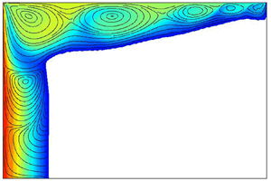
3.2. Oscillatory flow regime: the hydrothermal travelling wave
In figure 6, the evolution of the PCM phase change in a  $\varGamma = 12$ container subjected to a (large)
  $Ma = 186\,224$ (
 ${Ste} = 0.271$,
  ${\rm \Delta} T = 30$ K) is illustrated through selected snapshots. The colour map shows the temperature field between
  $\varTheta = 0$ (
 $T = T_M$, dark blue) and
  $\varTheta = 1$ (
 $T = T_M + 30$ K, dark red), with flow streamlines (black solid lines) and the
  $\varTheta = 0.5$ isotherm (white line) superimposed.

Figure 6. Snapshots (times indicated) showing the evolution of the PCM melting for  $\varGamma = 12$ (
 $H = 1.875$ mm,
  $L = 22.5$ mm) and a (large) applied
  $Ma = 186\,224$ (
 ${Ste} = 0.271$,
  ${\rm \Delta} T = 30$ K). The colour map shows the temperature field with flow streamlines (black solid lines) and the
  $\varTheta = 0.5$ isotherm (white line) superimposed. The solid volume is melted completely by
  $\tau _{melt} = 0.0870$ (510 s). During the process, the thermocapillary flow in the liquid phase (coloured) shows the hydrothermal travelling wave (HTW) oscillatory mode, characterised by the cyclic creation of vortices at the cold boundary
  $\varTheta = 0$ (i.e. at the solid/liquid interface or the cold wall) that travel towards the hot wall. The intensity of the travelling vortices decays progressively as they penetrate inwards. In the vicinity of the hot boundary, the travelling velocity decreases and the flow structure remains essentially standing.
At the very beginning of the phase-change process, heat transport is dominated by thermal diffusion. As soon as the solid/liquid front separates enough from the hot boundary, the thermocapillary effect drives convection near the free surface, as in figure 4. In this case, however, the local melting near the surface is fast enough that two different regions can already be distinguished in the liquid at  $\tau = 0.0034$: a thermocapillary-dominated region in the vicinity of the free surface, and a conductive-dominated region near the bottom wall. Despite the shorter time, the streamlines already indicate a flow structure of similar nature to that of the SMC discussed above, with three vortices spanning the liquid domain.
As time passes, the thin thermocapillary layer grows thicker until it spans the complete cell height, while the solid/liquid front advances through the cell, as shown at  $\tau = 0.0171$. From this time onwards, the solid/liquid interface maintains a similar overall shape, with approximately the same inclination (greater than that observed with smaller
  $Ma$), until reaching the cold endwall. During this transient, the existing SMC flow develops an increasing number of vortices, whose location along the container length is often nearly steady. At some instant, however, this underlying structure begins to oscillate, producing a hydrothermal travelling wave (HTW). With this applied
  $Ma$, the solid volume is completely melted by
  $\tau _{melt} = 0.0870$ (510 s).
The HTW is characterised by the cyclic creation of vortices at the cold boundary where  $\varTheta = 0$ (i.e. at the solid/liquid interface or the cold wall) that travel towards the hot wall. The intensity of the travelling motion decays as they move inwards. In the vicinity of the hot boundary, the flow structure is essentially standing. Part of this can be seen in the last three snapshots of figure 6 at
  $\tau = 0.0341, 0.0683, 0.1024$. The instability mechanism responsible for generating HTWs in high-
 $Pr$ liquids was discussed by Smith (Reference Smith1986), and shown to involve a (cyclic) energy transfer from the base flow to the temperature disturbance, and vice versa; hot perturbations at the interface are cooled by an upflow from underneath and, conversely, cold perturbations are warmed by an associated downflow.
In order to understand the different features of the HTW mode, temperature profiles are measured at selected locations along the cell length at  $\hat {y} = (2/3)\varGamma ^{-1}$ as illustrated in figure 7. In figure 7(a), temperature profiles are shown at three points
  $\hat {x} = \varGamma ^{-1}$ (black),
  $1/2$ (dark grey) and
  $1-\varGamma ^{-1}$ (light grey, labelled in the figure). By comparing with figure 5, the oscillatory nature of the thermocapillary flow is evident. Furthermore, two relevant times, indicated by vertical lines, can be inferred: the appearance of the HTW mode at
  $\tau _{osc}$, revealed by the signal oscillation; and the completion of melting at
  $\tau _{melt}$, revealed by the approach to a final HTW oscillatory mode solution.

Figure 7. Time evolutions of the dimensionless temperature  $\varTheta$ at
  $Ma = 186\,224$ (
 $Ste = 0.271$,
  ${\rm \Delta} T = 30$ K, as in figure 6), where the oscillatory HTW is found. (a) Temperatures
  $\varTheta$ at three selected sounding points distributed along the cell length
  $\hat {x} = \varGamma ^{-1}$ (black),
  $1/2$ (dark grey) and
  $1-\varGamma ^{-1}$ (light grey, labelled in the figure) at fixed vertical position
  $\hat {y} = (2/3)\varGamma ^{-1}$. Two relevant times are indicated by vertical lines: appearance of the HTW
  $\tau _{osc}$, and melting completion
  $\tau _{melt}$. (b) Temperature deviation
  $\hat {\varTheta } = \varTheta - \langle \varTheta \rangle$ with respect to the average
  $\langle \varTheta \rangle$ at
  $\hat {x} = 1/2$ (solid line) and
  $1/2 \pm {\rm \Delta} \hat {x}, {\rm \Delta} \hat {x} \simeq 0.04$ (dashed and dashed-dotted), showing the travelling nature of the oscillatory HTW mode.
By themselves, the temperature signals of figure 7(a) do not demonstrate the travelling nature of the HTW mode. To show this, we calculate the temperature deviation  $\hat {\varTheta } = \varTheta - \langle \varTheta \rangle$ with respect to the temporal average
  $\langle \varTheta \rangle$ at
  $\hat {x} = 1/2$ (solid line) and two equidistant points
  $\hat {x} \pm {\rm \Delta} \hat {x}, {\rm \Delta} \hat {x} \simeq 0.04$ (dashed and dashed-dotted), shown in figure 7(b). The shifted times at which the maxima of the curves occur demonstrate that these waves travel from the cold to the hot side of the container. At the same time, the fact that the peaks are not exactly at the same value shows that they are not purely travelling but include some degree of time-independent spatial modulation as well (i.e. a standing or pulsating component).
A more detailed look at the HTW mode is provided by figure 8(a–f), which shows six snapshots (approximately) equally distributed in time over one oscillation period of the temperature deviation field  $\hat {\varTheta }$ (left) and associated flow streamlines (right). The temperature deviation shows the motion of (cold and hot) perturbations from the cold side and how they vanish as they approach the hot boundary. The streamlines, on the other hand, reveal not only the motion of the vortices from the cold side, but also a certain degree of pulsating motion of the velocity field near the hot side, where the oscillatory mode becomes more of a standing wave. The wavenumber is estimated to be
  $kH \simeq 2$, consistent with the work of Smith & Davis (Reference Smith and Davis1983), which predicted
  $kH \rightarrow 2.47$ in the limit of
  $Pr \rightarrow \infty$. The simulations here capture the essentially two-dimensional behaviour of the HTW instability anticipated by these authors, who predicted a (small) propagation angle of 7.9
 $^{\circ }$ in the high-
 $Pr$ limit.

Figure 8. The HTW found at  $Ma = 186\,224$ (
 $Ste = 0.271$,
  ${\rm \Delta} T = 30$ K). (a–f) Temperature deviation
  $\hat {\varTheta }$ (left panels) and flow streamlines (right panels) at equally spaced times over (approximately) one oscillation period; the time increment between panels is
  ${\rm \Delta} \tau \simeq 1.7 \times 10^{-4}$ (1 s). (g) Time evolution of temperature deviation
  $\hat {\varTheta }$ at the horizontal line
  $\hat {y} = (2/3)\varGamma ^{-1}$ (indicated in panel (f)) for several oscillation periods. The colour map scale given in (g) is preserved between panels.
The evolution of the temperature field  $\hat {\varTheta }$ along
  $\hat {y} = (2/3)\varGamma ^{-1}$ (indicated in 8f by the solid horizontal line) is shown in figure 8(g) over many oscillation periods. The travelling nature of the wave is clear. Furthermore, its mean velocity can be estimated by the slope of the maxima (or minima) in the space–time plot. A slight change in the slope of these maximal (or minimal) curves can be discerned from
  $\hat {x} = 1$ (cold wall) to 0 (hot wall) as the travelling wave becomes increasingly more like a standing wave near the hot side.
It is informative to look at the characteristic frequency of the HTW obtained from a fast Fourier transform (FFT). In figure 9, (normalised) spectrograms calculated from the temperature deviation  $\hat {\varTheta }$ at
  $(\hat {x}, \hat {y}) = (1/2, (2/3)\varGamma ^{-1})$ are shown for three different applied Marangoni numbers: (a)
  $Ma = 108\,630$, (b) 124 149 and (c) 186 224, corresponding to
  ${Ste} = 0.158$, 0.180 and 0.271 and
  ${\rm \Delta} T = 17.5$, 20 and 30 K, respectively.

Figure 9. Spectrogram of the temperature deviation  $\hat {\varTheta } = \varTheta - \langle \varTheta \rangle$ (
 $\langle \varTheta \rangle$ is the time average) measured at
  $(\hat {x}, \hat {y}) = (1/2, (2/3)\varGamma ^{-1})$ for increasing Marangoni numbers in the HTW regime: (a)
  $Ma = 108\,630$, (b) 124 149 and (c) 186 224. These values correspond to
  ${Ste} = 0.158$, 0.180 and 0.271 and
  ${\rm \Delta} T = 17.5$, 20 and 30 K. Frequencies are non-dimensionalised with the thermal diffusion time scale
  $(L^2/\alpha )$.
In general, the spectral content of the HTW mode increases with the applied  $Ma$. At (moderate)
  $Ma$ (9a), there is a single dominant spectral peak at the natural frequency of the oscillation,
  $\varOmega = f(L^2/\alpha ) \simeq 1.17 \times 10^3$ (
  $f \simeq 0.2$ Hz, with units restored). Increasing the applied
  $Ma$ does not substantially modify this frequency but does lead to more harmonic content in the signal. At
  $Ma = 124\,149$ (9b), the frequencies
  $\varOmega \simeq 1.17 \times 10^3$ and
  $2.34 \times 10^3$ (
  $f \simeq 0.2, 0.4$ Hz) are both relevant, while in 9(c) at
  $Ma = 186\,224$, the third harmonic is significant as well. It can be expected that, for high enough
  $Ma$, chaotic thermocapillary flow can be found with a much broader spectral response. Here, the distinction mentioned above between the time scales of the melting process and the oscillatory modes is evident. At
  $Ma = 186\,224$, for example, the (dimensional) oscillation period is of the order of 5 s, while it takes 510 s to observe the complete solid–liquid phase transition, showing a ratio of roughly 0.01.
The formation and propagation of HTWs during solidification in large containers were recently analysed by Lappa (Reference Lappa2018). The solidification was controlled by prescribing temperature ramps at the cold side of the container and the evolution of the oscillatory mode was traced during the process. Spectral analysis revealed the presence of a transition from the initial single-frequency HTW solution to a three-frequency mode with: (i) a first frequency similar to that of the initial HTW, (ii) a second frequency related to the temperature ramping, and (iii) a third frequency that was the difference of the other two. Our results have a simpler spectral profile since constant temperatures are applied at the boundaries. The spectra observed here, with the basic frequency of oscillation and higher harmonics, are more similar to the results of Shevtsova et al. (Reference Shevtsova, Nepomnyashchy and Legros2003).
Finally, we plot the spectrogram (calculated at the completion of the phase change) against the applied  $Ma$ in figure 10(a). The increase in spectral content with applied
  $Ma$ is apparent, while at lower values of
  $Ma$, there is no oscillatory behaviour at all. The vertical lines in 10(a), labelled as ‘a’, ‘b’ and ‘c’, refer to the
  $Ma$ values of figure 9.

Figure 10. (a) Successive spectrograms of the temperature deviation  $\hat {\varTheta }$ measured at
  $(\hat {x}, \hat {y}) = (1/2, (2/3)\varGamma ^{-1})$ at the completion of melting over a wide range of
  $Ma \in [62\,075, 248\,298]$ (
 ${\rm \Delta} T \in [10, 40]$ K). The black vertical lines indicate the
  $Ma$ of associated spectrograms shown in figure 9. (b) Contribution of the oscillatory HTW mode to the phase change
  $\mathcal {C}_{HTW}$ (i.e. percentage of the total melting time with HTW) over the same range of
  $Ma$. Simulations are denoted by markers, which are colour-coded according to whether the thermocapillary flow is steady (black) or that of the HTW mode (red). The fit (dashed line) for these discrete measurements provides an estimate of the critical
  $Ma$ (green marker) for the HTW mode, which is
  $Ma_{cr} = 97\,660$, corresponding to a
  $Ste_{cr} = 0.133$ and
  ${\rm \Delta} T_{cr} = 15.73$ K. This threshold is labelled and indicated by the green vertical line in panel (a).
3.3. Onset of oscillatory convection
From the previous discussion, it is clear that there is a critical Marangoni number  $Ma_{cr}$ for the appearance of the HTW mode. However, in contrast to thermocapillary flow in a pure liquid phase, where the supercritical nature of the instability allows an accurate estimate of the threshold from the variation of the oscillation amplitude (see e.g. Preisser, Schwabe & Scharmann Reference Preisser, Schwabe and Scharmann1983), the gradual change of liquid volume due to the phase-change process complicates this approach.
Generally, temperature measurements are as shown in figure 7, with long transient times needed to reach a quasi-steady amplitude affected primarily by the slower evolution of the solid/liquid front during melting. To get around this problem, we propose to use the thermocapillary contribution of the HTW mode  $\mathcal {C}_{HTW}$, defined as the total time that the oscillatory motion exists relative to the total melting time, which usually simplifies to
 \begin{equation} \mathcal{C}_{HTW} = \left(1- \frac{\tau_{osc}}{\tau_{melt}} \right) \times 100\ (\textrm{in}\,\%). \end{equation}
 In figure 10(b), the calculated  $\mathcal {C}_{HTW}$ values are plotted against the associated
  $Ma$. The markers denoting simulations are colour-coded according to whether the flow regime is steady (black) or that of the HTW mode (red). A fit of these values (dashed line) provides an estimate of the critical
  $Ma$ (in green, also marked in 10(a) by a vertical green line) for the HTW mode. For
  $\varGamma = 12$, it is found to be
 \begin{equation} Ma_{cr} = 97 \,660, \end{equation}
corresponding to  $Ste_{cr} = 0.133$ and a critical temperature difference
  ${\rm \Delta} T_{cr} = 15.73$ K.
4. Thermocapillary flows during the phase change in small-aspect-ratio containers
The phase change is now analysed in small-aspect-ratio containers. Again, qualitatively similar results are obtained for  $\varGamma \lessapprox 4$. We select
  $\varGamma = 2.25$ as a representative case to illustrate the different dynamics that can occur during the phase transition depending on the applied
  $Ma$. As for large-aspect-ratio containers, the associated thermocapillary flow can be either steady or oscillatory, with each treated in separate sections below.
4.1. Steady flow regime: from small-scale SMC states to large-scale steady vortical structures
In figure 11, four snapshots show the time evolution of the PCM phase change for  $\varGamma = 2.25$ (
 $H = 10$ mm,
  $L = 22.5$ mm) and a (moderate) applied
  $Ma = 62\,075$ (
 ${Ste} = 0.090$,
  ${\rm \Delta} T = 10$ K). The colour map shows the temperature field between
  $\varTheta = 0$ (
 $T = T_M$, dark blue) and
  $\varTheta = 1$ (
 $T = T_M + 10$ K, dark red), with flow streamlines (black solid lines) superimposed.

Figure 11. Snapshots (times indicated) showing the evolution of the PCM melting for  $\varGamma = 2.25$ (
 $H = 10$ mm,
  $L = 22.5$ mm) and a (moderate) applied
  $Ma = 62\,075$ (
 ${Ste} = 0.090$,
  ${\rm \Delta} T = 10$ K). The colour map shows the temperature field with flow streamlines (black solid lines) superimposed. The solid volume is melted completely by
  $\tau _{melt} = 1.5677$ (9185 s). During the process, the thermocapillary flow in the liquid phase (coloured) exhibits a transition from a small-scale SMC to a large-scale steady vortical structure (SVS). As the phase change progresses, an initial series of vortices along the thin liquid layer near the free surface (where the effective local aspect ratio is large) transforms into an SVS flow with one strong vortex near the hot side and a weaker one near the cold side. The horizontal line at
  $\tau = 0.1195$ indicates the selected cut
  $\hat {y} = (9/10)\varGamma ^{-1}$ used for the temperature profiles shown in figure 12.
At the early times of the phase change, heat transport is dominated by thermal diffusion. As soon as the solid/liquid front separates enough from the hot boundary, the thermocapillary effect drives convection in an initially thin region (compared with  $H$) near the free surface. The melting process is locally enhanced, which accelerates the progression of the solid/liquid front near the liquid–air boundary, as shown at
  $\tau = 0.1195$. The effective aspect ratio within this layer is generally larger than
  $\varGamma$, and thus a flow structure reminiscent of a small-scale SMC is observed within the layer; this solution is typical of larger-aspect-ratio containers (see § 3, for details). The streamlines included at
  $\tau = 0.3415$ illustrate this structure, which is characterised by a series of vortices that spread from the hot to the cold boundary. During this time, the cold boundary is essentially determined by the advancing solid/liquid front. The liquid near the bottom wall, on the other hand, indicates a phase change driven mainly by thermal diffusion. This is evident from the local temperature field, which shows (vertical) isotherms parallel to the lateral endwalls.
As this layer evolves, the solid/liquid front reaches the cold lateral boundary and the liquid phase depth near this boundary increases with time. This means that the effective aspect ratio for the thermocapillary flow slowly decreases and the vortices move towards the cold endwall. At some point, the smaller vortex near this boundary is absorbed by its neighbour, which reduces the number of vortices by one. This process is repeated until a final configuration of two vortices is reached, as shown at  $\tau = 1.0241$. The vortical structure selected in the final configuration depends on the cell aspect ratio (Bergeon et al. Reference Bergeon, Henry, Benhadid and Tuckerman1998); the limiting case of one single vortex would be observed for reduced aspect ratios (Zebib et al. Reference Zebib, Homsy and Meiburg1985; Carpenter & Homsy Reference Carpenter and Homsy1990).
At the completion of melting, which occurs by  $\tau = 1.5677$ (9185 s), the flow contains two vortices of different intensity, similar to the structure discussed by Peltier & Biringen (Reference Peltier and Biringen1993), with the main vortex biased towards the hot wall, consistent as well with Carpenter & Homsy (Reference Carpenter and Homsy1990). For this applied
  $Ma$, the flow remains steady and temperature oscillations are not observed. This is demonstrated in figure 12, where the time evolution of the temperature profile along the
  $\hat {y} = (9/10)\varGamma ^{-1}$ line (marked by a solid line at
  $\tau = 0.1195$ in figure 11) is shown.

Figure 12. Evolution of the temperature profile at  $\hat {y} = (9/10)\varGamma ^{-1}$ for the complete solid–liquid transition illustrated in figure 11. The colour map shows the temperature field and demonstrates the steady nature of the vortical structure over the complete melting process.
Not only is the steady nature of the melting process clear from the temperature field, but the quasi-steady evolution of the flow structure is also evident. The initial vortex that is (nearly) centred along this line progressively occupies the left half of the cell, while the smaller vortices that form along with the SMC slowly disappear near the cold boundary and are absorbed by their neighbours. In short, the thermocapillary flow evolves from a small-scale (compared with container dimensions) SMC to a large-scale steady vortical structure (SVS).
Finally, as for  $\varGamma \gg 1$, the steady nature of this thermocapillary flow becomes unstable at a certain
  $Ma$, where it gives way to an oscillatory mode. The features of this mode are presented and analysed below.
4.2. Oscillatory flow regime: the oscillatory standing wave
In figure 13, snapshots at selected times show the evolution of the phase change for  $\varGamma = 2.25$ (
 $H = 10$ mm,
  $L = 22.5$ mm) and a (large) applied
  $Ma = 186\,224$ (
 ${Ste} = 0.271$,
  ${\rm \Delta} T = 30$ K). The colour map shows the temperature field between
  $\varTheta = 0$ (
 $T = T_M$, dark blue) and
  $\varTheta = 1$ (
 $T = T_M + 30$ K, dark red), with flow streamlines (black solid lines) superimposed.

Figure 13. Snapshots (times indicated) showing the evolution of the PCM melting for  $\varGamma = 2.25$ (
 $H = 10$ mm,
  $L = 22.5$ mm) and a (large) applied
  $Ma = 186\,224$ (
 ${Ste} = 0.271$,
  ${\rm \Delta} T = 30$ K). The colour map shows the temperature field with flow streamlines (black solid lines) superimposed. The solid is melted completely by
  $\tau _{melt} = 0.5461$ (3200 s). During the process, the thermocapillary flow in the liquid phase (coloured) is that of an oscillatory standing wave (OSW) mode, characterised by a periodic pulsation where the intensity of the two principal vortices cycles back and forth.
The progression of the phase change is fairly similar to that of § 4.1, with the total time of the melting reduced as expected for an applied  $Ma$ that is three times larger. The flow in the liquid initially shows two regions: the thermocapillary-dominated region near the free surface, and the thermal diffusion-dominated region near the bottom wall. As the applied
  $Ma$ is increased, the localised SMC contains four vortices (see the temperature field and streamlines at
  $\tau = 0.0512$), one more than the three vortices shown at
  $\tau = 0.3414$ in figure 11 for a similar solid/liquid interface location. As time passes, however, the associated thermocapillary flow does not have the simple structure of two asymmetric vortices but a more complex evolving flow structure, as illustrated at
  $\tau = 0.3414, 0.4694, 0.5632$.
To confirm the oscillatory (more generally, unsteady) nature of the flow, the temperature field (upper row) and the associated spectrograms (lower row) at different points of the container are shown in figure 14. For consistency with § 3, these measurement points are chosen along the line  $\hat {y} = (2/3)\varGamma ^{-1}$ at three different locations: (a)
  $\hat {x} = 1/8$ (black), (b)
  $1/2$ (dark grey) and (c)
  $7/8$ (light grey, labelled in the panels). Two important times are indicated by solid vertical lines: the appearance of the oscillatory standing wave (OSW) at
  $\tau _{osc}$ and
  $\tau _{melt}$.

Figure 14. Evolution of the dimensionless temperature  $\varTheta$ for
  $Ma = 186\,224$ (
 ${\rm \Delta} T = 30$ K, as in figure 13), where the OSW is found. In the upper row, temperatures are shown at (a)
  $\hat {x} = 1/8$ (black), (b)
  $1/2$ (dark grey) and (c)
  $7/8$ (light grey), labelled in the panels, with the fixed vertical position
  $\hat {y} = (2/3)\varGamma ^{-1}$. Two relevant times are indicated by vertical solid lines: appearance of the OSW
  $\tau _{osc}$, and end of melting
  $\tau _{melt}$, while dashed lines mark the selected times for the oscillation periods shown in figure 15 (labelled between rows). The lower row shows associated spectrograms for the temperature deviation
  $\hat {\varTheta } = \varTheta - \langle \varTheta \rangle$.
Aside from the oscillatory behaviour, which is evident in these profiles, there is a significant difference compared with the results at large aspect ratios that can be seen in the associated spectrograms. For  $\varGamma = 12$, the spectrograms of figure 9 show a single dominant frequency for the HTW mode that is nearly independent of the applied
  $Ma$ or the evolution of the solid/liquid front; this is consistent with the idea that it is the (nearly constant) cold boundary region that is selecting the HTW frequency. For the OSW mode in small-aspect-ratio containers, in contrast, there is a notable variation of the principal frequency over time and in space. This mode has more complicated spectral behaviour due to the interaction of the different regions near the free surface and near the bottom of the container and the progressive loss of vortices from the underlying SMC type of structure. The dominant (dimensionless) frequency changes substantially during the melting process, from
  $\varOmega \simeq 2.34 \times 10^3$ (
  $f \simeq 0.4$ Hz) at the appearance of oscillatory motion to
  $\varOmega \simeq 0.41 \times 10^3$ (
  $f \simeq 0.07$ Hz) when melting finishes. We note again that the time scale of the oscillatory flow, which ranges between 2 and 14 s, is substantially smaller compared with the melting time of 3200 s.
The spectral content of the temperature signals varies significantly along the length of the container too. When melting completes, the oscillations are relatively weak near the hot side, with stronger oscillations concentrated near the cold side. In fact, compared with figure 9(c), where the same  $Ma = 186\,224$ was applied, the spectral content of the signal is much richer here, with the dominant frequency of the OSW mode roughly half that of the HTW mode. They are clearly distinct instabilities.
This complex scenario can be better understood by focusing on selected oscillation periods throughout the melting process. In figure 15, equally distributed snapshots are shown during one period of oscillation centred at the times (a)  $\tau = 0.0512$ (300 s), (b) 0.1195 (700 s) and (c) 0.5632 (3300 s). The corresponding oscillation frequencies (periods are labelled in the panels) are
  $\varOmega \simeq 2.34 \times 10^3$,
  $1.93 \times 10^3$ and
  $0.41 \times 10^3$ (
  $f \simeq 0.4, 0.33, 0.07$ Hz), respectively.

Figure 15. Details of the OSW mode during the phase change in a container of  $\varGamma = 2.25$ subjected to
  $Ma = 186\,224$ (
 ${Ste} = 0.271$,
  ${\rm \Delta} T = 30$ K). Temperature fields are shown at selected times (equally spaced) over an oscillation period at (a)
  $\tau = 0.0512$ (300 s), (b) 0.1195 (700 s) and (c) 0.5632 (3300 s). Streamlines are superimposed in the final set of snapshots.
At  $\tau = 0.0512$, the oscillatory mode features five pulsating vortices that spread along the thin liquid layer near the interface. The progressive melting reduces the number of oscillating vortices in the structure and the associated frequency decreases gradually. At
  $\tau = 0.1195$, the mode is characterised by the pulsation of three vortices, whose effect on the solid/liquid front is evident in its curvature.
As time passes, this three-vortex structure is reduced to two asymmetric pulsating vortices. At this point, the cycle involves the generation of a counter-flow near the free surface, which is indicated by the appearance in the streamlines of a new vortex. The oscillatory motion observed at the completion of melting is analogous to the oscillatory mode described by Peltier & Biringen (Reference Peltier and Biringen1993).
The instability mechanism can be described following Peltier & Biringen (Reference Peltier and Biringen1993). The clockwise sense of rotation of the largest vortex allows a cool stream of liquid to be siphoned away from the cold boundary (either the solid/liquid front or the endwall) along the bottom of the container. Near the hot wall, this stream is redirected upwards, creating a cool tongue that interacts with the thermocapillary surface. The cool tongue creates a large thermal gradient near the hot wall that causes the primary convection cell to compress towards this boundary and strengthen (see first and second panels of figure 15c). In turn, the shear forces from this primary vortex near its cold side weaken, and a secondary vortex with the same sense of rotation appears. Between these, an additional tertiary vortex with the opposite sense of rotation appears, supported by the shear between the primary and secondary cells and the weak local temperature gradient of the interface (in an adverse sense with respect to the rotation of this cell; see third panel of figure 15c).
The primary and secondary vortices strengthen up to a certain point (fourth panel of figure 15c), where two different mechanisms come into play to recover the initial single cell structure. First, in the absence of sufficient reinforcement of liquid from the cold wall, the cool tongue near the hot wall warms up and its effect on the surface diminishes; this retraction of the cool finger can be seen between the third and fifth panels in figure 15(c). Secondly, the increased strength of the primary vortex draws hot liquid from the hot wall. The secondary vortex, on the other hand, draws cold fluid from the cold boundary and ejects it upwards towards the thermocapillary surface (see the fourth snapshot in figure 15c). The surface is thus cooled locally, which reduces the driving force that maintains the secondary cell. Through this process, the secondary cell brings about its own extinction, which favours the expansion of the primary vortex and a return to the original state.
This oscillation relies on the interaction between the sensitivity of the surface to the cooling effect provided by the cold tongue and the extent to which the cool stream that is expelled from the cold boundary can influence the cold tongue. It thus makes sense that the oscillation period increases as the driving force (via the cold tongue) is effectively reduced with increasing vortex size, which explains the general observation in the spectrograms of decreasing frequencies during the phase change.
One may also expect that this oscillation can disappear during the melting process if the (nearly) horizontal solid/liquid front near the cold side moves down far enough in the cell; in other words, when the primary vortex is large enough for its influence on the thermocapillary surface to diminish. We posit that this transition from OSW to SVS was observed in the container of  $\varGamma = 1.5$ (
 $H = 15$ mm) in the present simulations, with further details given below.
4.3. Onset of oscillatory convection
Again, it is clear from these results that there is a  $Ma_{cr}$ for the appearance of the OSW mode. As in § 3.3, we locate this transition by using the thermocapillary contribution of the OSW mode
  $\mathcal {C}_{OSW}$, defined as the total time that the oscillatory motion exists relative to the total melting time, which usually simplifies to
 \begin{equation} \mathcal{C}_{OSW} = \left(1- \frac{\tau_{osc}}{\tau_{melt}} \right) \times 100\ (\textrm{in}\,\%). \end{equation}
 In figure 16,  $\mathcal {C}_{OSW}$ is plotted against
  $Ma$. Simulations are colour-coded according to whether the flow is steady (black) or that of the OSW mode (blue). The fit (dashed line) to these measured values provides an estimate of the critical value (in green) for the OSW mode. For
  $\varGamma = 2.25$, it is found to be
 \begin{equation} Ma_{cr} = 68 \,852, \end{equation}
corresponding to  $Ste_{cr} = 0.100$ and a critical temperature difference of
  ${\rm \Delta} T_{cr} = 11.09$ K.

Figure 16. Contribution of the OSW mode to the phase change  $\mathcal {C}_{OSW}$ (i.e. percentage of the total melting time) for a wide range of
  $Ma \in [31\,038, 248\,298]$ (
 ${\rm \Delta} T \in [5, 40]$ K). Simulations are denoted by markers, which are colour-coded according to whether the thermocapillary flow is steady (black) or that of the OSW mode (blue). The fit (dashed line) for these measurements provides an estimate of the critical
  $Ma$ (green marker) for the OSW mode, which is
  $Ma_{cr} = 68\,852$, corresponding to
  $Ste_{cr} = 0.100$ and
  ${\rm \Delta} T_{cr} = 11.09$ K.
Thus, not only does the evolution of the thermocapillary flow depend on the aspect ratio, but the onset values are different. We now discuss the combined effect of  $Ma$ and
  $\varGamma$.
5. Overview of the thermocapillary flow regimes during the PCM phase change
The analyses of §§ 3 and 4 have examined the different thermocapillary flows that are observed in the liquid phase of a PCM with a free surface during its melting process in microgravity.
In large-aspect-ratio containers, the thermocapillary flow at small  $Ma$ is initially characterised by a large vortex that spans the liquid domain, with the typical SRF structure (Sen & Davis Reference Sen and Davis1982; Strani et al. Reference Strani, Piva and Graziani1983). Increasing
  $Ma$ destabilises this large vortex to a series of vortices appearing in an SMC. By increasing
  $Ma$ even more, this SMC undergoes a transition to a periodic HTW, which is characterised by the cyclic creation of vortices near the cold side that travel inwards to the hot side. The time at which this HTW mode first appears during the phase change depends on the applied
  $Ma$. During the time these travelling waves exist, they affect heat transport and contribute to the phase-change process. By calculating their contribution to the phase change, one can estimate the critical
  $Ma$.
$Ma$.
In small-aspect-ratio containers, on the other hand, the thermocapillary flow at small to moderate  $Ma$ is initially characterised by the transition from a small-scale SMC, located in a thin layer near the free surface where the local aspect ratio is larger than
  $\varGamma$, to a large-scale SVS. Upon increasing
  $Ma$, a complex oscillatory mode appears, characterised by the pulsation of the underlying vortical structure. In fact, as this structure evolves during the phase change by reducing the number of its vortices, the frequency of the oscillation also decreases. We refer to this mode as OSW, which is qualitatively different than the HTW. Again, the associated critical
  $Ma$ can be estimated by plotting the percentage of time that it exists relative to the total melting time.
To complete these analyses, sets of simulations were performed over a wide range of  $Ma$
$Ma$  $\in (6000, 248\,298]$ (
 ${\rm \Delta} T \in (1, 40]$ K) in rectangular cells of ten different
  $\varGamma$, covering the interval
  $\varGamma \in [1.5, 22.8]$, which includes small, intermediate and large values. Figure 17 summarises the different thermocapillary flow regimes observed during the phase change in terms of (a)
  $Ma$ and
  $\varGamma$ and (b)
  ${\rm \Delta} T$ and
  $H$ (for a fixed
  $L = 22.5$ mm). The simulation results are colour-coded according to whether the observed flow was steady (black), an HTW mode (red) or an OSW mode (blue). The critical boundary for oscillatory flow is marked by a solid green line.

Figure 17. Overview of the type of thermocapillary flow observed during the PCM phase change as a function of (a)  $Ma$ and
  $\varGamma$, and (b)
  ${\rm \Delta} T$ (in K) and
  $H$ (in mm); recall that
  $L = 22.5$ mm. Distinct modes are marked in different colours: steady flow (black), HTW (red) and OSW (blue). The critical boundary for oscillatory flow is marked by a solid green line. Note the logarithmic scale used in the vertical axis of panel (a).
Figure 17 illustrates the distinction between large- and small-aspect-ratio containers already discussed, and suggests how the thermocapillary flow during the phase change changes between them. In the transition regime, simulations were performed with a rectangular cell of  $\varGamma = 5.29$ (
 $H = 4.25$ mm,
  $L = 22.5$ mm). At low
  $Ma$, the flow was steady and a small-scale SMC appears. Upon increasing
  $Ma$, this vortical structure becomes unstable to the HTW mode. During the phase change, HTWs usually appear for a limited duration during the melting and disappear again so that the final thermocapillary flow is an SVS. At certain
  $Ma$, the evolution of the flow becomes completely steady, with the initial small-scale SMC developing directly into a large-scale SVS. This steady regime, however, persists only over a small range of
  $Ma$ and becomes unstable to the OSW mode at larger values.
An explanation for this transition regime can be taken from the work of Peltier & Biringen (Reference Peltier and Biringen1993), where thermocapillary flows were analysed in rectangular two-dimensional domains with aspect ratios between 2.3 and 3.8 for a  $Pr = 7.78$ fluid. Figure 3 of that reference is especially relevant, where the instability map in terms of
  $\varGamma$ and
  $Ma$ is presented. Regions showing a double-valued critical onset (zero amplitude curves) are obtained so that, for fixed
  $\varGamma$, transitions from steady to oscillatory and back to steady solutions are observed with increasing
  $Ma$ (or vice versa).
In the present work, since the melting front constitutes a moving boundary for the liquid phase, this transition can be understood as a change in effective aspect ratio of the liquid. We note that, regardless of  $\varGamma$, the initial effective aspect ratio tends to zero. In large containers, this effective aspect ratio rapidly takes a large value, and thus the preferred flow is the HTW mode. In small-aspect-ratio containers, the effective ratio is more limited and takes a maximum value where we consistently observe the selection of SMC states, then later decreases towards
  $\varGamma$.
For intermediate containers, the effective ratio evolves in a more complex manner, potentially exhibiting various maxima and minima during the process. One may imagine that the instantaneous value of the effective aspect ratio selects the preferred oscillatory mode (either OSW or HTW), with the stability of the system changing as it passes a critical value. This picture is consistent with the results obtained for  $\varGamma = 5.29$. At low
  $Ma$, the relative evolution between the conductive-dominated and thermocapillary-dominated regions of the domain selects the SMC first. This steady structure is later destabilised to the HTW mode, which persists within a finite range of
  $Ma$. For increasing values, a last transition from an SVS to an OSW mode is observed, again as the effective aspect ratio transitions across the corresponding critical values.
In the smallest aspect ratio considered,  $\varGamma = 1.5$, the thermocapillary flow also undergoes two transitions from steady to oscillatory, and from oscillatory back to steady. This was anticipated in § 4.2 when discussing the sensitivity of the OSW mode to the influence of the cold tongue on the thermocapillary surface, and can be explained in a similar way. In this case, the effective aspect ratio crosses the same (OSW) instability boundary twice.
Finally, it is worth clarifying that we have referred to any phase-change transition as ‘oscillatory’ if it involved oscillatory flows at any lapse during melting. This is also behind the term ‘oscillatory mode contribution’ to the phase change and is consistent with the overall enhancement of thermocapillary convection on heat transport that was demonstrated by the works of Ezquerro et al. (Reference Ezquerro, Bello, Salgado Sánchez, Laveron-Simavilla and Lapuerta2019, Reference Ezquerro, Salgado Sánchez, Bello, Rodriguez, Lapuerta and Laveron-Simavilla2020) and Salgado Sánchez et al. (Reference Salgado Sánchez, Ezquerro, Porter, Fernandez and Tinao2020b), and which is apparent in the present results.
6. Conclusions
A detailed numerical investigation of thermocapillary flows during the melting of phase-change materials in microgravity is presented.
The phase-change transition is modelled using an enthalpy–porosity based formulation of the Navier–Stokes equations (Voller et al. Reference Voller, Cross and Markatos1987), and analysed for the high-Prandtl-number organic paraffin n-octadecane ( $Pr = 52.53$) due to its relevance to recent microgravity experiments (Ezquerro et al. Reference Ezquerro, Bello, Salgado Sánchez, Laveron-Simavilla and Lapuerta2019, Reference Ezquerro, Salgado Sánchez, Bello, Rodriguez, Lapuerta and Laveron-Simavilla2020; Salgado Sánchez et al. Reference Salgado Sánchez, Ezquerro, Porter, Fernandez and Tinao2020b). The PCM is enclosed in a rectangular (two-dimensional) container with isothermal conditions along the left and right lateral walls. The progressive evolution of the solid/liquid front during the melting process leaves a free surface along which a temperature variation exists. The associated gradient of surface tension drives thermocapillary convection in the liquid phase. In this paper, the different thermocapillary flows found during the melting process are analysed, following the usual division according to aspect ratio.
In large- $\varGamma$ containers, analysed in § 3, the thermocapillary flow at small
  $Ma$ is initially characterised by a large vortex that spans the liquid domain, with the classical features of a steady return flow (SRF). Increasing
  $Ma$ destabilises this large vortex, which is replaced by a series of vortices in a steady multicellular structure (SMC). By further increasing
  $Ma$, this SMC state undergoes a transition to a hydrothermal travelling wave (HTW), which is characterised by the periodic creation of vortices near the cold side that travel inwards to the hot side. The appearance of this HTW mode during the phase change depends on the applied
  $Ma$, and these travelling waves exist during a certain portion of the total melting time, during which they contribute to the phase-change process. By calculating this contribution, one can estimate the critical
  $Ma$ for the appearance of the HTW mode.
In small-aspect-ratio containers, analysed in § 4, the thermocapillary flow at small to moderate  $Ma$ is initially characterised by the transition from a small-scale SMC state, which develops in a thin layer near the free surface where the local aspect ratio is larger than
  $\varGamma$, to a large-scale steady vortical structure (SVS). By increasing
  $Ma$, a complex oscillatory mode appears, which is characterised by the pulsation of the underlying vortical structure. As this structure evolves during the phase change by reducing the number of its vortices, the natural frequency of the oscillation also decreases. We refer to this state as an oscillatory standing wave (OSW) mode due to its clear qualitative differences with respect to the HTW. Again, plotting the associated oscillatory contribution provides an estimate of the critical
  $Ma$ for the OSW mode.
Finally, in § 5, results are summarised in terms of  $Ma$ and
  $\varGamma$, delineating the different thermocapillary flow regimes observed during the phase-change process, and establishing the stability boundaries for the HTW and OSW modes. The transition regime separating them is also analysed, with the choice of
  $\varGamma \simeq 5.3$. At low
  $Ma$, the flow is steady, with the appearance of a small-scale SMC. With increasing
  $Ma$, this vortical structure becomes unstable to the HTW mode. During the phase change, HTW modes typically appear for a limited portion of the melting time and disappear again prior to the emergence of the final thermocapillary flow state, which is again an SVS mode. At a certain
  $Ma$, the phase change becomes fully (quasi-)steady with the initial small-scale SMC developing directly into a large-scale SVS state. This behaviour occurs only over a small range of
  $Ma$ and becomes unstable to the OSW mode at larger values.
Several aspects of the results described here suggest themselves for further investigation, an effort that will be undertaken separately. First, further simulations will be performed to investigate the transition region in more detail and accurately locate the instability boundaries, and to determine if a suitable definition of the effective (transient) aspect ratio for the liquid phase during the melting process can be used to understand them. On the experimental side, we are currently developing a ground-based set-up that will allow us to make systematic measurements of the phase-change process in different organic paraffins, including n-octadecane, under the presence of a controlled thermocapillary interface. It is expected that these experiments will confirm some of the behaviour found in the simulations presented here and allow for a refinement of the model. An extension of the numerical model to three dimensions is also planned. Finally, these investigations would most benefit from a comparison with (future) microgravity experiments covering the entire PCM melting cycle. Such experiments could confirm the existence of the thermocapillary flows described here and, in particular, investigate the transition between HTW and OSW modes.
Acknowledgements
This work was supported by the Spanish User Support and Operations Centre (E-USOC) and the Escuela Técnica Superior de Ingeniería Aeronáutica y del Espacio at the Universidad Politécnica de Madrid. We thank the research group of Ciencias y Operaciones Aeroespaciales for their invaluable efforts and, in particular, Professor J. Porter for helpful discussions and the English revision of the manuscript.
Declaration of interests
The authors report no conflict of interest.


