2. Experiment

All measurements were conducted in three rectangular HC samples with the same aspect ratio $\varGamma = L : W : H = 10:1:1$, filled with water. The samples have different lengths ($L = 0.5$, $1.0$ and 2.0 m) in order to extend the accessible Rayleigh number $Ra \equiv \alpha g \varDelta L^{3}/(\nu \kappa )$ range. Here $\alpha$, $\nu$ and $\kappa$ denote, respectively, the isobaric thermal expansion coefficient, the kinematic viscosity and the thermal diffusivity of the fluid; $g$ is the gravitational acceleration and $\varDelta = T_h - T_c$ is the temperature difference between the heating ($T_h$) and cooling ($T_c$) plates. As shown in figure 1, both plates are squares with width $W$ and a thickness of $5$ cm, and they were placed on the sample bottom. They were made of copper and their surfaces were electroplated with a thin layer of nickel. The remaining parts of the samples were made of acrylic of $30$ mm in thickness for good thermal insulation. In experiment, the samples were carefully levelled relative to gravity to within $10^{-3}\ \textrm {rad}$.

Figure 1. Schematic diagram of HC sample with the aspect ratio $L:W:H = 10:1:1$. Cooling plate (blue part) and heating plate (red part) are squares with the width $W$. Four vertical dashed lines indicate the locations of measured temperature profiles at $x/L = 0.01$, $0.05$, $0.95$ and $0.99$ in the plane of $y/W = 0.5$. Also sketched are profiles of the large-scale horizontal flow and vertical mean temperature above the two plates.

The temperature difference $\varDelta$ was set in the range of $10\ \textrm {K} \leq \varDelta \leq 35\ \textrm {K}$ in three samples, and the corresponding $Ra$ range is $2\times 10^{10} \lesssim Ra \lesssim 9 \times 10^{12}$. The data show that the HC bulk temperature $T_o = T_c + \chi \varDelta$ with the obtained $\chi$ from $0.81$ to $0.89$ over the $Ra$ range, while $\chi = 0.5$ for RBC under the Boussinesq approximation. As a result, the Prandtl number $Pr\equiv \nu /\kappa$, which is evaluated at $T_o$, varies from $3.9$ to $6.5$ accordingly. For $Pr \gtrsim 1$ the global heat transport in laminar HC, as expressed by the Nusselt number $Nu \equiv qL/(k\varDelta )$ ($q$ is the heat flux through the heated plate and $k$ is the fluid thermal conductivity), is independent of $Pr$, while for small $Pr$, it scales as $Nu \sim Pr^{1/10}$ (Shishkina et al. Reference Shishkina, Grossmann and Lohse2016; Shishkina & Wagner Reference Shishkina and Wagner2016). Therefore, the variations of $Pr$ in the experiment might lead, at most, to a 5 % error in the $Nu$ data, which would not affect much the results on the temperature profiles. However, in order to eliminate this weak $Pr$ dependence, we selected the measurements at $Pr \simeq 6$ only.

The procedures of temperature control and measurements in HC are similar to those in RBC described previously by He & Tong (Reference He and Tong2009). We used the calibrated thermistors (Honeywell 112-104KAJ-B01) with a diameter of 1.13 mm and accuracy of 5 mK to measure the temperature on the plates. Two thermistors were installed in each plate at a distance of 5 mm away from the top surface to ensure good thermal homogeneity. The entire HC sample was thermally insulated by several layers of rubber shields and was placed inside a temperature-controlled box. The temperature in the box was regulated at $T_o$ with a long-time stability of ${\pm }0.1\ \textrm {K}$, in order to prevent heat exchanges between the convection flow and the surroundings.

We used smaller glass-encapsulated thermistors (Honeywell 111-104HAK-H01) to measure time-dependent temperature profiles in the vertical $z$-direction, at four horizontal locations $x/L$ above both plates, as sketched in figure 1. These thermistors have a diameter of 0.36 mm and were calibrated with 5 mK precision. We used a double-hole ceramic tube with a diameter of 0.8 mm to assemble one thermistor, and mount it on a vertical translational stage with the spatial resolution of $10\ \mathrm {\mu }\textrm {m}$. Details about the temperature calibration and measurements were reported before by Wang et al. (Reference Wang, Xu, He, Yik, Wang, Schumacher and Tong2018). At each measuring location along a profile, we took 2 h-long real-time data at the rate of 15 Hz.

3. Theoretical model for laminar thermal BL in HC

For all $Ra$ in the experiment, the maximal normalized root-mean-square (r.m.s.) temperature $\sigma _{T}/\varDelta$ above the cooling plate is $0.005$. In comparison, the maximal $\sigma _{T}/\varDelta$ near the thermal BL in RBC for $Ra \simeq 10^{9}$ is approximately 0.08 (Shishkina & Thess Reference Shishkina and Thess2009; He, Ching & Tong Reference He, Ching and Tong2011). Recent DNS results also showed that both the kinetic energy and dissipation rate above the cooling plate are more than one decade smaller than those above the heating plate (Shishkina Reference Shishkina2017). From these results we conclude that the turbulent fluctuations above the cooling plate are negligible, and the large-scale mean horizontal velocity $U$ and temperature $T$ above the cooling plate are governed by the laminar equations

(3.1)\begin{gather} U\partial_{x}U + V\partial_{z}U ={-}\rho^{{-}1}\partial_{x}P+ \partial_{z}(\nu\partial_{z}U), \end{gather}

(3.2)\begin{gather}U\partial_{x} T + V\partial_{z} T = \partial_{z}(\kappa\partial_{z} T), \end{gather}

where $\rho$ is the fluid density, $V$ is the vertical mean velocity and $P$ the hydrodynamic pressure. Such laminar HC flow can be described by a two-dimensional stream function $\varPsi (x,z)$ that gives $U = \partial _{z} \varPsi$ and $V = -\partial _{x} \varPsi$, and can be written as

(3.3)\begin{equation} \varPsi(x, z) = U^{max}(x)\lambda(x)\psi(\xi) . \end{equation}

Here $U^{max}$ is the maximal $U$ which is achieved at $z = z_p$, $\lambda (x)$ is the local thermal BL thickness, $\xi = z/\lambda$ is the local similarity variable, and $\psi (\xi )$ is the universal dimensionless stream function. Previous studies (Mullarney, Griffiths & Hughes Reference Mullarney, Griffiths and Hughes2004; Shishkina Reference Shishkina2017) have shown that the $z$-profile of $U$ has a single maximum. For growing $z$, $z > z_p$, $U$ gradually decreases from $U^{max}$ to $0$. Thus, the boundary conditions for $\psi$ are

(3.4a–c)\begin{equation} \psi(0) = 0,\quad \psi_\xi(0) = 0,\quad \psi_\xi(\infty) = 0, \end{equation}

where the subscript $\xi$ means the derivative with respect to $\xi$. We denote the normalized temperature profile as

(3.5)\begin{equation} \theta(\xi) = (T - T_{c}) / (T_o - T_c) , \end{equation}

and the boundary conditions for $\theta$ are

(3.6a–c)\begin{equation} \theta(0) = 0,\quad \theta_\xi(0) = 1,\quad \theta(\infty) = 1 . \end{equation}

Substituting (3.3) and (3.5) into (3.2), one obtains the mean temperature equation:

(3.7)\begin{equation} \theta_{\xi\xi}+B\psi\theta_{\xi}=0 \end{equation}

with $B = \lambda (U^{max} \lambda _x + U^{max}_x \lambda )/\kappa$. For laminar BL, $\lambda (x)$ follows $\lambda (x)/x\propto Re(x)^{-1/2}$ with the local Reynolds number $Re(x) = U^{max}(x)x/\nu$. From that, one has $\lambda ^{2}(x) U^{max}(x)\propto x$ and its derivative $\lambda (2U^{max}\lambda _x + \lambda U^{max}_x) \propto x^{0}$. Therefore, the parameter $B$ is a constant, independent of $x$.

A simple form of $\psi (\xi )$ that satisfies (3.4a–c) is given by

(3.8)\begin{equation} \psi(\xi) = \frac{c_1\xi^{2}}{1+c_2 ^{2}\xi^{2}} \end{equation}

and its derivative is given by

(3.9)\begin{equation} \psi_\xi(\xi) = \frac{U(\xi)}{U^{max}} = \frac{2c_1\xi}{(1+c_2 ^{2}\xi^{2})^{2}}. \end{equation}

The function $\psi _\xi (\xi )$ has a maximum of $1$ at $\xi = \xi _p = \sqrt {3}/(3c_2)$, leading to $c_1= (8\sqrt {3}/9)c_2$. Substituting (3.8) into (3.7), one derives the analytical solution of the mean temperature equation:

(3.10)\begin{equation} \theta(\xi) =\int_{0}^{\xi} \exp \left\{- \frac{8B}{9\sqrt{3}\xi_p^{2}}\left[\frac{\eta}{\sqrt{3}\xi_p}-\mathrm{arctan} \left(\frac{\eta}{\sqrt{3}\xi_p}\right)\right] \right\} \,\textrm{d}\eta. \end{equation}

Here $B$ is chosen to satisfy $\theta (\infty ) = 1$, and $\xi _p= z_p/\lambda = \sqrt {3}/(3c_2)$. Both, $z_p$ and $\lambda$, are expected to depend on $x$, so does their ratio $\xi _p$. When $\xi _p \rightarrow \infty$, i.e. the thermal BL is nested infinitely deep within the linear part of $U(\xi )$, the temperature profile tends to the PBP profile for infinite $Pr$. Note that for large $Pr$ (and this is also the considered case of water), the thermal BL is nested in the viscous one and therefore the choice of the stream function form (e.g. as in (3.8)) is quite flexible and not that influential on the accuracy of the temperature profiles predictions, as soon as the boundary conditions (3.4a–c) are fulfilled and the stream function form allows flexibility for $z_p$.

4. Experimental results

Figure 2(a) shows a typical example of a mean (time-averaged) temperature profile $T$ as a function of $z$ above the cooling plate ($x/L = 0.01$ and 0.05) and above the heating plate ($x/L = 0.95$ and $0.99$) at a half-width ($y/W=0.5$) for $Ra = 3.57 \times 10^{12}$. We determine the local thermal BL thickness $\lambda$ by the intersection of the tangent of $T$ for $z \simeq 0$ and the bulk temperature $T_o$ for large $z$. It is found that the thermal BL above the cooling plate is much thicker than that above the heating plate, indicating different structures of the cold and hot thermal BLs.

Figure 2. (a) Measured time-averaged temperature $T$ as a function of $z$, for $Ra =3.57\times 10^{12}$. Two short dashed lines are tangents of $T$ near the plates for $x/L = 0.05$ and $0.95$. The long horizontal dashed line indicates $T_o = 29.8\, ^{\circ }\textrm {C}$ at the sample centre. (b) Reduced thermal BL thickness ($\lambda /L) \, Ra^{0.22}$ as a function of $Ra$ for varying $x/L$. Dashed line represents the power function $\lambda /L=3.42 \,Ra^{-0.22}$. Vertical dotted line is placed at $Ra = 6 \times 10^{10}$. Dotted-dashed line represents the power function $\lambda /L=73.5 \,Ra^{-0.40}$. In panels (a,b), blue solid (open) squares are for $x/L = 0.01$ ($0.05$), and red solid (open) circles for $x/L = 0.95$ ($0.99$).

Figure 2(b) shows the $Ra$ dependence of $\lambda /L$ measured at the four locations. The two sets of data above the cooling plate are nearly the same, and they both follow the power-law scaling $\lambda /L = 3.42 \, Ra^{-0.22}$ over the studied $Ra$ range. For simplicity, we use $\lambda _c = \lambda (x/L = 0.05)$ to denote the cold thermal BL thickness. In contrast to the data for the cooling plate, the two datasets above the heating plate are close but do not follow the universal scaling with $Ra$. We use $\lambda _h = \lambda (x/L = 0.95)$ to denote the hot thermal BL thickness. The ratio of $\lambda _h$ to $\lambda _c$ has a maximum of $0.28$ at the lowest $Ra = 2 \times 10^{10}$, and it decreases down to around $0.1$ as $Ra$ increases above $10^{12}$.

In figure 3, we show the normalized profiles $(T - T_c)/(T_o - T_c)$ as function of $z/\lambda _c$ measured at $x/L = 0.01$ and $0.05$ for different $Ra$. It is found that the two sets of data collapse and agree well with the $\theta$-profile predicted by (3.10) with $\xi _p = 0.44$. It indicates that our model captures essential physics behind the cold thermal BL structure. The value of $\xi _p$ indicates that the location of $U^{max}$ is at $z_p = 0.44\lambda _c$, inside the cold thermal BL. When $z_p$ is far outside the thermal BL (for instance $\xi _p = 5$), the $\theta$ predicted by (3.10) tends to the PBP temperature profile for $Pr \rightarrow \infty$, as illustrated in the inset of figure 3.

Figure 3. Normalized mean temperature $(T - T_c)/(T_o - T_c)$ as a function of $z/\lambda _c$ for varying $Ra$. Crosses are for ${Pr} = 3.9$ and other symbols for ${Pr} \simeq 6$. The measurements were made above the cooling plate at $x/L = 0.01$ and $0.05$. The red solid (dotted) line represents (3.10) with $\xi _p = 0.44$ ($5$). The black dashed line shows the PBP temperature profile for $Pr\rightarrow \infty$. Inset shows an enlarged view.

Figure 4(a) shows the normalized profiles $(T_h - T)/(T_h - T_o)$ measured at $x = 0.95 L$ for varying $Ra$ and $Pr \simeq 6$. For $z < \lambda _h$, the Nusselt number can be approximately expressed by $Nu = (L / \varDelta )(\partial T / \partial z) \vert _{z<\lambda _h}$. Recent DNS results (Reiter & Shishkina Reference Reiter and Shishkina2020) revealed that the heat transport dynamics undergoes several transitions from steady state to chaotic state as $Ra$ increases. For $Pr = 10$, the $Nu(t)$ data start to oscillate at $Ra \simeq 3 \times 10^{10}$ and transit to a chaotic state at $Ra \simeq 5 \times 10^{11}$. The multiple states of $Nu$ dynamics have different effects on the thermal BL structure above the heating plate. Consequently, the normalized profiles near the thermal BL do not have a universal scaling over the studied $Ra$ range. With the same data as in figure 4(a), we plot $(T - T_c)/(T_o - T_c)$ as a function of $z/\lambda _c$ in figure 4(b). It is found that for large $z$, the data collapse onto a single master curve. As $z$ decreases while moving from the bulk towards the plate, $T$ decreases from $T_o$ to a minimal value, in a similar way as that near the cold thermal BL. When $z$ is further down to the heating plate, $T$ starts to increase as it is heated by the hot thermal BL. At $z = 0$, the normalized profile has the amplitude of $\chi \equiv (T_o-T_c)/(T_h-T_c)$. Different $\chi$ values clearly show that the normalized temperature data no longer overlap.

Figure 4. (a) Measured $(T_h - T(z))/(T_h - T_o)$ as a function of $z/\lambda _h$ at $x/L = 0.95$ for varying $Ra$. Crosses are for ${Pr} = 3.9$ and other symbols for ${Pr} \simeq 6$. The red solid line is a linear function. (b) Measured $(T(z) - T_c)/(T_o - T_c)$ as a function of $z/\lambda _c$. The data are the same as in panel (a). The red solid line represents (3.10) with $\xi _p = 0.44$. The black dashed (dotted) line represents (4.2) with $\xi _p = 0.44$ and $a/\chi = 0.84$ ($0.94$).

Figure 4 thus reveals that the thermal flow above the heating plate can be divided into two regions: a hot lower region with $T \gtrsim T_o$, where the normalized temperature scales with $\lambda _h$, and a cold upper one with $T(z) \lesssim T_o$, where the normalized temperature scales with $\lambda _c$ and follows the predicted shape (3.10). The separation between the two length scales, $\lambda _h$ and $\lambda _c$, increases as $Ra$ increases, therefore the normalized $T$ cannot scale as either one of them over the two regions. For the cold region, we define a reference temperature $T^{*}_c = T_c + a \varDelta$ ($0 \leq a \leq \chi$) so that $T$ between $T^{*}_c$ and $T_o$ follows the predicted scaling for

(4.1)\begin{equation} \theta(z/\lambda_c)\equiv({T - T^{*}_c})/({T_o - T^{*}_c}). \end{equation}

Then we have

(4.2)\begin{equation} \frac{T - T_c}{T_o - T_c} = \theta(z/\lambda_c) + \frac{a}{\chi} \left[1 - \theta(z/\lambda_c)\right]. \end{equation}

As shown in figure 4(b), the overlapped profiles in the cold region can be well described by (4.2) with $\xi _p = 0.44$ and $a = 0.84\chi$, both independent of $Ra$. However, the obtained $\chi$ increases with $Ra$ from $0.81$ to $0.89$ (the bulk becomes hotter with increasing $Ra$) over the range $2 \times 10^{10} \lesssim Ra \lesssim 9 \times 10^{12}$.

Similar to the cold region, the temperature profiles in the hot region are expected to follow the predicted $\theta$-form over the range from $T_h$ to a reference temperature $T^{*}_h = T_c + b \varDelta$ ($0 \leq b \leq \chi$) for

(4.3)\begin{equation} \theta(z/\lambda^{*}_h)\equiv({T_h - T})/({T_h - T^{*}_h}), \end{equation}

where $\lambda ^{*}_h \geq \lambda _h$ is the effective hot thermal BL thickness that accounts for the excessive temperature drop $T_o - T^{*}_h$. For laminar BL, one has

(4.4)\begin{equation} \frac{\lambda^{*}_h}{\lambda_h} = \frac{T_h - T^{*}_h}{T_h - T_o} = \frac{1-b}{1-\chi}. \end{equation}

From (4.3) and (4.4), the dimensionless mean temperature equation for the hot region can be written as

(4.5)\begin{equation} \frac{T_h - T(z)}{T_h - T_o} = \frac{1-b}{1-\chi} \theta(z/\lambda^{*}_h). \end{equation}

Since $\theta$ has a maximum of 1, the value of $b$ is determined by the minimal value of $T$ from the measurements.

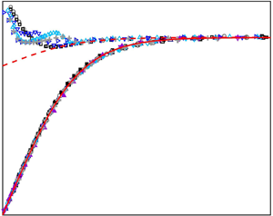
In figure 5, we show $(T_h - T)/(T_h - T_o)$ as a function of $z/\lambda _h$, measured at $x/L = 0.95$ and $0.99$ above the heating plate. We choose the data for $Ra \lesssim 6 \times 10^{10}$ in order to exclude the $Nu$ oscillation effects on the BL structures, and we take the averaged $\chi = 0.82$ over the $Ra$ range. It is found that the three dimensionless profiles for $x/L = 0.95$ scale with $\lambda _h$ for $z/\lambda _h \lesssim 2.2$, and they are well described by (4.5) with $\xi _p = 1.6$ and $b = 0.77$. In the cold region, the three profiles almost overlap as well, since the ratio of $\lambda _c / \lambda _h$ is nearly constant $\approx 0.28$ for these values of $Ra$.

Figure 5. Measured $(T_h - T)/(T_h - T_o)$ as a function of $z/\lambda _h$, measured at $x/L = 0.95$ and $0.99$ for varying $Ra$. For these measurements, $\chi = 0.82$. The black dashed line represents (4.1) with $\xi _p = 0.44$ and $a=0.69$. The red solid line is (4.5) with $\xi _p = 1.6$ and $b = 0.77$.

The black dashed line in figure 5 represents the same calculated $T$-values as those in figure 4(b), but re-scaled in a different dimensionless form. The ratio of $\xi _p = 1.6$ for the hot region to $\xi _p = 0.44$ for the cold region is consistent with the ratio of $\lambda _c / \lambda _h$. Note that for $x/L = 0.95$ the two fitting ranges intersect at the same temperature. It indicates that the hot and cold regions are nearly adjacent to each other, which forms a double-BL structure above the heating plate. At $x/L = 0.99$ near the vertical sidewall, the normalized $T$-data are almost constant around $z/\lambda _h= 2.2$, close to the interface between the two regions. It may be caused by the mixing of uprising thermal plumes. As $Ra$ increases, both the mixing intensity and the separation of the two scales increase. Above a certain $Ra$, (for instance, when $Ra \simeq 10^{12}$, $\lambda _c / \lambda _h = 10$), the double-BL structure is expected to be highly unstable and HC eventually transits to a chaotic state.

5. Summary

We presented experimental results for the time-averaged vertical temperature profiles $\theta$ near the thermal BLs at the bottom of HC samples over the range $2 \times 10^{10} \lesssim Ra \lesssim 9 \times 10^{12}$ and for $Pr \simeq 6$ and demonstrated that the profiles scale with the thicknesses $\lambda _c$ and $\lambda _h$ of, respectively, cold and hot thermal BLs. Near the cold thermal BL, all temperature profiles have a universal scaling form $\theta (z/\lambda _c)$ for $0 \lesssim z/\lambda _c \lesssim 3.5$. Under assumption of a single maximum in the vertical profile of the large-scale horizontal velocity $U$ near the BL, we derived (3.10) for $\theta (z/\lambda _c)$ that can well describe the collapsing experimental $\theta (z/\lambda _c)$ profiles.

The $\theta$-profile above the heating plate has, however, a more complicated structure, which can be split into two regions. In the hot region below, the $\theta$ data scale with the similarity variable $z/\lambda _h$, while in the cold region above, they scale with $z/\lambda _c$. In both regions, the shapes of the profiles are in good agreement with the predicted form (3.10) for laminar BL. The result thus reveals a double-layer structure for the temperature field above the heated plate. For $Ra \lesssim 6\times 10^{10}$, the scaling ranges of the two regions nearly coincide, which indicates that the entire hot thermal BL is laminar. As $Ra$ increases, the increasing scale separation allows fluctuations in the hot region. In the range $10^{11} \lesssim Ra \lesssim 4.3 \times 10^{11}$, local $\theta$-profiles have spatial oscillations for $\lambda _h \lesssim z \lesssim \lambda _c$. Above $Ra \simeq 10^{12}$, at which $\lambda _c/\lambda _h \simeq 10$, there are more fluctuations in the hot region that render the shape of $\theta$ further different from what can be predicted with the laminar BL equation. The profiles in the cold region, however, still follow the laminar equation. This suggests that the rest of the HC flow remains to be rather laminar. The change of the scaling form $\theta (z/\lambda _h)$ in the hot region with growing $Ra$ is consistent with the change of the $Nu$ dependence on $Ra$ observed by Reiter & Shishkina (Reference Reiter and Shishkina2020).