3.1. Global quantities

As we study low-$Pr$ convection in a 2-D domain, we first compare the scaling of the global quantities in our simulations with those observed in 3-D RBC for $Pr \approx 0.021$.

The Reynolds number $Re$, which is a measure of the turbulent momentum transport in the flow, is another important global quantity in RBC. We compute $Re$ in our flow as

(3.1)\begin{equation} Re = \sqrt{Ra/Pr} \,u_{rms}, \end{equation}

with the rms velocity $u_{rms}$ defined as

(3.2)\begin{equation} u_{rms} = \sqrt{\langle u_x^2+u_z^2 \rangle_{A,t}}. \end{equation}

Important theoretical models in RBC that yield the scaling relations for global quantities such as $Nu$ and $Re$ (Shraiman & Siggia Reference Shraiman and Siggia1990; Grossmann & Lohse Reference Grossmann and Lohse2000) assume the existence of a large-scale structure of the order of the size of the cell. For instance, the Shraiman & Siggia (Reference Shraiman and Siggia1990) theory provides the scalings of $Nu$ and $Re$ by considering the properties of (2-D) viscous and thermal BLs generated due to the shear applied by the LSC. Similarly, the Grossmann–Lohse model (Grossmann & Lohse Reference Grossmann and Lohse2000) is based on the existence of an LSC in the convection cell, which is characterized by a single velocity scale. Thus, the above scaling theories are applicable in both 2-D and 3-D RBC (van der Poel et al. Reference van der Poel, Stevens and Lohse2013; Zhu et al. Reference Zhu, Mathai, Stevens, Verzicco and Lohse2018). As the LSC also exists in our low-$Pr$ 2-D RBC for all the Rayleigh numbers, it is interesting to compare the global quantities in our flow with those observed in 3-D RBC for similar governing parameters, where the LSC structure is also observed.

We compute the Nusselt and Reynolds numbers using (2.5) and (3.1) for all our simulation runs and plot them as a function of $Ra$ in figure 1. To compare our $Nu$ and $Re$ with those obtained in a 3-D RBC, we also show $Nu$ and $Re$ for $Pr = 0.021$ from Scheel & Schumacher (Reference Scheel and Schumacher2017), who investigated low-$Pr$ RBC in a cylindrical cell of aspect ratio one from $Ra = 3 \times 10^5$ to $Ra = 4 \times 10^8$. Thus their governing parameters are very similar to the parameters in the present study, and due to the existence of a similar large-scale structure in both these flows, it is interesting to compare the global heat and momentum transports between these flows. Figure 1(a) reveals that $Nu$ in our 2-D RBC increases as $Ra^\gamma$ and agrees reasonably well with that of Scheel & Schumacher (Reference Scheel and Schumacher2017). The best fit to our data yields $Nu = (0.20 \pm 0.004)Ra^{0.25\, \pm \, 0.003}$, which is close to $Nu = (0.13 \pm 0.04)Ra^{0.27\, \pm \, 0.01}$ as observed by Scheel & Schumacher (Reference Scheel and Schumacher2017) for nearly the same range of $Ra$. The exponent $\gamma = 0.25$ in our flow is smaller than the exponent $\gamma \approx 0.30$ observed for $Pr = 0.7$ and $Pr = 5.3$ in 2-D RBC with a similar flow configuration (Zhang et al. Reference Zhang, Zhou and Sun2017b). The lower $\gamma$ in our low-$Pr$ 2-D RBC is similar to that observed in 3-D RBC, where $\gamma$ also decreases with decreasing $Pr$ (Scheel & Schumacher Reference Scheel and Schumacher2017). Note that the Grossmann–Lohse theory (Grossmann & Lohse Reference Grossmann and Lohse2000) also predicts a lower $\gamma$ for convection in low-$Pr$ fluids than for convection in moderate- and high-$Pr$ fluids.

Figure 1. The Nusselt and Reynolds numbers as a function of $Ra$ in our 2-D RBC (circles) and those obtained by Scheel & Schumacher (Reference Scheel and Schumacher2017) for $Pr = 0.021$ in a cylindrical cell of aspect ratio unity (squares). A reasonably good agreement of $Nu$ in both 2-D and 3-D RBC for $Pr = 0.021$ is observed.

We would like to point out that even the magnitudes of $Nu$ obtained in our 2-D flows are very similar to those obtained by Scheel & Schumacher (Reference Scheel and Schumacher2017). This is remarkable and indicates that, at least in the present range of parameters, the LSC is probably the most dominant mode of heat transport in both the 2-D and the 3-D RBC. Van der Poel et al. (Reference van der Poel, Stevens and Lohse2013) also compared $Nu$ between 2-D and 3-D RBC with similar flow configurations and noticed that the values of $Nu$ at $Ra = 10^8$ are closer in 2-D and 3-D RBC for low Prandtl numbers, whereas a stronger deviation was observed at moderate Prandtl numbers. In an earlier study, however, Schmalzl, Breuer & Hansen (Reference Schmalzl, Breuer and Hansen2004) observed that the integral quantities in 2-D and 3-D RBC differ for low Prandtl numbers, whereas they are similar for high Prandtl numbers (van der Poel et al. Reference van der Poel, Stevens and Lohse2013; Pandey et al. Reference Pandey, Verma, Chatterjee and Dutta2016). However, the sizes of the flow domains in the 2-D and 3-D cases were different, and a smaller $Ra = 10^6$ was used in Schmalzl et al. (Reference Schmalzl, Breuer and Hansen2004). Interestingly, the scaling $Nu \sim Ra^{0.25}$ in our 2-D RBC agrees well with the existing literature for $Pr \approx 0.021$ in 3-D RBC, as $\gamma \approx 0.25$ has been observed in various earlier investigations (Cioni et al. Reference Cioni, Ciliberto and Sommeria1997; Glazier et al. Reference Glazier, Segawa, Naert and Sano1999; Grossmann & Lohse Reference Grossmann and Lohse2000; Pandey & Verma Reference Pandey and Verma2016; Zürner et al. Reference Zürner, Schindler, Vogt, Eckert and Schumacher2019). Note, however, that the structure and the characteristics of LSC are more complex in 3-D RBC, where it has a quasi-2-D character and exhibits twisting and sloshing modes in addition to azimuthal reorientations in a cylindrical cell (Wagner et al. Reference Wagner, Shishkina and Wagner2012; Schumacher et al. Reference Schumacher, Bandaru, Pandey and Scheel2016; Zwirner et al. Reference Zwirner, Khalilov, Kolesnichenko, Mamykin, Mandrykin, Pavlinov, Shestakov, Teimurazov, Frick and Shishkina2020), which are clearly absent in 2-D RBC. Therefore, the observed similarity between the $Nu$–$Ra$ scaling in our low-$Pr$ convection and that in 3-D RBC requires a more detailed investigation, which is beyond the scope of the present work.

Figure 1(b) exhibits the Reynolds number in our simulations as a function of $Ra$, along with the $Re$ for $Pr = 0.021$ from Scheel & Schumacher (Reference Scheel and Schumacher2017). It is clear that the Reynolds numbers in our 2-D RBC are consistently higher than those in the 3-D RBC, for all $Ra$. The best fit in the range of $Ra$ from $10^6$ to $10^9$ yields $Re = (1.47 \pm 0.24)Ra^{0.60\, \pm \, 0.02}$, which is different from the result $Re \sim Ra^{0.45}$ observed in 3-D RBC for $Pr \approx 0.021$ (Pandey & Verma Reference Pandey and Verma2016; Scheel & Schumacher Reference Scheel and Schumacher2017). Note that the magnitude of the Reynolds numbers and the exponent in the $Re$–$Ra$ scaling in 2-D RBC have also been observed to be higher than those in 3-D RBC for moderate and high Prandtl numbers (van der Poel et al. Reference van der Poel, Stevens and Lohse2013; Zhang et al. Reference Zhang, Zhou and Sun2017b). Thus, the exponent in the $Re$–$Ra$ scaling in 2-D RBC appears to remain nearly the same ($\approx 0.6$) for a wide range of Prandtl numbers (van der Poel et al. Reference van der Poel, Stevens and Lohse2013; Pandey et al. Reference Pandey, Verma, Chatterjee and Dutta2016; Zhang et al. Reference Zhang, Zhou and Sun2017b). The larger magnitude of $Re$ in our flow is probably due to the more coherent motion of the thermal plumes in 2-D RBC than in 3-D RBC (Zhang et al. Reference Zhang, Huang, Jiang, Liu, Lu, Qiu and Zhou2017a).

To summarize, the scaling of $Nu$ in our 2-D RBC, which is related to the scaling of the mean thermal BL thickness, is very similar to that observed in 3-D RBC for $Pr \approx 0.021$. Therefore, the characteristics of the thermal BL in our 2-D convection may also be similar to those in 3-D RBC for low Prandtl numbers.

3.2. Flow structure

The thermal plumes emitted from the top and bottom plates in an RBC cell of aspect ratio around unity move coherently by forming an LSC, which we also detect in our simulations. For all the Rayleigh numbers, we observe that the LSC rotates in a single direction for the entire duration of the simulation and thus does not exhibit any flow reversal (Sugiyama et al. Reference Sugiyama, Ni, Stevens, Chan, Zhou, Xi, Sun, Grossmann, Xia and Lohse2010; Chandra & Verma Reference Chandra and Verma2013; Podvin & Sergent Reference Podvin and Sergent2015; Pandey et al. Reference Pandey, Verma and Barma2018b; Zhang et al. Reference Zhang, Xia, Zhou and Chen2020). Specifically, in our simulations the LSC rotates in the clockwise direction for $Ra = 10^6$, $Ra = 10^8$ and $Ra = 10^9$, and in the counterclockwise direction for $Ra = 5 \times 10^5$ and $Ra = 10^7$. Therefore, for the consistency of our further analyses and discussions, we transform the horizontal velocity and temperature fields for $Ra = 5 \times 10^5$ and $Ra = 10^7$ by reflecting them about the plane $x = L/2$, which changes the direction of LSC. As a result, the LSC rotates in the clockwise direction in all our simulations.

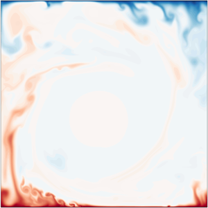
We exhibit the instantaneous temperature field for $Ra = 10^6$ to $Ra = 10^9$ in figure 2, along with the instantaneous velocity vectors. We observe that because the Kolmogorov and Batchelor length scales decrease with increasing $Re$ or $Ra$, the finest thermal structures in the flow, which are coarser for $Ra = 10^6$, become finer with increasing $Ra$. Also, the thickness of the thermal plumes, which are emitted mostly from the bottom left and top right parts of the plates, decreases with increasing $Ra$. This is because the width of the thermal plumes is similar to the thickness of the thermal BLs (Zhou, Sun & Xia Reference Zhou, Sun and Xia2007; Shishkina & Wagner Reference Shishkina and Wagner2008), which decreases with increasing $Ra$. We also show the time-averaged flow structure for $Ra = 10^6$ to $Ra = 10^9$ in figure 3, which reveals that the mean LSC structure is octagonal (or circular) in our low-$Pr$ RBC. The corner flow structures become weaker and the LSC becomes increasingly squarish with increasing $Ra$ in our flow. The mean flow structure in our low-$Pr$ RBC is different from the mean flow structures in moderate- and high-$Pr$ 2-D RBC for similar Rayleigh numbers, where the LSC is usually observed to be aligned along a diagonal of the cell (Sugiyama et al. Reference Sugiyama, Ni, Stevens, Chan, Zhou, Xi, Sun, Grossmann, Xia and Lohse2010; Zhou et al. Reference Zhou, Sugiyama, Stevens, Grossmann, Lohse and Xia2011; Chandra & Verma Reference Chandra and Verma2013; Zhang et al. Reference Zhang, Huang, Jiang, Liu, Lu, Qiu and Zhou2017a,b).

Figure 2. Instantaneous temperature (colours) and velocity (vector) fields in the entire simulation domain for (a) $Ra = 10^6$, (b) $Ra = 10^7$, (c) $Ra = 10^8$ and (d) $Ra = 10^9$. Increasingly finer thermal structures are observed in the flow with increasing $Ra$. Also, the primary flow structure, i.e. the LSC, becomes stronger, whereas the secondary structures become weaker with increasing $Ra$.

Figure 3. Time-averaged flow structure for (a) $Ra = 10^6$, (b) $Ra = 10^7$, (c) $Ra = 10^8$ and (d) $Ra = 10^9$. The temperature (colours) and the velocity (vector) fields, averaged for the entire duration of simulations, exhibit that the LSC structure gets increasingly developed, i.e. occupies a larger fraction of the flow domain, with increasing $Ra$.

Figure 2 also shows that, in addition to a large-scale structure, smaller structures are also present in the flow. The strengths of the flow structures of various sizes, also known as the flow modes, vary during the evolution of the flow due to the nonlinear interactions (Chandra & Verma Reference Chandra and Verma2013). See also the supplementary movies available at https://doi.org/10.1017/jfm.2020.961, which show the temporal evolution of our low-$Pr$ flow for each $Ra$. We estimate the strengths of various flow modes by computing their kinetic energy content by projecting the velocity field on a sine–cosine basis (Wagner & Shishkina Reference Wagner and Shishkina2013; Chen et al. Reference Chen, Huang, Xia and Xi2019) as follows:

(3.3)\begin{gather} u_x({\boldsymbol x},t) = \sum_{m,n} \hat{u}_x(m,n,t) [-2 \sin (m {\rm \pi}x) \cos (n {\rm \pi}z)], \end{gather}

(3.4)\begin{gather}u_z({\boldsymbol x},t) = \sum_{m,n} \hat{u}_z(m,n,t) [2 \cos (m {\rm \pi}x) \sin (n {\rm \pi}z)]. \end{gather}

Here $m,n \in I$, i.e. they are positive integers. A flow mode with indices $(m,n)$ represents the flow structure with $m$ horizontally-stacked rolls and $n$ vertically-stacked rolls. Thus, the LSC is represented by the $(1,1)$-mode, and the smaller flow structures, such as the corner rolls, are represented by modes with higher indices (Chandra & Verma Reference Chandra and Verma2013; Wagner & Shishkina Reference Wagner and Shishkina2013; Pandey et al. Reference Pandey, Verma and Barma2018b; Chen et al. Reference Chen, Huang, Xia and Xi2019). We exhibit the flow structures corresponding to a few dominant modes in our flow in figure 4(a–d).

Figure 4. Flow structures corresponding to the (a) $(1,1)$-mode, (b) $(3,1)$-mode, (c) $(1,3)$-mode and (d) $(2,2)$-mode. (e) Fraction of the total kinetic energy contained in these flow modes as a function of $Ra$. In the turbulent regime, i.e. for $Ra \geq 10^7$, the strength of the LSC, which is represented by the $(1,1)$-mode, increases with increasing $Ra$. Moreover, strong corner flow structures, approximately represented by the (2,2)-mode, are present in the flow for $Ra = 10^6$.

The amplitude of the modes is computed as $\hat {u}_x(m,n) = \langle -2 u_x({\boldsymbol x}) \sin (m {\rm \pi}x) \cos (n {\rm \pi}z) \rangle _A$ and $\hat {u}_z(m,n) = \langle 2 u_z({\boldsymbol x}) \cos (m {\rm \pi}x) \sin (n {\rm \pi}z) \rangle _A$, and the kinetic energy contained in a mode $(m,n)$ is given by

(3.5)\begin{equation} E(m,n) = |\hat{u}_x(m,n)|^2 + |\hat{u}_z(m,n)|^2. \end{equation}

We compute the time-averaged kinetic energy of various flow modes by considering $m, n = 1\text {--}10$, and plot the fraction of the total kinetic energy $E = \langle u_x^2 + u_z^2 \rangle _{A,t}$ contained in a few strongest modes in our flow as a function of $Ra$ in figure 4(e). Figure 4(e) reveals that for $Ra = 5 \times 10^5$, the flow is primarily dominated by one large-scale structure, which becomes weaker for $Ra = 10^6$ due to the growth of the smaller flow structures. This can be confirmed from the supplementary movies and from figure 2(a), which show that strong corner flow structures (represented approximately by the (2,2)-mode) are present in the flow at $Ra = 10^6$. The strength of the LSC further decreases for $Ra = 10^7$ as even smaller structures are generated due to the increased Reynolds number of the flow. However, for $Ra \geq 10^7$, the strength of the LSC (i.e. of the (1,1)-mode) grows and the total strength of the small-scale structures decays with increasing $Ra$ (Sugiyama et al. Reference Sugiyama, Ni, Stevens, Chan, Zhou, Xi, Sun, Grossmann, Xia and Lohse2010; Chandra & Verma Reference Chandra and Verma2013). This indicates that with increasing $Ra$ the LSC structure gets more and more squarish and increasingly fills the entire domain in our low-$Pr$ RBC (Lui & Xia Reference Lui and Xia1998; Niemela & Sreenivasan Reference Niemela and Sreenivasan2003).

Furthermore, we observe that the evolution of the flow for $Ra = 5 \times 10^5$ is unsteady and periodic time-dependent, while for $Ra = 10^6$ it is nearly periodic, i.e. some non-periodicity sets in the flow. To depict this, we look at the time trace of the temperature field at a fixed probe in the flow. Figure 5 shows a segment of the temperature trace at a probe located at the centre of the bottom plate near the thermal BL height, i.e. at $x_0 = L/2$, $z_0 \approx \delta _{\langle T \rangle }$. Figure 5(a) reveals that the temperature signal is periodic for $Ra = 5 \times 10^5$, whereas figure 5(b) shows that some non-periodicity appears in the signal for $Ra = 10^6$. The temperature field at the probe for $Ra \geq 10^7$ varies chaotically, indicating that the flow for $Ra \geq 10^7$ is turbulent (see also supplementary movies).

Figure 5. A segment of the time traces of the temperature field at a fixed probe near the centre of the bottom plate at the thermal BL height, i.e. at $x_0 = L/2$, $z_0 \approx \delta _{\langle T \rangle }$, for (a) $Ra = 5 \times 10^5$, (b) $Ra = 10^6$, (c) $Ra = 10^7$, (d) $Ra = 10^8$ and (e) $Ra = 10^9$ (taken from run 5a). Panel (a) shows that the flow is periodic for $Ra = 5 \times 10^5$, whereas the flow is nearly periodic for $Ra = 10^6$, as indicated by the signal in panel (b). The temperature at the probe varies chaotically in (c–e), indicating that the flow is turbulent for $Ra \geq 10^7$.

Unlike the flow in a pipe or channel, the RBC flow in a confined domain is not homogeneous in the horizontal directions. Instead, the horizontal plates can be divided into three distinct flow regions. For RBC in a domain of aspect ratio around unity, the hot plumes are generated primarily near one of the sidewalls and ascend towards the cold plate along that sidewall. Similarly, the cold plumes detaching from the top plate descend towards the hot plate along the opposite sidewall. These two regions are called respectively the plume-ejection and plume-impact regions (van der Poel et al. Reference van der Poel, Ostilla-Mónico, Verzicco, Grossmann and Lohse2015; Schumacher et al. Reference Schumacher, Bandaru, Pandey and Scheel2016; Zhu et al. Reference Zhu, Mathai, Stevens, Verzicco and Lohse2018). In between these two regions, there exists a shear-dominated region, where the LSC is nearly parallel to the horizontal plates. We also depict these regions in our flow in a caricature in figure 6. Due to this specific flow morphology of RBC in a confined domain, the thermal and viscous BL profiles have often been studied in the shear-dominated central region (Zhou et al. Reference Zhou, Stevens, Sugiyama, Grossmann, Lohse and Xia2010; van der Poel et al. Reference van der Poel, Stevens and Lohse2013; Schumacher et al. Reference Schumacher, Bandaru, Pandey and Scheel2016; Wang et al. Reference Wang, Xu, He, Yik, Wang, Schumacher and Tong2018). In this study, however, we compute the local temperature profiles in the aforementioned three regions and find that the BL profiles in the shear and impact regions are similar, and differ from the profiles in the ejection region.

Figure 6. A caricature exhibiting the plume-ejection, shear-dominated and plume-impact regions at the top and bottom plates in our low-$Pr$ 2-D RBC. An instantaneous snapshot of the temperature field for $Ra = 10^9$ is used to depict these regions.

4.1. Local boundary layer thicknesses

We observe for all $Ra$ that the central region near the plates is dominated by shear generated due to LSC, and therefore, the flow properties at $x \approx L/2$ are similar to those in a shear flow. The locations $x = L/4$ and $x = 3L/4$ at the bottom plate in our flow approximately correspond to the plume-ejection and plume-impact regions; i.e. the hot plumes are ejected from the bottom plate mostly at $x \approx L/4$ and the cold plumes impact at the bottom plate mostly at $x \approx 3L/4$ (see figure 2). The situation is reversed at the top plate; i.e. the physical location of the ejection region at the bottom corresponds to the impact region at the top, and vice versa. (See also figure 6, where we have summarized these flow regions at the plates in a caricature.) We have analysed the properties of the temperature profiles measured at several locations in the flow. However, for clarity, we will mainly discuss the profiles measured at $x=L/4$, $x=L/2$ and $x=3L/4$, as these positions at the bottom plate typically correspond to the ejection, shear and impact regions, respectively. We would like to point out that the large-scale structures in our flow fluctuate strongly in time (see supplementary movies), which causes the flow properties at the aforementioned locations to be occasionally influenced by the properties from the other regions. Therefore, we inevitably sample a mixed statistics due to the use of an immovable observational window in the flow.

We show the time-averaged temperature profiles at $x=L/4$, $x=L/2$ and $x=3L/4$ for $Ra = 10^6$ to $Ra = 10^9$ in figure 7. To reduce the scatter, we average the profiles in a tiny neighbourhood around the aforementioned locations. Specifically, the profile at $x_0$ is averaged in the region corresponding to $x_0-0.02L \leq x \leq x_0+0.02L$, where $x_0 = L/4, L/2, 3L/4$. Figure 7 shows that the profiles at $x = L/2$ are nearly symmetric about the midplane, as $x \approx L/2$ corresponds to the shear-dominated region at both the top and bottom plates. The profiles at $x \neq L/2$, however, are not symmetric about the midplane. For instance, we can see in figure 7(d) for $Ra = 10^9$ that the profile near the bottom (top) plate at $x=L/4$ ($x=3L/4$), which corresponds to the ejection region, approaches the bulk temperature slowly compared to the profiles in the other two regions. This is because the hot (cold) plumes that are ejected from the bottom (top) plate in the ejection region carry their thermal energy for a longer time and travel farther in the bulk region before losing their heat due to thermal diffusion. Moreover, the profile near the bottom (top) plate at $x = 3L/4$ ($x=L/4$), which corresponds to the impact region, looks similar to that at $x=L/2$ in the shear region. Figure 7 shows that the local profiles for all the Rayleigh numbers exhibit similar behaviour. Thus, to conclude, the temperature profiles in the impact and shear regions are similar, whereas the temperature profile in the ejection region differs from them. Therefore, from now on, we will discuss the properties of the temperature profiles based on whether they belong to the impact, ejection or shear region, and not based on their physical location in the flow domain.

Figure 7. Time-averaged temperature profiles measured at different horizontal positions for (a) $Ra = 10^6$, (b) $Ra = 10^7$, (c) $Ra = 10^8$ and (d) $Ra = 10^9$. For all $Ra$, profiles at $x=L/2$ are symmetric about the midplane, whereas those at $x \ne L/2$ do not exhibit symmetry, because of the differing flow properties at the opposite plates at the particular physical location. In all the panels, blue curves near the bottom plate are similar to green curves near the top plate, and vice versa.

We compute the local thermal BL width $\delta _T(x)$ using the slope method (Zhou et al. Reference Zhou, Sugiyama, Stevens, Grossmann, Lohse and Xia2011; Scheel et al. Reference Scheel, Kim and White2012; Wagner et al. Reference Wagner, Shishkina and Wagner2012), where $\delta _T(x)$ is estimated as the distance from the plate where the slope of the temperature profile drawn at the plate meets the horizontal line passing through the first minimum of the profile. In figure 8, we demonstrate this method of determining the BL thickness from the instantaneous temperature profiles measured at two different positions at the plate. Figure 8 shows that the profiles do not always approach the bulk temperature monotonically, and the first minimum may differ from the bulk temperature. We also compute the instantaneous BL thicknesses using the local vertical temperature gradient at the plate as $\delta _T(x) = 0.5/|\partial T(x)/\partial z|_{z=0}$, which is equivalent to computing the BL thickness using the slope method with the horizontal line drawn at the mean temperature ${\rm \Delta} T/2$. We find that the mean (and most of the time instantaneous) BL thicknesses determined using this method are nearly the same as those obtained using the first minimum method. However, we prefer the first minimum method to include the instantaneous variation of the profiles, as the temperature in the bulk region may instantaneously differ from ${\rm \Delta} T/2$.

Figure 8. Instantaneous local temperature profiles (a,b) and their magnifications near the bottom plate (c,d) to demonstrate the determination of the instantaneous local thermal BL thickness using the slope method. Panels (a) and (c) show a profile measured in the shear-dominated region at $x_0 = L/2$ for $Ra = 10^8$; panels (b) and (d) show a profile measured in the plume-ejection region at $x_0 = L/4$ for $Ra = 10^9$. Position of the intersection of the horizontal line drawn at the first minimum with the slope at the plate yields $\delta _T(x_0,t)$. Panels (a) and (b) show that the temperature at the first minimum may differ from $T_{bulk} = {\rm \Delta} T/2$. Inset in (c,d) indicates the linear variation of temperature in the vicinity of the bottom plate.

To explore the structure of the thermal BL, we compute the local BL thicknesses $\delta _{\langle T \rangle }(x)$ at both the plates using the time-averaged temperature profiles. Figure 9 shows the local BL width averaged over the top and bottom plates and normalized with the BL width at $x=L/2$. Note that due to the interchange of the ejection and impact regions, local BL thickness at a position $x$ in figure 9 is the average of $\delta _{\langle T \rangle }(x)$ at the bottom and $\delta _{\langle T \rangle }(L-x)$ at the top plate. Figure 9 reveals that the BL structure is similar for all the explored $Ra$ in our low-$Pr$ RBC. We observe that $\delta _{\langle T \rangle }(x)$ is the largest near the sidewalls and decreases as one moves towards the central region. Moreover, the local thicknesses are larger in the ejection region than in the other two regions, as indicated in figure 9(a). We also find that the values of $\delta _{\langle T \rangle }(x)$ in the impact region are a bit smaller than those in the shear region. To show the BL structure away from the sidewalls, we plot $\delta _{\langle T \rangle }(x)$ for $0.2L \leq x \leq 0.8L$ in figure 9(b), which reveals that the BL structure is nearly independent of $Ra$ in the impact and shear regions. In the ejection region, however, the variation of the normalized BL thickness depends on $Ra$. We quantify the relative variation of the BL thicknesses exhibited in figure 9(b) as

(4.1)\begin{equation} \mathcal{R} = \frac{[\delta_{\langle T \rangle}(x)]_{max}- [\delta_{\langle T \rangle}(x)]_{min}}{[\delta_{\langle T \rangle}(x)]_{min}}, \end{equation}

where $[\delta _{\langle T \rangle }(x)]_{max}$ and $[\delta _{\langle T \rangle }(x)]_{min}$ are respectively the maximum and minimum BL thicknesses over the central region, i.e. in the region $0.2L \leq x \leq 0.8L$ at the plate. We find $\mathcal {R} = 3.1, 1.9, 1.5, 1.0, 1.6$ respectively for $Ra = 5 \times 10^5, 10^6, 10^7, 10^8,10^9$, which indicates that $\mathcal {R}$ generally decreases with increasing $Ra$ in our flow. Our data at $Ra = 10^9$ do not follow the decreasing trend very well, which might be due to a limited statistics available for this $Ra$. A few more simulations at intermediate Rayleigh numbers would probably yield a better picture of the BL structure in the ejection region in our low-$Pr$ flow.

Figure 9. (a) Variation of the normalized local BL thicknesses along the horizontal plate computed using the time-averaged profiles. Except very close to the sidewalls, the local thicknesses $\delta _{\langle T \rangle }(x)$ are larger in the ejection region and decrease as the impact region is approached; i.e. the thickness grows in the direction of LSC. (b) Magnification of (a) exhibiting the BL structure in the central region away from the sidewalls, which shows that the BL structure is nearly independent of $Ra$ in the impact and shear regions.

According to the Prandtl–Blasius BL theory, the BL thickness grows as $\sqrt {x}$ in the downstream direction for a laminar BL, whereas it grows linearly with $x$ for a turbulent BL (Schlichting & Gersten Reference Schlichting and Gersten2004). In our 2-D RBC, the hotter or colder fluid impinges on the plate in the impact region and then moves along the plate towards the ejection region. We thus also observe a growth of the BL thickness in the downstream direction, i.e. in the direction of the LSC on the plate. However, $\delta _{\langle T \rangle }(x)$ in our low-$Pr$ RBC does not follow either of the aforementioned scalings. Possible reasons for a different BL structure in our flow might be the assumptions in the Prandtl–Blasius BL theory, which are not totally satisfied in our 2-D convection flow. For example, the BLs in our flow are not entirely laminar and the turbulent fluctuations within the BL region become stronger with increasing $Ra$ (see figure 16b). We moreover observe that the BL structure is not symmetric about the centre of the plate, which is qualitatively similar to observations made for high-$Pr$ 2-D RBC (Werne Reference Werne1993; Zhou et al. Reference Zhou, Sugiyama, Stevens, Grossmann, Lohse and Xia2011). Our observations of the BL structure in our low-$Pr$ convection are also qualitatively similar to those of Wagner et al. (Reference Wagner, Shishkina and Wagner2012) in a cylindrical cell of aspect ratio one, where the BL width increases in the direction of LSC, as well as to the observations of Scheel & Schumacher (Reference Scheel and Schumacher2014) that the local BL widths are larger in the plume-ejection region. Wagner et al. (Reference Wagner, Shishkina and Wagner2012), however, observed a nearly linear growth of the BL thickness along the direction of LSC. Our results are also different from those of Lui & Xia (Reference Lui and Xia1998), who studied the thermal BL structure in a cylindrical cell of aspect ratio one filled with water and observed that, in the plane of LSC, the BL width is minimum at the centre of the plate and increases symmetrically towards the sidewalls. The aforementioned differences between the BL structure in our 2-D RBC and those observed in 3-D RBC, therefore, indicate that the quasi-2-D nature and other characteristics of LSC in 3-D RBC also affect the BL structure.

We compute the local thermal BL thicknesses $\delta _{\langle T \rangle }(x_0)$ at $x_0 = L/4$, $x_0 = L/2$ and $x_0 = 3L/4$ using the time-averaged profiles exhibited in figure 7 and find that $\delta _{\langle T \rangle }(x_0)$ decreases with increasing $Ra$ as $Ra^{-\beta (x_0)}$, with the exponent $\beta (x_0)$ depending on the position at the plate. In figure 10(a), we plot $\delta _{\langle T \rangle }(x_0)$ averaged over the corresponding regions at the top and bottom plates as a function of $Ra$, which reveals that the BL thicknesses in the impact and shear regions are similar for all $Ra$. This is consistent with the fact that the profiles in the shear and impact regions exhibited in figure 7 are also similar. The best fit yields that $\delta _{\langle T \rangle }(x_0)/H$ varies as $(1.4 \pm 0.2)Ra^{-0.23 \,\pm \, 0.01}$ in the shear region and as $(1.5 \pm 0.1)Ra^{-0.24 \,\pm \, 0.01}$ in the impact region. The local BL thicknesses in the ejection region, however, are larger than those in the other two regions for all $Ra$, and scale as $(8.9 \pm 1.1)Ra^{-0.30\, \pm \, 0.02}$.

Figure 10. (a) Local thermal BL thicknesses averaged over both the plates vary as $Ra^{-\beta (x)}$ in the ejection, shear and impact regions, with $\beta (x_0)$ being larger in the ejection region. The black dashed line indicates the scaling of the BL thickness $\delta _{\langle T \rangle }$ computed using the horizontally- and temporally-averaged profiles (shown in figure 12b). If these scalings hold for the larger Rayleigh numbers, the blue line will intersect the red or green line at $Ra^* \approx 8 \times 10^{12}$, beyond which the thermal BL might become uniform at the plate. (b) Variation of the local scaling exponent $\beta (x)$ along the plate obtained from the BL thicknesses averaged over the top and bottom plates. The dashed horizontal line indicates the scaling exponent of the mean BL thickness. The direction of LSC and the ejection, shear and impact regions are also indicated.

We further explore the variation of the local exponent $\beta (x)$ at the plate by computing it from the local BL thicknesses. Figure 10(b) exhibits the local exponents $\beta (x)$ computed from the averaged BL thicknesses at both the plates in the central region far from the sidewalls. We observe that the $\beta (x)$ values are larger in the ejection region than in the shear and impact regions, where they are nearly the same. Note that the thermal BL thickness is related to the diffusive heat flux at the plate. To understand the position-dependent variation of the properties of the thermal BL, we compute the diffusive fraction of the total heat flux as $F_{diff}(x_0) = (H \partial \langle T \rangle _t(x_0)/\partial z)/(Nu {\rm \Delta} T)$ in the ejection, shear and impact regions. Figure 11(a) shows $F_{diff}(x_0)$ as a function of $z/\delta _{\langle T \rangle }$ in the ejection region, while figure 11(b) shows $F_{diff}(x_0)$ in the shear region (solid curves) and the impact region (dash-dot curves). We observe for all $Ra$ that the values of $F_{diff}(x_0)$ at the plate and in its vicinity in the ejection region are smaller than those in the shear region, which in turn, are a bit smaller than those in the impact region. This is because of a larger temperature gradient in the impact region due to impinging cold (hot) plumes at the bottom (top) plate. As the BL width is inversely proportional to the vertical temperature gradient (or the diffusive flux) at the plate, this implies that the local BL thickness in the ejection region is larger than the thicknesses in the shear and impact regions, which is consistent with the BL structure from figure 9.

Figure 11. Vertical profiles of the fraction $F_{diff}(x_0)$ of the total heat flux carried by the thermal diffusion in (a) the ejection region and (b) the shear region (solid curves) and impact region (dash-dot curves) within the BL. The values of $F_{diff}(x_0)$ at the plate are smaller in the ejection region than in the shear and impact regions, and with increasing $Ra$, $F_{diff}(x_0)$ is generally increasing in the ejection region and decreasing in the other two regions.

Furthermore, we observe that $F_{diff}(x_0)$ in the vicinity of the plate is generally increasing in the ejection region, but decreasing in the shear and impact regions, with increasing $Ra$. This means that with increasing $Ra$, the BL width in the ejection region decreases faster, whereas the BL widths in the other two regions decrease slower, compared to the mean BL thickness, which agrees with the observations of figure 10. Therefore, for moderately large Rayleigh numbers in our low-$Pr$ flow, the difference between the diffusive contributions from various regions is decreasing, or, in other words, the variation of the diffusive heat flux over the plate becomes weaker with increasing $Ra$. The reason for this weaker variation is the increasing strength of LSC with increasing $Ra$ in our flow (Lui & Xia Reference Lui and Xia1998), as we have observed that the (1,1)-mode representing the LSC structure becomes stronger as $Ra$ increases (see figure 4e). A stronger LSC causes the cold (hot) plumes impinging on the bottom (top) plate in the impact region to move a larger distance along the plate before their heat is lost due to thermal diffusion. This causes an increasingly uniform temperature gradient along the plate with increasing $Ra$. If the observed trend in our flow continues to hold for larger $Ra$, the local heat flux in the ejection region might take over those in the other two regions for large enough $Ra$. This picture would be consistent with the findings of Zhu et al. (Reference Zhu, Mathai, Stevens, Verzicco and Lohse2018) in 2-D RBC for $Pr = 1$, $Ra > 10^{11}$, that the local heat flux at the plate is larger in the ejection region. Figure 11 additionally shows that the variation of $F_{diff}(x_0)$ for $z \geq 0.4 \delta _{\langle T \rangle }$ becomes nearly independent of $Ra$ in the shear and impact regions, whereas $F_{diff}(x_0)$ generally decreases with increasing $Ra$ in the ejection region. This, in turn, suggests that away from the plate but within the BL region, the turbulent fraction of the heat flux in the ejection region increases with increasing $Ra$. Combining the above scenarios, our results suggest that in the whole BL the local heat flux in the ejection region becomes stronger with increasing $Ra$ in our low-$Pr$ convection.

Thus, the difference between the local thicknesses in the ejection region and the other two regions decreases with increasing $Ra$, and, if the present trends hold also for the larger Rayleigh numbers, the local thicknesses for sufficiently large $Ra$ might become independent of the horizontal position. We can estimate this asymptotic $Ra$ by finding the intersection point of the blue line with either the red or the green line in figure 10. We find that these lines will intersect at $Ra^* \approx 8 \times 10^{12}$, and therefore, the thermal BL structure in our low-$Pr$ convection might become uniform for $Ra \geq Ra^*$. If we take the error bars into account, $Ra^*$ may vary between $5 \times 10^{9}$ and $2 \times 10^{19}$, and thus the predicted range of $Ra^*$ is very wide. Note that the estimated $Ra^*$ is very large and would probably correspond to the ultimate regime of convection for this Prandtl number (Scheel & Schumacher Reference Scheel and Schumacher2017). Scheel & Schumacher (Reference Scheel and Schumacher2017) used various methods to predict the onset of the ultimate regime in a cylindrical cell of aspect ratio one and found interestingly that the onset for $Pr = 0.021$ may occur between $Ra = 5 \times 10^9$ and $Ra = 10^{18}$. Lui & Xia (Reference Lui and Xia1998) and Wang & Xia (Reference Wang and Xia2003) studied the thermal BL structure in water for high Rayleigh numbers and also observed that in the direction of LSC the variation of the local BL thickness with the horizontal position becomes weaker with increasing $Ra$.

In the next section, we discuss the scaling of the mean BL thickness at the plates.

4.2. Mean boundary layer thickness

In RBC, the horizontally-averaged temperature varies primarily in the thin thermal BLs and remains almost constant in the bulk region. We compute the horizontally- and temporally-averaged temperature $\langle T \rangle _{x,t}$ for all $Ra$ and plot them in figure 12(a), which shows that the mean temperature in the bulk is indeed approximately a constant. Figure 12(a) shows the profiles averaged over the bottom and top halves of the domain, as they are symmetric about the midplane ($z=0.5H$) due to the Oberbeck–Boussinesq convection in the present case. We observe that the profiles approach the bulk temperature increasingly faster as $Ra$ increases, thus indicating that the diffusive region, where the vertical temperature gradient is significant, shrinks with increasing $Ra$.

Figure 12. (a) Horizontally- and temporally-averaged temperature profiles for all the Rayleigh numbers exhibit that the bulk fluid is mixed well and $T_{bulk} \approx {\rm \Delta} T/2 = 0.5$. (b) Mean thickness of the top and bottom thermal BLs decreases as $Ra^{-0.26}$. We show the thickness $\delta _{\langle T \rangle }$ computed from the time-averaged profiles as well as the time-averaged thickness $\langle \delta _T(t) \rangle$ computed from the instantaneous profiles, with the error bars in $\langle \delta _T(t) \rangle$ indicating the standard deviation of $\delta _T(t)$. Mean thermal BL thicknesses computed from the relation $\delta _{\langle T \rangle } = 0.5H/Nu$ are also indicated as blue triangles. Dashed vertical lines in (a) indicate $\delta _{\langle T \rangle }$ for all $Ra$ with the corresponding colours.

We compute the mean thermal BL width $\delta _{\langle T \rangle }$ from $\langle T \rangle _{x,t}$ using the slope method, and we plot the average thickness of the top and bottom BLs as a function of $Ra$ in figure 12(b), which shows that the average thickness decreases with increasing $Ra$ as $\delta _{\langle T \rangle }/H = (2.8 \pm 0.1)Ra^{-0.26\, \pm \, 0.004}$. As previously mentioned, the mean thermal BL thickness is related to $Nu$ by $\delta _{\langle T \rangle }/H = 0.5/Nu$. This is because the diffusive contribution to the total heat transport decreases with increasing $Nu$, and thus, the region where diffusive processes are dominant shrinks as $Nu$ increases. Therefore, we also show the BL thickness computed as $0.5/Nu$ in figure 12(b), and observe excellent agreement with the thickness computed using the slope method. We also compute the thermal BL widths $\delta _T(t)$ from the instantaneous horizontally-averaged temperature profiles and average them to obtain the mean width $\langle \delta _T(t) \rangle$, which is also plotted in figure 12(b). We observe that $\langle \delta _T(t) \rangle$ is slightly larger than $\delta _{\langle T \rangle }$ for all $Ra$, but its variation with $Ra$ is nearly the same. The best fit yields $\langle \delta _T(t) \rangle /H = (2.9 \pm 0.1)Ra^{-0.25\, \pm \, 0.01}$, which agrees very well with $\delta _{\langle T \rangle }$ as computed from the time-averaged profiles.

The BLs in our low-$Pr$ RBC are not completely laminar and exhibit fluctuations for all the Rayleigh numbers. Therefore, we compute the rms temperature fluctuations from the mean temperature profile $\langle T \rangle _{x,t}$ as

(4.2)\begin{equation} \sigma_T(z) = \sqrt{ \langle (T - \langle T \rangle_{x,t})^2 \rangle_{x,t} } \end{equation}

and plot $\sigma _T(z)$ averaged over the top and bottom halves of the domain in figure 13(a). We observe that the rms fluctuations increase with increasing distance from the plate and attain their maximum value near the edge of the thermal BL (Deardorff & Willis Reference Deardorff and Willis1967; Wang & Xia Reference Wang and Xia2003; Zhou & Xia Reference Zhou and Xia2013). This is due to the generation and perpetual emission of thermal plumes inside the thermal BL. Note that the thickness of the plumes is similar to the thickness of the thermal BL, and their temperature is higher than that of the ambient fluid within the bottom thermal BL (Zhou et al. Reference Zhou, Sun and Xia2007; Shishkina & Wagner Reference Shishkina and Wagner2008). Therefore, the decrease of the horizontally-averaged temperature with increasing distance from the bottom plate is primarily due to the decreasing temperature of the ambient fluid, as the plumes almost entirely retain their heat or temperature within the BL region. Thus, the disparity between the temperatures of the ambient fluid and the plumes increases with increasing distance from the bottom plate, which causes the increase of $\sigma _T(z)$ within the thermal BL. A similar difference between the temperatures of the cold plumes and the ambient fluid in the top thermal BL causes the increase of $\sigma _T(z)$ near the top plate. After attaining the maximum, the rms fluctuations decline monotonically as the central region of the flow is approached. This is because the plumes are not able to retain their temperature due to increased turbulent mixing outside the BL region.

Figure 13. (a) Vertical profiles of the rms temperature fluctuations averaged over the top and bottom halves of the domain for all $Ra$ attain their maximum value near the edge of the thermal BL and then decay monotonically in the bulk region towards the centre. Dashed vertical lines with the corresponding colours indicate the mean BL thicknesses $\delta _{\langle T \rangle }$. (b) Profiles normalized with their maximum value as a function of the normalized vertical distance collapse reasonably well within the thermal BL region.

Therefore, it is clear from figure 13(a) that the position of the maximum of $\sigma _T$ also yields a measure of the BL thickness (Wang & Xia Reference Wang and Xia2003; Zhou & Xia Reference Zhou and Xia2013). We observe that both $\delta _\sigma$ (the position corresponding to the maximum of $\sigma _T$) and the maximum amplitude of the fluctuations decrease with increasing $Ra$. We therefore show the normalized temperature variance profiles $\sigma _T/(\sigma _T)_{max}$ as a function of the normalized distance $z/\delta _\sigma$ in figure 13(b), and find that the normalized profiles collapse reasonably well within the BL region, i.e. up to $z \approx \delta _\sigma$ (Zhou & Xia Reference Zhou and Xia2013). However, the profiles do not seem to collapse outside the BL region. This indicates that $\delta _\sigma$ is indeed a characteristic length scale within the thermal BL region. We plot $\delta _\sigma$ as a function of $Ra$ in figure 14(a) and observe that $\delta _\sigma$ decreases according to a power law, except for the data point at $Ra = 5 \times 10^5$, which does not seem to follow the scaling very well. Weaker temperature fluctuations due to smaller $Ra$ might be the reason for this discrepancy. The best fit for $Ra \geq 10^6$ yields $\delta _\sigma /H = (2.3 \pm 0.1) Ra^{-0.25\, \pm \, 0.005}$, which is close to the scaling of $\delta _{\langle T \rangle }$ (shown as a black dashed line in figure 14a). The maximum amplitude of the temperature fluctuations is plotted as a function of $Ra$ in figure 14(b), which again shows that the data point at the lowest $Ra$ does not follow the trend for higher $Ra$. The best fit for $Ra \geq 10^6$ yields $(\sigma _T)_{max}/{\rm \Delta} T = (0.19 \pm 0.003)Ra^{-0.02\, \pm \, 0.002}$. Thus, $(\sigma _T)_{max}/{\rm \Delta} T$ decreases very weakly with increasing $Ra$ in our 2-D RBC.

Figure 14. (a) Thermal BL thickness extracted from the temperature variance profiles scales with $Ra$ similarly to the scaling of $\delta _{\langle T \rangle }(Ra)$, which is indicated by a black dashed line. (b) The maximum amplitude of the rms temperature fluctuations for $Ra \geq 10^6$ decreases very weakly with increasing $Ra$.

Note that $(\sigma _T)_{max}$ indicates the disparity between the temperatures of the ambient fluid and the plumes at the edge of the thermal BL. It is observed in RBC that the approach of the horizontally- and temporally-averaged profile towards the bulk temperature becomes slower with increasing $Ra$ (see figure 15 for the mean thermal BL profiles in our flow) (Scheel & Schumacher Reference Scheel and Schumacher2016; Shishkina et al. Reference Shishkina, Horn, Emran and Ching2017). Therefore, with increasing $Ra$, the temperature of the ambient fluid at the edge of the thermal BL becomes slightly closer to the temperature at the plate, which means that the contrast between the temperatures of the plumes and the ambient fluid at the BL height decreases, as the temperature of the plumes remains nearly the same within the BL. This decreasing disparity at the edge of the BL with increasing $Ra$ yields a decreasing $(\sigma _T)_{max}$ in figure 14(b). Moreover, we find that $(\sigma _T)_{max}/{\rm \Delta} T \approx 0.14$ for $Ra = 10^7$ in our 2-D RBC, which is larger than the value $(\sigma _T)_{max}/{\rm \Delta} T \approx 0.11$ observed by Scheel & Schumacher (Reference Scheel and Schumacher2016) for $Pr = 0.021$, $Ra = 10^7$ in a cylindrical cell of aspect ratio one. This difference can be explained by the observation of van der Poel et al. (Reference van der Poel, Stevens and Lohse2013), who noted that the thermal BL profile in 2-D RBC is closer to the PBP profile than that in 3-D RBC for similar parameters. We also observe this when we compare the mean thermal BL profile for $Ra = 10^7$ in our flow (see figure 15) with the corresponding profile in figure 8 of Scheel & Schumacher (Reference Scheel and Schumacher2016). Thus, the aforementioned temperature disparity at the edge of the thermal BL is smaller in 3-D RBC, which results in a smaller $(\sigma _T)_{max}$ in 3-D than in 2-D RBC. A weakly decreasing $(\sigma _T)_{max}$ in our 2-D RBC indicates that the aforementioned temperature disparity at the thermal BL height decreases slowly, or, in other words, the deviation of mean thermal BL profile from the PBP profile increases slowly in 2-D RBC with increasing $Ra$.

5.1. Mean boundary layer profiles

To compare our temperature profiles with the PBP profile, we transform $T(z)$ near the bottom plate to obtain $\varTheta$ by using $T_\infty = T_{bulk} = 0.5$ in (5.5). We similarly transform $T(z)$ near the top plate as $\varTheta = (T-T_{top})/(T_\infty -T_{top})$, where $T_{top} = 0$ is the temperature at the top plate. We compare the horizontally- and temporally-averaged profiles $\langle T \rangle _{x,t}$ near the plate by plotting $\varTheta$ obtained by using $T = \langle T \rangle _{x,t}$ in (5.5) and in the aforementioned relation for $\varTheta$ near the top plate as a function of $\xi = z/\delta _{\langle T \rangle }$ in figure 15. We further average over the top and bottom halves of the domain due to the top-bottom symmetry of our flow. We observe that the profiles for all the Rayleigh numbers deviate from the PBP profile, and the deviation increases with increasing $Ra$. Moreover, the approach to the bulk temperature becomes slower as $Ra$ increases. The reason for the deviation is that the RBC flow in a bounded domain does not satisfy the criteria for the PBP profile due to the presence of other effects, such as the emission of thermal plumes, buoyancy, pressure gradient, turbulent fluctuations, sidewalls, etc. Therefore, modified BL profiles in RBC have been suggested by incorporating these additional effects in the laminar BL equations (Shi et al. Reference Shi, Emran and Schumacher2012; Shishkina et al. Reference Shishkina, Horn, Wagner and Ching2015; Ovsyannikov et al. Reference Ovsyannikov, Krasnov, Emran and Schumacher2016; Shishkina et al. Reference Shishkina, Horn, Emran and Ching2017; Ching et al. Reference Ching, Leung, Zwirner and Shishkina2019). Shishkina et al. (Reference Shishkina, Horn, Emran and Ching2017) and Ching et al. (Reference Ching, Leung, Zwirner and Shishkina2019) recently proposed a model of the horizontally- and temporally-averaged temperature profiles in the BL region by incorporating the effects of turbulent fluctuations in the laminar BL equations. They proposed that the temperature profile could be fitted with an equation of the form

(5.6)\begin{equation} \varTheta(\xi) = \frac{1}{b} \int_0^{b\xi} \left[ 1 + \frac{3 a^3}{b^3} (\eta - \arctan{(\eta)}) \right]^{-c} \textrm{d}\eta, \end{equation}

where the coefficients $a, b, c$ can be obtained by fitting the temperature profile with this equation. The equation (5.6) was obtained by considering the variation of the turbulent diffusivity $\kappa _{turb}$ near the plate. Shishkina et al. (Reference Shishkina, Horn, Wagner and Ching2015) observed that $|\kappa _{turb}/\kappa |$ can be approximated as $a_S^3\xi ^3$ in the vicinity of the bottom plate, and as $\xi$ in the logarithmic region far away from the plate.

Figure 15. BL profiles of the horizontally- and temporally-averaged temperature $\varTheta$ deviate from the PBP profile (black dashed curve in both the panels) for all the Rayleigh numbers. However, all the profiles agree well with those computed from (5.6) (orange dashed curves) with the coefficients provided in table 2.

Using our DNS data, we compute the turbulent diffusivity, defined as

(5.7)\begin{equation} \kappa_{turb}({\boldsymbol x}) = - \frac{\langle u_z^{\prime} T^{\prime} \rangle_t}{{\partial} \langle T \rangle_t /{\partial} z}, \end{equation}

where $u_z^{\prime }$ and $T^{\prime }$ are the fluctuations in the vertical velocity and the temperature, respectively, from the time-averaged fields, and are defined as follows:

(5.8)\begin{gather} u_z({\boldsymbol x,t}) = \langle u_z \rangle_t ({\boldsymbol x}) + u_z^{\prime}({\boldsymbol x,t}), \end{gather}

(5.9)\begin{gather}T({\boldsymbol x, t}) = \langle T \rangle_t ({\boldsymbol x}) + T^{\prime}({\boldsymbol x,t}). \end{gather}

We plot the horizontally-averaged $|\kappa _{turb}/\kappa |$ normalized by $\xi ^3$ in figure 16(a) and observe that $\kappa _{turb}$ indeed scales as $\xi ^3$ near the plate for all the Rayleigh numbers. However, the $\xi ^3$ scaling is satisfied only up to $\xi \approx 0.05$, beyond which the scaling exponent decreases for all $Ra$. We obtain $a_S$ for all the Rayleigh numbers by fitting $|\kappa _{turb}/\kappa | = a_S^3 \xi ^3$ up to $\xi = 0.05$ (Shishkina et al. Reference Shishkina, Horn, Wagner and Ching2015). Figure 16(a) also shows that the prefactor $a_S$, which is a measure of the strength of turbulent fluctuations, increases with increasing $Ra$. We fit the temperature profiles shown in figure 15 with (5.6) and obtain the coefficients $a,b,c$. We then compute the theoretical profiles using (5.6) with the obtained coefficients $a,b,c$, and display them in figure 15. The figure shows that the temperature profiles obtained from our 2-D DNS can be described well by (5.6) with the proper choice of the coefficients $a,b,c$, which are summarized in table 2.

Figure 16. (a) Vertical profiles of the horizontally-averaged turbulent diffusivity $|\kappa _{turb}/\kappa |$ vary as $\xi ^3$ in the vicinity of the bottom plate for all $Ra$, which is consistent with observations in 3-D RBC for different Prandtl numbers (Shishkina et al. Reference Shishkina, Horn, Wagner and Ching2015; Wang et al. Reference Wang, Xu, He, Yik, Wang, Schumacher and Tong2018). (b) Variation of $|\kappa _{turb}|/|\kappa + \kappa _{turb}|$, signifying the fraction of heat transport due to turbulent fluctuations, indicates that the turbulent heat flux becomes increasingly important within the BL region with increasing $Ra$.

Table 2. The coefficients $a,b,c$ are obtained by fitting the horizontally- and temporally-averaged profiles with (5.6). These coefficients are used to compute the profiles exhibited as orange dashed curves in figure 15. The coefficient $a_S$ is obtained by fitting $|\kappa _{turb}/\kappa | = a_S^3 \xi ^3$ in the region $\xi = 0$ to $0.05$; it differs from the coefficient $a$.

5.2. Local boundary layer profiles

We now compare the local BL profiles in the ejection, impact and shear regions with the PBP profile. To do this, we compute the time-averaged profiles $\langle T(x_0) \rangle _t$ at $x_0 = L/4, L/2, 3L/4$ and transform them using (5.5) to get the normalized temperature profile $\varTheta (\xi )$. In figure 17, we plot the scaled temperature $\varTheta _s = \varTheta (\xi )/\varTheta (\xi = 3)$ as a function of $\xi = z/\delta _{\langle T \rangle }(x_0)$; i.e. $\xi$ is defined using the local BL thickness. We use this additional normalization because $\varTheta$ does not saturate to unity in many of our profiles, and therefore, it may be normalized with a value of $\varTheta$ in the region far from the BL, such as with $\varTheta (\xi = 3)$ (Zhou et al. Reference Zhou, Sugiyama, Stevens, Grossmann, Lohse and Xia2011; Stevens et al. Reference Stevens, Zhou, Grossmann, Verzicco, Xia and Lohse2012).

Figure 17. BL profiles of the scaled temperature $\varTheta _s = \varTheta (\xi )/\varTheta (\xi = 3)$ in the ejection, shear and impact regions for (a) $Ra = 10^6$, (b) $Ra = 10^7$, (c) $Ra = 10^8$ and (d) $Ra = 10^9$. Deviation from the PBP profile (indicated as a black dashed curve in each panel) can be observed in nearly all the profiles. The deviation $\delta S$ of the shape factor of each profile from that of the PBP profile is also indicated with the corresponding colour.

Figure 17 shows that the scaled BL profiles $\varTheta _s(\xi )$ agree with the PBP profile only in a region very close to the bottom plate, i.e. up to $\xi \approx 1/2$. For $Ra = 10^6$ (figure 17a), the profiles in the impact and ejection regions deviate from the PBP profile for $\xi \geqslant 0.5$. However, $\varTheta _s(\xi )$ in the shear region agrees with the PBP profile relatively well over the entire range of $\xi$. Moreover, $\varTheta _s(\xi )$ in the ejection region for $Ra = 10^6$ exhibits overshoot, which is due to the growth of the corner roll in the impact region on the same plate. The overshoot in a profile indicates that the local temperature gradient is larger than that of the PBP profile. To investigate the reason for this overshoot, we look at the instantaneous normalized profiles in the ejection region and find that not all the profiles exhibit overshoot. We observe that just before the occurrence of the overshoot the size of the corner roll in the impact region, i.e. near the opposite sidewall, grows. As a result, the impinging plumes are diverted towards the ejection region. This causes an increase of the local temperature gradient in the ejection region, which is reflected as overshoot in the corresponding instantaneous temperature profile. As the flow evolution is nearly periodic for $Ra = 10^6$ (see figure 5b and supplementary movies), the aforementioned growth of the corner vortices occurs regularly, and thus, the overshoot is also present in the time-averaged profile. We do not observe the overshoot in the profiles for $Ra \geq 10^7$, as the corner flow structures become weaker for $Ra > 10^6$ in our low-$Pr$ RBC. For $Ra \geq 10^7$, we find that $\varTheta _s(\xi )$ deviates from the PBP profile in all three regions. Additionally, the values of $\varTheta _s(\xi )$ in the shear and impact regions agree well with each other for the almost entire range of $\xi$ for $Ra \geq 10^7$, which is consistent with the observation from figure 7. We find that the profiles measured in the ejection region deviate most from the PBP profile.

The quality of agreement of the BL profiles with the PBP profile can be quantified by computing the shape factor of the profiles (Schlichting & Gersten Reference Schlichting and Gersten2004), which is defined as

(5.10)\begin{equation} S = \delta_d/\delta_m, \end{equation}

where $\delta _d$ and $\delta _m$ are respectively the displacement and the momentum thicknesses of the profiles, and are computed as

(5.11)\begin{gather} \delta_d = \int_0^\infty \left(1 - \frac{\varTheta(\xi)}{[\varTheta(\xi)]_{max}} \right) \textrm{d}\xi, \end{gather}

(5.12)\begin{gather}\delta_m = \int_0^\infty \left(1-\frac{\varTheta(\xi)}{[\varTheta(\xi)]_{max}}\right) \left(\frac{\varTheta(\xi)}{[\varTheta(\xi)]_{max}}\right) \textrm{d}\xi. \end{gather}

The shape factor of the PBP profile depends on the Prandtl number, and for $Pr = 0.021$ the shape factor is $S_{PBP} = 2.47$. Note that the shape factor of a profile indicates its tendency to quickly approach its asymptotic value; the larger the shape factor the faster the profile approaches its asymptotic value, and vice versa (Zhou et al. Reference Zhou, Stevens, Sugiyama, Grossmann, Lohse and Xia2010; Scheel et al. Reference Scheel, Kim and White2012). We compute the shape factors of the profiles shown in figure 17 and indicate the deviation $\delta S = S - S_{PBP}$ from the shape factor of the PBP profile with the corresponding colours in the same figure. Note however that, to compute $\delta _d$ and $\delta _m$ of the profiles, we perform integration only up to $\xi = 3$. We observe that $\delta S$ is negative for most of the profiles in figure 17, except for $\varTheta _s(\xi )$ in the ejection region for $Ra = 10^6$, which exhibits the overshoot. We can see from figure 17 that the values of $\delta S$ for the profiles in the shear and impact regions do not differ much for $Ra \geq 10^7$, thus quantitatively indicating their similarity.

Zhou & Xia (Reference Zhou and Xia2010) observed that the BL profiles of the horizontal velocity in a high-$Pr$ RBC (water) agree better with the Prandtl–Blasius velocity profile if they are measured in a time-dependent frame of reference relative to the instantaneous BL width and then averaged in time. This dynamic rescaling was also applied to the thermal BL profiles for moderate and high Prandtl numbers, and it was observed that the agreement of the rescaled profiles with the PBP profile becomes better (Zhou et al. Reference Zhou, Stevens, Sugiyama, Grossmann, Lohse and Xia2010, Reference Zhou, Sugiyama, Stevens, Grossmann, Lohse and Xia2011; Scheel et al. Reference Scheel, Kim and White2012; Shi et al. Reference Shi, Emran and Schumacher2012; Stevens et al. Reference Stevens, Zhou, Grossmann, Verzicco, Xia and Lohse2012). Zhou et al. (Reference Zhou, Sugiyama, Stevens, Grossmann, Lohse and Xia2011) studied the structure of the BLs in a 2-D square box for $Pr = 4.4$ and $Ra = 10^8$ and found that the dynamically rescaled thermal BL profiles at nearly all the horizontal locations agree better with the PBP profile than do the corresponding unscaled profiles. Here, we want to test whether this rescaling works for thermal BL profiles in a low-$Pr$ convection.

We thus construct a dynamically varying frame of reference as

(5.13)\begin{equation} \xi^*(t) = z/\delta_T(x_0,t), \end{equation}

and average the temperature profiles in this varying frame of reference as

(5.14)\begin{equation} \varTheta^*(\xi^*) = \langle \varTheta(t, z\,|\,z = \xi^*(t) \delta_T(x_0,t) \rangle_t. \end{equation}

This enables us to average the temperature field at the same relative distances compared to the instantaneous BL thicknesses, which fluctuate strongly in our low-$Pr$ convection. We again compute the scaled profiles, defined as $\varTheta _s^*(\xi ^*) = \varTheta ^*(\xi ^*)/\varTheta ^*(\xi ^*=3)$, and exhibit them in figure 18, which reveals that the dynamically rescaled profiles in the shear and impact regions agree very well with the PBP profile for all the Rayleigh numbers. The profiles in the ejection region, however, deviate even after the dynamic rescaling is applied, except for $Ra = 10^7$, where the agreement is rather good.

Figure 18. Dynamically rescaled thermal BL profiles for (a) $Ra = 10^6$, (b) $Ra = 10^7$, (c) $Ra = 10^8$ and (d) $Ra = 10^9$. The rescaled profiles in the shear and impact regions agree well with the PBP profile (black dashed curve), whereas those in the ejection regions deviate from it. The deviation of the shape factor $\delta S^*$ for each profile is indicated with the corresponding colour.

We again compute the deviation $\delta S^* = S^*-S_{PBP}$ for the rescaled profiles and indicate them in figure 18. We find for all the profiles that $|\delta S^*| < |\delta S|$, thus indicating that the agreement with the PBP profile becomes better if the profiles are measured in the dynamically rescaled frame (Zhou & Xia Reference Zhou and Xia2010). Furthermore, $|\delta S^*|$ for the profiles in the ejection region increases with increasing $Ra$, which indicates that the deviations in the thermal BL profiles in this region become stronger as $Ra$ increases. Like the values of $\delta S$, the values of $\delta S^*$ for the profiles in the shear and impact regions are very similar (and closer to zero) for all the Rayleigh numbers.

5.3. Turbulent or not?

We have observed in figure 7 that the profiles in the ejection region approach the bulk temperature slowly compared to those in the shear and impact regions. On the one hand, the rescaled profiles in the shear and impact regions are very similar to the PBP profile, which indicates that the fraction of the BL corresponding to these regions is laminar in the scalingwise sense. On the other hand, the profiles in the ejection region deviate conspicuously from the PBP profile, which implies that the local thermal BL properties in the ejection region differ from those of a laminar BL. Note that the shape factor of a turbulent BL profile is 1.28, which is smaller than $S_{PBP}$ for $Pr = 0.021$. Thus, the increasing negative deviation in the shape factors of our profiles in the ejection region, which does not vanish even after the application of the dynamic rescaling, indicates that the ejection region becomes increasingly turbulent with increasing $Ra$. As the turbulent BL profiles exhibit a logarithmic scaling (Ahlers, Bodenschatz & He Reference Ahlers, Bodenschatz and He2014; van der Poel et al. Reference van der Poel, Ostilla-Mónico, Verzicco, Grossmann and Lohse2015; Schumacher et al. Reference Schumacher, Bandaru, Pandey and Scheel2016; Zhu et al. Reference Zhu, Mathai, Stevens, Verzicco and Lohse2018), we plot the local profiles near the bottom plate on a semilogarithmic scale to explore the logarithmic behaviour of our profiles. Time-averaged profiles in the ejection region, i.e. at $x_0 = L/4$, are exhibited in figure 19(a), where we observe in the profile for $Ra = 10^9$ that there exists a region between $z \approx 0.01$ and $z \approx 0.07$ which can be fitted as $\langle T(x_0, z) \rangle _t = A \log (z) + B$. The best fit yields $A = -0.30 \pm 0.001$ and $B = 0.23 \pm 0.001$; the resulting best fit curve is shown as an orange dashed curve in figure 19(a). Figure 19(b) shows the profiles in the impact region, i.e. at $x_0 = 3L/4$. We do not show the profiles in the shear region as they are very similar to the profiles in the impact region (see figure 7).

Figure 19. Time-averaged temperature profiles in (a) the ejection region at $x_0 = L/4$ and (b) the impact region at $x_0 = 3L/4$ on a semilogarithmic scale. The profile for $Ra = 10^9$ in (a) exhibits a discernible logarithmic region, and the resulting best fit curve is indicated as an orange dashed curve. Insets show the diagnostic function for the corresponding profiles as a function of the normalized vertical distance from the plate. A plateau region in $D(x_0,z)$ in (a) for $Ra = 10^9$ can be observed for $\delta _{\langle T \rangle } \lesssim z \lesssim 3 \delta _{\langle T \rangle }$.

Figure 19 reveals that the other profiles do not exhibit a discernible logarithmic region as the profile in the ejection region for $Ra = 10^9$ does. The logarithmic behaviour of the profiles can be detected more clearly by looking at a diagnostic function $D(z) = dT/d \log z$, which should exhibit a plateau in the region where the temperature profile exhibits a logarithmic scaling (Shishkina & Thess Reference Shishkina and Thess2009; Wagner et al. Reference Wagner, Shishkina and Wagner2012; Zhou & Xia Reference Zhou and Xia2013; van der Poel et al. Reference van der Poel, Ostilla-Mónico, Verzicco, Grossmann and Lohse2015). The insets of figure 19 show the diagnostic function $D(x_0,z) = \mathrm {d} \langle T(x_0) \rangle _t/\mathrm {d} \log z$ for the corresponding profiles, where we can see that no clear plateau can be observed in $D(x_0,z)$, except for $Ra = 10^9$ in the ejection region, where a plateau region exists for $\delta _{\langle T \rangle } \lesssim z \lesssim 3 \delta _{\langle T \rangle }$. This range roughly corresponds to the observed logarithmic range in the corresponding profile. We observe that $D(x_0,z)$ in figure 19(a) in the region $\delta _{\langle T \rangle } \lesssim z \lesssim 3 \delta _{\langle T \rangle }$ is not a constant but fluctuates weakly around a mean value, which is due to a limited statistics available for this simulation. A longer simulation, and thus, a longer averaging would reduce the observed fluctuations in the plateau region.

Our observation that the temperature profile for $Ra = 10^9$ in the ejection region shows a discernible logarithmic range is similar to the observations of van der Poel et al. (Reference van der Poel, Ostilla-Mónico, Verzicco, Grossmann and Lohse2015), who observed logarithmic temperature profiles in the ejection region in 2-D RBC for $Pr = 1$, $Ra = 5 \times 10^{10}$. However, the slope $|A|$ of our profile is much larger than the slope of the logarithmic temperature profile in the bulk region observed by Ahlers et al. (Reference Ahlers, Bodenschatz and He2014) and van der Poel et al. (Reference van der Poel, Ostilla-Mónico, Verzicco, Grossmann and Lohse2015). Moreover, the logarithmic region observed here overlaps with the buffer layer and differs from the logarithmic temperature profile in the bulk of the domain (Ahlers et al. Reference Ahlers, Bodenschatz and He2014; van der Poel et al. Reference van der Poel, Ostilla-Mónico, Verzicco, Grossmann and Lohse2015).

Turbulent fluctuations in the BL region become stronger with increasing $Ra$, and fully turbulent BLs would prevail for sufficiently strong thermal forcing (Grossmann & Lohse Reference Grossmann and Lohse2000; Scheel & Schumacher Reference Scheel and Schumacher2017). However, for moderately strong thermal forcing the BLs are transitional: a fraction of them is turbulent, and the turbulent fraction grows continuously with increasing $Ra$ (Scheel & Schumacher Reference Scheel and Schumacher2016; Schumacher et al. Reference Schumacher, Bandaru, Pandey and Scheel2016). The strength of turbulent fluctuations within the BL region can be investigated by looking at the turbulent fraction of the total heat flux, which we compute as follows (Wagner et al. Reference Wagner, Shishkina and Wagner2012):

(5.15)\begin{equation} F_{turb}({\boldsymbol x}) = \frac{\langle u_z^\prime T^\prime \rangle_t({\boldsymbol x})}{-\kappa \dfrac{{\partial} \langle T \rangle_t} {{\partial} z}({\boldsymbol x}) + \langle u_z^\prime T^\prime \rangle_t({\boldsymbol x})} = \frac{\kappa_{turb}({\boldsymbol x})}{\kappa + \kappa_{turb}({\boldsymbol x})}. \end{equation}

We plot the horizontally-averaged turbulent fraction $F_{turb}(z) = |\kappa _{turb}(z)|/|\kappa + \kappa _{turb}(z)|$ for all the Rayleigh numbers in figure 16(b), which reveals that $F_{turb}(0) = 0$, as the heat flux is purely diffusive at the horizontal plates. As one moves from the plate towards the bulk region, turbulent fluctuations start to contribute to the total heat transport, and their contribution increases with increasing distance from the plate. Moreover, at the same relative distance from the plate, $F_{turb}(z)$ increases with increasing $Ra$. We observe that near $z \approx \delta _{\langle T \rangle }$ more than 50 % of heat is transported due to turbulent fluctuations for $Ra \geq 10^6$. Thus, the turbulent fluctuations are not negligible in the BL region in our low-$Pr$ RBC.

Finally, we compare the local temperature profiles in our low-$Pr$ RBC with the fully turbulent thermal BL profile, which exhibits a logarithmic region in the overlap layer (Yaglom Reference Yaglom1979). To do this, we plot the profiles in inner wall units (Schumacher et al. Reference Schumacher, Bandaru, Pandey and Scheel2016; Scheel & Schumacher Reference Scheel and Schumacher2017) by computing the local dimensionless friction velocity and friction temperature as

(5.16)\begin{gather} u_\tau(x_0) = \left( \frac{Pr}{Ra} \right)^{1/4} \left \langle \left[ \left. \left( \frac{{\partial} u_x}{{\partial} z} \right)^2 \right \vert_{x_0,z=0} \right]^{1/4} \right \rangle_t, \end{gather}

(5.17)\begin{gather}T_\tau(x_0) = \left \langle \frac{1}{u_\tau(x_0,t) \sqrt{RaPr}} \left. \frac{{\partial} T}{{\partial} z} \right \vert_{x_0,z=0} \right \rangle_t, \end{gather}

where the derivatives at $x_0$ in the above equations are averaged in the region $x_0-0.02L \leq x \leq x_0+0.02L$, with $x_0 = L/4, L/2, 3L/4$. The resulting local viscous length scale of the BL is given by

(5.18)\begin{equation} z_\tau(x_0) = \sqrt{\frac{Pr}{Ra}} \frac{1}{u_\tau(x_0)}. \end{equation}

To compare our profiles in the inner wall units, we define a temperature $\theta$ as

(5.19)\begin{equation} \theta(z) = (T_{bot}-T(z))/{\rm \Delta} T \end{equation}

and plot the rescaled temperature $\langle \theta ^+(x_0,z) \rangle _t = \langle \theta (x_0,z) \rangle _t /T_\tau (x_0)$ as a function of $z^+ = z/z_\tau (x_0)$ in figure 20. The rescaled profiles in the ejection region are exhibited in figure 20(a), where we observe that the profiles become more log-like with increasing $Ra$, and for $Ra = 10^9$, $\langle \theta ^+(x_0,z) \rangle _t$ exhibits a discernible logarithmic scaling in some range of $z^+$. Following Yaglom (Reference Yaglom1979) and Kader (Reference Kader1981), the logarithmic temperature profile in the fully turbulent BL should scale as

(5.20)\begin{equation} \langle \theta^+(z) \rangle = \alpha \ln z^+ + \beta(Pr), \end{equation}

with $\alpha = 2.12$ and

(5.21)\begin{equation} \beta(Pr) = (3.8 Pr^{1/3}-1)^2 - 1 + 2.12 \ln Pr. \end{equation}

We fit the profile for $Ra = 10^9$ in the ejection region with (5.20) for $z^+$ in the range 85–580, which corresponds to the fitting range shown in figure 19(a). The best fit yields a slope $\alpha _f = 0.96 \pm 0.001$, which is less than $\alpha = 2.12$ for the fully turbulent thermal BL. As is evident from figure 20, the other profiles do not exhibit a clear logarithmic region; therefore we do not fit them with (5.20). Thus, our results indicate that the BLs in our 2-D RBC for $Pr = 0.021$ are transitional and the highest $Ra$ achieved in this work is still not enough to yield a fully turbulent thermal BL.

Figure 20. Time-averaged temperature profiles in the inner wall units measured in (a) the ejection region at $x_0 = L/4$ and (b) the impact region at $x_0 = 3L/4$. As in figure 19(a), the profile for $Ra = 10^9$ in panel (a) exhibits a logarithmic scaling for $85 \leq z^+ \leq 580$ with a slope $\alpha _f \approx 0.96$, which is less than that of a fully turbulent BL (shown as a black dashed line in both the panels). This indicates that the BLs in our low-$Pr$ convection flow are not yet fully turbulent.