


1. Introduction
Flow-induced vibration (FIV), a typical fluid–structure interaction phenomenon, may have important consequences for structural safety, but is also a potential means of harvesting energy from flows. FIV of bluff bodies that can oscillate transversely to the incoming flow are mainly caused by two distinct mechanisms of interaction between the flow and the structure: vortex-induced vibration (VIV) and galloping (Blevins Reference Blevins2001). VIV is caused by the interaction of the structural motion with shed vortices and is of limited amplitude, typically the cross-flow dimension of the bluff body. The frequency of the oscillatory motion of the solid, in VIV, is in most cases that of vortex shedding, which is given by Strouhal law and is proportional to the flow velocity. When this frequency is close to that of the free motion of the solid, a synchronization occurs, usually referred to as lock-in, and the amplitude of motion increases (Williamson & Govardhan Reference Williamson and Govardhan2004). Numerous models have been developed for VIV, that represent both the unsteady fluid mechanics and solid dynamics aspects of the phenomenon, as well as the coupling between them. Among them reduced-order models (ROMs), such as those where the wake dynamics is modelled by a van der Pol equation, have allowed us to capture qualitatively and often quantitatively a lot of the main features of VIV (Païdoussis, Price & de Langre Reference Païdoussis, Price and de Langre2010). They have been mostly applied and validated on VIV of circular cylinders, but applications to square sections have also been tested, with success (Parkinson & Wawzonek Reference Parkinson and Wawzonek1981; Han et al. Reference Han, Hémon, Pan and de Langre2021a).
As noted above, one of the important features of VIV is lock-in. There, the dynamics of the coupled fluid–solid system deviates from the classical Strouhal that gives a frequency of vortex shedding proportional to the flow velocity. Several approaches, using the linear stability analysis (LSA) of the equations of the models, have shown that lock-in originates from the coupling between the linear modes of the solid and the wake mode (de Langre Reference de Langre2006; Meliga & Chomaz Reference Meliga and Chomaz2011; Zhang et al. Reference Zhang, Li, Ye and Jiang2015; Navrose & Mittal Reference Navrose and Mittal2016; Yao & Jaiman Reference Yao and Jaiman2017; Negi, Hanifi & Henningson Reference Negi, Hanifi and Henningson2020). Indeed, these linear analyses cannot yield the amplitude of motion in the lock-in region of parameters. Yet, a subtle effect such as ‘VIV forever’, as labelled by Govardhan & Williamson (Reference Govardhan and Williamson2002), Williamson & Govardhan (Reference Williamson and Govardhan2004) and Navrose & Mittal (Reference Navrose and Mittal2017), where lock-in with light solids occurs without an upper limit in the flow velocity, could be predicted by LSA of ROM (de Langre Reference de Langre2006). Moreover, in more complex systems, such as flexible cables under cross-flow, the switch from one solid mode to another in the VIV response, as the flow velocity is varied, could be related to the switch in the most unstable mode in the LSA of the coupled equations (Violette, de Langre & Szydlowski Reference Violette, de Langre and Szydlowski2010).
Galloping is another form of FIV of bluff bodies, not related to vortex shedding. It is caused by a coupling between the mean flow and the motion of the bluff body, which modifies the instantaneous angle of attack on the bluff body, and the resulting lift force (Blevins Reference Blevins2001; Païdoussis et al. Reference Païdoussis, Price and de Langre2010). It may result in very large amplitudes of motion, much larger than the typical cross-flow dimension. It is not limited to a specific range of velocity, unlike VIV: above a critical velocity the amplitude of motion increases indefinitely with the flow velocity. In galloping, the frequency of motion is generally that of the solid mode, regardless of the flow velocity, while for VIV the frequency increases with the flow velocity at high velocities, following the Strouhal law (Blevins Reference Blevins2001; Govardhan & Williamson Reference Govardhan and Williamson2002; Williamson & Govardhan Reference Williamson and Govardhan2004; Navrose & Mittal Reference Navrose and Mittal2017). A cylinder with a circular cross-section is not prone to galloping as the lift and drag forces are independent of the angle of attack. A square cylinder at zero angle of attack is prone to galloping, and is used as a generic configuration in work on galloping.
As VIVs also occur on this square geometry, the combined VIV–galloping motion of a square cylinder has been studied by experiments and simulations in several aspects, see for instance Joly, Etienne & Pelletier (Reference Joly, Etienne and Pelletier2012); Nemes et al. (Reference Nemes, Zhao, Lo Jacono and Sheridan2012); Zhao et al. (Reference Zhao, Leontini, Lo Jacono and Sheridan2014) and Bhatt & Alam (Reference Bhatt and Alam2018). In the case of light structures, characterized by a low mass ratio between the solid and fluid, a particular behaviour in terms of combined galloping and VIV has been found, which we detail now. Joly et al. (Reference Joly, Etienne and Pelletier2012), using direct numerical simulation (DNS) coupled with an oscillating square, found that the amplitude of motion at a given flow velocity reduced strongly when the mass ratio between the fluid and the solid was decreased. This was interpreted as an absence of galloping, the response being then only due to VIV. Later, this low mass ratio behaviour was confirmed by several numerical studies (Jayatunga, Tan & Leontini Reference Jayatunga, Tan and Leontini2015; Sen & Mittal Reference Sen and Mittal2015; Li et al. Reference Li, Lyu, Kou and Zhang2019; Sourav & Sen Reference Sourav and Sen2019, Reference Sourav and Sen2020). Among them, Sen & Mittal (Reference Sen and Mittal2015) simulated an undamped square cylinder under flow, with the mass ratio varying among 1, 5, 10 and 20. They found that the cylinder moved due to VIV only at the mass ratio of 1, and due to both VIV and galloping otherwise. From these results, they concluded that there is a critical mass ratio between 1 and 5 below which galloping disappears. Recently, Sourav & Sen (Reference Sourav and Sen2019) found this critical mass ratio to be approximately 3.4. Another recent work by Li et al. (Reference Li, Lyu, Kou and Zhang2019) provided an explanation for this low mass ratio behaviour considering mode competition as was done for VIV of a circular cylinder (Zhang et al. Reference Zhang, Li, Ye and Jiang2015), and obtained a critical mass ratio of approximately 4. However, all these studies were limited in terms of dimensionless flow velocity because of the computational costs involved: the maximum reduced velocity  $U_{r}$, defined later, is 30 in the Li et al. (Reference Li, Lyu, Kou and Zhang2019) work. Moreover, in Sen & Mittal (Reference Sen and Mittal2015) as well as Sourav & Sen (Reference Sourav and Sen2019), both the Reynolds number
  $Re$ and reduced velocity
  $U_{r}$ were varied simultaneously, although
  $Re$ is known to affect galloping (Barrero-Gil, Sanz-Andrés & Roura Reference Barrero-Gil, Sanz-Andrés and Roura2009; Joly et al. Reference Joly, Etienne and Pelletier2012). Keeping
  $Re$ fixed, Sourav & Sen (Reference Sourav and Sen2020) confirmed that their value of the critical mass ratio converged to 3.4, at least for a reduced velocity of
  $U_{r}=60$. They also suspected that galloping would occur if the reduced velocity was further increased, even at these small mass ratios. Zhao et al. (Reference Zhao, Leontini, Lo Jacono and Sheridan2019) also found in experiments at higher Reynolds numbers an effect of mass ratio and observed galloping at a mass ratio of 2.64. Additionally, Sourav & Sen (Reference Sourav and Sen2019) raised the question of the effect of structural damping on these behaviours at low mass ratio. This is an important issue, as damping is known to affect the interaction between VIV and galloping (Parkinson & Smith Reference Parkinson and Smith1964; Han et al. Reference Han, Hémon, Pan and de Langre2021a). Moreover, in the applications in the field of energy harvesting from vibrations, the low mass ratio case is of practical interest, and damping is then a key parameter (Jayatunga et al. Reference Jayatunga, Tan and Leontini2015; Han et al. Reference Han, Huang, Pan, Wang, Zhang and Qin2021b).
In this paper, we aim to understand VIV and galloping of a square cylinder at a low mass ratio, and try to answer two questions: Does galloping occur at low mass ratios, and therefore is there a critical mass ratio? Is this affected by the level of damping? For this we shall use a ROM, in both its nonlinear and linear versions, and DNS. In § 2, we recall the ROM for VIV and galloping of Han et al. (Reference Han, Hémon, Pan and de Langre2021a), present the DNS we use and show their validation in the present range of parameters. In § 3, we use the ROM to explore the effect of mass ratio on the response and confirm our findings by DNS. Finally, a discussion is proposed and conclusions are summarized in § 4.
2. Methodology
2.1. A ROM for VIV and galloping
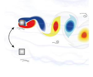
In this section, we recall the ROM proposed by Han et al. (Reference Han, Hémon, Pan and de Langre2021a). Considering a two-dimensional elastically supported square cylinder under flow, see figure 1(a), the cross-flow displacement  $Y$ satisfies a simple oscillator equation
 \begin{equation} m\ddot{Y}+c_s\dot{Y}+kY=F_{v}+F_{g}, \end{equation}
where  $m$ represents the total mass, including the mass
  $m_{s}$ of the body and the added mass
  $m_{a}$, and
  $c_{s}$ and
  $k$ represent the structural damping and stiffness, respectively. The added mass
  $m_{a}$ can be expressed as
  $m_{a} = C_{M}\rho D^{2}{\rm \pi} /4$ following Blevins (Reference Blevins2001), where
  $C_{M}$,
  $\rho$ and
  $D$ are the added mass coefficient, fluid density and the edge length of the square, respectively. In (2.1), (
  $\dot {}$ ) denotes the time derivation. The right-hand force term includes the lift force related to the unsteady vortex shedding
  $F_{v}$ and the galloping force
  $F_{g}$. Following Facchinetti, de Langre & Biolley (Reference Facchinetti, de Langre and Biolley2004), the vortex force
  $F_{v}$ can be expressed as
 \begin{equation} F_{v}=\rho U^2D C_{L}^{v}/2 = \rho U^2Dq C_{L0}/4, \end{equation}
where  $U$ is the incoming flow velocity and
  $C_{L0}$ represents the unsteady lift coefficient over a fixed cylinder. The parameter
  $q/2$ can be interpreted as a reduced vortex (or ‘fluctuating’) lift coefficient that represents the ratio between the unsteady vortex-induced lift coefficient of an oscillating cylinder
  $C_{L}^{v}$ and that of a fixed one
  $C_{L0}$. The dimensionless wake variable
  $q$ therefore directly determines the unsteady lift coefficient caused by vortex shedding, which can be modelled by a van der Pol nonlinear wake oscillator equation, coupled to the displacement
  $Y$
$Y$
 \begin{equation} \ddot{q}+\varepsilon\omega_f\left(q^2-1\right)\dot{q}+\omega_f^2q=(B_{1}/D)\ddot{Y}+\omega_f(B_{2}/D)\dot{Y}. \end{equation}
Here,  $\omega _{f}$ is the vortex-shedding angular frequency defined as
  $2{\rm \pi} S_{t}U/D$, where
  $S_{t}$ is the Strouhal number for flow over a stationary cylinder. In this equation,
  $\varepsilon =0.3$,
  $B_{1}=10$ and
  $B_{2}=0.1$ are constant coefficients derived from experimental data, see Han et al. (Reference Han, Hémon, Pan and de Langre2021a), and Appendix A for more details on the derivation of these values. The left-hand side of (2.3) is a van der Pol equation with a reference frequency
  $\omega _{f}$ and a growth rate
  $\varepsilon$. It is able to represent a linearly unstable (or self-excited) oscillator at this frequency, as well as a self-limited oscillation near
  $q=2$ (Nayfeh Reference Nayfeh2011). As such, it was found to be well adapted to model the oscillating lift force mentioned above (Facchinetti et al. Reference Facchinetti, de Langre and Biolley2004; Zanganeh & Srinil Reference Zanganeh and Srinil2016). The right-hand side forcing term of this equation expresses the influence of the solid motion on the wake dynamics. We use here the more general form where both the solid velocity and the solid acceleration have an influence: this was shown in Han et al. (Reference Han, Hémon, Pan and de Langre2021a) to be necessary for modelling VIV of square cylinders.

Figure 1. Elastically supported square cylinder under flow, with a representation of the wake oscillator variable  $q(t)$ and of the relative flow velocity that causes galloping.
The other force term in (2.1), the galloping force  $F_{g}$, is represented using the quasi-steady model of Parkinson & Smith (Reference Parkinson and Smith1964), see also Barrero-Gil et al. (Reference Barrero-Gil, Sanz-Andrés and Roura2009). We use a seventh-order polynomial, following the above references,
 \begin{equation} F_g=\frac{1}{2}\rho U^2D\cdot [A_1(\dot{Y}/U)-A_2(\dot{Y}/U)^3+A_3(\dot{Y}/U)^5-A_4(\dot{Y}/U)^7]. \end{equation}
 The main assumption of the classical quasi-steady theory is that the moving bluff body experiences the same instantaneous transverse force  $F_{g}$ as the stationary body which would be placed at the same incidence angle in a steady flow. Based on this, the galloping force in (2.4) depends on the solid cross-flow velocity through the ratio
  $(\dot {Y}/U)$, which is an approximation of the effective angle of attack of the flow,
  $\alpha$, see figure 1. The polynomial coefficients
  $A_{i}$ of the model are obtained by experiments or simulations from lift data of flow over a stationary square cylinder with varying angle of incidence. The first term of the polynomial in
  $(\dot {Y}/U)$ in (2.4), with a positive coefficient
  $A_{1}$, brings a negative damping force to the structural oscillator, leading to a linearly unstable galloping mode. The other higher-order terms have been introduced to model the rich behaviour in terms of a limit cycle with nonlinear geometrical effects. The coefficients
  $A_{i}$ will be further discussed in Appendix A.
We now introduce the dimensionless time  $t$, amplitude
  $y$, structural mass ratio
  $m_{s}^{*}$, total mass ratio
  $\mu$, structural angular frequency
  $\omega _s$, reduced velocity
  $U_{r}$, reduced angular frequency
  $\delta$ and damping ratio
  $\xi$, defined as
 \begin{equation} \left. \begin{gathered} t=T\omega_f, \quad y=Y/D, \quad m_{s}^{*}=m_s/\rho D^2, \quad \mu=(m_s+m_a)/\rho D^2, \\ \omega_s=\sqrt{k/m},\quad U_r=2{\rm \pi} U/(\omega_sD), \quad \delta=\omega_s/\omega_f=1/(S_{t}U_{r}), \quad \zeta=c_s/(2m\omega_s). \end{gathered} \right\} \end{equation}
 Substituting (2.4)(2.5) into (2.1)(2.3), yields the coupled equations governing the dynamics of the displacement  $y(t)$ and the wake variable
  $q(t)$
 \begin{gather} \ddot{y}+(2\zeta\delta)\dot{y}+\delta^{2} y \nonumber\\ =\dfrac{1}{8{\rm \pi}^{2}S_{t}^{2}\mu} \cdot \left\{\dfrac{qC_{L0}}{2}+[A_1(2{\rm \pi} S_{t}\dot{y})-A_2(2{\rm \pi} S_{t}\dot{y})^3+A_3(2{\rm \pi} S_{t}\dot{y})^5-A_4(2{\rm \pi} S_{t}\dot{y})^7]\right\}, \end{gather}
 \begin{gather} \ddot{q}+\varepsilon \left(q^2-1\right)\dot{q}+q=B_1\ddot{y}+B_2\dot{y}. \end{gather}
 This full nonlinear ROM will be further referred to as ROM-NL. Numerically solving the above two equations with a second-order finite difference scheme in time and an initial small perturbation in  $y$ results in a limit cycle on
  $y$ and
  $q$. The simplicity of this set of equations allows us to model the dynamics in an extremely low computational time, while reproducing quantitatively well the effect of the parameters (Han et al. Reference Han, Hémon, Pan and de Langre2021a).
2.2. LSA of the ROM
Following de Langre (Reference de Langre2006), Meliga & Chomaz (Reference Meliga and Chomaz2011), Zhang et al. (Reference Zhang, Li, Ye and Jiang2015), Navrose & Mittal (Reference Navrose and Mittal2016), Yao & Jaiman (Reference Yao and Jaiman2017), Li et al. (Reference Li, Lyu, Kou and Zhang2019) and Negi et al. (Reference Negi, Hanifi and Henningson2020), we also perform a LSA of the model given above in § 2.1. The linear version of the ROM, and the associated LSA will be referred to as ROM-LSA in the following, as opposed to ROM-NL which refers to the full nonlinear model. Removing all nonlinear terms in (2.6) and (2.7), there remains only
 \begin{gather} \ddot{y}+(2\zeta\delta)\dot{y}+\delta^{2} y= \dfrac{1}{8{\rm \pi}^{2}S_{t}^{2}\mu} \left(\dfrac{qC_{L0}}{2}+2{\rm \pi} A_1S_{t}\dot{y}\right), \end{gather}
 \begin{gather}\ddot{q}-\varepsilon \dot{q}+q=B_1\ddot{y}+B_2\dot{y}. \end{gather}
Assuming ( $y$,
$y$,  $q$)=(
 $y_{0}e^{\lambda t}$,
  $q_{0}e^{\lambda t}$) yields the frequency equation on
  $\lambda$
 $$\begin{gather} D(\lambda) = \lambda^{4} + \left(2\zeta\delta-\varepsilon-\dfrac{A_{1}}{4{\rm \pi} S_{t}\mu}\right) \lambda^{3} + \left( 1+ \dfrac{A_{1}\varepsilon}{4{\rm \pi} S_{t}\mu}-2\varepsilon \zeta\delta-\dfrac{B_{1}C_{L0}}{16{\rm \pi}^{2}S_{t}^{2}\mu}+\delta^{2} \right)\lambda^{2}\nonumber\\ + \left( 2\zeta\delta -\varepsilon \delta^{2}-\dfrac{A_{1}}{4{\rm \pi} S_{t}\mu}-\dfrac{B_{2}C_{L0}}{16{\rm \pi}^{2}S_{t}^{2}\mu} \right)\lambda+\delta^{2}=0. \end{gather}$$
 The roots of this fourth-order polynomial as a function of the dimensionless parameters give the ROM-LSA results, where the imaginary part, i.e.  $\lambda _{i}$, is the frequency, while the ratio of the real part to the imaginary part yields the normalized growth rate
  $G=\lambda _{r}/\lambda _{i}$. Note that we use here the normalized growth rate and not the growth rate
  $\lambda _{r}$ itself, for consistency with previous work on the topic (de Langre Reference de Langre2006; Violette et al. Reference Violette, de Langre and Szydlowski2010; Meliga & Chomaz Reference Meliga and Chomaz2011; Grouthier et al. Reference Grouthier, Michelin, Modarres-Sadeghi and de Langre2013). The polynomial has two pairs of conjugate solutions, of which only the roots with a positive imaginary part are of interest. For a given root, the ratio of the structural amplitude
  $y_{0}$ to the wake amplitude
  $q_{0}$ is obtained from (2.8) and (2.9)
 \begin{equation} \dfrac{y_{0}}{q_{0}} = \dfrac{\lambda^{2}-\lambda\varepsilon+1}{\lambda^{2} B_{1}+\lambda B_{2}} = \dfrac{C_{L0}}{16{\rm \pi}^{2}S_{t}^{2}\mu\left[ \lambda^{2} + \lambda\left( 2\zeta\delta-A_{1}/4 {\rm \pi}S_{t}\mu\right)+\delta^{2}\right]}. \end{equation}
 By letting the numerator equal zero, we can derive the root for the case where the square is fixed ( $y=0$), corresponding to a pure wake mode (PW)
 \begin{equation} \lambda_{PW} = \dfrac{\varepsilon \pm \sqrt{\varepsilon^2-4}}{2}, \quad G_{PW} = \frac{\varepsilon}{\sqrt{4-\varepsilon^2}}. \end{equation}
 This particular solution will be used to identify in the roots for the coupled problem, the mode where the dynamics is mainly in the wake variable  $q$. Conversely, the pure structural mode is defined by letting the denominator in (2.11) equal to zero.
The ROM-LSA will give two modes, as two degrees of freedom are involved. Three configurations may occur: (a) two stable modes, (b) one stable and one unstable and (c) two unstable modes. The first case is of little interest as no motion is expected. If only one mode is unstable we assume that the nonlinear response of the coupled system will occur following this mode. If the mode shape is dominant in  $q$ we shall label it as a wake mode (W) and conversely a solid mode (S) if dominant in
  $y$. When both modes are unstable, we assume, following Violette et al. (Reference Violette, de Langre and Szydlowski2010), that the most unstable one will eventually dominate the response.
2.3. Direct numerical simulations
For further validation, we also numerically solve the incompressible Navier–Stokes equations, coupled with a fluid–structure interaction solver, as in Han, Pan & Tian (Reference Han, Pan and Tian2018); Han et al. (Reference Han, Pan, Zhang, Wang and Tian2020). The entire computational domain is  $45D$ in length and
  $30D$ in width, split into several sub-regions to adopt the block dynamic mesh technique. In each sub-domain, structured grids are generated independently, with a total of 100 300 nodes. The distance between the first layer grid and the square surface is set to
  $0.005D$. For the boundary conditions, numerical scheme and the mesh generation strategy, see Han et al. (Reference Han, Pan, Zhang, Wang and Tian2020). The coupled structural motion is described by a classic mass–damper–stiffness (MCK) equation as (2.1), and solved with the second-order Newmark-beta method (Han et al. Reference Han, Huang, Pan, Wang, Zhang and Qin2021b). We set the time step at
  $\Delta t=0.01$, and apply 20 iterations in each step.
2.4. Validations
The ROM recalled above has already been validated against experimental data, for pure VIV, pure galloping and VIV–galloping interactions of a square cylinder in Han et al. (Reference Han, Hémon, Pan and de Langre2021a), showing good agreement between computed and experimental amplitudes of motion. Further validations are nevertheless needed as we apply the model here to investigate the low mass ratio behaviour at low Reynolds numbers. For this purpose, we consider the data from Zhao, Cheng & Zhou (Reference Zhao, Cheng and Zhou2013), Bhatt & Alam (Reference Bhatt and Alam2018) and Li et al. (Reference Li, Lyu, Kou and Zhang2019) who performed DNS to compute the motion of a square cylinder at  $Re=100$, with a small mass ratio of
  $m_{s}^{*}=3$ and a zero damping ratio
  $\zeta =0$. We use here a reduced velocity defined with the structural frequency in vacuum as in Zhao et al. (Reference Zhao, Cheng and Zhou2013), Bhatt & Alam (Reference Bhatt and Alam2018) and Li et al. (Reference Li, Lyu, Kou and Zhang2019). Our DNS and our ROM-NL model are applied to this case. The added mass coefficient is set to its standard value for a square using potential flow theory,
  $C_{M}=1.51$, see Blevins (Reference Blevins2001) and Pettigrew, Taylor & Kim (Reference Pettigrew, Taylor and Kim1989). Note that this differs from the value of 3.3 given in Li et al. (Reference Li, Lyu, Kou and Zhang2019) at
  $Re=100$ and 3.5 given in Joly et al. (Reference Joly, Etienne and Pelletier2012) at
  $Re=200$, which were those of their effective added mass coefficient, not the added mass coefficient. A discussion on the difference between these two forms of added mass coefficient and their use in our ROM can be found in Facchinetti et al. (Reference Facchinetti, de Langre and Biolley2004). The lift coefficient
  $C_{L0}=0.24$ and Strouhal number
  $S_{t}=0.15$ are taken from Bhatt & Alam (Reference Bhatt and Alam2018). The polynomial coefficients
  $A_{1}=-0.98$ and
  $A_{2}=14.4$ are taken from Joly et al. (Reference Joly, Etienne and Pelletier2012). Figure 2 shows the comparison between the models used in the present paper and the reference DNS cited above. A fast Fourier transformation (FFT) analysis of the displacement obtained by ROM-NL and DNS yields the dominant frequency
  $f_{osc}$. In, figure 2(b), the dimensionless frequency
  $f_{vac}^{*}$ is defined as the ratio of oscillation frequency
  $f_{osc}$ to the natural frequency in vacuum
  $2{\rm \pi} \sqrt {k/m_{s}}$. The results indicate that the present ROM can capture the important variations with the flow velocity at low Reynolds number and mass ratio. In addition, our DNS results show very good agreement with the other DNS data.

Figure 2. (a) Amplitude and (b) frequency of motion of an elastically supported square cylinder under flow as a function of the dimensionless flow velocity. Comparison between the models used in the paper (nonlinear ROM and DNS) and other DNS results (Zhao et al. Reference Zhao, Cheng and Zhou2013; Bhatt & Alam Reference Bhatt and Alam2018; Li et al. Reference Li, Lyu, Kou and Zhang2019). Dimensionless parameters:  $Re=100$;
  $m_{s}^{*}=3$;
  $\zeta =0$.
As mentioned in the Introduction, Joly et al. (Reference Joly, Etienne and Pelletier2012) reported a specific low mass ratio behaviour for a square cylinder under flow, at a reduced velocity of  $U_{r}=40$. Figure 3(a) shows the comparison between our results using ROM-NL and DNS and those taken from Joly et al. (Reference Joly, Etienne and Pelletier2012). The data obtained by Joly et al. (Reference Joly, Etienne and Pelletier2012) using DNS showed a strong decrease of amplitude at low mass ratios, while at high mass ratios their results converged to their quasi-steady model solution, which corresponds to (2.1) using only the quasi-steady force model, (2.4). Using the same parameters, the results with our ROM-NL give the same behaviour both quantitatively and qualitatively. The results of our DNS simulation also show the same evolution. This confirms that both our ROM-NL and DNS can capture the effects of mass ratio on amplitude, which is the object of present paper.

Figure 3. (a) Mass ratio effect on the amplitude of motion of a square cylinder under flow. The results of both our ROM-NL and DNS are compared with those of Joly et al. (Reference Joly, Etienne and Pelletier2012). (b) Magnitude of the vortex-induced lift as defined by Joly et al. (Reference Joly, Etienne and Pelletier2012). Comparison between the value fitted by Joly et al. (Reference Joly, Etienne and Pelletier2012) on their DNS results and that resulting from our ROM-NL. Dimensionless parameters:  $Re=200$;
  $\zeta =0$.
Joly et al. (Reference Joly, Etienne and Pelletier2012) also used a ROM in comparison with their results. It differs from our ROM-NL by the model of the vortex  $F_{v}$ which they defined by an amplitude
  $F_{0}$ and a time oscillation at the Strouhal frequency. They fit the amplitude
  $F_{0}$ to their DNS result yielding
  $F_{0}=0.66$. In our model, the amplitude of the vortex force needs not to be fitted but results from the computation of the limit cycle in
  $q(t)$ and is given by
 \begin{equation} F_{0}=\dfrac{q_{max}-q_{min}}{4}C_{L0}. \end{equation}
Figure 3(b) shows that our ROM-NL gives a good approximation of the vortex lift magnitude, without any fit.
The validations represented in figures 2, 3(a), and 3(b), where our ROM-NL is compared with existing DNS results, show that the model is able to qualitatively and in some aspects quantitatively represent several aspects of VIV and galloping of a square cylinder, even at low mass ratio and low Reynolds number. This confirms and widens the validation obtained in Han et al. (Reference Han, Hémon, Pan and de Langre2021a). In fact, more accurate fits with the DNS results can probably be obtained if the coefficients used in our ROM-NL were modified. This would not be illegitimate as, for instance, the lift coefficient  $C_{L0}$ and Strouhal numbers
  $S_{t}$ at
  $Re=200$ have been found to be in the range of 0.45–0.78 and 0.151–0.172, respectively, depending on the authors (Singh et al. Reference Singh, De, Carpenter, Eswaran and Muralidhar2009; Joly et al. Reference Joly, Etienne and Pelletier2012; Bhatt & Alam Reference Bhatt and Alam2018). A sensitivity analysis on these parameters is given in Appendix B. For the sake of consistency we have chosen to use for the subsequent analysis the same parameters as in Joly et al. (Reference Joly, Etienne and Pelletier2012):
  $C_{L0}=0.59$,
  $S_{t}=0.151$,
  $C_{M}=1.51$,
  $A_{1}=1.45$ and
  $A_{2}=79.44$. In the following, we take advantage of the simplicity of the ROM, both in its nonlinear (ROM-NL) and linearized (ROM-LSA) forms, to derive results in large ranges of flow velocity, mass and damping ratio.
2.5. Linear and nonlinear models and comparison with DNS
In the following, we seek to establish that the LSA of the ROM, referred to as ROM-LSA and defined in § 2.2, can effectively be used to describe the nonlinear behaviour predicted by ROM-NL and DNS in combined VIV and galloping of the square cylinder. It has been shown in Mannini, Massai & Marra (Reference Mannini, Massai and Marra2018) and Han et al. (Reference Han, Hémon, Pan and de Langre2021a) that, depending on the damping of the system, VIV and galloping may occur in separate ranges of flow velocity or in overlapping ranges, in which case they are said to be ‘coupled.’ The criterion to distinguish these two cases is based on the comparison between the critical reduced velocity for galloping,  $U_{g}$, and the resonance velocity for VIV,
  $U_{v}$. These two velocities can be derived from (2.8) and (2.9). At
  $U_{g}$ the linearized galloping force balances the structural damping, and at
  $U_{v}$ the frequencies of the two oscillator equations are equal. They read respectively
 \begin{equation} U_{g}=8{\rm \pi} \mu\zeta/A_{1}, \quad U_{v}=1/S_{t}. \end{equation}
 The ratio between them only depends on  $S_{t}$,
  $A_{1}$ and a combined mass–damping parameter generally referred to as the Scruton number
  $S_{c}^{*}$ which includes here the added mass
 \begin{equation} U_{g}/U_{v}=2S_{t}S_{c}^{*}/A_{1}, \quad S_{c}^{*}=4{\rm \pi}\mu\zeta. \end{equation}
 We consider a high mass ratio case,  $\mu =100$, with
  $S_{c}^{*}$ being equal to 5, 15 and 30. Note that we use here the total mass ratio
  $\mu$ as a variable rather than
  $m_{s}^{*}$, (2.5), because it is directly a coefficient of the ROM, (2.6). The limit cycle in amplitude of a heavy body undergoing VIV–galloping motion has been relatively well understood (Parkinson & Smith Reference Parkinson and Smith1964; Barrero-Gil et al. Reference Barrero-Gil, Sanz-Andrés and Roura2009; Mannini et al. Reference Mannini, Massai and Marra2018; Han et al. Reference Han, Hémon, Pan and de Langre2021a), and therefore it becomes a good candidate to verify whether the present linear model can explain the instabilities and show the mechanisms of VIV–galloping interaction. The selected
  $S_{c}^{*}$ numbers (5, 15 and 30) correspond to
  $U_{g}/U_{v}=1.04$, 3.12 and 6.25, which include both the coupled and separate VIV–galloping cases. In figure 4(a,c,e) the amplitude of the limit cycle in terms of displacement, obtained by the ROM-NL, is plotted as a function of the reduced velocity for the three values of
  $S_{c}^{*}$. The corresponding results of the ROM-LSA are plotted in figure 4(b,d,f), in terms of growth rates which are the roots of (2.10). One root can be attributed to a wake mode (W) by its proximity to the pure wake mode (PW) in (2.12a,b). The other one is referred to as the solid mode (S). Note that in our linearized model, (2.12a,b), the PW mode is always unstable, as will the W mode be. This means that a wake instability will always develop on
  $q$.
$q$.

Figure 4. Effect of the mass–damping parameter  $S_{c}^{*}$ on the amplitude of response
  $\hat {y}$ obtained by ROM-NL and DNS, and on the growth rates
  $G$ of the modes obtained by ROM-LSA, as a function of the reduced velocity. Dimensionless parameter: total mass ratio
  $\mu =100$; structural mass ratio
  $m_{s}^{*}=98.8$.
At  $S_{c}^{*}=30$, the ROM-LSA predicts an unstable solid mode at
  $U_{r}=40.8$, which is consistent with galloping starting at
  $U_{r}=40$ by the ROM-NL. VIV is seen in the ROM-NL by a peak of amplitude near
  $U_{r}=7$, corresponding well to the peak in growth rate of the wake mode in the ROM-LSA. When the Scruton number is set to 15, figure 4(c,d), galloping and VIV get closer in ranges, but the scenario is identical. At
  $S_{c}^{*}=5$, the separation between the two mechanisms of interaction is not so strong. In fact,
  $S_{c}^{*}=5$ corresponds to
  $U_{g}/U_{v}=1.04$, which means that VIV and galloping are expected to occur almost at the same velocity. In the ROM-NL result, it is found that galloping actually starts just after VIV is ended. This is also seen in the ROM-LSA, where the S mode is unstable only at
  $U_{r}=11.6$. Such a delay in the onset of galloping caused by the interaction with VIV was also observed by Parkinson & Wawzonek (Reference Parkinson and Wawzonek1981). From these results we see that the ROM-LSA allows us to describe with some accuracy the appearance of VIV and galloping, and their interactions.
For further comparison, we show some results using our DNS model in figure 4(c,e) for coupled and separate VIV–galloping motions, at  $S_{c}^{*}=5$ and
  $S_{c}^{*}=15$, respectively. Clearly, the ROM-NL and the ROM-LSA models give predictions that are consistent with DNS results. We also plot the corresponding oscillation frequencies obtained by ROM-NL, ROM-LSA and DNS in figure 5. For ROM-LSA, we consider the imaginary part of the roots of (2.10) and plot that of the solid mode (S) when unstable, and that of the wake mode (W) otherwise, consistently with figure 4(b,d,f). A dimensionless ratio
  $f^{*}$ of frequency
  $f_{osc}$ to the natural frequency
  $f_{s}=\omega _s/2{\rm \pi}$ is used. Figure 5 shows reasonable agreement between frequencies obtained by our ROM-NL, ROM-LSA and DNS models.

Figure 5. Comparisons of frequency of response obtained by ROM-NL, ROM-LSA and DNS, as a function of the reduced velocity, at (a)  $S_{c}^{*}=5$ for coupled and (b)
  $S_{c}^{*}=15$ for separate VIV–galloping motion.
3. Results
We may now use the models presented above to study the questions raised in the Introduction on the existence of a critical mass ratio for galloping and on the potential influence of damping on the answer. We focus on two particular configurations, separate VIV–galloping at  $S_{c}^{*}=15$ (corresponding to
  $U_{g}/U_{v}=3.12$) and coupled VIV–galloping at
  $S_{c}^{*}=5$ (corresponding to
  $U_{g}/U_{v}=1.04$). We use the ROM-NL, as above, to compute the amplitude
  $\hat {y}$, for a reduced velocity varying from 1 to 45. We consider low and high values of the total mass ratio
  $\mu =5$ and
  $\mu =500$, and recall the results for
  $\mu =100$ already given in figure 4. The responses for the two configurations, separate and coupled, are given in figures 6(a) and 6(b), respectively. The amplitudes for the large mass ratios,
  $\mu =100$ and 500, are almost identical in the two configurations. This is consistent with the results obtained at high
  $U_{r}$ by Jayatunga et al. (Reference Jayatunga, Tan and Leontini2015) using only the quasi-steady model for galloping and shows that the vortex force
  $F_{v}$ does not contribute to the response at high reduced velocity with large mass ratios.

Figure 6. Effect of mass ratio  $\mu$ and of mass–damping parameter
  $S_{c}^{*}$ on the amplitude of response
  $\hat {y}$ and on the growth rates
  $G$ of modes obtained by ROM-LSA, as a function of the reduced velocity. (a,c,e) High damping,
  $S_{c}^{*}=15$ corresponding to separate VIV and galloping. (b,d,f) Low damping,
  $S_{c}^{*}=5$, corresponding to coupled VIV and galloping. Top line, amplitude of response using the ROM-NL and DNS. Middle and bottom lines growth rates of modes for large and small mass ratios, respectively. Dimensionless parameter: total mass ratio
  $\mu =5$, 100 and 500; structural mass ratio
  $m_{s}^{*}=3.8$, 98.8 and 498.8.
The amplitude of motion is quite different at low mass ratios in the two configurations. The VIV range is extended, and galloping is delayed to larger velocities when compared with the responses for higher mass ratios. Moreover, figure 6(a) shows that a high  $S_{c}^{*}$ will further widen the VIV range and delay galloping. DNS results in figure 6(a,b) support our results obtained by ROMs.
These results lead us to investigate the relation between the delay in the onset of galloping and the apparent extension of the range of VIV in this low mass ratio range. We use the linear stability analysis (ROM-LSA), focusing first on the configuration of large  $S_{c}^{*}$ where VIV and galloping are well separated at high mass ratios.
3.1. Low mass ratio behaviour in the case of separate VIV and galloping
Figure 6(c,e) shows the ROM-LSA results at large  $S_{c}^{*}=15$, with a high (
 $\mu =100$) and a low (
 $\mu =5$) mass ratio, respectively. Contrary to the high mass cases, in the ROM-NL response for
  $\mu =5$, figure 6(a), a large range of VIV was observed, with delayed galloping. This phenomenon can be now interpreted through the ROM-LSA results in figure 6(e). The growth rate for the wake mode is still larger than
  $G_{pw}$ in a large range of velocity, indicating that the wake instability is enhanced by the presence of a solid mode close to instability. In addition, since the solid mode becomes unstable only above
  $U_{r}=22.5$, we can state that the motion below this critical value is induced exclusively by the wake instability. Moreover, in this case, the square cylinder does not start galloping immediately when the solid mode becomes unstable. This is because, see figure 6(e), there is a range after
  $U_{r}=22.5$, where not only is the growth rate for the solid mode positive, but also the wake mode is larger than
  $G_{pw}$, and both are unstable. In this range, a competition exists between VIV and galloping. First, just above
  $U_{r}=22.5$, the wake mode is still sufficiently unstable to overcome the unstable solid mode, which explains why VIV still occurs. At larger velocities, the growth rate of the solid mode keeps increasing and eventually dominates. The motion switches to galloping, but the onset has been delayed. As shown here by the ROM-LSA, the delay in galloping is caused by the presence of extended VIV. The range of flow velocity where VIV occurs is extended because of the total damping level which is reduced by the effect of the galloping forces.
3.2. Low mass ratio behaviour in the case of coupled VIV and galloping
For the more complex configuration of coupled VIV and galloping, we now apply the same approach. We show the ROM-LSA results for  $S_{c}^{*}=5$ with high
  $\mu =100$ and low
  $\mu =5$ mass ratios, respectively in figure 6(d,f). For the low mass ratio case, figure 6(f), a scenario comparable to figure 6(e) is found, with a competition between the wake mode instability, giving VIV, and the solid mode instability, giving galloping. This results also in a delayed galloping. Still, a significant difference can be seen with the configuration analysed above where VIV and galloping were well separated: here, the wake mode is still largely unstable when the solid mode becomes unstable. This results in a higher VIV response, and therefore an extended VIV domain. Note that, in figure 6(b), the amplitude variation in the grey area is caused by the 3:1 synchronization between the vortex-shedding frequency and the oscillation frequency of the body (Zhao et al. Reference Zhao, Leontini, Lo Jacono and Sheridan2014).
3.3. No critical mass ratio for galloping
We have just seen that, even though a low mass ratio does enhance the wake instability that causes VIV, the solid mode involved in galloping always becomes unstable at higher flow velocities. More importantly, as the reduced velocity  $U_{r}$ is increased, the growth rate for the solid mode keeps increasing whereas the growth rate for the wake mode approaches
  $G_{pw}$ continuously, see figure 6(c–f). We now state that, in a more general case, the solid mode giving galloping will always, at high reduced velocity, become more unstable than the wake mode giving VIV. Therefore, although galloping can be delayed at low mass ratio, by the mechanism shown above of mode competition, it will not disappear. The concept of a critical mass ratio below which galloping does not exist is therefore not appropriate: there is no critical mass ratio but simply a delay effect. Moreover, our results show that the domain of reduced velocity where VIV occurs can be extended at low mass ratio, but that the corresponding growth rate always decreases for higher velocities. We state that ‘VIV forever’, which was thought to be related to the suppression of galloping, see Li et al. (Reference Li, Lyu, Kou and Zhang2019), Sourav & Sen (Reference Sourav and Sen2020), actually does not occur here.
We now use our DNS model to confirm whether galloping can actually be found, for low mass ratios, at higher reduced velocities. Figure 7(a) shows that, even at a mass ratio of  $m_{s}^{*}=2$, a high amplitude of motion can be found provided the reduced velocity is increased up to
  $U_{r}=90$. To confirm that this motion is caused by galloping, we show in figure 7(b) the evolution in time of the response at
  $U_{r}=66$ and at
  $U_{r}=98$. At
  $U_{r}=98$ the motion is of larger amplitude and a much lower frequency than at
  $U_{r}=66$. In fact the oscillation frequency,
  $f_{osc}$, is close to that of the MCK oscillator without flow,
  $f_{s}$. A FFT analysis of the response yields a frequency such that
  $f_{osc}/f_{s}=0.7$. Large amplitudes and low frequencies are typical signs of galloping (Blevins Reference Blevins2001; Nemes et al. Reference Nemes, Zhao, Lo Jacono and Sheridan2012; Li et al. Reference Li, Lyu, Kou and Zhang2019). To further support our conclusion that galloping is just delayed at a very low mass ratio, we show the amplitude
  $\hat {y}$ and frequency
  $f^{*}$ responses via DNS at a low mass ratio
  $m_{s}^{*}=2$ with a wide range of
  $U_{r}$ in figures 7(c) and 7(d), respectively. The parameters used are the same as in figure 3(a) of Joly et al. (Reference Joly, Etienne and Pelletier2012). For comparison, the case of high mass ratio
  $m_{s}^{*}=20$ is also added. Figure 7(c) shows that the increased amplitude corresponding to galloping is delayed at low mass ratio. Consistently, in figure 7(d), the drop from the VIV frequency to the lower galloping frequency does occur at high reduced velocity for this low mass ratio. We can therefore confirm by DNS that galloping can be found even at a low mass ratio, but at high reduced velocities.

Figure 7. (a) Effect of mass ratio on the amplitude of motion of a square cylinder. The results of Joly et al. (Reference Joly, Etienne and Pelletier2012) and our ROM-NL and DNS at  $U_{r}=40$ are those already given in figure 3(a). Our DNS results at
  $U_{r}=66$ and
  $U_{r}=90$ show that there exists a transition to galloping at low mass ratio. (b) Time histories of the displacement at
  $U_{r}=66$ and
  $U_{r}=98$, at
  $m_{s}^{*}=2$, showing a VIV response and a galloping response, respectively. Panels (c,d) are respectively the amplitude
  $\hat {y}$ and the frequency
  $f^{*}$ of a square cylinder for a high
  $m_{s}^{*}=20$ and low
  $m_{s}^{*}=2$ mass ratios, as a function of the reduced velocity
  $U_{r}$.
4. Discussions and conclusions
In the present work we have used both the original nonlinear ROM for VIV and galloping (ROM-NL) and its linearized version in view of a LSA (ROM-LSA). Consistently with previous work on VIV (Violette et al. Reference Violette, de Langre and Szydlowski2010; Grouthier et al. Reference Grouthier, Michelin, Modarres-Sadeghi and de Langre2013) we found that the use of ROM-LSA is relevant to the prediction of some aspects of the dynamics of the limit cycle that arise in the nonlinear system. The frequency of motion, figure 5, is generally well predicted. This is related to the fact that the linearly most unstable mode in most cases remains the dominant mode in the limit cycle, as can be seen in figures 4 and 6. Nevertheless, when two modes are unstable with comparable growth rates, such as for instance in figure 6(e) in the range  $U_{r}=30{-}40$, nonlinear effects influence the competition between modes: the ROM-LSA predicts a cross-over between VIV and galloping at
  $U_{r}=33.1$, figure 6(e), whereas it is observed later, at
  $U_{r}=36.9$, with the ROM-NL, figure 6(a). Because of its simplicity, the ROM-LSA can therefore be considered as a useful tool for the qualitative and quantitative prediction of combined VIV and galloping. Moreover, as most of the results on vibration responses we gave using ROM-NL have been confirmed by DNS, see figures 2–7, both the linear and the nonlinear versions of the ROM can be considered as reliable.
The particular effect of damping in the mechanisms presented above needs now to be discussed. In most systems under VIV, increasing the damping of the structure reduces the range of flow velocity where motion occurs (Païdoussis et al. Reference Païdoussis, Price and de Langre2010). Conversely, in the present case of very low mass ratios, the VIV range is indeed increased by damping, as can be seen by comparing figure 6 panels (a) and (b), where  $S_{c}^{*}$ is respectively 15 and 5 and where the range of lock-in is larger in the first case. This is consistent with Sourav & Sen (Reference Sourav and Sen2019), where the responses of damped and undamped square cylinders were compared. Here, we have related this particular effect of damping to the competition in the evolution of the growth rates of the wake and solid modes. The enlarged VIV range corresponded to a dominant wake mode, under the influence of the solid mode. Here, an increase of the damping ratio results in a delay of the instability by galloping of the solid mode: as a consequence, the only unstable mode left in that range is the enhanced wake, resulting in VIV. To summarize, at low mass ratio and high damping, VIV is allowed to extend by the delay of galloping. This is of importance when considering the possible use of square cross-sections to harvest energy from flow, using their cross-flow motion: the low mass ratio configuration is favourable to energy harvesting because (a) there is always motion, either by VIV or by galloping and (b) damping, or equivalently energy extraction, does not reduce the range of flow velocity where motion is found.
Our results can also be used to give some insights into the range of applicability of (2.14a,b), i.e. the classical quasi-steady model, which is generally used to derive the critical flow velocity where galloping starts. The quasi-steady model is generally considered to be valid at high reduced velocity  $U_{r}$, where the incoming velocity
  $U$ is much larger than the vibration velocity
  $\dot {Y}$. In addition, as (2.14a,b) assumes that the only destabilizing force is the galloping force, it ignores the possible interaction with VIV. Because of this interaction, the predicted onset of galloping by the quasi-steady model (2.14a,b) at large mass ratio and low
  $S_{c}^{*}$ number is less accurate than that at a high
  $S_{c}^{*}$ number, where VIV and galloping are well separated. In addition, we found here that at low mass ratio
  $\mu =5$ the prediction is actually inaccurate for both low and high
  $S_{c}^{*}$, even at a high reduced velocity:
  $U_{g}=20.69$ instead of approximately 36.9 at
  $S_{c}^{*}=15$, figure 6(a), and
  $U_{g}=6.89$ instead of approximately 18 at
  $S_{c}^{*}=5$, figure 6(b). This is due to the strong interaction between VIV and galloping, as discussed above. This shows that, for predicting oscillations of a square cylinder at low mass ratio, such as underwater flow, a combined VIV and galloping model is needed.
The analysis presented here considered a two-dimensional situation, which is generally used for these problems. The ROM, ROM-NL, (2.6) and (2.7) can also be extended to slender flexible or tensioned structures such as beams or cables (Violette, de Langre & Szydlowski Reference Violette, de Langre and Szydlowski2007; Païdoussis et al. Reference Païdoussis, Price and de Langre2010). Projecting the fluid forces onto the modes of the structures then reduces the problem to a system of equations similar to (2.6)–(2.7). We may therefore expect similar results in terms of the effect of the mass ratio on the existence of galloping.
Our main result on the existence of galloping even at low mass ratio is probably applicable to all cross-sections that experience galloping. In fact, our ROM, (2.6) and (2.7), can be applied to any cross-section provided the coefficients for the vortex force and for the galloping force are known. Sections prone to galloping such as rectangular or triangular ones will have different sets of coefficients, but the mechanism of VIV and galloping, and their interaction, is expected to be the same. Of course, for a section that is neutral to galloping (such as the circular cylinder) or stable to galloping (such as the rotated square cylinder), the issue is irrelevant, even if some low mass ratio effects exist on the wake mode instability (Yao & Jaiman Reference Yao and Jaiman2017). To explore the possibility that our conclusions are also valid for other cross-sections and at higher Reynolds numbers, we consider the case of a  $3:2$ rectangular cross-section. The experimental results of Mannini et al. (Reference Mannini, Massai, Marra and Bartoli2015, Reference Mannini, Massai and Marra2018) are shown in figure 8. As their mass ratio is high (
 $\mu =785.2$), the VIV and galloping responses are well separated. The Reynolds number varies in their experiment from 20 000 to 150 000. We first compute the response of our ROM-NL at this mass ratio, using
  $C_{M}=1.51$ from Blevins (Reference Blevins2001), the flow parameters (
 $S_{t}$,
  $C_{L0}$ and
  $A_{i}$) and structural parameters (
 $\zeta$,
  $S_{c}^{*}$) from Mannini et al. (Reference Mannini, Massai, Marra and Bartoli2015, Reference Mannini, Massai and Marra2018) and
  $B_{1}=10$,
  $B_{2}=0.1$ as in our previous computations on squares. As reported by Mannini et al. (Reference Mannini, Massai, Marra and Bartoli2015, Reference Mannini, Massai and Marra2018), among the tested
  $Re$ range in their experiments, the Strouhal number
  $S_{t}=0.106$ is almost not affected by the Reynolds number, while the lift coefficient
  $C_{L0}$ approximately varies from 0.659 to 1.113. We use here
  $C_{L0}=0.785$, which is the mean of the measured points in Mannini et al. (Reference Mannini, Massai and Marra2018). The quasi-steady polynomial coefficients
  $A_{i}$ are taken from the experiments in Mannini et al. (Reference Mannini, Massai, Marra and Bartoli2015) at
  $Re=146\,800$. The comparison with the experimental data, figure 8 shows a good agreement for this high mass ratio case. Decreasing now the mass ratio to
  $\mu =10$, without changing any other coefficients, we obtain with the ROM-NL a response that shows an extended range of VIV and a delayed galloping. This is very similar to our observations on the square section at low Reynolds number and confirms that the scenario we described for the square section at low Reynolds number probably applies for other sections and other Reynolds numbers.

Figure 8. Amplitude of motion of a  $3:2$ rectangular cylinder obtained by the present ROM-NL, as a function of the reduced velocity for two mass ratios. Comparison with the experimental data of Mannini et al. (Reference Mannini, Massai and Marra2018) for high mass ratio. The low mass ratio case shows extended VIV and delayed galloping, as for the square cylinder.
To summarize and conclude: we have addressed the two questions raised at the end of the Introduction on the existence of galloping at low mass ratio and on the role of damping in that range of parameters. We have shown that, contrary to the statements in several recent papers, there is no critical mass ratio for galloping of square cylinders under flow, regardless of damping.
Funding
This work was supported by the National Natural Science Foundation of China (NSFC grant no. 51879220).
Declaration of interests
The authors report no conflict of interest.
Appendix A. Estimations of parameters  $A_{i}$ and $B_{i}$ in ROM-NL


For completeness, this appendix aims to provide guidelines for the derivation of parameters used in the ROM-NL model. It summarizes elements from Han et al. (Reference Han, Hémon, Pan and de Langre2021a). For a given bluff body under a specific flow, the mass ratio  $\mu$ including the structural mass ratio
  $m_{s}^{*}$ and the added mass coefficient
  $C_{M}$, the damping ratio
  $\zeta$, the natural angular frequency
  $\omega _s$ and the reduced velocity
  $U_{r}$ are known. The Strouhal number
  $S_{t}$ and lift coefficient
  $C_{L0}$ can be determined by experiments or simulations of flow over a fixed bluff body.
As mentioned previously in § 2.1 and in (2.4), the parameters  $A_{i}$ coupled with
  $\dot {Y}/U$ (
 $\dot {Y}/U\approx \alpha$) are used to describe the incidence angle effects of the galloping force
  $F_{g}$ based on the quasi-steady theory. The values of
  $A_{i}$ can be estimated by simulations and experiments of flow over a fixed cylinder under different incidence angles. In this paper, the parameters are directly taken from Joly et al. (Reference Joly, Etienne and Pelletier2012) and Mannini et al. (Reference Mannini, Massai, Marra and Bartoli2015). For a square cylinder at low Reynolds numbers, Joly et al. (Reference Joly, Etienne and Pelletier2012) computed DNS data of the lift coefficient as a function of the incidence angle
  $\alpha$, and they used a third-order polynomial including
  $A_{1}$ and
  $A_{2}$ to fit their numerical data, giving
  $A_{1}=-0.98$ and
  $A_{2}=14.4$ at
  $Re=100$ and
  $A_{1}=1.45$ and
  $A_{2}=79.44$ at
  $Re=200$. In figure 8, for a
  $3:2$ rectangular cylinder at high-
 $Re$ flow, Mannini et al. (Reference Mannini, Massai, Marra and Bartoli2015) conducted experiments at
  $Re=146\,800$ of flow over the fixed rectangular cylinder with varying angles
  $\alpha$ from
  $0^{\circ }$ to
  $16^{\circ }$. An eleventh-order polynomial was used by (Mannini et al. Reference Mannini, Massai, Marra and Bartoli2015, Reference Mannini, Massai and Marra2018) to fit the experimental data, resulting in
  $A_{1}=5.5$,
  $A_{2}=318.2$,
  $A_{3}=32\,150$,
  $A_{4}=1.231\times 10^{6}$,
  $A_{5}=1.798\times 10^{7}$,
  $A_{6}=8.977\times 10^{7}$.
The coupling parameters  $B_{1}$ and
  $B_{2}$ are estimated by forced vibration experiments of a square cylinder, see Han et al. (Reference Han, Hémon, Pan and de Langre2021a). Considering a forced vibration at the amplitude
  $y_0$ and forced frequency
  $\omega$, with a first harmonic approximation, yields
 \begin{equation} y=y_{0}cos(\omega t) \quad q=q_0cos(\omega t+\theta), \end{equation}
where  $\theta$ represents the phase angle between
  $q$ and the displacement
  $y$. Note that we define here the frequency
  $\omega$ scaled by the vortex-shedding frequency,
  $\omega _f$. First, substituting (A1a,b) into the wake oscillator (2.7) and considering only the main harmonic contribution of the nonlinearities gives
 \begin{gather} q_0^6-8q_0^4+16\left[1+\left(\dfrac{\omega^2-1}{\varepsilon\omega}\right)^2\right]q_0^2=16\left(\dfrac{B_1y_0\omega}{\varepsilon}\right)^2+16\left(\dfrac{B_2y_0}{\varepsilon}\right)^2, \end{gather}
 \begin{gather} \theta=\arctan \dfrac{\varepsilon\omega}{\omega^2-1}(q_0^2/4-1)+\arctan\dfrac{B_2\omega}{-B_1\omega^2}. \end{gather}
 Solving the bi-cubic polynomial in (A2), we can have the unique positive real root  $q_{0}$ and therefore the instantaneous lift coefficient caused by vortices
 \begin{equation} C_{L}^{v}=qC_{L0}/2=q_0C_{L0}\cos(\omega t+\theta)/2. \end{equation}
 Second, substituting (A1a,b) into the quasi-steady model (2.4) gives the galloping force  $F_{g}$ and its dimensionless force coefficient
  $C_{L}^{g}$, which reads
 $$\begin{gather} C_{L}^{g}=2F_{g}/\rho U^2D=\left[{-}2{\rm \pi} S_{t} y_0\omega A_1+(2{\rm \pi} S_{t} y_0\omega)^3 \frac{3}{4}A_2\right.\nonumber\\ \left.- (2{\rm \pi} S_{t}y_0\omega)^5 \frac{5}{8}A_3+(2{\rm \pi} S_{t}y_0\omega)^7 \frac{35}{64}A_4\right]\sin(\omega t). \end{gather}$$
 Now, the total lift coefficient  $C_{L}^{t}$ of a vibrating square cylinder can be built by
 \begin{equation} C_{L}^{t}=C_{L}^{v}+C_{L}^{g}-C_{L}^{a}, \end{equation}
where the coefficient  $C_{L}^{a}$ represents the added mass effects that can be computed by substituting (A1a,b) into
  $C_{L}^{a}=2m_{a}\ddot {Y}/\rho U^2D$
 \begin{equation} C_{L}^{a}={-}\omega^2 C_M2{\rm \pi}^3S_{t}^2y_0\cos(wt). \end{equation}
 Then, after elementary algebra by combining (A2)–(A7), the total lift coefficient can be given by a function as  $C_{L}^{t}=Rcos(\omega t+\varTheta )$, of which
  $R$ and
  $\varTheta$ can be expressed by
 \begin{gather} R^2=(0.5C_{L0}q_0cos\theta+\omega^2 C_M2{\rm \pi}^3S_{t}^2y_0)^2+\left[\vphantom{\frac{5}{8}}-0.5C_{L0}q_0sin\theta-2{\rm \pi} S_{t}y_0\omega A_1\right.\nonumber\\ \left.+(2{\rm \pi} S_{t}y_0\omega)^3\frac{3}{4}A_2-(2{\rm \pi} S_{t}y_0\omega)^5 \frac{5}{8}A_3+(2{\rm \pi} S_{t}y_0\omega)^7 \frac{35}{64}A_4\right]^2, \end{gather}
 \begin{gather} tan\varTheta=\left[{-}0.5C_{L0}q_0sin\theta-2{\rm \pi} S_{t}y_0\omega A_1+(2{\rm \pi} S_{t}y_0\omega)^3\frac{3}{4}A_2-(2{\rm \pi} S_{t}y_0\omega)^5 \frac{5}{8}A_3\right.\nonumber\\ \left.\left.+(2{\rm \pi} S_{t}y_0\omega)^7 \frac{35}{64}A_4\right]\right/(0.5C_{L0}q_0cos\theta+\omega^2 C_M2{\rm \pi}^3S_{t}^2y_0). \end{gather}
 Solving the above (A8) and (A9), the theoretical total lift coefficient amplitude,  $R$, and phase angle,
  $\varTheta$, can be obtained. Figure 9(a,b) shows the comparison of the theoretical predictions and experiments in terms of
  $R$ and
  $\varTheta$, respectively. Note that the reduced velocity for the forced vibrations is defined as
  $U_{r}=1/\omega S_{t}$. The coefficients
  $A_{1}=3.01$,
  $A_{2}=110$,
  $A_{3}=3037$ and
  $A_{4}=26\,515$ are estimated by Freda, Carassale & Piccardo (Reference Freda, Carassale and Piccardo2015) via experiments, while other parameters are taken from Carassale, Freda & Banfi (Reference Carassale, Freda and Banfi2015). The results indicate that
  $B_{1}=10$ and
  $B_{2}=0.1$ applied in the present work are reasonable to capture the most important features of a vibrating square cylinder under flow.

Figure 9. (a) Amplitude of lift coefficient,  $R$, and (b) phase angle,
  $\varTheta$, of a square cylinder under forced vibrations (
 $y_0=0.1$). Experimental data are taken from Carassale et al. (Reference Carassale, Freda and Banfi2015).
Appendix B. Sensitivity analysis of ROM-NL
The results obtained by our ROM-NL depend on the parameters in (2.6) and (2.7). The lift coefficient  $C_{L0}$ and the Strouhal number
  $S_{t}$ have values that are found to vary among sources. For instance, at
  $Re=200$,
  $C_{L0}$ is given in the range 0.45–0.78 and
  $S_{t}$ in the range 0.15–0.172 in Singh et al. (Reference Singh, De, Carpenter, Eswaran and Muralidhar2009), Joly et al. (Reference Joly, Etienne and Pelletier2012) and Bhatt & Alam (Reference Bhatt and Alam2018). For this reason we give a sensitivity analysis of
  $C_{L0}$ and
  $S_{t}$ for our ROM-NL in this appendix, in order to investigate whether the sensitivity is a possible cause of differences between ROM-NL and DNS in figure 3(a). Using the same parameters as figure 3(a), we plot comparisons of the amplitude
  $\hat {y}$ predicted by our ROM-NL and by DNS with different values of
  $C_{L0}$ and
  $S_{t}$ in figure 10. In the reasonable range of
  $C_{L0}$, a higher value of
  $C_{L0}$ will lower the minimum amplitude and increase the range of velocities for low amplitude vibrations. The Strouhal number will significantly affect the predictions among the resonance region around
  $U_{r}=1/S_{t}$, however, the reduced velocity
  $U_{r}=40$ here is quite large; the results obtained by ROM-NL are not sensitive to
  $S_{t}$. One might notice that
  $S_{t}$ indeed affects the oscillations in the curves below
  $M_{s}^{*}=5$. This phenomenon is the ‘kink’ similar to figure 6(b), which occurs for light bodies when the vortex-shedding frequency is in the vicinity of an odd-integer multiple of oscillation frequency (Zhao et al. Reference Zhao, Leontini, Lo Jacono and Sheridan2014). The value of
  $S_{t}$ determines the vortex-shedding frequency and therefore changes the predictions and the oscillations at a low mass ratio. In a word, reasonably optimal parameters could possibly be found by varying
  $C_{L0}$ and
  $S_{t}$ to improve the accuracy against the DNS data. In the present work, however, we did not use such a fit and all the parameters used in our ROMs are taken from Joly et al. (Reference Joly, Etienne and Pelletier2012) for consistency. More importantly, a different set of parameters will not change the mechanism of VIV–galloping behaviour obtained by our ROM-LSA, and the present set of parameters are already ‘accurate enough’ for our phenomenological and extremely-low-cost ROM.

Figure 10. A sensitivity analysis of the effects of the (a) lift coefficient,  $C_{L0}$, and (b) Strouhal number,
  $S_{t}$, on the amplitude response
  $\hat {y}$ obtained by ROM-NL.


