


1. Introduction
Starting from the seminal work of Nikuradse (Reference Nikuradse1931), turbulent flows over rough surfaces have been commonly studied in the presence of statistically homogeneous roughness. The drag penalty induced by the imperfections of the surface is reflected in a vertical shift of the universal logarithmic velocity profile, which can be readily calculated from the equivalent sand-grain roughness (see, for instance, the review by Chung et al. Reference Chung, Hutchins, Schultz and Flack2021). The equivalent roughness is in turn a hydraulic quantity whose a priori calculation from the roughness topology is the subject of ongoing research (e.g. Flack & Schultz Reference Flack and Schultz2010; Yang et al. Reference Yang, Stroh, Lee, Bagheri, Frohnapfel and Forooghi2023).
However, naturally occurring rough surfaces (such as that generated by the deposition of dirt, ice or organic matter over the surface of a vehicle) can rarely be regarded as homogeneous, so that the effect they have on the flow is more complex than a vertical shift of the velocity profile. For example, Mejia-Alvarez et al. (Reference Mejia-Alvarez, Barros, Christensen, Vendetti, Best, Church and Hardy2013) have inspected the roughness generated on a turbine blade by deposition of foreign materials, finding that it contained randomly distributed elements of different scales. The flow over such a multi-scale roughness has been experimentally investigated in a boundary layer wind tunnel (Mejia-Alvarez & Christensen Reference Mejia-Alvarez and Christensen2013; Barros & Christensen Reference Barros and Christensen2014). It has been found that the ensemble-averaged velocity field is highly heterogeneous as it contains coherent regions of low and high momentum (low and high momentum pathways); these occur in the absence of obvious geometric features (e.g. ridges). As a note of caution, it is worth highlighting that the rough surface used in the mentioned studies was manufactured by aligning several identical rough plates; this creates a large-scale regularity in the surface that might favour the formation and sustainment of the observed momentum pathways. The pathways have an
 $h$
-scaled extent in the streamwise and wall-normal direction, where
$h$
-scaled extent in the streamwise and wall-normal direction, where
 $h$
is the outer length scale (the boundary layer thickness for the studies mentioned here). Nikora et al. (Reference Nikora, Stoesser, Cameron, Stewart, Papadopoulos, Ouro, McSherry, Zampiron, Marusic and Falconer2019) observed similar coherent motions over multi-scale roughness in open channel flows, finding that the pathways provide a contribution to skin friction that adds up to the direct effect of roughness. Comparable low- and high-momentum pathways were found both experimentally (Womack et al. Reference Womack, Volino, Meneveau and Schultz2022) and numerically (Kaminaris et al. Reference Kaminaris, Balaras, Schultz and Volino2023) by studying the turbulent flow over a random distribution of truncated conical roughness elements resembling the barnacles that accumulate on ship hulls. These pathways extend for at least
$h$
is the outer length scale (the boundary layer thickness for the studies mentioned here). Nikora et al. (Reference Nikora, Stoesser, Cameron, Stewart, Papadopoulos, Ouro, McSherry, Zampiron, Marusic and Falconer2019) observed similar coherent motions over multi-scale roughness in open channel flows, finding that the pathways provide a contribution to skin friction that adds up to the direct effect of roughness. Comparable low- and high-momentum pathways were found both experimentally (Womack et al. Reference Womack, Volino, Meneveau and Schultz2022) and numerically (Kaminaris et al. Reference Kaminaris, Balaras, Schultz and Volino2023) by studying the turbulent flow over a random distribution of truncated conical roughness elements resembling the barnacles that accumulate on ship hulls. These pathways extend for at least
 $18h$
(Womack et al. Reference Womack, Volino, Meneveau and Schultz2022) in the streamwise direction; the position at which they occur is reproducible across different repetitions of the same experiment. Also, high- and low- momentum pathways of an
$18h$
(Womack et al. Reference Womack, Volino, Meneveau and Schultz2022) in the streamwise direction; the position at which they occur is reproducible across different repetitions of the same experiment. Also, high- and low- momentum pathways of an
 $h$
-scaled spanwise period were observed by Reynolds et al. (Reference Reynolds, Hayden, Castro and Robins2007) in a boundary layer evolving over an array of staggered cubic roughness elements. In this last case, however, the spanwise period of the momentum pattern increased with streamwise fetch in an almost quantised manner.
$h$
-scaled spanwise period were observed by Reynolds et al. (Reference Reynolds, Hayden, Castro and Robins2007) in a boundary layer evolving over an array of staggered cubic roughness elements. In this last case, however, the spanwise period of the momentum pattern increased with streamwise fetch in an almost quantised manner.
There is no consensus over what triggers the formation of these momentum pathways. Kaminaris et al. (Reference Kaminaris, Balaras, Schultz and Volino2023) found that the spanwise topology of the pathways correlates well with that of the leading edge of the roughness (that is, the first row of roughness elements stretching over the spanwise direction). They went on to show that the pathways are effectively triggered by the leading edge, and persist for a finite distance downstream of it regardless of whether they evolve over a smooth or a rough surface. Conversely, Barros & Christensen (Reference Barros and Christensen2014) found a local correlation between the roughness topology and the pathways, suggesting that the pathways originate from heterogeneity in the roughness properties in a similar way to secondary motions over spanwise heterogeneous roughness. It is unclear which of these two mechanisms is dominant; it cannot be excluded that both contribute to the formation of the pathways. Nevertheless, there is a close resemblance between the pathways and secondary motions observed over spanwise heterogeneous roughness (as we will discuss below), to the point that the pathways themselves are also referred to as secondary motions. Both the pathways and the secondary motions, in turn, have often been linked to the naturally occurring very-large-scale motions (VLSMs; see, for instance, Kim & Adrian Reference Kim and Adrian1999; Hutchins & Marusic Reference Hutchins and Marusic2007a ; Lee & Moser Reference Lee and Moser2018) seen in turbulent wall-bounded flows.
Spanwise heterogeneous roughness is usually studied in terms of spanwise-alternating streamwise-elongated strips with different roughness properties (Hinze Reference Hinze1967; Nugroho et al. Reference Nugroho, Hutchins and Monty2013; Turk et al. Reference Türk, Daschiel, Stroh, Hasegawa and Frohnapfel2014; Willingham et al. Reference Willingham, Anderson, Christensen and Barros2014; Anderson et al. Reference Anderson, Barros, Christensen and Awasthi2015; Stroh et al. Reference Stroh, Hasegawa, Kriegseis and Frohnapfel2016; Vanderwel et al. Reference Vanderwel, Stroh, Kriegseis, Frohnapfel and Ganapathisubramani2019; Stroh et al. Reference Stroh, Schäfer, Frohnapfel and Forooghi2020; Frohnapfel et al. Reference Frohnapfel, Von Deyn, Yang, Neuhauser, Stroh, Örlü and Gatti2024). The strip width is typically indicated by
 $s$
; notice that this is half the period
$s$
; notice that this is half the period
 $\Lambda _s$
of the spanwise roughness pattern. The roughness pattern induces secondary motions; as long as the strips are narrow (
$\Lambda _s$
of the spanwise roughness pattern. The roughness pattern induces secondary motions; as long as the strips are narrow (
 $s \leqslant h$
), the secondary motions consist in high- and low- momentum pathways flanked by cross-sectional circulatory motions (for instance, Chung et al. Reference Chung, Monty and Hutchins2018). The same topology has been observed for the pathways occurring over multi-scale roughness (Barros & Christensen Reference Barros and Christensen2014; Nikora et al. Reference Nikora, Stoesser, Cameron, Stewart, Papadopoulos, Ouro, McSherry, Zampiron, Marusic and Falconer2019). Conditional views of VLSMs (Hutchins & Marusic Reference Hutchins and Marusic2007b
; Hwang et al. Reference Hwang, Lee, Sung and Zaki2016) also share the same geometry, the main difference being that VLSMs occur at random spanwise positions whereas the position of secondary motions is based on the roughness topology. It has been proposed that momentum pathways and secondary motions originate as the geometric or roughness features at the wall provide a preferential spawning position for VLSMs (Mejia-Alvarez & Christensen Reference Mejia-Alvarez and Christensen2013; Chung et al. Reference Chung, Monty and Hutchins2018; Wangsawijaya & Hutchins Reference Wangsawijaya and Hutchins2022). This view is corroborated by the observation that randomly occurring VLSMs do not coexist with fixed-position secondary motions of comparable size (
$s \leqslant h$
), the secondary motions consist in high- and low- momentum pathways flanked by cross-sectional circulatory motions (for instance, Chung et al. Reference Chung, Monty and Hutchins2018). The same topology has been observed for the pathways occurring over multi-scale roughness (Barros & Christensen Reference Barros and Christensen2014; Nikora et al. Reference Nikora, Stoesser, Cameron, Stewart, Papadopoulos, Ouro, McSherry, Zampiron, Marusic and Falconer2019). Conditional views of VLSMs (Hutchins & Marusic Reference Hutchins and Marusic2007b
; Hwang et al. Reference Hwang, Lee, Sung and Zaki2016) also share the same geometry, the main difference being that VLSMs occur at random spanwise positions whereas the position of secondary motions is based on the roughness topology. It has been proposed that momentum pathways and secondary motions originate as the geometric or roughness features at the wall provide a preferential spawning position for VLSMs (Mejia-Alvarez & Christensen Reference Mejia-Alvarez and Christensen2013; Chung et al. Reference Chung, Monty and Hutchins2018; Wangsawijaya & Hutchins Reference Wangsawijaya and Hutchins2022). This view is corroborated by the observation that randomly occurring VLSMs do not coexist with fixed-position secondary motions of comparable size (
 $s/h \approx 1$
, Barros & Christensen Reference Barros and Christensen2019; Zampiron et al. Reference Zampiron, Cameron and Nikora2020; Schäfer Reference Schäfer2023). Moreover, both VLSMs and secondary motions have been found to meander about their spawning position, although the associated streamwise periods are slightly different (Hutchins & Marusic Reference Hutchins and Marusic2007a
; Kevin et al. Reference Kevin, Monty, Bai, Pathikonda, Nugroho, Barros, Christensen and Hutchins2017, Reference Kevin, Monty and Hutchins2019; Vanderwel et al. Reference Vanderwel, Stroh, Kriegseis, Frohnapfel and Ganapathisubramani2019; Wangsawijaya & Hutchins Reference Wangsawijaya and Hutchins2022). Another difference is given by the fact that VLSMs are typically observed in the log-layer, whereas secondary motions of comparable size extend to the wake region (Wangsawijaya et al. Reference Wangsawijaya, Baidya, Chung, Marusic and Hutchins2020).
$s/h \approx 1$
, Barros & Christensen Reference Barros and Christensen2019; Zampiron et al. Reference Zampiron, Cameron and Nikora2020; Schäfer Reference Schäfer2023). Moreover, both VLSMs and secondary motions have been found to meander about their spawning position, although the associated streamwise periods are slightly different (Hutchins & Marusic Reference Hutchins and Marusic2007a
; Kevin et al. Reference Kevin, Monty, Bai, Pathikonda, Nugroho, Barros, Christensen and Hutchins2017, Reference Kevin, Monty and Hutchins2019; Vanderwel et al. Reference Vanderwel, Stroh, Kriegseis, Frohnapfel and Ganapathisubramani2019; Wangsawijaya & Hutchins Reference Wangsawijaya and Hutchins2022). Another difference is given by the fact that VLSMs are typically observed in the log-layer, whereas secondary motions of comparable size extend to the wake region (Wangsawijaya et al. Reference Wangsawijaya, Baidya, Chung, Marusic and Hutchins2020).
One additional common property of naturally occurring VLSMs and the pathways or secondary motions is that they are often observed to have a characteristic spanwise length scale of the order of
 $1h$
. The typical spanwise scale of VLSMs occurring over smooth walls is indeed
$1h$
. The typical spanwise scale of VLSMs occurring over smooth walls is indeed
 $1-4\,h$
(Lee & Moser Reference Lee and Moser2018), although their size is flow dependent. The momentum pathways found over multi-scale and randomly distributed roughness are also
$1-4\,h$
(Lee & Moser Reference Lee and Moser2018), although their size is flow dependent. The momentum pathways found over multi-scale and randomly distributed roughness are also
 $h$
-spaced in the spanwise direction (as can be seen from the data of Reynolds et al. Reference Reynolds, Hayden, Castro and Robins2007; Barros & Christensen Reference Barros and Christensen2014; Womack et al. Reference Womack, Volino, Meneveau and Schultz2022). Secondary motions induced by a spanwise roughness pattern are most energetic when the strip spacing
$h$
-spaced in the spanwise direction (as can be seen from the data of Reynolds et al. Reference Reynolds, Hayden, Castro and Robins2007; Barros & Christensen Reference Barros and Christensen2014; Womack et al. Reference Womack, Volino, Meneveau and Schultz2022). Secondary motions induced by a spanwise roughness pattern are most energetic when the strip spacing
 $s$
is of the order of
$s$
is of the order of
 $h$
(Vanderwel & Ganapathisubramani Reference Vanderwel and Ganapathisubramani2015; Medjnoun et al. Reference Medjnoun, Vanderwel and Ganapathisubramani2018; Wangsawijaya et al. Reference Medjnoun, Vanderwel and Ganapathisubramani2020); as the strip spacing is increased to larger values (
$h$
(Vanderwel & Ganapathisubramani Reference Vanderwel and Ganapathisubramani2015; Medjnoun et al. Reference Medjnoun, Vanderwel and Ganapathisubramani2018; Wangsawijaya et al. Reference Medjnoun, Vanderwel and Ganapathisubramani2020); as the strip spacing is increased to larger values (
 $s \gg h$
), the secondary motions stop growing in size and rather remain confined to an
$s \gg h$
), the secondary motions stop growing in size and rather remain confined to an
 $h$
-wide region around roughness transitions.
$h$
-wide region around roughness transitions.
There are at least two possible explanations for the frequent observation of dominant
 $h$
-scaled features in turbulent flows; they are not necessarily mutually exclusive. The study of the linearised Navier–Stokes equations in wall-bounded flows has revealed that the perturbations they amplify the most are either inner- or
$h$
-scaled features in turbulent flows; they are not necessarily mutually exclusive. The study of the linearised Navier–Stokes equations in wall-bounded flows has revealed that the perturbations they amplify the most are either inner- or
 $h$
-scaled in the spanwise direction (Del Álamo & Jiménez Reference Del Álamo and Jiménez2006; Cossu et al. Reference Cossu, Pujals and Depardon2009; Alizard et al. Reference Alizard, Pirozzoli, Bernardini and Grasso2015). Large-scaled perturbations evolve into structures reminiscent of the conditional views of VLSMs, of secondary motions and of the momentum pathways flanked by rolling motions, although linear analysis tends to overestimate the spanwise wavelength of these features (Alizard et al. Reference Alizard, Pirozzoli, Bernardini and Grasso2015). Similar results have been found by searching the volume forcing mode that is most amplified by the linearised Navier–Stokes equations (Hwang & Cossu Reference Hwang and Cossu2010; Illingworth Reference Illingworth2020). In light of these linear amplification mechanisms, then, the phenomenology described above can be explained as follows. A broadband disturbance (as a velocity perturbation or a volume force) is provided either by nonlinear interactions between small scales or by the roughness topology; the flow then acts to selectively amplify disturbances of a particular
$h$
-scaled in the spanwise direction (Del Álamo & Jiménez Reference Del Álamo and Jiménez2006; Cossu et al. Reference Cossu, Pujals and Depardon2009; Alizard et al. Reference Alizard, Pirozzoli, Bernardini and Grasso2015). Large-scaled perturbations evolve into structures reminiscent of the conditional views of VLSMs, of secondary motions and of the momentum pathways flanked by rolling motions, although linear analysis tends to overestimate the spanwise wavelength of these features (Alizard et al. Reference Alizard, Pirozzoli, Bernardini and Grasso2015). Similar results have been found by searching the volume forcing mode that is most amplified by the linearised Navier–Stokes equations (Hwang & Cossu Reference Hwang and Cossu2010; Illingworth Reference Illingworth2020). In light of these linear amplification mechanisms, then, the phenomenology described above can be explained as follows. A broadband disturbance (as a velocity perturbation or a volume force) is provided either by nonlinear interactions between small scales or by the roughness topology; the flow then acts to selectively amplify disturbances of a particular
 $h$
-scaled set of wavelengths to yield the observed VLSMs or momentum pathways. The plausibility of this hypothesis is corroborated by evidence that channel flows are particularly sensitive to spanwise disturbances at the wall (Jovanović & Bamieh Reference Jovanović and Bamieh2005). An alternative, yet similar, explanation is provided by Townsend (Reference Townsend1976, chap. 7.19) in an attempt to explain the persistence of some
$h$
-scaled set of wavelengths to yield the observed VLSMs or momentum pathways. The plausibility of this hypothesis is corroborated by evidence that channel flows are particularly sensitive to spanwise disturbances at the wall (Jovanović & Bamieh Reference Jovanović and Bamieh2005). An alternative, yet similar, explanation is provided by Townsend (Reference Townsend1976, chap. 7.19) in an attempt to explain the persistence of some
 $h$
-scaled perturbations often seen in wind tunnels. Using suited approximations, Townsend estimated that spanwise variations of the wall-shear stress whose characteristic wavelength falls in a limited (
$h$
-scaled perturbations often seen in wind tunnels. Using suited approximations, Townsend estimated that spanwise variations of the wall-shear stress whose characteristic wavelength falls in a limited (
 $\leqslant 4 h$
)
$\leqslant 4 h$
)
 $h$
-scaled range should be able to self-sustain and thus dominate the remaining flow features. It is then conceivable (as pointed out by Wangsawijaya et al. Reference Wangsawijaya, Baidya, Chung, Marusic and Hutchins2020) that a broadband perturbation could trigger a set of motions of different scales, of which some
$h$
-scaled range should be able to self-sustain and thus dominate the remaining flow features. It is then conceivable (as pointed out by Wangsawijaya et al. Reference Wangsawijaya, Baidya, Chung, Marusic and Hutchins2020) that a broadband perturbation could trigger a set of motions of different scales, of which some
 $h$
-scaled ones would outlive the others to yield VLSMs or the
$h$
-scaled ones would outlive the others to yield VLSMs or the
 $h$
-scaled momentum pathways.
$h$
-scaled momentum pathways.
The aim of this article is to measure the persistence in time of secondary motions of different sizes once the external factors that trigger their appearance and allow for their sustainment are removed. In particular, we consider secondary motions induced by spanwise roughness patterns of different periods. This is done both in an attempt to assess the plausibility of Townsend’s estimates and to investigate the streamwise-extended secondary motions observed over a smooth wall in the wake of roughness features (Kaminaris et al. Reference Kaminaris, Balaras, Schultz and Volino2023). In § 2, we explain our numerical procedure: secondary motions extracted from a steady-state flow over heterogeneous roughness are allowed to evolve in time in a channel flow with smooth walls until they decay. The theoretical framework underlying the analyses presented in this paper is then presented in § 3. An overview of the fully developed steady-state secondary motions is given in § 4; their time evolution is then tracked (§ 5) through an ensemble-average of multiple realisations of the same simulation. For completeness, we also briefly show the time evolution of near-wall streamwise fluctuations in § 6. A concluding discussion is given in § 7.
2. Problem statement and numerical method

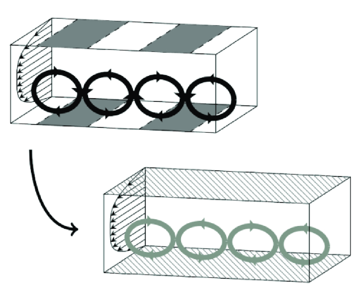
Figure 1. Schematic problem description with a graphical representation of secondary motions. The initial condition (
 $t=0$
) of our numerical set-up is shown in panel (a): steady-state secondary motions are observed over strip-type roughness. A generic point
$t=0$
) of our numerical set-up is shown in panel (a): steady-state secondary motions are observed over strip-type roughness. A generic point
 $t$
in time (with
$t$
in time (with
 $t\gt 0$
) is depicted in panel (b): the secondary motions decay as they evolve over a smooth wall. Box size not to scale. Adapted from Neuhauser et al. (Reference Neuhauser, Schäfer, Gatti and Frohnapfel2022).
$t\gt 0$
) is depicted in panel (b): the secondary motions decay as they evolve over a smooth wall. Box size not to scale. Adapted from Neuhauser et al. (Reference Neuhauser, Schäfer, Gatti and Frohnapfel2022).
We perform direct numerical simulation (DNS) of incompressible channel flows at constant pressure gradient (CPG). The peculiarity of this dataset is that the simulations capture the decay of secondary motions of different sizes; this process is clearly not at a statistically steady state. Rather, our simulations describe the transition from a statistically steady state (flow with secondary motions) to a second steady state (flow in a smooth channel). To still be able to compute averages, each simulation is then run several times, each time starting from a different realisation of a given statistically steady state. Ensemble averages are then calculated.
The channel geometry is shown in figure 1. Let
 $x$
,
$x$
,
 $y$
,
$y$
,
 $z$
be the streamwise, wall-normal and spanwise directions;
$z$
be the streamwise, wall-normal and spanwise directions;
 $u$
,
$u$
,
 $v$
,
$v$
,
 $w$
are the corresponding components of the velocity vector
$w$
are the corresponding components of the velocity vector
 $\boldsymbol {u}$
. The flow is periodic in the streamwise and spanwise directions (periodic boundary conditions); the corresponding periods are indicated as
$\boldsymbol {u}$
. The flow is periodic in the streamwise and spanwise directions (periodic boundary conditions); the corresponding periods are indicated as
 $L_x$
and
$L_x$
and
 $L_z$
, respectively. The flow is statistically homogeneous in the streamwise direction, but not in the spanwise one: indeed, as will be discussed below, a spanwise-heterogeneous (but streamwise-homogeneous) roughness pattern at the wall induces spanwise-heterogeneities of the average flow velocity.
$L_z$
, respectively. The flow is statistically homogeneous in the streamwise direction, but not in the spanwise one: indeed, as will be discussed below, a spanwise-heterogeneous (but streamwise-homogeneous) roughness pattern at the wall induces spanwise-heterogeneities of the average flow velocity.
Time is indicated by
 $t$
. At
$t$
. At
 $t=0$
, the flow is at a statistically steady state in the presence of secondary motions. These are sustained by a spanwise roughness pattern consisting in alternating streamwise-elongated strips of smooth and rough wall. We will refer to this set-up as strip-type roughness. The spanwise width of each strip is
$t=0$
, the flow is at a statistically steady state in the presence of secondary motions. These are sustained by a spanwise roughness pattern consisting in alternating streamwise-elongated strips of smooth and rough wall. We will refer to this set-up as strip-type roughness. The spanwise width of each strip is
 $s$
; the spanwise period of the pattern is
$s$
; the spanwise period of the pattern is
 $\Lambda _s = 2s$
. For
$\Lambda _s = 2s$
. For
 $t\gt 0$
, the spanwise roughness pattern is suddenly replaced by a smooth wall, so that the decay of the secondary motions is observed. The pressure gradient is kept constant in the process.
$t\gt 0$
, the spanwise roughness pattern is suddenly replaced by a smooth wall, so that the decay of the secondary motions is observed. The pressure gradient is kept constant in the process.
Notice, once again, that the flow is streamwise-homogeneous. As the strip-type roughness is removed from the walls, the flow departs from its steady state, but retains its streamwise homogeneity. In other words, the flow develops temporally, but not in the streamwise direction. Our present approach is thus similar to that of Toh & Itano (Reference Toh and Itano2005), in the sense that we investigate the time evolution of streamwise-invariant flow structures. Notice, moreover, that an increase of the bulk velocity is observed as a result of the removal of the strip-type roughness: as the pressure gradient is kept constant, the reduction in skin friction at the wall leads to an increase of the flow rate. Mass is conserved throughout the process: owing to the present geometry, conservation of mass only requires the average flow velocity to be streamwise-invariant, so that time variations of the flow rate are admissible.
Owing to the instationarity and spanwise heterogeneity of the problem, care must be exerted when defining averaging operators and viscous units. The operator
 $ \langle {\cdot } \rangle$
indicates the expected value and is computed as an average over multiple repetitions of the same simulation, over the streamwise direction and over multiple spanwise periods of the selected geometry (phase average, see Reynolds & Hussain Reference Reynolds and Hussain1972); known symmetries in the wall-normal and spanwise directions are used to improve convergence wherever possible. The resulting statistics depend on the conditioned spanwise variable
$ \langle {\cdot } \rangle$
indicates the expected value and is computed as an average over multiple repetitions of the same simulation, over the streamwise direction and over multiple spanwise periods of the selected geometry (phase average, see Reynolds & Hussain Reference Reynolds and Hussain1972); known symmetries in the wall-normal and spanwise directions are used to improve convergence wherever possible. The resulting statistics depend on the conditioned spanwise variable
 $\zeta$
and time, as well as on the wall-normal coordinate
$\zeta$
and time, as well as on the wall-normal coordinate
 $y$
. If an additional spanwise average is performed, the symbol
$y$
. If an additional spanwise average is performed, the symbol
 $ \langle {\cdot } \rangle _z$
is used. As for inner units, the expected value
$ \langle {\cdot } \rangle _z$
is used. As for inner units, the expected value
 $\tau _w(t,\zeta )$
of the wall shear stress is a function of time and of the spanwise coordinate. So are the friction velocity
$\tau _w(t,\zeta )$
of the wall shear stress is a function of time and of the spanwise coordinate. So are the friction velocity
 $u_\tau (t,\zeta ) = \sqrt {\tau _w/\rho }$
and the viscous length scale
$u_\tau (t,\zeta ) = \sqrt {\tau _w/\rho }$
and the viscous length scale
 $\delta _{v}(t,\zeta ) = \nu /u_\tau$
, where
$\delta _{v}(t,\zeta ) = \nu /u_\tau$
, where
 $\rho$
is the density and
$\rho$
is the density and
 $\nu$
the kinematic viscosity. For the calculation of the worst-case inner-scaled grid spacing, the maximum value
$\nu$
the kinematic viscosity. For the calculation of the worst-case inner-scaled grid spacing, the maximum value
 $u_{\tau ,m}$
of the friction velocity can be used:
$u_{\tau ,m}$
of the friction velocity can be used:
 \begin{equation} u_{\tau ,m} = \max _{t,\zeta }\,u_\tau (t,\zeta );\,\,\,\,\,\,\delta _{v,m} = \frac {\nu }{u_{\tau ,m}}. \end{equation}
Leveraging the fact that the pressure gradient
 $-G,\,G\gt 0$
is forcedly kept constant during our simulations, a global friction velocity
$-G,\,G\gt 0$
is forcedly kept constant during our simulations, a global friction velocity
 $u_p$
and length scale
$u_p$
and length scale
 $\delta _{p}$
can also be defined:
$\delta _{p}$
can also be defined:
 \begin{equation} u_p = \sqrt {\frac {hG}{\rho }};\,\,\,\,\,\,\delta _{p} = \frac {\nu }{u_p}. \end{equation}
Quantities scaled with these global viscous units will be indicated with a
 $(\cdot )^+$
superscript. They are also used for the definition of the friction Reynolds number
$(\cdot )^+$
superscript. They are also used for the definition of the friction Reynolds number
 $Re_\tau =hu_p/\nu$
. The relation between global and local viscous units can be found by integrating the streamwise momentum balance of the Navier–Stokes equations. By defining the bulk velocity as the volume-average of the expected streamwise component,
$Re_\tau =hu_p/\nu$
. The relation between global and local viscous units can be found by integrating the streamwise momentum balance of the Navier–Stokes equations. By defining the bulk velocity as the volume-average of the expected streamwise component,
 \begin{equation} U_b(t) = \frac {1}{2h}\int _0^{2h} \left \langle {u} \right \rangle _z \,\text {d}y, \end{equation}
the following relation is obtained:
 \begin{equation} \rho h\frac {\text {d} U_b}{\text {d} t} = hG - \left \langle {\tau _w} \right \rangle _z. \end{equation}
Under steady conditions (
 $t=0$
and
$t=0$
and
 $t\to \infty$
for the problem considered here), the global
$t\to \infty$
for the problem considered here), the global
 $u_p$
is the friction velocity built by using the spanwise average
$u_p$
is the friction velocity built by using the spanwise average
 $ \langle {\tau _w} \rangle _z$
instead of
$ \langle {\tau _w} \rangle _z$
instead of
 $\tau _w$
in its definition:
$\tau _w$
in its definition:
 \begin{align} u_p = \sqrt {\frac {\left \langle {\tau _w} \right \rangle _z}{\rho }}\,\,\,\,\,\,\text {only at a steady state.} \end{align}
2.1. Numerical method and details
We perform DNS using the open-source solver Xcompact3d (Laizet & Lamballais Reference Laizet and Lamballais2009; Laizet & Li Reference Laizet and Li2011; Bartholomew et al. Reference Bartholomew, Deskos, Frantz, Schuch, Lamballais and Laizet2020), using sixth-order compact finite differences in space combined with an explicit third-order Runge–Kutta scheme in time. We test different configurations for varying
 $\Lambda _s$
at two different friction Reynolds numbers (
$\Lambda _s$
at two different friction Reynolds numbers (
 $Re_\tau =180$
and
$Re_\tau =180$
and
 $Re_\tau =500$
). While the streamwise extent
$Re_\tau =500$
). While the streamwise extent
 $L_x$
of the simulation domain is set to values that are greater or equal to those used by Neuhauser et al. (Reference Neuhauser, Schäfer, Gatti and Frohnapfel2022) for analogous simulations, the spanwise box size
$L_x$
of the simulation domain is set to values that are greater or equal to those used by Neuhauser et al. (Reference Neuhauser, Schäfer, Gatti and Frohnapfel2022) for analogous simulations, the spanwise box size
 $L_z$
is set alternatively to
$L_z$
is set alternatively to
 $12h$
,
$12h$
,
 $8h$
or
$8h$
or
 $6h$
to accomodate an integer, even number of strips for each of the tested values of
$6h$
to accomodate an integer, even number of strips for each of the tested values of
 $\Lambda _s$
. The
$\Lambda _s$
. The
 $L_z=6h$
box size is preferred at high-
$L_z=6h$
box size is preferred at high-
 $Re$
wherever possible to minimise the computational load of a single simulation.
$Re$
wherever possible to minimise the computational load of a single simulation.
Our data production pipeline consists of two stages. First, initial conditions are produced by simulating a channel flow with a spanwise roughness pattern of period
 $\Lambda _s$
(see figure 1
a). Rough wall sections are modelled by imposing a slip length
$\Lambda _s$
(see figure 1
a). Rough wall sections are modelled by imposing a slip length
 $\ell$
for the spanwise velocity component at the wall as done by Neuhauser et al. (Reference Neuhauser, Schäfer, Gatti and Frohnapfel2022). This results in the following Robin boundary condition:
$\ell$
for the spanwise velocity component at the wall as done by Neuhauser et al. (Reference Neuhauser, Schäfer, Gatti and Frohnapfel2022). This results in the following Robin boundary condition:
 \begin{equation} w_{w} = \ell \, \hat {n}_{w}\cdot \left ( \nabla w \right )_{w}, \end{equation}
where the
 $(\cdot )_w$
subscript indicates a quantity evaluated at the wall,
$(\cdot )_w$
subscript indicates a quantity evaluated at the wall,
 $\hat {n}_{w}$
a unit vector that is orthogonal to the wall and pointing into the fluid. The value of the slip length is set to
$\hat {n}_{w}$
a unit vector that is orthogonal to the wall and pointing into the fluid. The value of the slip length is set to
 $\ell ^+ = 9$
following Neuhauser et al. (Reference Neuhauser, Schäfer, Gatti and Frohnapfel2022). After the simulation reaches a steady state, a set of
$\ell ^+ = 9$
following Neuhauser et al. (Reference Neuhauser, Schäfer, Gatti and Frohnapfel2022). After the simulation reaches a steady state, a set of
 $N_s$
snapshots is stored; the sample time is set to
$N_s$
snapshots is stored; the sample time is set to
 $1 h/u_p$
to ensure that snapshots are reasonably uncorrelated. As previously explained,
$1 h/u_p$
to ensure that snapshots are reasonably uncorrelated. As previously explained,
 $u_p$
is analogous to
$u_p$
is analogous to
 $u_\tau$
; then, if
$u_\tau$
; then, if
 $h$
is the maximum height of an attached eddy, its lifetime can be expected to be of the order of the eddy turnover time
$h$
is the maximum height of an attached eddy, its lifetime can be expected to be of the order of the eddy turnover time
 $1 h/u_p$
(see, e.g., Lozano-Durán & Jiménez Reference Lozano-Durán and Jiménez2014). One can then expect that the turbulent features observed in a given snapshot differ from those of the successive snapshot saved after
$1 h/u_p$
(see, e.g., Lozano-Durán & Jiménez Reference Lozano-Durán and Jiménez2014). One can then expect that the turbulent features observed in a given snapshot differ from those of the successive snapshot saved after
 $1 h/u_p$
.
$1 h/u_p$
.
Each of the
 $N_s$
saved snapshots of the secondary motions is used as the initial condition for a second simulation between smooth walls (see figure 1
b). The duration of the simulation
$N_s$
saved snapshots of the secondary motions is used as the initial condition for a second simulation between smooth walls (see figure 1
b). The duration of the simulation
 $T_f$
is chosen to satisfactorily capture the decay of the secondary motions. Streamwise-averaged flow fields are stored every
$T_f$
is chosen to satisfactorily capture the decay of the secondary motions. Streamwise-averaged flow fields are stored every
 $0.01 h/u_p$
, even though a laxer time resolution could have been used in retrospect. Streamwise-averaged velocity fields are preferred to three-dimensional snapshots as the present procedure is particularly data intensive. Exploiting the several repetitions of the simulation, a total of
$0.01 h/u_p$
, even though a laxer time resolution could have been used in retrospect. Streamwise-averaged velocity fields are preferred to three-dimensional snapshots as the present procedure is particularly data intensive. Exploiting the several repetitions of the simulation, a total of
 $N_s$
fields at the same time
$N_s$
fields at the same time
 $t$
from the initial conditions are averaged together to produce an ensemble-average of the decaying secondary motions. The whole procedure is repeated for different values of
$t$
from the initial conditions are averaged together to produce an ensemble-average of the decaying secondary motions. The whole procedure is repeated for different values of
 $\Lambda _s$
and
$\Lambda _s$
and
 $Re_\tau$
.
$Re_\tau$
.
Table 1. Numerical details for all tested combinations of
 $\Lambda _s/h$
(the spanwise period of the roughness pattern) and
$\Lambda _s/h$
(the spanwise period of the roughness pattern) and
 $Re_\tau$
for our smooth (steady) and time-evolving simulations. The number of fields used to calculate statistics is indicated by
$Re_\tau$
for our smooth (steady) and time-evolving simulations. The number of fields used to calculate statistics is indicated by
 $N_0=N_s$
(where
$N_0=N_s$
(where
 $N_0$
refers to steady-state simulations,
$N_0$
refers to steady-state simulations,
 $N_s$
to time-evolving ones).
$N_s$
to time-evolving ones).
 $T_f$
indicates the time duration of the decaying simulation,
$T_f$
indicates the time duration of the decaying simulation,
 $L_x$
and
$L_x$
and
 $L_z$
refer to the simulation box size in the streamwise and spanwise directions; the grid spacing is uniform in these two directions and is indicated by
$L_z$
refer to the simulation box size in the streamwise and spanwise directions; the grid spacing is uniform in these two directions and is indicated by
 $\Delta x$
,
$\Delta x$
,
 $\Delta z$
respectively. The wall-normal grid spacings at the wall and centreline are instead indicated by
$\Delta z$
respectively. The wall-normal grid spacings at the wall and centreline are instead indicated by
 $\Delta y_w$
and
$\Delta y_w$
and
 $\Delta y_c$
. The maximum in time, over each grid point and over the three spatial directions (or velocity components) of the Courant–Friedrichs–Lewy (
$\Delta y_c$
. The maximum in time, over each grid point and over the three spatial directions (or velocity components) of the Courant–Friedrichs–Lewy (
 $\text {CFL} = V\Delta t/q$
, where
$\text {CFL} = V\Delta t/q$
, where
 $\Delta t$
is the simulation time step,
$\Delta t$
is the simulation time step,
 $q$
is the grid spacing at some generic point in a given direction and
$q$
is the grid spacing at some generic point in a given direction and
 $V$
is the velocity component at that point in the same direction) and Fourier (
$V$
is the velocity component at that point in the same direction) and Fourier (
 $F\!o = \nu \Delta t / q^2$
) numbers are also reported. The dot to the left of each row indicates the colour used in the following figures to indicate a given value of
$F\!o = \nu \Delta t / q^2$
) numbers are also reported. The dot to the left of each row indicates the colour used in the following figures to indicate a given value of
 $\Lambda _s/h$
.
$\Lambda _s/h$
.

Numerical details for the complete dataset used for this study are reported in table 1. The grid spacing is normalised with the worst-case value
 $\delta _{v,m}$
of the viscous length scale; such a value is usually observed at the initial conditions. Additionally to the decaying simulations, two reference simulations between smooth walls (
$\delta _{v,m}$
of the viscous length scale; such a value is usually observed at the initial conditions. Additionally to the decaying simulations, two reference simulations between smooth walls (
 $Re_\tau =180$
,
$Re_\tau =180$
,
 $Re_\tau =500$
) have been produced using the same grid used for rough simulations. In this case,
$Re_\tau =500$
) have been produced using the same grid used for rough simulations. In this case,
 $N_{0}$
indicates the number of samples used for the calculation of steady-state statistics. Notice that we adjust the number of fields (
$N_{0}$
indicates the number of samples used for the calculation of steady-state statistics. Notice that we adjust the number of fields (
 $N_s$
,
$N_s$
,
 $N_0$
) used for the computation of statistics as we change
$N_0$
) used for the computation of statistics as we change
 $Re_\tau$
and
$Re_\tau$
and
 $\Lambda _s$
; as for the quantification of the degree of statistical convergence, see § 3.5. Generally,
$\Lambda _s$
; as for the quantification of the degree of statistical convergence, see § 3.5. Generally,
 $Re_\tau$
has a favourable effect on the convergence of statistics: as near-wall turbulent structures become smaller with larger
$Re_\tau$
has a favourable effect on the convergence of statistics: as near-wall turbulent structures become smaller with larger
 $Re_\tau$
, a larger number of these features are contained in a single flow snapshot. This yields a quicker falloff of the small-scale noise. It is thus expected that a lower number of snapshots (
$Re_\tau$
, a larger number of these features are contained in a single flow snapshot. This yields a quicker falloff of the small-scale noise. It is thus expected that a lower number of snapshots (
 $N_s$
,
$N_s$
,
 $N_0$
) is required for statistics to converge at high-
$N_0$
) is required for statistics to converge at high-
 $Re_\tau$
. The effect of the period
$Re_\tau$
. The effect of the period
 $\Lambda _s$
depends instead on the size
$\Lambda _s$
depends instead on the size
 $L_z$
of the simulation box. As previously explained, data from the several spanwise periods contained in a single snapshot are averaged together (phase-averaging); the larger the number of periods
$L_z$
of the simulation box. As previously explained, data from the several spanwise periods contained in a single snapshot are averaged together (phase-averaging); the larger the number of periods
 $L_z/\Lambda _s$
in a single snapshot, the lower we expect the required
$L_z/\Lambda _s$
in a single snapshot, the lower we expect the required
 $N_s$
(or
$N_s$
(or
 $N_0$
) to be.
$N_0$
) to be.
3. Theoretical framework
3.1. Triple decomposition; momentum pathways and circulatory motions
Unlike homogeneous flows, which are best described using a Reynolds decomposition, flows featuring secondary motions are commonly described in terms of a triple decomposition. As would be done in a Reynolds decomposition, velocity fluctuations
 $\boldsymbol {u}^{\prime }$
are separated from the expected value
$\boldsymbol {u}^{\prime }$
are separated from the expected value
 $ \langle {\boldsymbol {u}} \rangle$
. Additionally, the expected value
$ \langle {\boldsymbol {u}} \rangle$
. Additionally, the expected value
 $ \langle {\boldsymbol {u}} \rangle$
is further split into its spanwise average
$ \langle {\boldsymbol {u}} \rangle$
is further split into its spanwise average
 $\boldsymbol {U} = \langle {\boldsymbol {u}} \rangle _z$
and a dispersive field
$\boldsymbol {U} = \langle {\boldsymbol {u}} \rangle _z$
and a dispersive field
 $\boldsymbol {u}_d = (\tilde {u},\tilde {v},\tilde {w})$
to yield the triple decomposition. This is done as the expected value
$\boldsymbol {u}_d = (\tilde {u},\tilde {v},\tilde {w})$
to yield the triple decomposition. This is done as the expected value
 $ \langle {\boldsymbol {u}} \rangle$
of the velocity depends on the conditioned spanwise variable
$ \langle {\boldsymbol {u}} \rangle$
of the velocity depends on the conditioned spanwise variable
 $\zeta$
(see § 2); using the triple decomposition, the spanwise-uniform field
$\zeta$
(see § 2); using the triple decomposition, the spanwise-uniform field
 $\boldsymbol {U}$
is separated from the spanwise-heterogeneous dispersive field
$\boldsymbol {U}$
is separated from the spanwise-heterogeneous dispersive field
 $\boldsymbol {u}_d$
,
$\boldsymbol {u}_d$
,
 \begin{equation} \left \langle {\boldsymbol {u}} \right \rangle = \boldsymbol {U} + \boldsymbol {u}_d. \end{equation}
Since only the streamwise component has a non-zero spanwise average for the present geometry,
 \begin{equation} \boldsymbol {U} = U(t,y) \,\hat {x}, \end{equation}
 \begin{equation} \tilde {u} = \left \langle {u} \right \rangle - U(t,y),\,\,\,\,\,\,\tilde {v} = \left \langle {v} \right \rangle ,\,\,\,\,\,\,\tilde {w} = \left \langle {w} \right \rangle , \end{equation}
where
 $\hat {x}$
is a unit vector pointing in the streamwise direction and
$\hat {x}$
is a unit vector pointing in the streamwise direction and
 $U$
will be referred to as the mean velocity profile. The full velocity field then reads
$U$
will be referred to as the mean velocity profile. The full velocity field then reads
 \begin{equation} \boldsymbol {u}(t,x,y,z) \,=\, U(t,y)\,\hat {x} \,+\, \boldsymbol {u}_d(t,y,\zeta (z)) \,+\, \boldsymbol {u}^{\prime}(t,x,y,z). \end{equation}
Note that the averaged fields
 $U$
,
$U$
,
 $\boldsymbol {u}_d$
are streamwise-invariant owing to the channel geometry. This allows to further split the dispersive field
$\boldsymbol {u}_d$
are streamwise-invariant owing to the channel geometry. This allows to further split the dispersive field
 $\boldsymbol {u}_d$
into two separate parts. Indeed, the continuity equation for
$\boldsymbol {u}_d$
into two separate parts. Indeed, the continuity equation for
 $\boldsymbol {u}_d$
reads
$\boldsymbol {u}_d$
reads
 \begin{equation} \frac {\partial \tilde {v}}{\partial y} + \frac {\partial \tilde {w}}{\partial \zeta } = 0 \text {.} \end{equation}
The above equation indicates that the two-dimensional vector field given by
 $\tilde {v}$
and
$\tilde {v}$
and
 $\tilde {w}$
is divergence-less. The distribution of
$\tilde {w}$
is divergence-less. The distribution of
 $\tilde {v}$
can be thus determined if
$\tilde {v}$
can be thus determined if
 $\tilde {w}$
is known (or vice versa), and the two form a single circulatory pattern. Such a cross-sectional circulatory motion is typical of secondary motions (see e.g. Neuhauser et al. Reference Neuhauser, Schäfer, Gatti and Frohnapfel2022) and will be treated separately from the remaining velocity component
$\tilde {w}$
is known (or vice versa), and the two form a single circulatory pattern. Such a cross-sectional circulatory motion is typical of secondary motions (see e.g. Neuhauser et al. Reference Neuhauser, Schäfer, Gatti and Frohnapfel2022) and will be treated separately from the remaining velocity component
 $\tilde {u}$
, which contains the information regarding the momentum pathways (e.g. Womack et al. Reference Womack, Volino, Meneveau and Schultz2022).
$\tilde {u}$
, which contains the information regarding the momentum pathways (e.g. Womack et al. Reference Womack, Volino, Meneveau and Schultz2022).
3.2. Velocity spectra of the dispersive field
In § 4, the dispersive field of the simulated flows will be inspected in real space to reveal the presence of secondary motions and their features. An additional analysis will be performed in spectral space by scrutinising the velocity spectra
 $\Phi _{\tilde {u}\tilde {u}}$
,
$\Phi _{\tilde {u}\tilde {u}}$
,
 $\Phi _{\tilde {v}\tilde {v}}$
,
$\Phi _{\tilde {v}\tilde {v}}$
,
 $\Phi _{\tilde {w}\tilde {w}}$
of the dispersive field. Velocity spectra are typically defined as the Fourier transform of the velocity correlation function (see, e.g., Davidson Reference Davidson2015). Such a definition cannot be used in the present case owing to the periodicity of the dispersive field: a Fourier series is used instead. As an example, the spectrum
$\Phi _{\tilde {w}\tilde {w}}$
of the dispersive field. Velocity spectra are typically defined as the Fourier transform of the velocity correlation function (see, e.g., Davidson Reference Davidson2015). Such a definition cannot be used in the present case owing to the periodicity of the dispersive field: a Fourier series is used instead. As an example, the spectrum
 $\Phi _{\tilde {u}\tilde {u}}$
of
$\Phi _{\tilde {u}\tilde {u}}$
of
 $\tilde {u}$
is defined as
$\tilde {u}$
is defined as
 \begin{equation} \Phi _{\tilde {u}\tilde {u}} = \frac {\mathcal {F}_z\{\tilde {u}\}^\dagger \mathcal {F}_z\{\tilde {u}\}}{\Delta \kappa _z}, \end{equation}
where
 $(\cdot )^\dagger$
indicates the conjugate of a complex number,
$(\cdot )^\dagger$
indicates the conjugate of a complex number,
 $\Delta \kappa _z$
is the Fourier resolution in the spanwise direction and
$\Delta \kappa _z$
is the Fourier resolution in the spanwise direction and
 $\mathcal {F}_z\{\tilde {u}\}$
indicates the coefficients of the Fourier series of
$\mathcal {F}_z\{\tilde {u}\}$
indicates the coefficients of the Fourier series of
 $\tilde {u}$
. These are defined as
$\tilde {u}$
. These are defined as
 \begin{equation} \mathcal {F}_z\{\tilde {u}\} (t,y,\kappa _z) = \frac {1}{\Lambda _s} \int _0^{\Lambda _s} \tilde {u}(t,y,\zeta )\, e^{-i\kappa _z \zeta }\, \text {d}\zeta \end{equation}
where
 $i$
is the imaginary unit and
$i$
is the imaginary unit and
 $\kappa _z$
the spanwise wavenumber. Owing to Parseval’s theorem, the spectrum of
$\kappa _z$
the spanwise wavenumber. Owing to Parseval’s theorem, the spectrum of
 $\tilde {u}$
can be related to the spanwise average of its energy:
$\tilde {u}$
can be related to the spanwise average of its energy:
 \begin{equation} \sum _{\kappa _z=-\infty }^{+\infty } \Delta \kappa _z \Phi _{\tilde {u}\tilde {u}}(t,y,\kappa _z) = \frac {1}{\Lambda _s} \int _{0}^{\Lambda _s} \tilde {u}^2(t,y,\zeta )\,\text {d}\zeta = \big \langle {\tilde {u}^2} \big \rangle _z \end{equation}
The above equation justifies the common interpretation of the spectrum as the contribution of motions of wavelength
 $\lambda _z = 2\pi /\kappa _z$
to the energy of the flow.
$\lambda _z = 2\pi /\kappa _z$
to the energy of the flow.
3.3. Triple-decomposed momentum and velocity budgets
Additionally to the spectra, the energy budget of the streamwise dispersive velocity component
 $\tilde {u}$
will be analysed at a steady state in § 4. For completeness, and to shed light on the way energy is redistributed between the mean, dispersive and fluctuation fields, each of the corresponding budget equations will be presented in the following discussion (including equations that will not be further discussed in the paper). These budget equations can be easily obtained starting from the Reynolds-averaged momentum budget and from the budget equation of the Reynolds stress tensor (see, e.g., Davidson Reference Davidson2015):
$\tilde {u}$
will be analysed at a steady state in § 4. For completeness, and to shed light on the way energy is redistributed between the mean, dispersive and fluctuation fields, each of the corresponding budget equations will be presented in the following discussion (including equations that will not be further discussed in the paper). These budget equations can be easily obtained starting from the Reynolds-averaged momentum budget and from the budget equation of the Reynolds stress tensor (see, e.g., Davidson Reference Davidson2015):
 \begin{align} \frac {\partial \left \langle {u_i} \right \rangle }{\partial t} + \left \langle {u_k} \right \rangle \frac {\partial }{\partial x_k} \left \langle {u_i} \right \rangle & + \frac {1}{\rho }\frac {\partial \left \langle {P} \right \rangle }{\partial x_i} = \nu \nabla ^2 \left \langle {u_i} \right \rangle - \frac {\partial }{\partial x_k}\left \langle {u^{\prime}_i u^{\prime}_k} \right \rangle .\end{align}
 \begin{align} \frac {\partial \big \langle {u^{\prime}_i u^{\prime}_j} \big \rangle }{\partial t} + \left \langle {u_k} \right \rangle \frac {\partial }{\partial x_k} \big \langle {u^{\prime}_i u^{\prime}_j} \big \rangle \,=\, & - \,\left \langle {u^{\prime}_i u^{\prime}_k} \right \rangle \frac {\partial \langle {u_j} \rangle }{\partial x_k} - \big \langle {u^{\prime}_ju^{\prime}_k} \big \rangle \frac {\partial \left \langle {u_i} \right \rangle }{\partial x_k} \nonumber\\ & - \,\frac {\partial }{\partial x_k} \left \langle {u^{\prime}_i u^{\prime}_j u^{\prime}_k} \right \rangle - \frac {\partial }{\partial x_i} \left \langle {u^{\prime}_j\frac {P^{\prime}}{\rho }} \right \rangle - \frac {\partial }{\partial x_j} \left \langle {u^{\prime}_i \frac {P^{\prime}}{\rho }} \right \rangle \nonumber\\ & + \,\left \langle {\frac {P^{\prime}}{\rho }\left (\frac {\partial u^{\prime}_i }{\partial x_j} + \frac {\partial u^{\prime}_j}{\partial x_i}\right )} \right \rangle \nonumber \\ & + \,\nu \nabla ^2 \big \langle {u^{\prime}_i u^{\prime}_j} \big \rangle - 2\nu \left \langle {\frac {\partial u^{\prime}_i }{\partial x_k}\frac {\partial u^{\prime}_j}{\partial x_k}} \right \rangle .\end{align}
The above equations are usually derived by time-averaging, whereas the present work resorts to averaging in the streamwise direction, over multiple repetitions of a simulation and over multiple phases of a periodic domain. Nevertheless, it is trivially shown that the above equations are valid regardless of how averaging is performed as long as the averaging operator fulfils the following properties (as it does in this case):
 \begin{equation} \left \langle {f^\prime } \right \rangle = 0; \,\,\, \left \langle {\left \langle {f} \right \rangle } \right \rangle = \left \langle {f} \right \rangle ; \,\,\, \left \langle {\left \langle {f} \right \rangle f^\prime } \right \rangle = \left \langle {f} \right \rangle \left \langle {f^\prime } \right \rangle ,\end{equation}
where
 $f$
indicates a generic random function. Equation (3.9) is only valid for the expected velocity field
$f$
indicates a generic random function. Equation (3.9) is only valid for the expected velocity field
 $ \langle {\boldsymbol {u}} \rangle$
; leveraging the fact that the triple decomposition is a particular case of the Reynolds one, a budget equation for the
$ \langle {\boldsymbol {u}} \rangle$
; leveraging the fact that the triple decomposition is a particular case of the Reynolds one, a budget equation for the
 $i$
th component
$i$
th component
 $U_i$
of the mean field can be obtained by substituting (3.1) in (3.9) and taking a spanwise average:
$U_i$
of the mean field can be obtained by substituting (3.1) in (3.9) and taking a spanwise average:
 \begin{equation} \frac {\partial U_i}{\partial t} + U_k\frac {\partial U_i}{\partial x_k} + \frac {1}{\rho }\frac {\partial \left \langle {P} \right \rangle _z}{\partial x_i} = \nu \nabla ^2 U_i - \frac {\partial }{\partial x_k}\left \langle {\tilde {u}_i\tilde {u}_k} \right \rangle _z - \frac {\partial }{\partial x_k} \left \langle {u^{\prime}_i u^{\prime}_k} \right \rangle _z. \end{equation}
The above equation resembles the Reynolds-averaged Navier–Stokes momentum equation (3.9), except that an additional term appears. Not only does the mean field feel the presence of turbulence through the Reynolds stress
 $ \langle {u^{\prime}_i u^{\prime}_k} \rangle _z$
, but it is also influenced by the dispersive field through the dispersive stress
$ \langle {u^{\prime}_i u^{\prime}_k} \rangle _z$
, but it is also influenced by the dispersive field through the dispersive stress
 $ \langle {\tilde {u}_i\tilde {u}_k} \rangle _z$
. Notice, moreover, that (2.4), which describes the time-evolution of the bulk velocity, can be obtained by integrating (3.12) over the flow domain. By once again substituting (3.1) in (3.9) and by subtracting (3.12), one obtains a balance equation for the dispersive momentum:
$ \langle {\tilde {u}_i\tilde {u}_k} \rangle _z$
. Notice, moreover, that (2.4), which describes the time-evolution of the bulk velocity, can be obtained by integrating (3.12) over the flow domain. By once again substituting (3.1) in (3.9) and by subtracting (3.12), one obtains a balance equation for the dispersive momentum:
 \begin{align} \frac {\partial \tilde {u}_i}{\partial t} + \left (U_k + \tilde {u}_k\right )\frac {\partial \tilde {u}_i}{\partial x_k} + \frac {1}{\rho }\frac {\partial \tilde {p}}{\partial x_i} = \nu \nabla ^2\tilde {u}_i &\underbrace {- \tilde {u}_k\frac {\partial U_i}{\partial x_k}}_{\text {V4}} + \frac {\partial }{\partial x_k} \left \langle {\tilde {u}_i \tilde {u}_k} \right \rangle _z \\ &- \frac {\partial }{\partial x_k} \left ( \left \langle {u^{\prime}_i u^{\prime}_k} \right \rangle - \left \langle {u^{\prime}_i u^{\prime}_k} \right \rangle _z \right ) \notag, \end{align}
where
 $\tilde {u}_i$
indicates the
$\tilde {u}_i$
indicates the
 $i$
th component of
$i$
th component of
 $\boldsymbol {u}_d$
. Notice that (3.12) and (3.13) are of general validity (symmetries and simplifications due to the geometry have not been considered yet). Starting from the momentum budgets (3.12) and (3.13), energy budgets are trivially obtained by multiplication with
$\boldsymbol {u}_d$
. Notice that (3.12) and (3.13) are of general validity (symmetries and simplifications due to the geometry have not been considered yet). Starting from the momentum budgets (3.12) and (3.13), energy budgets are trivially obtained by multiplication with
 $U_i$
and
$U_i$
and
 $\tilde {u}_i$
, respectively, and by performing a subsequent spanwise average. Additionally, an energy budget for the fluctuation field can be obtained by substituting (3.1) in (3.10) and by spanwise-averaging. After rearranging some terms, one obtains
$\tilde {u}_i$
, respectively, and by performing a subsequent spanwise average. Additionally, an energy budget for the fluctuation field can be obtained by substituting (3.1) in (3.10) and by spanwise-averaging. After rearranging some terms, one obtains
 \begin{align} \frac {\partial }{\partial t}\frac {U_i^2}{2} \,+\, U_k \frac {\partial }{\partial x_k}\frac {U_i^2}{2} \,=\,\, &\nu \nabla ^2\frac {U_i^2}{2} \,-\, \nu \left (\frac {\partial U_i}{\partial x_k}\frac {\partial U_i}{\partial x_k}\right ) \,-\, \frac {U_i}{\rho }\frac {\partial \left \langle {P} \right \rangle _z}{\partial x_i} \\ \notag & + \underbrace {\left \langle {\tilde {u}_i\tilde {u}_k} \right \rangle _z\frac {\partial U_i}{\partial x_k}}_{\text {M5}} \,+\, \left \langle {u^{\prime}_i u^{\prime}_k} \right \rangle _z\frac {\partial U_i}{\partial x_k} \\ \notag &- \frac {\partial }{\partial x_k}\left [ U_i \left ( \left \langle {\tilde {u}_i\tilde {u}_k} \right \rangle _z + \left \langle {u^{\prime}_i u^{\prime}_k} \right \rangle _z \right ) \right ], \end{align}
 \begin{align} \frac {\partial }{\partial t}\frac {\left \langle {\tilde {u}_i^2} \right \rangle _z}{2} \,+\, \underbrace {\frac {\partial }{\partial x_k}\left \langle { (U_k + \tilde {u}_k) \frac {\tilde {u}_i^2}{2} } \right \rangle _z}_{\text {D1}} \,=\,\, &\underbrace {\phantom {\Big |\!}\nu \nabla ^2\frac {\left \langle {\tilde {u}_i^2} \right \rangle _z}{2}}_{\text {D2}} \,\underbrace {-\, \nu \left \langle {\frac {\partial \tilde {u}_i}{\partial x_k}\frac {\partial \tilde {u}_i}{\partial x_k}} \right \rangle _z}_{\text {D3}} \,\underbrace {-\, \left \langle {\frac {\tilde {u}_i}{\rho }\frac {\partial \tilde {P}}{\partial x_i}} \right \rangle _z}_{\text {D4}} \\ \notag & \underbrace {- \left \langle {\tilde {u}_i \tilde {u}_k} \right \rangle _z \frac {\partial U_i}{\partial x_k}}_{\text {D5}} \,+\, \underbrace {\left \langle {\left \langle {u^{\prime}_i u^{\prime}_k} \right \rangle \frac {\partial \tilde {u}_i}{\partial x_k}} \right \rangle _z}_{\text {D6}}\\ \notag & \underbrace {- \frac {\partial }{\partial x_k} \left \langle {\tilde {u}_i\left \langle {u^{\prime}_i u^{\prime}_k} \right \rangle } \right \rangle _z}_{\text {D7}}, \end{align}
 \begin{align} \frac {\partial }{\partial t} \frac {\left \langle {u^{\prime}_i u^{\prime}_i } \right \rangle _z}{2} + \frac {\partial }{\partial x_k}\!\left \langle {\!\left (U_k + \tilde {u}_k\right )\! \frac {\left \langle {u^{\prime}_i u^{\prime}_i } \right \rangle }{2}\!} \right \rangle _z\! =\,\, & + \,\nu \nabla ^2 \frac {\left \langle {u^{\prime}_i u^{\prime}_i } \right \rangle _z}{2} \,-\, \nu \left \langle {\frac {\partial u^{\prime}_i }{\partial x_k}\frac {\partial u^{\prime}_i }{\partial x_k}} \right \rangle _z \notag\\ & - \left \langle {u^{\prime}_i u^{\prime}_k} \right \rangle _z\frac {\partial U_i}{\partial x_k} \,\underbrace {-\, \left \langle {\left \langle {u^{\prime}_i u^{\prime}_k} \right \rangle \frac {\partial \tilde {u}_i}{\partial x_k}} \right \rangle _z}_{\text {F6}} \notag\\ & -\frac {1}{2}\frac {\partial }{\partial x_k} \left \langle {u^{\prime}_i u^{\prime}_i u^{\prime}_k} \right \rangle _z \,-\, \frac {\partial }{\partial x_i} \left \langle {\frac {u^{\prime}_i }{\rho }P^{\prime}} \right \rangle _z. \end{align}
The above equations were also found by Reynolds & Hussain (Reference Reynolds and Hussain1972) using a slightly different averaging technique. Consider the equation for the dispersive kinetic energy (3.15). The dispersive kinetic energy gets transported by both the mean and the dispersive fields (term D1); a pressure term appears in the equation (D4), as well as the usual viscous diffusion (D2) and dissipation (D3) terms. The former indicates that viscosity tends to smear the dispersive energy out over time, whereas the latter represents the power lost to viscous forces. The two remaining equations ((3.14) and (3.16)) all share analogous transport, pressure and viscous terms; the only difference is that the mean kinetic energy
 $U_i^2$
is only transported by the mean field
$U_i^2$
is only transported by the mean field
 $U_i$
, and not by the dispersive one
$U_i$
, and not by the dispersive one
 $\tilde {u}_i$
.
$\tilde {u}_i$
.
Most importantly, the above equations shed a light on how the mean, dispersive and fluctuation fields exchange energy. For instance, the dispersive stress term D5 appears both in the balance of dispersive energy (3.15) and in the balance of mean energy (3.14) (term M5) with opposite sign: it thus represents an exchange of power between the mean and the dispersive fields. Similarly, term D6 represents an exchange of power between the dispersive and fluctuation fields, as it appears both in the dispersive balance and in the fluctuation one (3.16) (term F6) with opposite sign. To sum up, the dispersive stresses enable the exchange of energy between the mean and the dispersive fields, whereas the Reynolds stresses allow the exchange of energy between the dispersive and the fluctuation field (and additionally between the mean and the fluctuation field, as is usual; see (3.14) and (3.16)).
In § 4, only the energy budget of the streamwise dispersive energy
 $\tilde {u}^2$
will be analysed; indeed, the quantities involved in the budgets of the two remaining components
$\tilde {u}^2$
will be analysed; indeed, the quantities involved in the budgets of the two remaining components
 $\tilde {v}^2$
and
$\tilde {v}^2$
and
 $\tilde {w}^2$
are too small compared with the fluctuations to be captured with a satisfactory signal-to-noise ratio. Such a
$\tilde {w}^2$
are too small compared with the fluctuations to be captured with a satisfactory signal-to-noise ratio. Such a
 $\tilde {u}^2$
-budget can be obtained in a similar way to (3.15), but without averaging in the spanwise direction; after considering all the simplifications and symmetries due to the present geometry, the budget reads
$\tilde {u}^2$
-budget can be obtained in a similar way to (3.15), but without averaging in the spanwise direction; after considering all the simplifications and symmetries due to the present geometry, the budget reads
 \begin{align} \frac {\partial }{\partial t} \frac {\tilde {u}^2}{2} + \underbrace {\left ( \tilde {v}\frac {\partial }{\partial y} + \tilde {w}\frac {\partial }{\partial \zeta } \right ) \frac {\tilde {u}^2}{2}}_{\mathcal {T}_a} \,=\, &\underbrace {\nu \nabla ^2\frac {\tilde {u}^2}{2} -\nu \left (\frac {\partial \tilde {u}}{\partial y}\frac {\partial \tilde {u}}{\partial y} + \frac {\partial \tilde {u}}{\partial \zeta }\frac {\partial \tilde {u}}{\partial \zeta } \right )}_{\mathcal {V}} + \underbrace {\tilde {u}\frac {\partial }{\partial y}\left \langle {\tilde {u}\tilde {v}} \right \rangle _z}_{\mathcal {T}_c} \nonumber\\ &\underbrace {-\,\tilde {u}\tilde {v}\frac {\partial U}{\partial y}}_{\mathcal {P}} \underbrace {-\, \tilde {u}\frac {\partial }{\partial y}\left (\left \langle {u^{\prime}v^{\prime}} \right \rangle - \left \langle {u^{\prime}v^{\prime}} \right \rangle _z \right )}_{\mathcal {T}_{uv}} \underbrace {- \tilde {u}\frac {\partial }{\partial \zeta }\left \langle {u^{\prime}w^{\prime}} \right \rangle }_{\mathcal {T}_{uw}}. \end{align}
An additional term appears here with respect to (3.15) – that is,
 $\mathcal {T}_c$
. This term integrates to zero when spanwise-averaged, both explaining its absence from (3.15) and indicating that the term only spatially redistributes
$\mathcal {T}_c$
. This term integrates to zero when spanwise-averaged, both explaining its absence from (3.15) and indicating that the term only spatially redistributes
 $\tilde {u}$
-energy. The remaining terms all have a correspondent in (3.15). Notice that here, both the viscous diffusion (D2 in (3.15)) and the viscous dissipation (D3) are grouped in a single term
$\tilde {u}$
-energy. The remaining terms all have a correspondent in (3.15). Notice that here, both the viscous diffusion (D2 in (3.15)) and the viscous dissipation (D3) are grouped in a single term
 $\mathcal {V}$
. The terms
$\mathcal {V}$
. The terms
 $\mathcal {T}_{uv}$
and
$\mathcal {T}_{uv}$
and
 $\mathcal {T}_{uw}$
quantify the work done by the Reynolds stresses on the dispersive velocity
$\mathcal {T}_{uw}$
quantify the work done by the Reynolds stresses on the dispersive velocity
 $\tilde {u}$
. Such work was rewritten in (3.15) as two separate terms (D6 and D7), of which one (D6) corresponds to a power exchange with the fluctuation field, and the other (D7) can be easily shown to turn zero for the
$\tilde {u}$
. Such work was rewritten in (3.15) as two separate terms (D6 and D7), of which one (D6) corresponds to a power exchange with the fluctuation field, and the other (D7) can be easily shown to turn zero for the
 $\tilde {u}$
component when integrated over the flow domain (notice that the same does not hold for the
$\tilde {u}$
component when integrated over the flow domain (notice that the same does not hold for the
 $w$
component owing to the slip length boundary condition). That is, term D7 only yields a spatial redistribution of
$w$
component owing to the slip length boundary condition). That is, term D7 only yields a spatial redistribution of
 $\tilde {u}$
-energy.
$\tilde {u}$
-energy.
Finally, the
 $\mathcal {P}$
term of (3.17) is of particular interest for the results of this paper. We refer to such a term as dispersive production owing to its similarity to the canonical turbulence production term in a channel flow (Davidson Reference Davidson2015). Such a term corresponds to the D5 term in (3.15), and it thus represents an energy exchange with the mean field. The term accounts for the work done by the momentum flux V4 in (3.13) on the velocity
$\mathcal {P}$
term of (3.17) is of particular interest for the results of this paper. We refer to such a term as dispersive production owing to its similarity to the canonical turbulence production term in a channel flow (Davidson Reference Davidson2015). Such a term corresponds to the D5 term in (3.15), and it thus represents an energy exchange with the mean field. The term accounts for the work done by the momentum flux V4 in (3.13) on the velocity
 $\tilde {u}$
. The momentum flux is better discussed by considering the balance of streamwise momentum and by applying all simplifications due to the geometry:
$\tilde {u}$
. The momentum flux is better discussed by considering the balance of streamwise momentum and by applying all simplifications due to the geometry:
 \begin{equation} -\tilde {v}\frac {\partial U}{\partial y}. \end{equation}
It is clear from (3.18) that the discussed momentum flux originates from
 $\tilde {v}$
transporting the mean field
$\tilde {v}$
transporting the mean field
 $U$
. In other words, the circulatory dispersive
$U$
. In other words, the circulatory dispersive
 $\tilde {v}$
-
$\tilde {v}$
-
 $\tilde {w}$
motions do not directly provide energy to the streamwise component
$\tilde {w}$
motions do not directly provide energy to the streamwise component
 $\tilde {u}$
, but still passively enable the transfer of energy from the mean flow to
$\tilde {u}$
, but still passively enable the transfer of energy from the mean flow to
 $\tilde {u}$
by transporting
$\tilde {u}$
by transporting
 $U$
-momentum. A more intuitive explanation of how the
$U$
-momentum. A more intuitive explanation of how the
 $\tilde {u}$
field is indirectly produced by the circulatory motions (under certain circumstances) will be provided in § 4 using flow visualisations as an example.
$\tilde {u}$
field is indirectly produced by the circulatory motions (under certain circumstances) will be provided in § 4 using flow visualisations as an example.
3.4. Time scale for the decay of secondary motions; volume and plane averages
In § 5, the time needed by secondary motions to decay will be measured as per the objective of this study. Before doing so, such a time scale needs to be defined. Defining a time scale for the decay of turbulent eddies is a largely subjective process. For instance, Flores & Jiménez (Reference Flores and Jiménez2010) found that the log-layer of turbulent flows in a restricted simulation box bursts quasiperiodically, and linked the estimated period to the life span of log-layer eddies. LeHew et al. (Reference LeHew, Guala and McKeon2013) and Lozano-Durán & Jiménez (Reference Lozano-Durán and Jiménez2014), instead, resorted to identifying turbulent coherent structures and tracking them in time; their lifespan is given by the distance in time between their first and last identification. In our case, no sophisticated strategy is needed to track the secondary motions, as their spatial position is fixed and their features are satisfactorily captured by the dispersive velocity field
 $\boldsymbol {u}_d$
(as will be discussed in § 4). We thus define some energy measure
$\boldsymbol {u}_d$
(as will be discussed in § 4). We thus define some energy measure
 $e(t)\geqslant 0$
using the dispersive velocity and track it in time; the energy will start from a value
$e(t)\geqslant 0$
using the dispersive velocity and track it in time; the energy will start from a value
 $e(0)$
seen at the steady state and then decline to zero for
$e(0)$
seen at the steady state and then decline to zero for
 $t\to \infty$
as the secondary motions decay. The time scale
$t\to \infty$
as the secondary motions decay. The time scale
 $T$
for the decay can then be defined as the time required for most of the energy to vanish; more precisely, as the minimum value of
$T$
for the decay can then be defined as the time required for most of the energy to vanish; more precisely, as the minimum value of
 $t$
after which the energy
$t$
after which the energy
 $e$
never exceeds a threshold
$e$
never exceeds a threshold
 $\epsilon$
:
$\epsilon$
:
 \begin{eqnarray} T \,\mid \, e(T)=\epsilon ,\,\, e(T+\Delta t) \lt \epsilon \,\,\,\forall \,\,\, \Delta t \gt 0. \end{eqnarray}
A graphical representation of the above definition is provided in figure 2; in the figure, the generic energy measure
 $e$
is replaced by the volume-averaged quantity
$e$
is replaced by the volume-averaged quantity
 $I_u$
(defined in the next paragraph). The threshold
$I_u$
(defined in the next paragraph). The threshold
 $\epsilon$
is set to
$\epsilon$
is set to
 $15\, \%$
of the initial value
$15\, \%$
of the initial value
 $e(0)$
for multiple reasons. First, having a large threshold is beneficial for the signal-to-noise ratio: the smaller the measured value of
$e(0)$
for multiple reasons. First, having a large threshold is beneficial for the signal-to-noise ratio: the smaller the measured value of
 $e$
, the greater its relative statistical uncertainty. It is moreover desirable to let the value of the threshold depend on the initial condition: secondary motions with different values of
$e$
, the greater its relative statistical uncertainty. It is moreover desirable to let the value of the threshold depend on the initial condition: secondary motions with different values of
 $\Lambda _s/h$
hold different amounts of energy at a steady state (Wangsawijaya & Hutchins Reference Wangsawijaya and Hutchins2022). It would not be sensible, then, to compare the time to decay of secondary motions of different sizes as measured by a fixed
$\Lambda _s/h$
hold different amounts of energy at a steady state (Wangsawijaya & Hutchins Reference Wangsawijaya and Hutchins2022). It would not be sensible, then, to compare the time to decay of secondary motions of different sizes as measured by a fixed
 $\epsilon$
: every secondary motion starts from a different initial energy value. Instead, by letting
$\epsilon$
: every secondary motion starts from a different initial energy value. Instead, by letting
 $\epsilon = 15\, \% \,e(0)$
, the inverse
$\epsilon = 15\, \% \,e(0)$
, the inverse
 $1/T$
of the time scale measures some sort of generalised decay rate (
$1/T$
of the time scale measures some sort of generalised decay rate (
 $1/T$
would exactly be a multiple of the decay rate in the case of an exponential decay).
$1/T$
would exactly be a multiple of the decay rate in the case of an exponential decay).
It remains to be specified which energy measure is used to calculate the time scale. In this respect, two different approaches will be pursued. To begin with, the energy of the dispersive field will be volume-averaged to yield two values
 $I_u$
and
$I_u$
and
 $I_{vw}$
for the streamwise and circulatory patterns, respectively:
$I_{vw}$
for the streamwise and circulatory patterns, respectively:
 \begin{align} I_{u}(t) & = \frac {1}{2h}\int _0^{2h} \frac {1}{2} \big\langle {\tilde {u}^2} \big\rangle _z \,\text {d}y\text {,}\end{align}
 \begin{align} I_{vw}(t) & = \frac {1}{2h}\int _0^{2h} \frac {1}{2} \big\langle {\tilde {v}^2 + \tilde {w}^2} \big\rangle _z \,\text {d}y\text {.} \end{align}
By applying the (3.19) to the above quantities, the time scales
 $T_u$
and
$T_u$
and
 $T_{vw}$
for the streamwise pattern and for the circulatory motions are obtained. The streamwise pattern and the circulatory motions are indeed two separate features of the dispersive fields as discussed in § 3.1; they will be thus treated separately.
$T_{vw}$
for the streamwise pattern and for the circulatory motions are obtained. The streamwise pattern and the circulatory motions are indeed two separate features of the dispersive fields as discussed in § 3.1; they will be thus treated separately.

Figure 2. Graphical representation of the definition of the time
 $T_u$
needed for the pattern of streamwise dispersive velocity to decay. Such a time scale is defined by applying (3.19) to the volume-averaged energy
$T_u$
needed for the pattern of streamwise dispersive velocity to decay. Such a time scale is defined by applying (3.19) to the volume-averaged energy
 $I_u$
. The dark green line represents the time evolution of
$I_u$
. The dark green line represents the time evolution of
 $I_u$
; the lighter green area its
$I_u$
; the lighter green area its
 $95\, \%$
confidence interval (as per § 3.5). Similarly, a marker with an error bar is used to indicate
$95\, \%$
confidence interval (as per § 3.5). Similarly, a marker with an error bar is used to indicate
 $T_u$
and its
$T_u$
and its
 $95\, \%$
confidence interval (see, once again, § 3.5). The horizontal dotted line indicates the threshold value
$95\, \%$
confidence interval (see, once again, § 3.5). The horizontal dotted line indicates the threshold value
 $\epsilon =0.15\, I_u(0)$
used to define
$\epsilon =0.15\, I_u(0)$
used to define
 $T_u$
. Data at
$T_u$
. Data at
 $Re_\tau =500$
,
$Re_\tau =500$
,
 $\Lambda _s/h = 2$
.
$\Lambda _s/h = 2$
.
The above approach defines two scalar quantities –
 $I_u$
and
$I_u$
and
 $I_{vw}$
– which can be easily tracked in time; their interpretation is also straightforward, as they represent the cumulative amount of energy held by secondary motions. However, such an approach is unable to capture the spatial complexity of the secondary motions. To recover some of it, for instance, one might resort to averaging the dispersive energy on wall-parallel planes. As an example, the plane-average
$I_{vw}$
– which can be easily tracked in time; their interpretation is also straightforward, as they represent the cumulative amount of energy held by secondary motions. However, such an approach is unable to capture the spatial complexity of the secondary motions. To recover some of it, for instance, one might resort to averaging the dispersive energy on wall-parallel planes. As an example, the plane-average
 $i_u$
of the streamwise energy is defined as follows:
$i_u$
of the streamwise energy is defined as follows:
 \begin{equation} i_u(t,y) = \frac {1}{2}\big \langle {\tilde {u}^2} \big \rangle _z. \end{equation}
Doing so, wall-normal energy variations can be investigated. Bear in mind (see (3.8)) that the value of
 $i_u$
seen at some wall-normal position
$i_u$
seen at some wall-normal position
 $y$
is equal to the sum of all the energy contributions (as measured by the spectrum
$y$
is equal to the sum of all the energy contributions (as measured by the spectrum
 $\Phi _{\tilde {u}\tilde {u}}$
) of the Fourier modes
$\Phi _{\tilde {u}\tilde {u}}$
) of the Fourier modes
 $\mathcal {F}_z \{\tilde {u}\}$
at that same position
$\mathcal {F}_z \{\tilde {u}\}$
at that same position
 $y$
. Leveraging this property, one can also apply (3.19) of the time scale to the dispersive spectrum
$y$
. Leveraging this property, one can also apply (3.19) of the time scale to the dispersive spectrum
 $\Phi _{\tilde {u}\tilde {u}}$
. The resulting time scale describes the life time of motions of given spanwise wavelength
$\Phi _{\tilde {u}\tilde {u}}$
. The resulting time scale describes the life time of motions of given spanwise wavelength
 $\lambda _z = 2\pi /\kappa _z$
at a given wall-normal height
$\lambda _z = 2\pi /\kappa _z$
at a given wall-normal height
 $y$
.
$y$
.
3.5. Estimation of the dispersive field and uncertainty quantification
As previously explained, expected values are indicated by
 $ \langle {\cdot } \rangle$
throughout the present article. With the exception of this section, the same symbol is also used to indicate the estimates of such expected values as computed using the present data. The estimates deviate from the actual expected values as they are calculated on a sample of finite size; in other words, the estimates are affected by statistical uncertainty. It is assumed that statistical uncertainty dominates other sources of error (such as discretisation and round-off error, or the error introduced by the limited domain size), so that the overall uncertainty on the estimated statistics is given by the statistical uncertainty alone. This section deals with the quantification of such statistical uncertainty.
$ \langle {\cdot } \rangle$
throughout the present article. With the exception of this section, the same symbol is also used to indicate the estimates of such expected values as computed using the present data. The estimates deviate from the actual expected values as they are calculated on a sample of finite size; in other words, the estimates are affected by statistical uncertainty. It is assumed that statistical uncertainty dominates other sources of error (such as discretisation and round-off error, or the error introduced by the limited domain size), so that the overall uncertainty on the estimated statistics is given by the statistical uncertainty alone. This section deals with the quantification of such statistical uncertainty.
In particular, the uncertainty on the dispersive velocity field is of interest – as its values are referenced in the main results of this study. For the sake of clarity, the estimator of the dispersive velocity will be indicated by
 $\breve {u}_i$
, whereas its exact (theoretical) value will be
$\breve {u}_i$
, whereas its exact (theoretical) value will be
 $\tilde {u}_i$
as usual:
$\tilde {u}_i$
as usual:
 \begin{equation} \tilde {u}_i \approx \breve {u}_i. \end{equation}
Here, the subscript
 $i$
indicates the component, so that
$i$
indicates the component, so that
 $(\tilde {u}_1, \tilde {u}_2, \tilde {u}_3) = (\tilde {u}, \tilde {v}, \tilde {w})$
. The dispersive field is estimated through a streamwise-, phase- and ensemble-average; such operation can be reinterpreted as the arithmetic mean of a set of intermediate averages
$(\tilde {u}_1, \tilde {u}_2, \tilde {u}_3) = (\tilde {u}, \tilde {v}, \tilde {w})$
. The dispersive field is estimated through a streamwise-, phase- and ensemble-average; such operation can be reinterpreted as the arithmetic mean of a set of intermediate averages
 $\overline {u}^{x\Delta }_{i,k}$
:
$\overline {u}^{x\Delta }_{i,k}$
:
 \begin{equation} \breve {u}_i = \frac {1}{N_s} \sum _{k=1}^{N_s} \,\underbrace {\frac {\Lambda _s}{L_z}\int _{0}^{L_z} \Delta _z(z+\zeta )\, \left ( \frac {1}{L_x} \int _{0}^{L_x} u_{i,k}-\big \langle {u_{i,k}} \big \rangle _z\, \text {d}x\right )\, \text {d}z}_{\overline {u}^{x\Delta }_{i,k}}, \end{equation}
where the index
 $k$
refers to one of the
$k$
refers to one of the
 $N_s$
repetitions of a given simulation and
$N_s$
repetitions of a given simulation and
 $\Delta _z$
is a Dirac comb function used for the computation of the phase-average; by indicating Dirac’s delta distribution as
$\Delta _z$
is a Dirac comb function used for the computation of the phase-average; by indicating Dirac’s delta distribution as
 $\delta$
,
$\delta$
,
 \begin{equation} \Delta _z = \sum _{j=1}^{L_z/\Lambda _s - 1} \delta \left (z+j\Lambda _s\right ). \end{equation}
The
 $N_s$
values of
$N_s$
values of
 $\overline {u}^{x\Delta }_{i,k}$
computed from the many repetitions of each simulation should be reasonably uncorrelated owing to the discussion of § 2.1. In light of the central limit theorem (Billingsley Reference Billingsley1995), then, the probability distribution function of
$\overline {u}^{x\Delta }_{i,k}$
computed from the many repetitions of each simulation should be reasonably uncorrelated owing to the discussion of § 2.1. In light of the central limit theorem (Billingsley Reference Billingsley1995), then, the probability distribution function of
 $\breve {u}_i$
can be modelled by a normal distribution (indicated by
$\breve {u}_i$
can be modelled by a normal distribution (indicated by
 $\mathcal {N}$
) with mean
$\mathcal {N}$
) with mean
 $\tilde {u}_i$
; its standard deviation
$\tilde {u}_i$
; its standard deviation
 $\breve {\sigma }_i$
can be estimated from the standard deviation
$\breve {\sigma }_i$
can be estimated from the standard deviation
 $\overline {\sigma }^{x\Delta }_i$
of the set of values of
$\overline {\sigma }^{x\Delta }_i$
of the set of values of
 $\overline {u}^{x\Delta }_{i,k}$
(which, in turn, is directly computed):
$\overline {u}^{x\Delta }_{i,k}$
(which, in turn, is directly computed):
 \begin{align} \breve {u}_i & \sim \mathcal {N}\left (\tilde {u}_i, \breve {\sigma }_i\right ), \end{align}
 \begin{align} \breve {\sigma }_i & = \frac {\overline {\sigma }^{x\Delta }_i}{\sqrt {N_s}}.\end{align}
Note that, in the context of the present discussion, the cross-correlation between different components of
 $\breve {u}_i$
is neglected; this simplification does not affect the estimates of the uncertainty on
$\breve {u}_i$
is neglected; this simplification does not affect the estimates of the uncertainty on
 $I_u$
. Owing to the above discussion, the
$I_u$
. Owing to the above discussion, the
 $95\, \%$
confidence interval for the estimate of
$95\, \%$
confidence interval for the estimate of
 $\tilde {u}_i$
is given by
$\tilde {u}_i$
is given by
 \begin{equation} \tilde {u}_i = \breve {u}_i \pm \mathcal {E}\!\left \{\tilde {u}_i\right \} = \breve {u}_i \pm 2\breve {\sigma }_i. \end{equation}
Hence, the uncertainty
 $\mathcal {E}\!\{\tilde {u}_i\}$
can be propagated, as an example, to the energy
$\mathcal {E}\!\{\tilde {u}_i\}$
can be propagated, as an example, to the energy
 $\tilde {u}^2/2$
of the streamwise field:
$\tilde {u}^2/2$
of the streamwise field:
 \begin{equation} \mathcal {E}\!\left \{\frac {\tilde {u}^2}{2}\right \} \,\approx \, \sqrt {\left ( \frac {\text {d} \tilde {u}^2/2}{\text {d} \tilde {u}} \right )_{\breve {u}}^2 \left (\mathcal {E}\!\left \{\tilde {u}\right \}\right )^2 } \,=\, |\breve {u}|\,\mathcal {E}\!\left \{\tilde {u}\right \}. \end{equation}
Next, the uncertainty is propagated to the estimate of
 $I_u$
. In theory, this would require modelling the correlation between the values of
$I_u$
. In theory, this would require modelling the correlation between the values of
 $\tilde {u}^2/2$
at different spatial position. However, a pessimistic estimate of the uncertainty on
$\tilde {u}^2/2$
at different spatial position. However, a pessimistic estimate of the uncertainty on
 $I_u$
can be found as follows. It is assumed that extreme events (meaning events for which
$I_u$
can be found as follows. It is assumed that extreme events (meaning events for which
 $(\overline {u}^{x\Delta })^2/2$
falls outside of the
$(\overline {u}^{x\Delta })^2/2$
falls outside of the
 $95\, \%$
confidence interval for
$95\, \%$
confidence interval for
 $\tilde {u}^2/2$
) happen simultaneously at all spatial positions. In other words, given that an extreme event occurs at some spatial position, one is certain to observe an extreme event at any other spatial position. This is a pessimistic assumption: likely, extreme events are confined in space and do not involve the whole flow domain. However, such an assumption might account for large eddies possibly triggering extended coherent regions of extreme events. In light of the above assumption, the error on
$\tilde {u}^2/2$
) happen simultaneously at all spatial positions. In other words, given that an extreme event occurs at some spatial position, one is certain to observe an extreme event at any other spatial position. This is a pessimistic assumption: likely, extreme events are confined in space and do not involve the whole flow domain. However, such an assumption might account for large eddies possibly triggering extended coherent regions of extreme events. In light of the above assumption, the error on
 $I_u$
is estimated as
$I_u$
is estimated as
 \begin{equation} \mathcal {E}\!\left \{I_u\right \} \,\approx \, \frac {1}{2h} \int _0^{2h} \left \langle {\mathcal {E}\!\left \{\frac {\tilde {u}^2}{2}\right \}} \right \rangle _z \,\text {d}y. \end{equation}
Similar considerations can be leveraged to estimate the uncertainty affecting
 $I_{vw}$
and
$I_{vw}$
and
 $\Phi _{\tilde {u}\tilde {u}}$
.
$\Phi _{\tilde {u}\tilde {u}}$
.
Finally, the uncertainty can be propagated to the time scale
 $T_u$
defined by
$T_u$
defined by
 $I_u$
. To do so, the (estimated) value of the time derivative
$I_u$
. To do so, the (estimated) value of the time derivative
 $I_{u,t}$
of
$I_{u,t}$
of
 $I_u$
at the time
$I_u$
at the time
 $T_u$
is used:
$T_u$
is used:
 \begin{equation} \mathcal {E}\!\left \{T_u\right \} \approx \sqrt {\frac {1}{I_{u,t}^2(T_u)}}\, \mathcal {E}\!\left \{I_u\right \}. \end{equation}
Once again, a similar procedure can be used to quantify the uncertainty on the time scales defined by
 $I_{vw}$
and
$I_{vw}$
and
 $\Phi _{\tilde {u}\tilde {u}}$
.
$\Phi _{\tilde {u}\tilde {u}}$
.
4. Steady-state secondary motions

Figure 3. Inner-scaled premultiplied two-dimensional velocity spectra at
 $y^+=10$
for steady-state simulations. The bar below each panel represents the mode
$y^+=10$
for steady-state simulations. The bar below each panel represents the mode
 $\kappa _x = 0$
, which would otherwise not be visible due to the logarithmic scale. (a) Premultiplied spectrum
$\kappa _x = 0$
, which would otherwise not be visible due to the logarithmic scale. (a) Premultiplied spectrum
 $\kappa _x^+\kappa _z^+\phi _{uu}^+$
of the streamwise fluctuations;
$\kappa _x^+\kappa _z^+\phi _{uu}^+$
of the streamwise fluctuations;
 $Re_\tau =500$
, smooth walls. (b) Premultiplied spectrum of the full streamwise velocity signal (including both the dispersive velocity and fluctuations);
$Re_\tau =500$
, smooth walls. (b) Premultiplied spectrum of the full streamwise velocity signal (including both the dispersive velocity and fluctuations);
 $Re_\tau =500$
,
$Re_\tau =500$
,
 $\Lambda _s/h = 1$
. (c) Premultiplied spectrum
$\Lambda _s/h = 1$
. (c) Premultiplied spectrum
 $\kappa _x^+\kappa _z^+\phi _{uu}^+$
of the streamwise fluctuations;
$\kappa _x^+\kappa _z^+\phi _{uu}^+$
of the streamwise fluctuations;
 $Re_\tau =500$
,
$Re_\tau =500$
,
 $\Lambda _s/h = 1$
(same as panel b, but the contribution of the dispersive velocity is removed).
$\Lambda _s/h = 1$
(same as panel b, but the contribution of the dispersive velocity is removed).
In this section, we analyse the dispersive velocity field (as defined in § 2) at the initial steady state. We argue that the main consequence of the presence of strip-type roughness is the existence of a non-zero dispersive velocity field. Later on, in light of this analysis, the dispersive velocity field will be tracked in time as the secondary motions decay.
The dispersive velocity field is linked to an easily identifiable and isolable feature of the velocity spectra of the investigated flows over heterogeneous roughness. As an example, we compare the two-dimensional streamwise velocity spectra of two flows at
 $Re_\tau =500$
, one of which runs between smooth walls (figure 3
a) whereas the other (figure 3
b) runs over a roughness pattern (
$Re_\tau =500$
, one of which runs between smooth walls (figure 3
a) whereas the other (figure 3
b) runs over a roughness pattern (
 $\Lambda _s/h=1$
). This combination of parameters has been chosen to best highlight the observed behaviour and is representative of the remaining cases. The bar below each panel shows the
$\Lambda _s/h=1$
). This combination of parameters has been chosen to best highlight the observed behaviour and is representative of the remaining cases. The bar below each panel shows the
 $\kappa _x=0$
mode (where
$\kappa _x=0$
mode (where
 $\kappa _x$
is the Fourier wavenumber in the streamwise direction;
$\kappa _x$
is the Fourier wavenumber in the streamwise direction;
 $\kappa _z$
is that in the spanwise direction), which would otherwise not be visible owing to the logarithmic scale. The
$\kappa _z$
is that in the spanwise direction), which would otherwise not be visible owing to the logarithmic scale. The
 $\kappa _x=0$
mode is premultiplied with the Fourier resolution
$\kappa _x=0$
mode is premultiplied with the Fourier resolution
 $\Delta \kappa _x = 2 \pi /L_x$
of the spatial grid. The spectrum is evaluated in proximity of the wall (
$\Delta \kappa _x = 2 \pi /L_x$
of the spatial grid. The spectrum is evaluated in proximity of the wall (
 $y^+=10$
), as, according to the attached eddy model of turbulence (Marusic & Monty Reference Marusic and Monty2019), most scales of motion are observable at this wall-normal location. Further away from the wall, only the largest scales would be visible. This heuristic is confirmed by the spectra of the isolated dispersive motion, later shown in figure 6. Notice that no decomposition is used (unless explicitly stated), so that the spectra include both features linked to velocity fluctuations and to the dispersive velocity.
$y^+=10$
), as, according to the attached eddy model of turbulence (Marusic & Monty Reference Marusic and Monty2019), most scales of motion are observable at this wall-normal location. Further away from the wall, only the largest scales would be visible. This heuristic is confirmed by the spectra of the isolated dispersive motion, later shown in figure 6. Notice that no decomposition is used (unless explicitly stated), so that the spectra include both features linked to velocity fluctuations and to the dispersive velocity.
All panels of figure 3 share the same qualitative spectral peak typical of turbulent fluctuations; in agreement with the attached-eddy hypothesis, most of the energy is seen on
 $(\kappa _x,\kappa _z)$
-modes of roughly constant aspect ratio, meaning that motions that are large in the
$(\kappa _x,\kappa _z)$
-modes of roughly constant aspect ratio, meaning that motions that are large in the
 $x$
-direction also tend to be large in
$x$
-direction also tend to be large in
 $z$
. The dominant feature that differentiates the (a) smooth and the (b) rough spectra is the occurrence of a banded energy pattern at
$z$
. The dominant feature that differentiates the (a) smooth and the (b) rough spectra is the occurrence of a banded energy pattern at
 $\kappa _x=0$
in panel (b). This banded pattern is associated with the dispersive velocity: by removing the latter in panel (c), the energy bands are also eliminated so that the remaning spectrum can be hardly distinguished from that of the smooth case. In other words, the dispersive average captures the main spectral feature differentiating a flow over a smooth wall from that over strip-type roughness.
$\kappa _x=0$
in panel (b). This banded pattern is associated with the dispersive velocity: by removing the latter in panel (c), the energy bands are also eliminated so that the remaning spectrum can be hardly distinguished from that of the smooth case. In other words, the dispersive average captures the main spectral feature differentiating a flow over a smooth wall from that over strip-type roughness.
Nevertheless, further and yet less apparent differences arise between smooth and rough spectra; a separate analysis (not shown for brevity) shows for instance that the spectral peak associated with turbulent fluctuations gets closer to the wall in the presence of a roughness pattern. This is expected: consistently with the protrusion height theory of Luchini et al. (Reference Luchini, Manzo and Pozzi1991), using a sliplength to model roughness (as we do) aims at pulling turbulence fluctuations towards the wall to locally increase the wall shear stress (Gatti et al. Reference Gatti, Stroh, Frohnapfel and Hasegawa2018; Neuhauser et al. Reference Neuhauser, Schäfer, Gatti and Frohnapfel2022). As for the meandering of secondary motions (Wangsawijaya et al. Reference Wangsawijaya, Baidya, Chung, Marusic and Hutchins2020), we do not observe any spectral feature that can be clearly linked to it. Meandering would manifest itself as energy content for
 $\kappa _x\neq 0$
at the same
$\kappa _x\neq 0$
at the same
 $\kappa _z$
values of the banded energy pattern associated with the dispersive velocity. The lack of such features is perhaps a consequence of the relatively low Reynolds number; most importantly, meandering is best observed at larger values of
$\kappa _z$
values of the banded energy pattern associated with the dispersive velocity. The lack of such features is perhaps a consequence of the relatively low Reynolds number; most importantly, meandering is best observed at larger values of
 $y^+$
than that used in figure 3 (Wangsawijaya et al. Reference Wangsawijaya, Baidya, Chung, Marusic and Hutchins2020).
$y^+$
than that used in figure 3 (Wangsawijaya et al. Reference Wangsawijaya, Baidya, Chung, Marusic and Hutchins2020).

Figure 4. Dispersive velocity field at the initial steady state (
 $t=0$
) divided in its streamwise
$t=0$
) divided in its streamwise
 $\tilde {u}^+$
(colour) and circulatory
$\tilde {u}^+$
(colour) and circulatory
 $\tilde {v}^+$
-
$\tilde {v}^+$
-
 $\tilde {w}^+$
(arrows) patterns; all data at
$\tilde {w}^+$
(arrows) patterns; all data at
 $Re_\tau =500$
: (a)
$Re_\tau =500$
: (a)
 $\Lambda _s/h=0.5$
; (b)
$\Lambda _s/h=0.5$
; (b)
 $\Lambda _s/h = 1$
; (c)
$\Lambda _s/h = 1$
; (c)
 $\Lambda _s/h = 2$
; (d)
$\Lambda _s/h = 2$
; (d)
 $\Lambda _s/h = 4$
; (e)
$\Lambda _s/h = 4$
; (e)
 $\Lambda _s/h = 6$
. The arrow length is proportional to the magnitude of the represented vector; the scale is graphically represented above panel (e) and is consistent across all panels. Below each panel, we indicate whether the wall at that spanwise position is rough (black) or smooth (white). A green dot marks the position of the vortex centre as defined later in § 5.1.
$\Lambda _s/h = 6$
. The arrow length is proportional to the magnitude of the represented vector; the scale is graphically represented above panel (e) and is consistent across all panels. Below each panel, we indicate whether the wall at that spanwise position is rough (black) or smooth (white). A green dot marks the position of the vortex centre as defined later in § 5.1.
Having found that the dispersive velocity isolates a distinct feature of the turbulent spectra, we proceed to inspect it both in real and Fourier space. Figure 4 shows the dispersive velocity field for all available values of
 $\Lambda _s/h$
at
$\Lambda _s/h$
at
 $Re_\tau =500$
. The averaged flow fields at
$Re_\tau =500$
. The averaged flow fields at
 $Re_\tau = 180$
(not shown for brevity) return a similar picture. Similarly to other studies concerning secondary motions (Chung et al. Reference Chung, Monty and Hutchins2018) and flow over multi-scale roughness (Barros & Christensen Reference Barros and Christensen2014; Womack et al. Reference Womack, Volino, Meneveau and Schultz2022), these visualisations reveal the presence of high- and low-momentum pathways flanked by circulatory motions. A similar flow topology is also seen in the conditional views of the fluctuation field linked to VLSMs (Hutchins & Marusic Reference Hutchins and Marusic2007b
). For low strip widths (
$Re_\tau = 180$
(not shown for brevity) return a similar picture. Similarly to other studies concerning secondary motions (Chung et al. Reference Chung, Monty and Hutchins2018) and flow over multi-scale roughness (Barros & Christensen Reference Barros and Christensen2014; Womack et al. Reference Womack, Volino, Meneveau and Schultz2022), these visualisations reveal the presence of high- and low-momentum pathways flanked by circulatory motions. A similar flow topology is also seen in the conditional views of the fluctuation field linked to VLSMs (Hutchins & Marusic Reference Hutchins and Marusic2007b
). For low strip widths (
 $\Lambda _s/h \leqslant 2$
roughly), regions of downwash (
$\Lambda _s/h \leqslant 2$
roughly), regions of downwash (
 $\tilde {v}\lt 0$
, or sweep events) coincide with regions of high streamwise momentum, and vice versa for ejection events (
$\tilde {v}\lt 0$
, or sweep events) coincide with regions of high streamwise momentum, and vice versa for ejection events (
 $\tilde {v}\gt 0$
). Secondary motions are confined to a region close to the wall for
$\tilde {v}\gt 0$
). Secondary motions are confined to a region close to the wall for
 $\Lambda _s/h = 0.5$
; they grow taller as the strip width is increased (up to
$\Lambda _s/h = 0.5$
; they grow taller as the strip width is increased (up to
 $\Lambda _s/h \approx 2$
). For
$\Lambda _s/h \approx 2$
). For
 $\Lambda _s/h = 2$
, the secondary motions fill the entire channel half-height; under such conditions, high absolute values of streamwise dispersive momentum (regions of darker colour in figure 4) are seen at two separate wall-normal positions. One is located in the immediate proximity of the wall; here, the spanwise distribution of
$\Lambda _s/h = 2$
, the secondary motions fill the entire channel half-height; under such conditions, high absolute values of streamwise dispersive momentum (regions of darker colour in figure 4) are seen at two separate wall-normal positions. One is located in the immediate proximity of the wall; here, the spanwise distribution of
 $\tilde {u}$
is well described by a square wave. The velocity distribution in this region is a good approximant of the distribution of wall shear stress, which is in turn affected by the square-wave spanwise roughness pattern we impose. Further away from the wall, the
$\tilde {u}$
is well described by a square wave. The velocity distribution in this region is a good approximant of the distribution of wall shear stress, which is in turn affected by the square-wave spanwise roughness pattern we impose. Further away from the wall, the
 $\tilde {u}$
-distribution becomes sinuisoidal in the spanwise direction; a second region of intense momentum appears around
$\tilde {u}$
-distribution becomes sinuisoidal in the spanwise direction; a second region of intense momentum appears around
 $y/h \approx 0.4$
(
$y/h \approx 0.4$
(
 $y^+ \approx 200$
).
$y^+ \approx 200$
).
As the strip width is further increased (roughly
 $\Lambda _s/h \gt 2$
), the circulatory cross-plane motions shown by the
$\Lambda _s/h \gt 2$
), the circulatory cross-plane motions shown by the
 $v$
-
$v$
-
 $w$
vector field are progressively confined to the roughness transitions – that is, the interfaces between adjacent rough and smooth strips. As previously observed for lower strip widths,
$w$
vector field are progressively confined to the roughness transitions – that is, the interfaces between adjacent rough and smooth strips. As previously observed for lower strip widths,
 $\tilde {u}$
and
$\tilde {u}$
and
 $\tilde {v}$
are anti-correlated where these intense circulatory motions are present. At the centre of each strip, instead, the
$\tilde {v}$
are anti-correlated where these intense circulatory motions are present. At the centre of each strip, instead, the
 $\tilde {u}$
-velocity approaches local equilibrium with the wall (Chung et al. Reference Chung, Monty and Hutchins2018; Neuhauser et al. Reference Neuhauser, Schäfer, Gatti and Frohnapfel2022). The expected square-wave pattern of
$\tilde {u}$
-velocity approaches local equilibrium with the wall (Chung et al. Reference Chung, Monty and Hutchins2018; Neuhauser et al. Reference Neuhauser, Schäfer, Gatti and Frohnapfel2022). The expected square-wave pattern of
 $\tilde {u}$
is seen at the wall; moving away from it,
$\tilde {u}$
is seen at the wall; moving away from it,
 $\tilde {u}$
changes in sign at the centre of each strip. For
$\tilde {u}$
changes in sign at the centre of each strip. For
 $\Lambda _s/h = 4$
(figure 4d
), this region of reversed sign is bounded in the wall-normal direction; for
$\Lambda _s/h = 4$
(figure 4d
), this region of reversed sign is bounded in the wall-normal direction; for
 $\Lambda _s/h = 6$
(figure 4
e), instead, it reaches the channel centreline.
$\Lambda _s/h = 6$
(figure 4
e), instead, it reaches the channel centreline.
We explain the observed reversal of the sign of
 $\tilde {u}$
as follows. Consider figure 4(e); the circulatory motions are confined to roughness transitions, whereas the flow above the centre of each strip is distant enough from the roughness transitions (and from the secondary motions) to not feel their effects. Although the wall-normal profile of the
$\tilde {u}$
as follows. Consider figure 4(e); the circulatory motions are confined to roughness transitions, whereas the flow above the centre of each strip is distant enough from the roughness transitions (and from the secondary motions) to not feel their effects. Although the wall-normal profile of the
 $U^+ + \tilde {u}^+$
velocity in the middle of each strip does not match that observed over homogeneous roughness or a homogeneous smooth wall, re-scaling
$U^+ + \tilde {u}^+$
velocity in the middle of each strip does not match that observed over homogeneous roughness or a homogeneous smooth wall, re-scaling
 $U + \tilde {u}$
with the local friction velocity makes it collapse on the homogeneous data (we were able to replicate this result on the present data; see Neuhauser et al. Reference Neuhauser, Schäfer, Gatti and Frohnapfel2022). We say that the
$U + \tilde {u}$
with the local friction velocity makes it collapse on the homogeneous data (we were able to replicate this result on the present data; see Neuhauser et al. Reference Neuhauser, Schäfer, Gatti and Frohnapfel2022). We say that the
 $U + \tilde {u}$
profile at the centre of the strips is at equilibrium with the local surface condition. Similar observations were also put forward by Chung et al. (Reference Chung, Monty and Hutchins2018); notice that the authors show visualisations of the
$U + \tilde {u}$
profile at the centre of the strips is at equilibrium with the local surface condition. Similar observations were also put forward by Chung et al. (Reference Chung, Monty and Hutchins2018); notice that the authors show visualisations of the
 $U+\tilde {u}$
field, whereas figure 4 shows the distribution of
$U+\tilde {u}$
field, whereas figure 4 shows the distribution of
 $\tilde {u}$
alone. Under homogeneous conditions, roughness is typically associated with a drag increase (if the flow rate is kept constant) or a reduction of the flow rate (if the pressure gradient is kept constant) with respect to a flow over an homogeneous smooth wall. If a slip length is used to model the roughness (as is done here), the drag increase at constant flow rate is seen as an increased wall shear stress (in physical terms), which can be exactly calculated as the position of the wall is clearly defined (the same does not hold true for real-life roughness, see e.g. Frohnapfel et al. Reference Frohnapfel, Von Deyn, Yang, Neuhauser, Stroh, Örlü and Gatti2024). Unlike the homogeneous case, the present heterogeneous set-up allows to contemporarily observe both the increase in wall shear stress (in spite of the constant pressure gradient) and the decrease in flow rate. Indeed, the pressure gradient only determines the spanwise-averaged value of the wall shear stress (see (2.4)); locally higher and lower (with respect to the spanwise average) values of the wall shear stress are permitted. Thus, the positive sign of the
$\tilde {u}$
alone. Under homogeneous conditions, roughness is typically associated with a drag increase (if the flow rate is kept constant) or a reduction of the flow rate (if the pressure gradient is kept constant) with respect to a flow over an homogeneous smooth wall. If a slip length is used to model the roughness (as is done here), the drag increase at constant flow rate is seen as an increased wall shear stress (in physical terms), which can be exactly calculated as the position of the wall is clearly defined (the same does not hold true for real-life roughness, see e.g. Frohnapfel et al. Reference Frohnapfel, Von Deyn, Yang, Neuhauser, Stroh, Örlü and Gatti2024). Unlike the homogeneous case, the present heterogeneous set-up allows to contemporarily observe both the increase in wall shear stress (in spite of the constant pressure gradient) and the decrease in flow rate. Indeed, the pressure gradient only determines the spanwise-averaged value of the wall shear stress (see (2.4)); locally higher and lower (with respect to the spanwise average) values of the wall shear stress are permitted. Thus, the positive sign of the
 $\tilde {u}$
-velocity in the thin near-wall region above rough strips reflects a slip-length-induced increase of the wall shear stress; its negative sign further away from the wall (and sufficiently far from the circulatory motions), instead, reflects the reduction of flow rate. By contrast, circulatory motions tend to induce a positive sign of
$\tilde {u}$
-velocity in the thin near-wall region above rough strips reflects a slip-length-induced increase of the wall shear stress; its negative sign further away from the wall (and sufficiently far from the circulatory motions), instead, reflects the reduction of flow rate. By contrast, circulatory motions tend to induce a positive sign of
 $\tilde {u}$
over rough strips. The same line of reasoning can explain the features observed over smooth strips; bear in mind that
$\tilde {u}$
over rough strips. The same line of reasoning can explain the features observed over smooth strips; bear in mind that
 $\tilde {u}$
represents a deviation of the averaged velocity from its spanwise average
$\tilde {u}$
represents a deviation of the averaged velocity from its spanwise average
 $U$
, and not a deviation from some reference homogeneous profile. Notice, finally, that a similar reversal of the sign of the momentum pathways was observed by Medjnoun et al. (Reference Medjnoun, Vanderwel and Ganapathisubramani2020) when studying secondary motions induced by a variation of the wall geometry; in such a case though, the sign reversal is caused by the appearence of dominant tertiary motions and not by the segregation of secondary ones as in this case.
$U$
, and not a deviation from some reference homogeneous profile. Notice, finally, that a similar reversal of the sign of the momentum pathways was observed by Medjnoun et al. (Reference Medjnoun, Vanderwel and Ganapathisubramani2020) when studying secondary motions induced by a variation of the wall geometry; in such a case though, the sign reversal is caused by the appearence of dominant tertiary motions and not by the segregation of secondary ones as in this case.
The sign of
 $\tilde {u}$
in regions where the circulatory motions are strong can be explained by a different mechanism. Both the
$\tilde {u}$
in regions where the circulatory motions are strong can be explained by a different mechanism. Both the
 $\tilde {u}$
-
$\tilde {u}$
-
 $\tilde {v}$
anti-correlation and the fact that large absolute values of the streamwise momentum are seen at a certain distance from the wall in figure 4(c) suggest that the streamwise pattern
$\tilde {v}$
anti-correlation and the fact that large absolute values of the streamwise momentum are seen at a certain distance from the wall in figure 4(c) suggest that the streamwise pattern
 $\tilde {u}$
is mainly generated by transport of the mean velocity field
$\tilde {u}$
is mainly generated by transport of the mean velocity field
 $U$
by wall-normal motions
$U$
by wall-normal motions
 $\tilde {v}$
through the dispersive production mechanism described at the end of § 3.3 (see (3.18)). High-speed fluid from the core of the channel (where the largest values of
$\tilde {v}$
through the dispersive production mechanism described at the end of § 3.3 (see (3.18)). High-speed fluid from the core of the channel (where the largest values of
 $U$
are found) is transported towards the wall by a coherent downwash (
$U$
are found) is transported towards the wall by a coherent downwash (
 $\tilde {v}\lt 0$
) to create coherent high-momentum regions (
$\tilde {v}\lt 0$
) to create coherent high-momentum regions (
 $\tilde {u}\gt 0$
), and vice versa low-speed fluid from the near-wall region is transported upwards to yield low-momentum regions. The wall-normal component
$\tilde {u}\gt 0$
), and vice versa low-speed fluid from the near-wall region is transported upwards to yield low-momentum regions. The wall-normal component
 $\tilde {v}$
is expected to be small in proximity of the wall, both due to the impermeability condition and to the topology of the
$\tilde {v}$
is expected to be small in proximity of the wall, both due to the impermeability condition and to the topology of the
 $\tilde {v}$
-
$\tilde {v}$
-
 $\tilde {w}$
circulatory motion. Consequently, we expect
$\tilde {w}$
circulatory motion. Consequently, we expect
 $\tilde {v}$
to be most effective at leveraging
$\tilde {v}$
to be most effective at leveraging
 $\tilde {u}$
-production at a given distance from the wall, as we observe.
$\tilde {u}$
-production at a given distance from the wall, as we observe.

Figure 5. Inner-scaled premultiplied terms of the budget equation for the dispersive
 $\tilde {u}^2/2$
energy (3.17). All data at
$\tilde {u}^2/2$
energy (3.17). All data at
 $Re_\tau =500$
, steady state. Panels (a–d) show data for
$Re_\tau =500$
, steady state. Panels (a–d) show data for
 $\Lambda _s/h=2$
; (a) premultiplied dispersive production
$\Lambda _s/h=2$
; (a) premultiplied dispersive production
 $y^+\mathcal {P}^+$
, (b) viscous term
$y^+\mathcal {P}^+$
, (b) viscous term
 $y^+\mathcal {V}^+$
, (c) contribution
$y^+\mathcal {V}^+$
, (c) contribution
 $y^+\mathcal {T}_{uv}^+$
of the
$y^+\mathcal {T}_{uv}^+$
of the
 $\,\langle {u^{\prime}v^{\prime}} \rangle \,$
Reynolds stress and (d) contribution
$\,\langle {u^{\prime}v^{\prime}} \rangle \,$
Reynolds stress and (d) contribution
 $y^+\mathcal {T}_{uw}^+$
of the
$y^+\mathcal {T}_{uw}^+$
of the
 $\,\langle {u^{\prime}w^{\prime}} \rangle \,$
stress. Panels (e–h): same as panels (a–d) but for
$\,\langle {u^{\prime}w^{\prime}} \rangle \,$
stress. Panels (e–h): same as panels (a–d) but for
 $\Lambda _s/h=6$
. The vertical, dotted lines in panels (e–h) roughly mark the boundary between the equilibrium and the anti-correlation regions. Please note the different scale of the horizontal axis.
$\Lambda _s/h=6$
. The vertical, dotted lines in panels (e–h) roughly mark the boundary between the equilibrium and the anti-correlation regions. Please note the different scale of the horizontal axis.
To corroborate the above idea, we compute the terms of the
 $\tilde {u}^2$
-energy budget (3.17). Such terms are shown in figure 5 at the initial steady state for two selected flow cases (
$\tilde {u}^2$
-energy budget (3.17). Such terms are shown in figure 5 at the initial steady state for two selected flow cases (
 $Re_\tau =500$
,
$Re_\tau =500$
,
 $\Lambda _s/h = 2$
and
$\Lambda _s/h = 2$
and
 $\Lambda _s/h=6$
). The advection terms
$\Lambda _s/h=6$
). The advection terms
 $\mathcal {T}_a$
and
$\mathcal {T}_a$
and
 $\mathcal {T}_c$
are not shown: although their absolute values are not exactly negligible, they are small enough to be dominated by the remaining source (or sink) terms. Positive values of each term indicate that the term is providing energy to the
$\mathcal {T}_c$
are not shown: although their absolute values are not exactly negligible, they are small enough to be dominated by the remaining source (or sink) terms. Positive values of each term indicate that the term is providing energy to the
 $\tilde {u}$
pattern, or, in other words, that the term acts to sustain the dispersive velocity. Negative values, instead, indicate that energy is being subtracted. As previously stated, while
$\tilde {u}$
pattern, or, in other words, that the term acts to sustain the dispersive velocity. Negative values, instead, indicate that energy is being subtracted. As previously stated, while
 $\tilde {u}$
and
$\tilde {u}$
and
 $\tilde {v}$
are everywhere anti-correlated for
$\tilde {v}$
are everywhere anti-correlated for
 $\Lambda _s/h = 2$
, the anti-correlation region is restricted to
$\Lambda _s/h = 2$
, the anti-correlation region is restricted to
 $2h$
-wide neighbourhoods of each roughness transition for
$2h$
-wide neighbourhoods of each roughness transition for
 $\Lambda _s/h = 6$
. We mark the borders of this region with dotted lines in panels (e–h); we refer to the remaining portion of the channel as the equilibrium region. There, the wall-normal profile of
$\Lambda _s/h = 6$
. We mark the borders of this region with dotted lines in panels (e–h); we refer to the remaining portion of the channel as the equilibrium region. There, the wall-normal profile of
 $U+\tilde {u}$
is indeed roughly at equilibrium with the local wall shear stress (see the discussion above).
$U+\tilde {u}$
is indeed roughly at equilibrium with the local wall shear stress (see the discussion above).
The main outer-layer (
 $y^+ \gt 10$
) energy donor in the anti-correlation regions of both considered flow cases is the dispersive production term (figure 5
a,e); all remaining terms are negative, except for a minor positive contribution from
$y^+ \gt 10$
) energy donor in the anti-correlation regions of both considered flow cases is the dispersive production term (figure 5
a,e); all remaining terms are negative, except for a minor positive contribution from
 $ \langle {u^{\prime}v^{\prime}} \rangle$
in panel (c) towards the centreline. The dispersive production term is maximum around
$ \langle {u^{\prime}v^{\prime}} \rangle$
in panel (c) towards the centreline. The dispersive production term is maximum around
 $y^+\approx 200$
; in this same region, intense values of
$y^+\approx 200$
; in this same region, intense values of
 $\tilde {u}$
were found in figure 4(c). This is further evidence in favour of our hypothesis that
$\tilde {u}$
were found in figure 4(c). This is further evidence in favour of our hypothesis that
 $\tilde {v}$
-transport of
$\tilde {v}$
-transport of
 $U$
drives the formation of the
$U$
drives the formation of the
 $\tilde {u}$
pattern. It is also reminiscent of linear-transient growth analysis: the energy growth of optimally amplified modes found by studying the evolution of perturbations in linearised channel flows is driven by the same mechanism (Del Álamo & Jiménez Reference Del Álamo and Jiménez2006).
$\tilde {u}$
pattern. It is also reminiscent of linear-transient growth analysis: the energy growth of optimally amplified modes found by studying the evolution of perturbations in linearised channel flows is driven by the same mechanism (Del Álamo & Jiménez Reference Del Álamo and Jiménez2006).
Both for the narrower and wider strips, the energy budget is dominated by the viscous (figure 5
b,f) and
 $ \langle {u^{\prime}v^{\prime}} \rangle$
(figure 5
c,g) terms in the near-wall region (
$ \langle {u^{\prime}v^{\prime}} \rangle$
(figure 5
c,g) terms in the near-wall region (
 $y^+ \lt 10$
). The former extracts energy from the intense near-wall
$y^+ \lt 10$
). The former extracts energy from the intense near-wall
 $\tilde {u}$
pattern; most of this energy is dissipated, while part of it is returned to the flow just above
$\tilde {u}$
pattern; most of this energy is dissipated, while part of it is returned to the flow just above
 $y^+=10$
, where the term has a weak positive value (this is better observable in panel f). The
$y^+=10$
, where the term has a weak positive value (this is better observable in panel f). The
 $ \langle {u^{\prime}v^{\prime}} \rangle$
stress, instead, is the main provider of energy in this region. This suggests that the formation of the near-wall
$ \langle {u^{\prime}v^{\prime}} \rangle$
stress, instead, is the main provider of energy in this region. This suggests that the formation of the near-wall
 $\tilde {u}$
pattern might be driven by turbulence through the Reynolds shear stress; such an interpretation is coherent with our previous findings (Andreolli et al. Reference Andreolli, Gatti, Vinuesa, Örlü and Schlatter2023), that blocking the energy exchange between small turbulent fluctuations and large ones prevents the formation of large-scaled patterns of wall shear stress. Interestingly, the
$\tilde {u}$
pattern might be driven by turbulence through the Reynolds shear stress; such an interpretation is coherent with our previous findings (Andreolli et al. Reference Andreolli, Gatti, Vinuesa, Örlü and Schlatter2023), that blocking the energy exchange between small turbulent fluctuations and large ones prevents the formation of large-scaled patterns of wall shear stress. Interestingly, the
 $ \langle {u^{\prime}v^{\prime}} \rangle$
term is also the main source of energy in the equilibrium region for the higher strip width (panel g), indicating that it might be responsible for driving the flow towards equilibrium. This is reasonable, as under homogeneous conditions, the mean velocity profile results from the equilibrium of viscous and
$ \langle {u^{\prime}v^{\prime}} \rangle$
term is also the main source of energy in the equilibrium region for the higher strip width (panel g), indicating that it might be responsible for driving the flow towards equilibrium. This is reasonable, as under homogeneous conditions, the mean velocity profile results from the equilibrium of viscous and
 $ \langle {u^{\prime}v^{\prime}} \rangle$
stresses only. However, in the present context, the
$ \langle {u^{\prime}v^{\prime}} \rangle$
stresses only. However, in the present context, the
 $ \langle {u^{\prime}w^{\prime}} \rangle$
term also provides a non-negligible (negative) contribution in the equilibrium region.
$ \langle {u^{\prime}w^{\prime}} \rangle$
term also provides a non-negligible (negative) contribution in the equilibrium region.

Figure 6. Premultiplied one-dimensional energy spectra of the streamwise (a,d;
 $\kappa _z^+\Phi _{\tilde {u}\tilde {u}}^+$
), wall-normal (b,e;
$\kappa _z^+\Phi _{\tilde {u}\tilde {u}}^+$
), wall-normal (b,e;
 $\kappa _z^+\Phi _{\tilde {v}\tilde {v}}^+$
) and spanwise (c,f;
$\kappa _z^+\Phi _{\tilde {v}\tilde {v}}^+$
) and spanwise (c,f;
 $\kappa _z^+\Phi _{\tilde {w}\tilde {w}}^+$
) dispersive velocity components. All data at
$\kappa _z^+\Phi _{\tilde {w}\tilde {w}}^+$
) dispersive velocity components. All data at
 $Re_\tau =500$
. (a,b,c)
$Re_\tau =500$
. (a,b,c)
 $\Lambda _s/h = 2$
; (d,e,f)
$\Lambda _s/h = 2$
; (d,e,f)
 $\Lambda _s/h = 6$
. Below each panel, we show the spanwise power spectral density of the square-wave signal indicating whether the wall is rough (signal
$\Lambda _s/h = 6$
. Below each panel, we show the spanwise power spectral density of the square-wave signal indicating whether the wall is rough (signal
 $=1$
) or smooth (signal
$=1$
) or smooth (signal
 $= 0$
); such a power spectral density is zero almost everywhere. The harmonic number
$= 0$
); such a power spectral density is zero almost everywhere. The harmonic number
 $\Lambda _s/\lambda _z$
associated with each Fourier mode is shown at the top of each panel. Selected local extrema of each spectrum are marked as
$\Lambda _s/\lambda _z$
associated with each Fourier mode is shown at the top of each panel. Selected local extrema of each spectrum are marked as
 $\times$
(white, maxima) and
$\times$
(white, maxima) and
 $+$
(black, minima).
$+$
(black, minima).
Next, we inspect the dispersive velocity field in spectral space. Its spanwise spectra (defined in § 3.2) at the initial steady state are shown in figure 6 for
 $\Lambda _s/h =2,\,6$
and
$\Lambda _s/h =2,\,6$
and
 $Re_\tau =500$
. Notice that, much like the dispersive velocity, these steady-state spectra only depend on the wall-normal coordinate
$Re_\tau =500$
. Notice that, much like the dispersive velocity, these steady-state spectra only depend on the wall-normal coordinate
 $y$
and the spanwise wavenumber
$y$
and the spanwise wavenumber
 $\kappa _z$
. The spectra better show the striped structure that was observed in figure 3; a similar pattern has also been found experimentally by Wangsawijaya & Hutchins (Reference Wangsawijaya and Hutchins2022). We suggest that the striped appearance is caused by the square-wave shape of the roughness pattern we apply at the wall, whose power spectral density (shown below each panel) is also striped. It is indeed observed that most of the energy of the dispersive velocity field is found on the same Fourier modes that are excited by the roughness pattern. For both the roughness pattern and the velocity field, the first harmonic of the Fourier transform usually holds the most energy. The first harmonic is the Fourier mode whose spanwise wavelength
$\kappa _z$
. The spectra better show the striped structure that was observed in figure 3; a similar pattern has also been found experimentally by Wangsawijaya & Hutchins (Reference Wangsawijaya and Hutchins2022). We suggest that the striped appearance is caused by the square-wave shape of the roughness pattern we apply at the wall, whose power spectral density (shown below each panel) is also striped. It is indeed observed that most of the energy of the dispersive velocity field is found on the same Fourier modes that are excited by the roughness pattern. For both the roughness pattern and the velocity field, the first harmonic of the Fourier transform usually holds the most energy. The first harmonic is the Fourier mode whose spanwise wavelength
 $\lambda _z$
matches the period
$\lambda _z$
matches the period
 $\Lambda _s$
of the original signal; higher harmonics have a wavelength that is a fraction of such a period. For convenience, we define a harmonic number
$\Lambda _s$
of the original signal; higher harmonics have a wavelength that is a fraction of such a period. For convenience, we define a harmonic number
 $\Lambda _s/\lambda _z$
, such that the first harmonic has
$\Lambda _s/\lambda _z$
, such that the first harmonic has
 $\Lambda _s/\lambda _z = 1$
, the second
$\Lambda _s/\lambda _z = 1$
, the second
 $\Lambda _s/\lambda _z = 2$
and so on. The harmonic number is shown at the top of each panel in figure 6.
$\Lambda _s/\lambda _z = 2$
and so on. The harmonic number is shown at the top of each panel in figure 6.
In proximity of the wall, energy is seen on a wide range of wavelengths, reinforcing the idea that the velocity distribution there roughly takes the shape of a square wave. As a rule of thumb, energy is restricted to progressively larger Fourier modes as one moves away from the wall, this being reminiscent of the attached eddy hypothesis (see, for instance, Baars et al. Reference Baars, Hutchins and Marusic2017), until the velocity field is dominated by a single sinusoidal wave at the centreline. There is however a notable exception to this trend of larger Fourier modes being taller in the wall-normal direction. This is seen for
 $\Lambda _s/h = 6$
(panel d): the amount of energy on the first harmonic at the centreline is unexpectedly negligible, whereas most of the energy is found on the third harmonic. Similarly, the third harmonic of the
$\Lambda _s/h = 6$
(panel d): the amount of energy on the first harmonic at the centreline is unexpectedly negligible, whereas most of the energy is found on the third harmonic. Similarly, the third harmonic of the
 $\tilde {v}$
distribution (panel e) has the largest energy values throughout the channel height. This behaviour can also be observed without premultiplication of the spectrum; it is not as pronounced at the lower Reynolds number (
$\tilde {v}$
distribution (panel e) has the largest energy values throughout the channel height. This behaviour can also be observed without premultiplication of the spectrum; it is not as pronounced at the lower Reynolds number (
 $Re_\tau = 180$
).
$Re_\tau = 180$
).
Although the roughness pattern significantly excites the first harmonic, it fails to leverage a secondary motion of matching size if its period is too large (
 $\Lambda _s/h = 6$
); rather, the response of the flow contains a substantial amount of energy on a narrower – but still
$\Lambda _s/h = 6$
); rather, the response of the flow contains a substantial amount of energy on a narrower – but still
 $h$
-scaled – wavelength. The wavelength of the dominant harmonic (
$h$
-scaled – wavelength. The wavelength of the dominant harmonic (
 $\lambda _z = 2h$
) of panels (d,e) suggests this might be linked to the observed confinement of secondary motions to a
$\lambda _z = 2h$
) of panels (d,e) suggests this might be linked to the observed confinement of secondary motions to a
 $2h$
-wide region about the spanwise surface transitions (see figure 4
e). As confirmed by a separate analysis of artificial signals, this is likely true for the pattern of
$2h$
-wide region about the spanwise surface transitions (see figure 4
e). As confirmed by a separate analysis of artificial signals, this is likely true for the pattern of
 $\tilde {v}$
. The
$\tilde {v}$
. The
 $\tilde {u}$
-spectrum must be interpreted with care instead: the dominance of the
$\tilde {u}$
-spectrum must be interpreted with care instead: the dominance of the
 $\lambda _z = 2h$
mode might be an artefact caused by the specific value (
$\lambda _z = 2h$
mode might be an artefact caused by the specific value (
 $\Lambda _s=6h$
) of the period of the roughness pattern. Roughness transitions are flanked by a high- and a low-momentum pathway, each of which has a
$\Lambda _s=6h$
) of the period of the roughness pattern. Roughness transitions are flanked by a high- and a low-momentum pathway, each of which has a
 $1h$
width. The remaining space between adjacent roughness transitions is then occupied by a local-equilibrium region where
$1h$
width. The remaining space between adjacent roughness transitions is then occupied by a local-equilibrium region where
 $\tilde {u}$
has opposite sign with respect to the secondary-motion-induced momentum pathways that surround it. This equilibrium region has a width of
$\tilde {u}$
has opposite sign with respect to the secondary-motion-induced momentum pathways that surround it. This equilibrium region has a width of
 $3h - 2h = 1h$
, so that effectively the spanwise
$3h - 2h = 1h$
, so that effectively the spanwise
 $\tilde {u}$
distribution at the centreline is well described by a sinusoid of period
$\tilde {u}$
distribution at the centreline is well described by a sinusoid of period
 $2h$
. This is captured by the Fourier transform, whose dominant mode is not the first harmonic, but rather that with a
$2h$
. This is captured by the Fourier transform, whose dominant mode is not the first harmonic, but rather that with a
 $2h$
wavelength. If the strip width were larger, the width of the anti-correlation region would likely remain constant, whereas the equilibrium region would get larger. In this case, the first harmonic might be dominant even at the centreline (depending on the relative intensity between the values of
$2h$
wavelength. If the strip width were larger, the width of the anti-correlation region would likely remain constant, whereas the equilibrium region would get larger. In this case, the first harmonic might be dominant even at the centreline (depending on the relative intensity between the values of
 $\tilde {u}$
in the equilibrium and anti-correlation regions).
$\tilde {u}$
in the equilibrium and anti-correlation regions).
Several wall-normal gaps, or minima, can be observed in the vertical stripes of the spectra. Most
 $w$
-modes contain one such gap: as an example, in figure 6(f), at
$w$
-modes contain one such gap: as an example, in figure 6(f), at
 $y/h=0.4103$
(first harmonic, see the mark in figure) and
$y/h=0.4103$
(first harmonic, see the mark in figure) and
 $y/h=0.3181$
(third harmonic). Analogous minima of the spectrum can be observed for the remaining energy-containing modes (as well as in panel c) by adjusting the colour scale. We interpret these minima to be the centres of rotation of the circulatory motions associated with each of these Fourier modes. Indeed,
$y/h=0.3181$
(third harmonic). Analogous minima of the spectrum can be observed for the remaining energy-containing modes (as well as in panel c) by adjusting the colour scale. We interpret these minima to be the centres of rotation of the circulatory motions associated with each of these Fourier modes. Indeed,
 $w$
-energy is expected at the bottom and top of these wall-attached circulatory motions as previously shown. Also, coherently with our previous observations,
$w$
-energy is expected at the bottom and top of these wall-attached circulatory motions as previously shown. Also, coherently with our previous observations,
 $\tilde {v}$
energy is not seen at the wall; rather, its global maximum is seen between
$\tilde {v}$
energy is not seen at the wall; rather, its global maximum is seen between
 $y/h \approx 0.3$
and
$y/h \approx 0.3$
and
 $y/h \approx 0.4$
(
$y/h \approx 0.4$
(
 $y^+ \approx 150{-}200$
) both for
$y^+ \approx 150{-}200$
) both for
 $\Lambda _s/h = 2$
and
$\Lambda _s/h = 2$
and
 $\Lambda _s/h = 6$
(first harmonic in panel b and third one in panel e, respectively; see the marks in the figure). A local maximum of
$\Lambda _s/h = 6$
(first harmonic in panel b and third one in panel e, respectively; see the marks in the figure). A local maximum of
 $\tilde {u}$
-energy is seen on matching harmonics at matching wall-normal positions, consistently with the idea that the
$\tilde {u}$
-energy is seen on matching harmonics at matching wall-normal positions, consistently with the idea that the
 $\tilde {u}$
pattern is generated by
$\tilde {u}$
pattern is generated by
 $\tilde {v}$
transporting the mean velocity profile
$\tilde {v}$
transporting the mean velocity profile
 $U$
. Finally, we suggest that the short energy gap seen at the wall on the first
$U$
. Finally, we suggest that the short energy gap seen at the wall on the first
 $\tilde {u}$
-harmonic for the
$\tilde {u}$
-harmonic for the
 $\Lambda _s/h = 6$
case is linked to the change in sign seen in physical space at a matching wall-normal distance at the centre of each strip.
$\Lambda _s/h = 6$
case is linked to the change in sign seen in physical space at a matching wall-normal distance at the centre of each strip.
5. Decaying secondary motions

Figure 7. Time evolution (a) of the bulk velocity (solid,
 $U_b/U_b(0)$
) normalised by its initial, steady-state value and of the inner-scaled spanwise-averaged wall shear stress (dashed,
$U_b/U_b(0)$
) normalised by its initial, steady-state value and of the inner-scaled spanwise-averaged wall shear stress (dashed,
 $\langle {\tau _w} \rangle _z^+$
);
$\langle {\tau _w} \rangle _z^+$
);
 $Re_\tau =500$
,
$Re_\tau =500$
,
 $\Lambda _s/h=2$
(green, as of table 1) and
$\Lambda _s/h=2$
(green, as of table 1) and
 $\Lambda _s/h=6$
(red). Decaying dispersive velocity field:
$\Lambda _s/h=6$
(red). Decaying dispersive velocity field:
 $Re_\tau =500$
,
$Re_\tau =500$
,
 $\Lambda _s/h = 2$
, (b)
$\Lambda _s/h = 2$
, (b)
 $t=1h/u_p$
and (c)
$t=1h/u_p$
and (c)
 $t=3.2h/u_p$
. Panels (d,e): same as panels (b,c), but for
$t=3.2h/u_p$
. Panels (d,e): same as panels (b,c), but for
 $\Lambda _s/h=6$
. Colour and arrow lengths as in figure 4. Below each panel, a grey fill indicates portions of the wall that were rough at the initial condition.
$\Lambda _s/h=6$
. Colour and arrow lengths as in figure 4. Below each panel, a grey fill indicates portions of the wall that were rough at the initial condition.
We now turn our attention to the time evolution of the secondary motions. As explained in § 2, their decay is triggered by suddenly removing the roughness strips from the walls. The process happens at a constant pressure gradient; the sudden removal of the roughness allows the flow rate to increase, as shown in figure 7(a) for two combinations of
 $\Lambda _s$
and
$\Lambda _s$
and
 $Re_\tau$
chosen as an example. Coherently with (2.4), the increase in bulk velocity is driven by a temporary drop of the wall shear stress. As the flow approaches a new steady state for
$Re_\tau$
chosen as an example. Coherently with (2.4), the increase in bulk velocity is driven by a temporary drop of the wall shear stress. As the flow approaches a new steady state for
 $t\to \infty$
, the inner-scaled wall shear stress recovers its typical unitary value; however, this final equilibrium is reached at a point in time that exceeds the duration of our simulations, which only capture the decay of the dispersive velocity field. In other words, the spanwise-averaged field
$t\to \infty$
, the inner-scaled wall shear stress recovers its typical unitary value; however, this final equilibrium is reached at a point in time that exceeds the duration of our simulations, which only capture the decay of the dispersive velocity field. In other words, the spanwise-averaged field
 $U$
evolves at a different rate from that of secondary motions.
$U$
evolves at a different rate from that of secondary motions.
Videos of the decaying dispersive velocity field are available (see Supplementary data at the end of § 7); as an example, snapshots at two different instants of time are shown in figure 7 for
 $Re_\tau =500$
, (b,c)
$Re_\tau =500$
, (b,c)
 $\Lambda _s/h = 2$
and (d,e)
$\Lambda _s/h = 2$
and (d,e)
 $\Lambda _s/h = 6$
. The typical qualitative picture of the decay for low values of
$\Lambda _s/h = 6$
. The typical qualitative picture of the decay for low values of
 $\Lambda _s/h$
, which is well represented by panels (b,c), is rather straightforward. The secondary motions slowly fade away, while the intense
$\Lambda _s/h$
, which is well represented by panels (b,c), is rather straightforward. The secondary motions slowly fade away, while the intense
 $\tilde {u}$
pattern at the wall quickly diffuses. A different behaviour is seen for higher strip widths (
$\tilde {u}$
pattern at the wall quickly diffuses. A different behaviour is seen for higher strip widths (
 $\Lambda _s/h=6$
, panels d,e) at both the investigated Reynolds numbers: at
$\Lambda _s/h=6$
, panels d,e) at both the investigated Reynolds numbers: at
 $t=0$
(steady state), the equilibrium region at the centre of each strip shows opposite values of
$t=0$
(steady state), the equilibrium region at the centre of each strip shows opposite values of
 $\tilde {u}$
with respect to the flanking regions where the secondary motions appear (see figure 4
e). This still holds true at
$\tilde {u}$
with respect to the flanking regions where the secondary motions appear (see figure 4
e). This still holds true at
 $t u_p/h = 1$
(figure 7
d), although the regions of
$t u_p/h = 1$
(figure 7
d), although the regions of
 $\tilde {u}$
that are anti-correlated to
$\tilde {u}$
that are anti-correlated to
 $\tilde {v}$
lose their triangular shape (as evident in figure 4
e at
$\tilde {v}$
lose their triangular shape (as evident in figure 4
e at
 $t=0$
) and become rather invariant in the wall-normal direction. Advancing in time, the equilibrium region is progressively filled with momentum of the opposite sign; eventually (
$t=0$
) and become rather invariant in the wall-normal direction. Advancing in time, the equilibrium region is progressively filled with momentum of the opposite sign; eventually (
 $t u_p/h=3.2$
, figure 7
e), the sign of the dispersive velocity is roughly uniform across each strip. It is unlikely that this switch of the sign of
$t u_p/h=3.2$
, figure 7
e), the sign of the dispersive velocity is roughly uniform across each strip. It is unlikely that this switch of the sign of
 $\tilde {u}$
in time is caused by
$\tilde {u}$
in time is caused by
 $\tilde {v}$
-transport of the
$\tilde {v}$
-transport of the
 $U$
field, as
$U$
field, as
 $\tilde {v}$
is not particularly intense in this region.
$\tilde {v}$
is not particularly intense in this region.
5.1. Volume-averaged dispersive energy
As discussed in section § 3.4, the time needed for the dispersive field (or, to be more precise, by some of its features) to decay can be quantified by defining some energy measure and by tracking it in time. When the rough strips are removed from the walls of the channel, the dispersive velocity field starts losing energy with respect to the steady-state condition over strip-type roughness. A time scale for the decay can be then defined as the time needed by a generic energy measure to lose
 $85\, \%$
of its initial value. In particular, the volume-averaged energy of the momentum pathways (
$85\, \%$
of its initial value. In particular, the volume-averaged energy of the momentum pathways (
 $I_u$
, see (3.20)) and of the circulatory motions (
$I_u$
, see (3.20)) and of the circulatory motions (
 $I_{vw}$
, see. (3.21)) will be used in this section to calculate two corresponding time scales (
$I_{vw}$
, see. (3.21)) will be used in this section to calculate two corresponding time scales (
 $T_u$
and
$T_u$
and
 $T_{vw}$
, see § 3.4 and (3.19)). Using volume-averaged quantities yields easy-to-interpret results at the cost of neglecting the spatial complexity of the flow; an attempt to recover some of this spatial complexity will be later done in § 5.2 and in Appendix B.
$T_{vw}$
, see § 3.4 and (3.19)). Using volume-averaged quantities yields easy-to-interpret results at the cost of neglecting the spatial complexity of the flow; an attempt to recover some of this spatial complexity will be later done in § 5.2 and in Appendix B.
The initial steady-state values of
 $I_u$
and
$I_u$
and
 $I_{vw}$
are shown in figure 8(a–d) for each available flow configuration; panels (e–h) show their time evolution. At the lower Reynolds number (figure 8
a,b), motions with
$I_{vw}$
are shown in figure 8(a–d) for each available flow configuration; panels (e–h) show their time evolution. At the lower Reynolds number (figure 8
a,b), motions with
 $1 \leqslant \Lambda _s/h \leqslant 4$
hold a similar amount of energy independently of their size. This contradicts the observation (Wangsawijaya & Hutchins Reference Wangsawijaya and Hutchins2022) that structures of period
$1 \leqslant \Lambda _s/h \leqslant 4$
hold a similar amount of energy independently of their size. This contradicts the observation (Wangsawijaya & Hutchins Reference Wangsawijaya and Hutchins2022) that structures of period
 $\Lambda _s \approx 2h$
(
$\Lambda _s \approx 2h$
(
 $s\approx h$
) are more energetic than those of any other size; we suggest this discrepancy to be a consequence of the low Reynolds number. Indeed, low-
$s\approx h$
) are more energetic than those of any other size; we suggest this discrepancy to be a consequence of the low Reynolds number. Indeed, low-
 $Re$
data suffers from two issues. It is known, for instance, that linear transient growth analysis predicts large structures to show significant values of transient growth only for sufficiently high Reynolds numbers (Cossu et al. Reference Cossu, Pujals and Depardon2009); moreover, large-scaled outer-layer eddies only become significantly energetic in channel flows if the Reynolds number is high enough (Lee & Moser Reference Lee and Moser2015). It can be thus expected that if the flow acts to favour structures of a specific outer-scaled size, this would only be seen at a sufficiently high Reynolds number. Our data at
$Re$
data suffers from two issues. It is known, for instance, that linear transient growth analysis predicts large structures to show significant values of transient growth only for sufficiently high Reynolds numbers (Cossu et al. Reference Cossu, Pujals and Depardon2009); moreover, large-scaled outer-layer eddies only become significantly energetic in channel flows if the Reynolds number is high enough (Lee & Moser Reference Lee and Moser2015). It can be thus expected that if the flow acts to favour structures of a specific outer-scaled size, this would only be seen at a sufficiently high Reynolds number. Our data at
 $Re_\tau =500$
(panels c,d) confirm this line of reasoning: the energy held by secondary motions is maximum for
$Re_\tau =500$
(panels c,d) confirm this line of reasoning: the energy held by secondary motions is maximum for
 $\Lambda _s = 2h$
as expected. A second issue with low-
$\Lambda _s = 2h$
as expected. A second issue with low-
 $Re$
data is given by the lack of scale separation: at the considered Reynolds number (
$Re$
data is given by the lack of scale separation: at the considered Reynolds number (
 $Re_\tau = 180$
), the outer-layer length scale
$Re_\tau = 180$
), the outer-layer length scale
 $h$
is equivalent to
$h$
is equivalent to
 $180\,\delta _{v}$
. Such a value is not too far from the dominant spanwise scale of near-wall structures (
$180\,\delta _{v}$
. Such a value is not too far from the dominant spanwise scale of near-wall structures (
 $100\,\delta _{v}$
, see Kline et al. Reference Kline, Reynolds, Schraub and Runstadler1967). In other words, we cannot easily tell whether the secondary motions that we impose are inner- or outer-scaled. Care must be then exerted in interpreting low-
$100\,\delta _{v}$
, see Kline et al. Reference Kline, Reynolds, Schraub and Runstadler1967). In other words, we cannot easily tell whether the secondary motions that we impose are inner- or outer-scaled. Care must be then exerted in interpreting low-
 $Re$
data.
$Re$
data.

Figure 8. Volume-averaged dispersive energy. Initial (steady-state) values of the volume-averaged energy for varying spanwise period
 $\Lambda _s$
of the roughness pattern: (a)
$\Lambda _s$
of the roughness pattern: (a)
 $I_u^+$
,
$I_u^+$
,
 $Re_\tau =180$
; (b)
$Re_\tau =180$
; (b)
 $I_{vw}^+$
,
$I_{vw}^+$
,
 $Re_\tau =180$
; (c,d) same as panels (a,b), but at
$Re_\tau =180$
; (c,d) same as panels (a,b), but at
 $Re_\tau =500$
. The error bars indicate the
$Re_\tau =500$
. The error bars indicate the
 $95\, \%$
confidence interval, estimated as per § 3.5. Time evolution of the volume-averaged energy normalised by its initial value: (e)
$95\, \%$
confidence interval, estimated as per § 3.5. Time evolution of the volume-averaged energy normalised by its initial value: (e)
 $I_u(t)/I_u(0)$
,
$I_u(t)/I_u(0)$
,
 $Re_\tau =180$
; (f)
$Re_\tau =180$
; (f)
 $I_{vw}(t)/I_{vw}(0)$
,
$I_{vw}(t)/I_{vw}(0)$
,
 $Re_\tau =180$
; (g–h) same as panels (e–f), but at
$Re_\tau =180$
; (g–h) same as panels (e–f), but at
 $Re_\tau =500$
. The horizontal dotted line indicates the threshold value used for the calculation of the time scale (see (3.19)). Colour legend as in table 1:
$Re_\tau =500$
. The horizontal dotted line indicates the threshold value used for the calculation of the time scale (see (3.19)). Colour legend as in table 1: ![]()
 $\Lambda _s/h = 0.5$
;
$\Lambda _s/h = 0.5$
; ![]()
 $\Lambda _s/h = 1$
;
$\Lambda _s/h = 1$
; ![]()
 $\Lambda _s/h = 2$
;
$\Lambda _s/h = 2$
; ![]()
 $\Lambda _s/h = 4$
;
$\Lambda _s/h = 4$
; ![]()
 $\Lambda _s/h = 6$
.
$\Lambda _s/h = 6$
.
As for the time evolution of the volume averages (figure 8
e–h), they typically show a monotonically decreasing trend both for the streamwise and circulatory patterns. There are, however, notable exceptions. At low Reynolds number (panel e), the energy of the streamwise pattern temporarily exceeds its initial value for
 $\Lambda _s/h = 4$
, to then decay as expected; similarly, it temporarily increases after an initial decay for
$\Lambda _s/h = 4$
, to then decay as expected; similarly, it temporarily increases after an initial decay for
 $\Lambda _s/h=6$
. Most importantly, at the higher Reynolds number (panel g) the volume-averaged energy monotonically decays in all cases, except for the energy of the streamwise pattern for
$\Lambda _s/h=6$
. Most importantly, at the higher Reynolds number (panel g) the volume-averaged energy monotonically decays in all cases, except for the energy of the streamwise pattern for
 $\Lambda _s/h=2$
and
$\Lambda _s/h=2$
and
 $\Lambda _s/h=4$
. An excess of streamwise energy with respect to the initial condition is seen for these cases. To better illustrate our findings, we define a transient growth coefficient
$\Lambda _s/h=4$
. An excess of streamwise energy with respect to the initial condition is seen for these cases. To better illustrate our findings, we define a transient growth coefficient
 $G_u$
:
$G_u$
:
 \begin{equation} G_u = max _t \frac {I_u(t)}{I_u(0)} \end{equation}
and plot it against the size of the secondary motions in figure 9(a,b). At
 $Re_\tau =180$
(panel a), transient growth is only observed for
$Re_\tau =180$
(panel a), transient growth is only observed for
 $\Lambda _s/h=4$
and is not particularly pronounced (
$\Lambda _s/h=4$
and is not particularly pronounced (
 $3\, \%$
). At
$3\, \%$
). At
 $Re_\tau =500$
(Panel b), a modest (
$Re_\tau =500$
(Panel b), a modest (
 $6\, \%$
) transient growth of the dispersive
$6\, \%$
) transient growth of the dispersive
 $\tilde {u}$
-energy is seen for
$\tilde {u}$
-energy is seen for
 $\Lambda _s/h = 2$
; a larger growth (
$\Lambda _s/h = 2$
; a larger growth (
 $13\, \%$
) is seen for
$13\, \%$
) is seen for
 $\Lambda _s/h = 4$
. The confidence level on the occurrence of transient growth given the statistical uncertainty is estimated in Appendix A to be
$\Lambda _s/h = 4$
. The confidence level on the occurrence of transient growth given the statistical uncertainty is estimated in Appendix A to be
 $78.9\, \%$
and
$78.9\, \%$
and
 $85.2\, \%$
for
$85.2\, \%$
for
 $\Lambda _s/h = 2$
and
$\Lambda _s/h = 2$
and
 $\Lambda _s/h = 4$
, respectively, at
$\Lambda _s/h = 4$
, respectively, at
 $Re_\tau =500$
. No excess energy is seen for other values of
$Re_\tau =500$
. No excess energy is seen for other values of
 $\Lambda _s$
at the higher Reynolds number, except for a negligible transient growth for
$\Lambda _s$
at the higher Reynolds number, except for a negligible transient growth for
 $\Lambda _s/h = 1$
. It appears that, for
$\Lambda _s/h = 1$
. It appears that, for
 $2 \leqslant \Lambda _s \leqslant 4$
, the generation of the high- and low-momentum pathways continues for a short time even after removing the rough strips that enable their sustainment. This might be evidence in favour of the hypothesis of Townsend (Reference Townsend1976), who predicted that structures of this size (
$2 \leqslant \Lambda _s \leqslant 4$
, the generation of the high- and low-momentum pathways continues for a short time even after removing the rough strips that enable their sustainment. This might be evidence in favour of the hypothesis of Townsend (Reference Townsend1976), who predicted that structures of this size (
 $\Lambda _s \leqslant 4$
) would be able to self-sustain: not only do the momentum pathways maintain their energy for a short time, but they even show excess energy with respect to the initial conditions. The excess energy is also reminiscent of linear transient growth analysis and its results (Del Álamo & Jiménez Reference Del Álamo and Jiménez2006), in the sense that we observe transient growth of
$\Lambda _s \leqslant 4$
) would be able to self-sustain: not only do the momentum pathways maintain their energy for a short time, but they even show excess energy with respect to the initial conditions. The excess energy is also reminiscent of linear transient growth analysis and its results (Del Álamo & Jiménez Reference Del Álamo and Jiménez2006), in the sense that we observe transient growth of
 $I_u$
before its decay. Moreover, the spanwise periods at which we observe transient growth (
$I_u$
before its decay. Moreover, the spanwise periods at which we observe transient growth (
 $\Lambda _s/h \approx 2{-}4$
) are in good agreement with the spanwise wavelength of maximum linear transient growth (
$\Lambda _s/h \approx 2{-}4$
) are in good agreement with the spanwise wavelength of maximum linear transient growth (
 $\lambda _z/h=3$
) found by the aforementioned study. There is, however, a crucial difference between our simulations and linear transient growth analysis, apart from the obvious nonlinearity of our system. Linear transient growth analysis studies the evolution of a perturbation of a given size, whereas we study the evolution of a fully developed structure.
$\lambda _z/h=3$
) found by the aforementioned study. There is, however, a crucial difference between our simulations and linear transient growth analysis, apart from the obvious nonlinearity of our system. Linear transient growth analysis studies the evolution of a perturbation of a given size, whereas we study the evolution of a fully developed structure.

Figure 9. Transient growth
 $G_u$
of the streamwise volume-averaged dispersive energy
$G_u$
of the streamwise volume-averaged dispersive energy
 $I_u(t)$
; (a)
$I_u(t)$
; (a)
 $Re_\tau =180$
, (b)
$Re_\tau =180$
, (b)
 $Re_\tau =500$
. The confidence level on the occurrence of transient growth is estimated in Appendix A. Time to decay (as defined per (3.19) applied to
$Re_\tau =500$
. The confidence level on the occurrence of transient growth is estimated in Appendix A. Time to decay (as defined per (3.19) applied to
 $I_u$
and
$I_u$
and
 $I_{uv}$
) for the streamwise (
$I_{uv}$
) for the streamwise (
 $T_u$
, black) and circulatory (
$T_u$
, black) and circulatory (
 $T_{vw}$
, grey) dispersive energy; (c)
$T_{vw}$
, grey) dispersive energy; (c)
 $Re_\tau = 180$
, (d)
$Re_\tau = 180$
, (d)
 $Re_\tau = 500$
. The dotted line represents a linear fit for
$Re_\tau = 500$
. The dotted line represents a linear fit for
 $T_u$
performed (c) by rejecting data at
$T_u$
performed (c) by rejecting data at
 $\Lambda _s/h=1$
and (d) by only considering data for
$\Lambda _s/h=1$
and (d) by only considering data for
 $\Lambda _s/h\leqslant 2$
. Error bars indicate the
$\Lambda _s/h\leqslant 2$
. Error bars indicate the
 $95\, \%$
confidence interval estimated as per § 3.5.
$95\, \%$
confidence interval estimated as per § 3.5.
In linear transient growth analysis, the transient growth of
 $u$
-energy is found to be driven by the
$u$
-energy is found to be driven by the
 $v$
component through transport of the mean field (Del Álamo & Jiménez Reference Del Álamo and Jiménez2006). Similarly, in §§ 3.3 and 4, we have proposed that the formation of the
$v$
component through transport of the mean field (Del Álamo & Jiménez Reference Del Álamo and Jiménez2006). Similarly, in §§ 3.3 and 4, we have proposed that the formation of the
 $\tilde {u}$
momentum pathways might be driven by
$\tilde {u}$
momentum pathways might be driven by
 $\tilde {v}$
transport of the
$\tilde {v}$
transport of the
 $U$
-field (dispersive production). It could be expected, then, that this same mechanism would drive the initial overshoot of
$U$
-field (dispersive production). It could be expected, then, that this same mechanism would drive the initial overshoot of
 $I_u$
energy that we observe. If this were the case, we would expect
$I_u$
energy that we observe. If this were the case, we would expect
 $I_{vw}$
to be able to maintain its initial energy for a longer time in cases for which excess
$I_{vw}$
to be able to maintain its initial energy for a longer time in cases for which excess
 $I_u$
is seen, or perhaps to decay slower than in other cases. A preliminary scrutiny of figure 8(f,h) suggests this is not the case: no initial plateau of
$I_u$
is seen, or perhaps to decay slower than in other cases. A preliminary scrutiny of figure 8(f,h) suggests this is not the case: no initial plateau of
 $I_{vw}$
is seen for values of
$I_{vw}$
is seen for values of
 $\Lambda _s$
at which transient growth is observed. Moreover, we could not find any link between the rate of change of
$\Lambda _s$
at which transient growth is observed. Moreover, we could not find any link between the rate of change of
 $I_{vw}$
at
$I_{vw}$
at
 $t=0$
and the occurrence of transient growth. We further investigate the matter by calculating a time scale for the decay of
$t=0$
and the occurrence of transient growth. We further investigate the matter by calculating a time scale for the decay of
 $I_u$
and
$I_u$
and
 $I_{vw}$
based on the definition in (3.19). The resulting time scales are
$I_{vw}$
based on the definition in (3.19). The resulting time scales are
 $T_{u}$
and
$T_{u}$
and
 $T_{vw}$
, respectively. Results are shown in figure 9(c,d) and are scaled with
$T_{vw}$
, respectively. Results are shown in figure 9(c,d) and are scaled with
 $h/u_p$
, as this time scale remains constant in physical terms across different simulations at the same
$h/u_p$
, as this time scale remains constant in physical terms across different simulations at the same
 $Re_\tau$
. Notice that one data point (the value of
$Re_\tau$
. Notice that one data point (the value of
 $T_u$
at
$T_u$
at
 $Re_\tau =500$
,
$Re_\tau =500$
,
 $\Lambda _s/h=6$
, panel d) is affected by a significant amount of statistical uncertainty; the reasons for this can be multiple. On the one hand, this flow case might exhibit unexpectedly large velocity fluctuations, leading to a large statistical uncertainty on the dispersive velocity field (the uncertainty then propagates to
$\Lambda _s/h=6$
, panel d) is affected by a significant amount of statistical uncertainty; the reasons for this can be multiple. On the one hand, this flow case might exhibit unexpectedly large velocity fluctuations, leading to a large statistical uncertainty on the dispersive velocity field (the uncertainty then propagates to
 $I_u$
and
$I_u$
and
 $T_u$
). On the other hand, the dispersive velocity field is computed by performing, among others, a phase average over multiple spanwise periods (see § 2). For such a value of
$T_u$
). On the other hand, the dispersive velocity field is computed by performing, among others, a phase average over multiple spanwise periods (see § 2). For such a value of
 $\Lambda _s/h=6$
, the simulation box (
$\Lambda _s/h=6$
, the simulation box (
 $L_z/h = 6$
) only contains one period
$L_z/h = 6$
) only contains one period
 $\Lambda _s$
, so that no phase average is effectively performed. This might explain the increased statistical uncertainty of the flow case under consideration; in all other flow cases at the same Reynolds number, the simulation box contains at least two spanwise periods
$\Lambda _s$
, so that no phase average is effectively performed. This might explain the increased statistical uncertainty of the flow case under consideration; in all other flow cases at the same Reynolds number, the simulation box contains at least two spanwise periods
 $\Lambda _s$
(see table 1) which can be exploited by the phase average. Finally, notice that the low-
$\Lambda _s$
(see table 1) which can be exploited by the phase average. Finally, notice that the low-
 $Re$
simulation with matching
$Re$
simulation with matching
 $\Lambda _s$
(namely,
$\Lambda _s$
(namely,
 $Re_\tau =180$
,
$Re_\tau =180$
,
 $\Lambda _s/h=6$
, panel a) also has a relatively large statistical uncertainty; in this last case, nevertheless, it was possible to produce a larger number of repetitions of the simulation (as low-
$\Lambda _s/h=6$
, panel a) also has a relatively large statistical uncertainty; in this last case, nevertheless, it was possible to produce a larger number of repetitions of the simulation (as low-
 $Re$
simulations are cheap) so as to mitigate the statistical variability.
$Re$
simulations are cheap) so as to mitigate the statistical variability.
At the lower Reynolds number,
 $T_{vw}$
generally increases with
$T_{vw}$
generally increases with
 $\Lambda _s$
, though the circulatory motions remain in the flow for an unexpectedly long time for
$\Lambda _s$
, though the circulatory motions remain in the flow for an unexpectedly long time for
 $\Lambda _s/h = 1$
. At the higher Reynolds number,
$\Lambda _s/h = 1$
. At the higher Reynolds number,
 $T_{vw}$
increases with
$T_{vw}$
increases with
 $\Lambda _s$
until it reaches a local maximum value for
$\Lambda _s$
until it reaches a local maximum value for
 $\Lambda _s/h = 2$
. For larger values of
$\Lambda _s/h = 2$
. For larger values of
 $\Lambda _s$
, the circulatory motions remain confined in a
$\Lambda _s$
, the circulatory motions remain confined in a
 $2h$
-wide region around roughness transitions (see figure 4), so that effectively they stop growing in size. Similarly, their time to decay remains bounded to
$2h$
-wide region around roughness transitions (see figure 4), so that effectively they stop growing in size. Similarly, their time to decay remains bounded to
 $T_{vw}\leqslant 2$
(roughly). The local maximum of
$T_{vw}\leqslant 2$
(roughly). The local maximum of
 $T_{vw}$
for
$T_{vw}$
for
 $\Lambda _s/h = 2$
might suggest that the longer-living circulatory motion is able to leverage production of
$\Lambda _s/h = 2$
might suggest that the longer-living circulatory motion is able to leverage production of
 $I_u$
for a longer time, causing the observed overshoot of
$I_u$
for a longer time, causing the observed overshoot of
 $I_u$
. However, data at
$I_u$
. However, data at
 $\Lambda _s/h = 4$
contradict this idea: for this value of
$\Lambda _s/h = 4$
contradict this idea: for this value of
 $\Lambda _s$
,
$\Lambda _s$
,
 $I_u$
undergoes an even stronger transient growth – and yet the circulatory motion decays in an unexpectedly short time. More generally, momentum pathways tend to live longer than the circulatory motions (as
$I_u$
undergoes an even stronger transient growth – and yet the circulatory motion decays in an unexpectedly short time. More generally, momentum pathways tend to live longer than the circulatory motions (as
 $T_u \gt T_{vw}$
in most cases). In §§ 3.3 and 4, we have argued that the momentum pathways are mostly produced by the circulatory motions through the dispersive production term: the observed delay in the decay of
$T_u \gt T_{vw}$
in most cases). In §§ 3.3 and 4, we have argued that the momentum pathways are mostly produced by the circulatory motions through the dispersive production term: the observed delay in the decay of
 $I_u$
with respect to
$I_u$
with respect to
 $I_{vw}$
supports this idea. Indeed, the streamwise dispersive field
$I_{vw}$
supports this idea. Indeed, the streamwise dispersive field
 $\tilde {u}$
has its own dynamics, as indicated by (3.17); it is reasonable that it would be able to survive for a limited time after the circulatory motions have decayed. The absence of circulatory motions simply means that the
$\tilde {u}$
has its own dynamics, as indicated by (3.17); it is reasonable that it would be able to survive for a limited time after the circulatory motions have decayed. The absence of circulatory motions simply means that the
 $\tilde {u}$
field is not being fed energy by the dispersive production term anymore; the viscous dissipation will then gradually erode the remaining
$\tilde {u}$
field is not being fed energy by the dispersive production term anymore; the viscous dissipation will then gradually erode the remaining
 $\tilde {u}$
-energy until the decay is complete. In spite of the relevance of the dispersive production term, the variability of
$\tilde {u}$
-energy until the decay is complete. In spite of the relevance of the dispersive production term, the variability of
 $T_{vw}$
fails to predict the variability of
$T_{vw}$
fails to predict the variability of
 $T_u$
, indicating that production through
$T_u$
, indicating that production through
 $\tilde {v}$
-transport of
$\tilde {v}$
-transport of
 $U$
alone cannot explain the dynamics of
$U$
alone cannot explain the dynamics of
 $I_u$
. Indeed, as once again highlighted in (3.17), the dynamics of
$I_u$
. Indeed, as once again highlighted in (3.17), the dynamics of
 $\tilde {u}$
is affected by several other terms.
$\tilde {u}$
is affected by several other terms.
The time to decay of
 $I_u$
generally linearly increases with the spanwise periodicity
$I_u$
generally linearly increases with the spanwise periodicity
 $\Lambda _s$
at the lower Reynolds number; at the higher
$\Lambda _s$
at the lower Reynolds number; at the higher
 $Re$
, it also generally increases, although the slope of the trend diminishes for
$Re$
, it also generally increases, although the slope of the trend diminishes for
 $\Lambda _s/h \gt 2$
. There might be an exception to this monotonically increasing trend: the estimated value of
$\Lambda _s/h \gt 2$
. There might be an exception to this monotonically increasing trend: the estimated value of
 $T_u$
for
$T_u$
for
 $\Lambda _s/h=6$
,
$\Lambda _s/h=6$
,
 $Re_\tau =500$
(figure 9
d) is essentially equal to that seen for
$Re_\tau =500$
(figure 9
d) is essentially equal to that seen for
 $\Lambda _s/h=4$
at the same Reynolds number. However, data at
$\Lambda _s/h=4$
at the same Reynolds number. However, data at
 $\Lambda _s/h=6$
are affected by a significant statistical uncertainty, making it impossible to assess whether the trend of
$\Lambda _s/h=6$
are affected by a significant statistical uncertainty, making it impossible to assess whether the trend of
 $T_u$
effectively saturates, starts decreasing or keeps increasing (albeit with a smaller slope) for high
$T_u$
effectively saturates, starts decreasing or keeps increasing (albeit with a smaller slope) for high
 $\Lambda _s$
. Interestingly, the observed transient growth of
$\Lambda _s$
. Interestingly, the observed transient growth of
 $I_u$
has no strong influence on
$I_u$
has no strong influence on
 $T_u$
: at
$T_u$
: at
 $Re_\tau =500$
(panel d), the value of
$Re_\tau =500$
(panel d), the value of
 $T_u$
for
$T_u$
for
 $\Lambda _s/h = 2$
is either lower or comparable (accounting for the statistical uncertainty) than that for
$\Lambda _s/h = 2$
is either lower or comparable (accounting for the statistical uncertainty) than that for
 $\Lambda _s/h=6$
. Notice that transient growth is observed for
$\Lambda _s/h=6$
. Notice that transient growth is observed for
 $\Lambda _s/h = 2$
, but not for
$\Lambda _s/h = 2$
, but not for
 $\Lambda _s/h = 6$
. An additional noteworthy feature can be found in the low-
$\Lambda _s/h = 6$
. An additional noteworthy feature can be found in the low-
 $Re$
data of panel (c): momentum pathways of period
$Re$
data of panel (c): momentum pathways of period
 $\Lambda _s = h$
subsist in the flow longer than what could be expected by extrapolating the observed trend. Although this could be a sign of the flow favouring these specific
$\Lambda _s = h$
subsist in the flow longer than what could be expected by extrapolating the observed trend. Although this could be a sign of the flow favouring these specific
 $h$
-scaled structures, it should be kept in mind that the structures might as well be inner-scaled owing to the lack of scale separation. As previously explained, a
$h$
-scaled structures, it should be kept in mind that the structures might as well be inner-scaled owing to the lack of scale separation. As previously explained, a
 $1h$
period is indeed equivalent to
$1h$
period is indeed equivalent to
 $180\delta _{v}$
in wall units at
$180\delta _{v}$
in wall units at
 $Re_\tau =180$
; such an inner-scaled value of the period is not far from the typical spanwise spacing of buffer-layer small scales (
$Re_\tau =180$
; such an inner-scaled value of the period is not far from the typical spanwise spacing of buffer-layer small scales (
 $100\delta _{v}$
, see Kline et al. Reference Kline, Reynolds, Schraub and Runstadler1967).
$100\delta _{v}$
, see Kline et al. Reference Kline, Reynolds, Schraub and Runstadler1967).
Starting from the temporal information we gather, we now estimate the streamwise distance needed for the
 $\tilde {u}$
pattern (that is, for the high- and low-momentum pathways) to decay. This enables the comparison of our results with other studies measuring the streamwise coherence of momentum pathways (e.g. Womack et al. Reference Womack, Volino, Meneveau and Schultz2022). First, we find a linear fit to the trend of
$\tilde {u}$
pattern (that is, for the high- and low-momentum pathways) to decay. This enables the comparison of our results with other studies measuring the streamwise coherence of momentum pathways (e.g. Womack et al. Reference Womack, Volino, Meneveau and Schultz2022). First, we find a linear fit to the trend of
 $T_u$
against
$T_u$
against
 $\Lambda _s$
; at
$\Lambda _s$
; at
 $Re_\tau =180$
, we exclude the datapoint at
$Re_\tau =180$
, we exclude the datapoint at
 $\Lambda _s/h=1$
, whereas at
$\Lambda _s/h=1$
, whereas at
 $Re_\tau =500$
, only the values
$Re_\tau =500$
, only the values
 $\Lambda _s/h \leqslant 2$
are considered. Although this is a rough approximation, the fit (shown by a dotted line in figure 9
c,d) correctly captures the order of magnitude of
$\Lambda _s/h \leqslant 2$
are considered. Although this is a rough approximation, the fit (shown by a dotted line in figure 9
c,d) correctly captures the order of magnitude of
 $T_u$
over the considered values of
$T_u$
over the considered values of
 $\Lambda _s$
. Then, we estimate the streamwise distance
$\Lambda _s$
. Then, we estimate the streamwise distance
 $\Delta x_d$
needed for the decay of momentum pathways as
$\Delta x_d$
needed for the decay of momentum pathways as
 $\Delta x_d = U_{b,s} \,T_u$
, where
$\Delta x_d = U_{b,s} \,T_u$
, where
 $U_{b,s}$
is the bulk velocity seen at a matching value of
$U_{b,s}$
is the bulk velocity seen at a matching value of
 $Re_\tau$
between smooth walls. The underlying idea is that structures are advected downstream as they evolve and that the bulk velocity is the mean velocity at which this happens. Using the value of the bulk velocity seen between smooth walls is an arbitrary choice; again, it is only meant to roughly capture the order of magnitude of
$Re_\tau$
between smooth walls. The underlying idea is that structures are advected downstream as they evolve and that the bulk velocity is the mean velocity at which this happens. Using the value of the bulk velocity seen between smooth walls is an arbitrary choice; again, it is only meant to roughly capture the order of magnitude of
 $\Delta x_d$
. The following crude estimates are obtained:
$\Delta x_d$
. The following crude estimates are obtained:
 \begin{align} \Delta x_d \approx 15.8 \,\Lambda _s \,\,\,\,\, \,\,\,\,\, &\text {at } Re_\tau = 180, \notag \\ \Delta x_d \approx 34.9 \,\Lambda _s - 12.7 h \,\,\,\,\, \,\,\,\,\, &\text {at } Re_\tau = 500\text{ for }\Lambda _s/h \leqslant 2. \end{align}
The order of magnitude of our estimates for a spanwise wavelength
 $\Lambda _s=h$
is
$\Lambda _s=h$
is
 $\Delta x_d \approx 15 - 20$
; this is in line with the experiments of Womack et al. (Reference Womack, Volino, Meneveau and Schultz2022), who reported the streamwise extent of momentum pathways to be
$\Delta x_d \approx 15 - 20$
; this is in line with the experiments of Womack et al. (Reference Womack, Volino, Meneveau and Schultz2022), who reported the streamwise extent of momentum pathways to be
 $18h$
at least.
$18h$
at least.
As already discussed, the value of the time scale
 $T_{vw}$
associated with the circulatory motions saturates for high values of
$T_{vw}$
associated with the circulatory motions saturates for high values of
 $\Lambda _s$
. One way of explaining the observed saturation could be given by the findings of Lozano-Durán & Jiménez (Reference Lozano-Durán and Jiménez2014). The authors identified and tracked naturally occurring structures that are both wall-attached and associated with
$\Lambda _s$
. One way of explaining the observed saturation could be given by the findings of Lozano-Durán & Jiménez (Reference Lozano-Durán and Jiménez2014). The authors identified and tracked naturally occurring structures that are both wall-attached and associated with
 $u^{\prime}v^{\prime}$
-anticorrelation events; they found the lifetime
$u^{\prime}v^{\prime}$
-anticorrelation events; they found the lifetime
 $T_{ae}$
of these structures to be proportional to their half-height
$T_{ae}$
of these structures to be proportional to their half-height
 $h_y$
,
$h_y$
,
 \begin{equation} T_{ae}^+ \approx 2h_y^+\text {.} \end{equation}
In the case of the present study, the time scale
 $T_u$
cannot be considered to be analogous to
$T_u$
cannot be considered to be analogous to
 $T_{ae}$
, as it measures the lifespan of a velocity pattern that is not necessarily wall-attached and that includes regions in which
$T_{ae}$
, as it measures the lifespan of a velocity pattern that is not necessarily wall-attached and that includes regions in which
 $\tilde {u}$
and
$\tilde {u}$
and
 $\tilde {v}$
are positively correlated. The circulatory motions, instead, satisfy these two requirements: they extend upwards from the near-wall region and they are responsible for the
$\tilde {v}$
are positively correlated. The circulatory motions, instead, satisfy these two requirements: they extend upwards from the near-wall region and they are responsible for the
 $\tilde {u}$
-
$\tilde {u}$
-
 $\tilde {v}$
anticorrelation (see § 4). Thus, although the secondary motions are not features of the fluctuation field (differently from the structures observed by Lozano-Durán & Jiménez Reference Lozano-Durán and Jiménez2014), we will try to draw an analogy between
$\tilde {v}$
anticorrelation (see § 4). Thus, although the secondary motions are not features of the fluctuation field (differently from the structures observed by Lozano-Durán & Jiménez Reference Lozano-Durán and Jiménez2014), we will try to draw an analogy between
 $T_{vw}$
and
$T_{vw}$
and
 $T_{ae}$
. By making (5.3) dimensional, we expect:
$T_{ae}$
. By making (5.3) dimensional, we expect:
 \begin{equation} T_{vw} \approx 2 \frac {h_y}{u_p} \,\,\,\,\,\, \text {(expected)}. \end{equation}
To enable a comparison between our results and those of Lozano-Durán & Jiménez (Reference Lozano-Durán and Jiménez2014), we now need to estimate the half-height
 $h_y$
of the circulatory motions. We define a vortex centre as the point at which, simultaneously,
$h_y$
of the circulatory motions. We define a vortex centre as the point at which, simultaneously,
 $\tilde {v}$
changes in sign in
$\tilde {v}$
changes in sign in
 $z$
and
$z$
and
 $\tilde {w}$
changes in sign in
$\tilde {w}$
changes in sign in
 $y$
. The so-defined vortex centres are marked in figure 4 and satisfactorily represent the centre of the cross-sectional circulatory motions. The structure half-height
$y$
. The so-defined vortex centres are marked in figure 4 and satisfactorily represent the centre of the cross-sectional circulatory motions. The structure half-height
 $h_y$
is then simply given by the wall-normal position of the vortex centre.
$h_y$
is then simply given by the wall-normal position of the vortex centre.

Figure 10. (a) Wall-normal position
 $h_y$
of the vortex centre of the circulatory motions against the spanwise period
$h_y$
of the vortex centre of the circulatory motions against the spanwise period
 $\Lambda _s$
. (b) Time to decay
$\Lambda _s$
. (b) Time to decay
 $T_{vw}$
of the circulatory motions against the wall-normal position
$T_{vw}$
of the circulatory motions against the wall-normal position
 $h_y$
of the vortex centre. Light grey crosses indicate data at
$h_y$
of the vortex centre. Light grey crosses indicate data at
 $Re_\tau = 180$
; dark grey asterisks indicate data at
$Re_\tau = 180$
; dark grey asterisks indicate data at
 $Re_\tau = 500$
. In panel (b), a linear fit to all available data is shown as a dashed line; error bars indicate the
$Re_\tau = 500$
. In panel (b), a linear fit to all available data is shown as a dashed line; error bars indicate the
 $95\, \%$
confidence interval, estimated as per § 3.5.
$95\, \%$
confidence interval, estimated as per § 3.5.
Figure 10(a) shows how the half-height
 $h_y$
changes with the spanwise period
$h_y$
changes with the spanwise period
 $\Lambda _s$
of the roughness pattern. A good collapse of low- and high-
$\Lambda _s$
of the roughness pattern. A good collapse of low- and high-
 $Re$
data is observed. The circulatory motions get taller for increasing
$Re$
data is observed. The circulatory motions get taller for increasing
 $\Lambda _s$
; as
$\Lambda _s$
; as
 $\Lambda _s$
approaches large values (say,
$\Lambda _s$
approaches large values (say,
 $\Lambda _s/h \geqslant 2$
), the growth of
$\Lambda _s/h \geqslant 2$
), the growth of
 $h_y$
slows down. This saturation effect is expected: as can be seen from figure 4, the circulatory motions fill the entire channel half-height for
$h_y$
slows down. This saturation effect is expected: as can be seen from figure 4, the circulatory motions fill the entire channel half-height for
 $\Lambda _s/h\approx 2$
, so that their wall-normal growth is phyisically limited for larger values of
$\Lambda _s/h\approx 2$
, so that their wall-normal growth is phyisically limited for larger values of
 $\Lambda _s$
. As the structures stop getting taller, they also become confined to a region surrounding roughness transitions (see § 4): it appears that the circulatory motions roughly maintain their
$\Lambda _s$
. As the structures stop getting taller, they also become confined to a region surrounding roughness transitions (see § 4): it appears that the circulatory motions roughly maintain their
 $y$
-
$y$
-
 $z$
aspect ratio – in a way that is reminiscent of the attached eddy hypothesis (Marusic & Monty Reference Marusic and Monty2019). Finally, we compare our data to those of Lozano-Durán & Jiménez (Reference Lozano-Durán and Jiménez2014) by plotting the time scale
$z$
aspect ratio – in a way that is reminiscent of the attached eddy hypothesis (Marusic & Monty Reference Marusic and Monty2019). Finally, we compare our data to those of Lozano-Durán & Jiménez (Reference Lozano-Durán and Jiménez2014) by plotting the time scale
 $T_{vw}$
of the circulatory motions against their half-height
$T_{vw}$
of the circulatory motions against their half-height
 $h_y$
in figure 10(b): owing to (5.4), a linear trend is expected. Although the data do not appear to collapse on a single line, their dispersion appears to be directional, so that a linear fit is reasonable. By considering both low- and high-
$h_y$
in figure 10(b): owing to (5.4), a linear trend is expected. Although the data do not appear to collapse on a single line, their dispersion appears to be directional, so that a linear fit is reasonable. By considering both low- and high-
 $Re$
data, we obtain
$Re$
data, we obtain
 \begin{equation} \frac {T_{vw,fit}}{h/u_p} \,=\, 4.48 \frac {h_y}{h} \,+\, 0.011. \end{equation}
Although the intercept of our fit is small (and thus in agreement with (5.3)), the slope we obtain is roughly two times larger than expected. This quantitative difference can be explained by the fact that we track different structures with respect to Lozano-Durán & Jiménez (Reference Lozano-Durán and Jiménez2014); moreover, we use different definitions of the time scale and of the structure half-height – all of which are arbitrary. To conclude, the ansatz of (5.3) does not fully explain the variability of
 $T_{vw}$
, but it correctly captures the general trend of larger values of
$T_{vw}$
, but it correctly captures the general trend of larger values of
 $h_y$
being typically associated with larger values of
$h_y$
being typically associated with larger values of
 $T_{vw}$
. Then, the fact that the circulatory motions stop growing in size for large values of
$T_{vw}$
. Then, the fact that the circulatory motions stop growing in size for large values of
 $\Lambda _s$
can help explain the observed saturation of
$\Lambda _s$
can help explain the observed saturation of
 $T_{vw}$
.
$T_{vw}$
.
5.2. Plane-averaged dispersive energy: the decay of the wall shear stress pattern
Albeit easily interpretable, volume-averaged quantities hide the spatial complexity of the observed phenomena. To recover information in the wall-normal direction, we inspect the average
 $i_u$
(defined in (3.22)) of the streamwise dispersive energy on wall-parallel planes. Bear in mind that, as discussed in § 3.2, the value of
$i_u$
(defined in (3.22)) of the streamwise dispersive energy on wall-parallel planes. Bear in mind that, as discussed in § 3.2, the value of
 $i_u$
seen at a given wall-normal position is equal to the sum of the contributions of each Fourier mode of the spectrum
$i_u$
seen at a given wall-normal position is equal to the sum of the contributions of each Fourier mode of the spectrum
 $\Phi _{\tilde {u}\tilde {u}}$
at the same distance from the wall.
$\Phi _{\tilde {u}\tilde {u}}$
at the same distance from the wall.

Figure 11. Time evolution of the plane-averaged dispersive energy
 $i_u^+$
of the streamwise dispersive velocity. Please notice that, in spite of the logarithmic scale on the vertical axis, no premultiplication is used; consequently, the visual representation given by this figure is not well representative of the total (integral) amount of energy contained in different regions of the channel. All data at
$i_u^+$
of the streamwise dispersive velocity. Please notice that, in spite of the logarithmic scale on the vertical axis, no premultiplication is used; consequently, the visual representation given by this figure is not well representative of the total (integral) amount of energy contained in different regions of the channel. All data at
 $Re_\tau =500$
; (a)
$Re_\tau =500$
; (a)
 $\Lambda _s/h = 1$
, (b)
$\Lambda _s/h = 1$
, (b)
 $\Lambda _s/h=2$
and (c)
$\Lambda _s/h=2$
and (c)
 $\Lambda _s/h=6$
.
$\Lambda _s/h=6$
.
The plane-averaged energy
 $i_u$
is shown in figure 11 for a selection of flow cases at
$i_u$
is shown in figure 11 for a selection of flow cases at
 $Re_\tau =500$
for a short time interval after the spanwise heterogeneity has been removed. Notice that no premultiplication is performed for this figure despite the log-scaled vertical axis: this is done to better highlight its near-wall features. As a consequence, though, the total amount of energy contained in the outer layer is misrepresented by the visualisation of figure 11. Similarly to what has been observed in figures 4 and 6, two separate energy peaks can be identified in figure 11 at the initial condition (
$Re_\tau =500$
for a short time interval after the spanwise heterogeneity has been removed. Notice that no premultiplication is performed for this figure despite the log-scaled vertical axis: this is done to better highlight its near-wall features. As a consequence, though, the total amount of energy contained in the outer layer is misrepresented by the visualisation of figure 11. Similarly to what has been observed in figures 4 and 6, two separate energy peaks can be identified in figure 11 at the initial condition (
 $t=0$
, steady state) for large enough values of
$t=0$
, steady state) for large enough values of
 $\Lambda _s/h$
: one in the viscous sublayer (
$\Lambda _s/h$
: one in the viscous sublayer (
 $y^+\leqslant 10$
), one further away from the wall. This second peak is particularly pronounced for
$y^+\leqslant 10$
), one further away from the wall. This second peak is particularly pronounced for
 $\Lambda _s/h=2$
(
$\Lambda _s/h=2$
(
 $y^+ \approx 200$
, panel b), and not particularly so for
$y^+ \approx 200$
, panel b), and not particularly so for
 $\Lambda _s/h = 6$
(
$\Lambda _s/h = 6$
(
 $y^+ \approx 50$
, panel c); it is not observed at the lower Reynolds number or, at least, it is not as pronounced. In general, the streamwise pattern for
$y^+ \approx 50$
, panel c); it is not observed at the lower Reynolds number or, at least, it is not as pronounced. In general, the streamwise pattern for
 $\Lambda _s/h = 6$
is much less energetic than that for
$\Lambda _s/h = 6$
is much less energetic than that for
 $\Lambda _s/h=2$
, as previously observed by analysing volume averages (figure 8
c). The common feature of all data in figure 11 (which is also observed for values of
$\Lambda _s/h=2$
, as previously observed by analysing volume averages (figure 8
c). The common feature of all data in figure 11 (which is also observed for values of
 $\Lambda _s$
and
$\Lambda _s$
and
 $Re_\tau$
that are not shown) is that the near-wall peak diffuses towards the core of the channel. Our steady-state analysis of the streamwise momentum budget (§ 4) suggests that viscous diffusion is responsible for this process. The near-wall peak is associated with the near-wall square-wave distribution of
$Re_\tau$
that are not shown) is that the near-wall peak diffuses towards the core of the channel. Our steady-state analysis of the streamwise momentum budget (§ 4) suggests that viscous diffusion is responsible for this process. The near-wall peak is associated with the near-wall square-wave distribution of
 $\tilde {u}$
seen in figure 4, and hence to the spanwise distribution of wall shear stress.
$\tilde {u}$
seen in figure 4, and hence to the spanwise distribution of wall shear stress.

Figure 12. Time to decay
 $T_w(\lambda _z)$
of the Fourier harmonics (represented by their wavelength
$T_w(\lambda _z)$
of the Fourier harmonics (represented by their wavelength
 $\lambda _z$
) that compose the dispersive wall shear stress distribution, calculated by applying the definition in (3.19) to the spectrum
$\lambda _z$
) that compose the dispersive wall shear stress distribution, calculated by applying the definition in (3.19) to the spectrum
 $\Phi _{\tilde {u}\tilde {u}}$
(shown in figure 6) at
$\Phi _{\tilde {u}\tilde {u}}$
(shown in figure 6) at
 $y^+ \approx 1$
. Only the first three odd energy-containing harmonics are shown. (a)
$y^+ \approx 1$
. Only the first three odd energy-containing harmonics are shown. (a)
 $Re_\tau =180$
; (b)
$Re_\tau =180$
; (b)
 $Re_\tau =500$
. The error bars indicate the
$Re_\tau =500$
. The error bars indicate the
 $95\, \%$
confidence interval, estimated as per § 3.5. Colour legend as in table 1:
$95\, \%$
confidence interval, estimated as per § 3.5. Colour legend as in table 1: ![]()
 $\Lambda _s/h = 0.5$
;
$\Lambda _s/h = 0.5$
; ![]()
 $\Lambda _s/h = 1$
;
$\Lambda _s/h = 1$
; ![]()
 $\Lambda _s/h = 2$
;
$\Lambda _s/h = 2$
; ![]()
 $\Lambda _s/h = 4$
;
$\Lambda _s/h = 4$
; ![]()
 $\Lambda _s/h = 6$
.
$\Lambda _s/h = 6$
.
While the near-wall pattern of
 $\tilde {u}$
is particularly intense, it resides in a restricted region of the channel that shrinks in size as
$\tilde {u}$
is particularly intense, it resides in a restricted region of the channel that shrinks in size as
 $Re_\tau$
increases. As a consequence, its contribution to the volume-averaged energy is marginal, so that the time scales measured in figure 9 are not representative of the decay of the dispersive wall shear stress distribution. A suitable time scale for this purpose could be defined, for instance, by applying the definition in (3.19) to the plane-averaged energy
$Re_\tau$
increases. As a consequence, its contribution to the volume-averaged energy is marginal, so that the time scales measured in figure 9 are not representative of the decay of the dispersive wall shear stress distribution. A suitable time scale for this purpose could be defined, for instance, by applying the definition in (3.19) to the plane-averaged energy
 $i_u$
at the wall. Instead, we go one step further and analyse the individual contributions to
$i_u$
at the wall. Instead, we go one step further and analyse the individual contributions to
 $i_u$
of each Fourier mode (as per (3.8)) and measure their time to decay. In other words, we apply the definition in (3.19) of the time scale to the spectrum
$i_u$
of each Fourier mode (as per (3.8)) and measure their time to decay. In other words, we apply the definition in (3.19) of the time scale to the spectrum
 $\Phi _{\tilde {u}\tilde {u}}$
– evaluated at the first wall-normal grid point (
$\Phi _{\tilde {u}\tilde {u}}$
– evaluated at the first wall-normal grid point (
 $y^+ \approx 1$
, please refer to table 1) to be representative of the wall shear stress. In this way, we obtain a different time scale
$y^+ \approx 1$
, please refer to table 1) to be representative of the wall shear stress. In this way, we obtain a different time scale
 $T_w(\lambda _z)$
for each Fourier mode (of wavelength
$T_w(\lambda _z)$
for each Fourier mode (of wavelength
 $\lambda _z = 2 \pi /\kappa _z$
) that constitues the pattern of wall shear stress.
$\lambda _z = 2 \pi /\kappa _z$
) that constitues the pattern of wall shear stress.
Results are shown in figure 12, which collates data for all available values of
 $\Lambda _s/h$
. Only the first three energy-containing harmonics are shown; higher harmonics hold little energy so that the signal-to-noise ratio is excessively low. Patterns of wall shear stress of different period
$\Lambda _s/h$
. Only the first three energy-containing harmonics are shown; higher harmonics hold little energy so that the signal-to-noise ratio is excessively low. Patterns of wall shear stress of different period
 $\Lambda _s$
may contain Fourier modes with the same (or similar) spanwise wavelength
$\Lambda _s$
may contain Fourier modes with the same (or similar) spanwise wavelength
 $\lambda _z$
. The time needed for Fourier modes of comparable wavelengths from different simulations (different
$\lambda _z$
. The time needed for Fourier modes of comparable wavelengths from different simulations (different
 $\Lambda _s/h$
) to decay is similar: data from different simulations at the same
$\Lambda _s/h$
) to decay is similar: data from different simulations at the same
 $Re_\tau$
appear to collapse on the same curve. In other words, it appears that the time evolution of the Fourier modes is influenced by their own wavelength
$Re_\tau$
appear to collapse on the same curve. In other words, it appears that the time evolution of the Fourier modes is influenced by their own wavelength
 $\lambda _z$
(and, of course, by the Reynolds number), but not much by the geometry of the problem (that is, by
$\lambda _z$
(and, of course, by the Reynolds number), but not much by the geometry of the problem (that is, by
 $\Lambda _s/h$
) or by the amount of energy they hold at the initial steady state. As an example, the first harmonic of figure 6(a) and the third one in figure 6(d) hold a different amount of energy at the wall at the initial steady state; yet, they share the same spanwise wavelength
$\Lambda _s/h$
) or by the amount of energy they hold at the initial steady state. As an example, the first harmonic of figure 6(a) and the third one in figure 6(d) hold a different amount of energy at the wall at the initial steady state; yet, they share the same spanwise wavelength
 $\lambda _z/h=2$
and take a comparable amount of time to decay as measured by
$\lambda _z/h=2$
and take a comparable amount of time to decay as measured by
 $T_w$
(see figure 12).
$T_w$
(see figure 12).
Figure 12(a) shows data at
 $Re_\tau =180$
: the time to decay increases with the wavelength until
$Re_\tau =180$
: the time to decay increases with the wavelength until
 $\lambda _z/h = 1$
to then saturate for larger values of
$\lambda _z/h = 1$
to then saturate for larger values of
 $\lambda _z/h$
. At the higher Reynolds number (figure 12
b), instead, the time to decay increases up until its peak value at
$\lambda _z/h$
. At the higher Reynolds number (figure 12
b), instead, the time to decay increases up until its peak value at
 $\lambda _z/h = 2$
to then decrease for higher values of the wavelength. That is, Fourier modes of the wall shear stress with
$\lambda _z/h = 2$
to then decrease for higher values of the wavelength. That is, Fourier modes of the wall shear stress with
 $\lambda _z/h = 2$
are the longest-lived ones. This value of the wavelength matches the period
$\lambda _z/h = 2$
are the longest-lived ones. This value of the wavelength matches the period
 $\Lambda _s/h = 2$
for which secondary motions are the most energetic.
$\Lambda _s/h = 2$
for which secondary motions are the most energetic.
We interpret the above observations as follows. The longer time to decay might be a sign that near-wall Fourier modes of a specific wavelength (
 $\lambda _z/h=2$
at
$\lambda _z/h=2$
at
 $Re_\tau =500$
) are less damped (e.g. by viscous dissipation) than the remaining modes during their evolution. This does not help to explain the generally increasing trend of
$Re_\tau =500$
) are less damped (e.g. by viscous dissipation) than the remaining modes during their evolution. This does not help to explain the generally increasing trend of
 $T_u$
against
$T_u$
against
 $\Lambda _s$
seen in figure 9(d):
$\Lambda _s$
seen in figure 9(d):
 $T_u$
measures indeed the time to decay of a quantity that is integrated in the wall-normal direction over the entire channel half-height. Nevertheless, the near-wall behaviour discussed here might play a crucial role in the formation of secondary motions. Consider, for instance, a fully developed flow suddenly hitting a patch of spanwise heterogeneous roughness. The roughness can be idealised as a disturbance applied to the near-wall region; in light of the above discussion, we would expect disturbances of a specific size to be less damped than others in this region, so that they grow more energetic. This mechanism might help to explain why secondary motions with a spanwise period of
$T_u$
measures indeed the time to decay of a quantity that is integrated in the wall-normal direction over the entire channel half-height. Nevertheless, the near-wall behaviour discussed here might play a crucial role in the formation of secondary motions. Consider, for instance, a fully developed flow suddenly hitting a patch of spanwise heterogeneous roughness. The roughness can be idealised as a disturbance applied to the near-wall region; in light of the above discussion, we would expect disturbances of a specific size to be less damped than others in this region, so that they grow more energetic. This mechanism might help to explain why secondary motions with a spanwise period of
 $\Lambda _s/h = 2$
are the most energetic at
$\Lambda _s/h = 2$
are the most energetic at
 $Re_\tau =500$
(see figure 8
c); bear in mind that a spanwise roughness pattern of period
$Re_\tau =500$
(see figure 8
c); bear in mind that a spanwise roughness pattern of period
 $\Lambda _s$
significantly excites the Fourier mode with wavelength
$\Lambda _s$
significantly excites the Fourier mode with wavelength
 $\lambda _z = \Lambda _s$
(as can be seen from the spectra of the roughness patterns in figure 6).
$\lambda _z = \Lambda _s$
(as can be seen from the spectra of the roughness patterns in figure 6).
6. The fluctuation field

Figure 13. Distribution of the Reynolds stress
 $\langle {u^{\prime}u^{\prime}}\rangle$
over strip-type roughness at a steady state. The bar below each panel indicates regions of rough (black) or smooth (white) wall. Please notice that, in spite of the logarithmic scale on the vertical axis, no premultiplication is used. (a)
$\langle {u^{\prime}u^{\prime}}\rangle$
over strip-type roughness at a steady state. The bar below each panel indicates regions of rough (black) or smooth (white) wall. Please notice that, in spite of the logarithmic scale on the vertical axis, no premultiplication is used. (a)
 $\Lambda _s/h = 0.5$
; (b)
$\Lambda _s/h = 0.5$
; (b)
 $\Lambda _s/h=1$
; (c)
$\Lambda _s/h=1$
; (c)
 $\Lambda _s/h=2$
; (d)
$\Lambda _s/h=2$
; (d)
 $\Lambda _s/h=6$
. All data at
$\Lambda _s/h=6$
. All data at
 $Re_\tau =500$
.
$Re_\tau =500$
.
So far, we have inspected the time evolution of the dispersive velocity field, as it is contains the information regarding the high- and low-momentum pathways which are of interest for this study. Nevertheless, the fluctuation field also contains valuable information: the secondary flows investigated here are commonly understood to be of Prandtl’s second kind (Wang & Cheng Reference Wang and Cheng2006; Anderson et al. Reference Anderson, Barros, Christensen and Awasthi2015; Hwang & Lee Reference Hwang and Lee2018), meaning that they are driven by turbulence and arise owing to lateral dishomogeneities of the Reynolds stresses. For completeness then, and as an example, we analyse the normal Reynolds stress
 $ \langle {u^{\prime}u^{\prime}} \rangle$
to recover some information about the fluctuation field, as this stress is usually the dominant term of the turbulent kinetic energy. Figure 13 shows its distribution at the initial steady state in the presence of strip-type roughnes for a selection of flow cases at
$ \langle {u^{\prime}u^{\prime}} \rangle$
to recover some information about the fluctuation field, as this stress is usually the dominant term of the turbulent kinetic energy. Figure 13 shows its distribution at the initial steady state in the presence of strip-type roughnes for a selection of flow cases at
 $Re_\tau = 500$
. Fluctuation intensites are roughly uniform over each smooth or rough strip; strong lateral changes of
$Re_\tau = 500$
. Fluctuation intensites are roughly uniform over each smooth or rough strip; strong lateral changes of
 $ \langle {u^{\prime}u^{\prime}} \rangle$
are only seen at roughness transitions. Typically,
$ \langle {u^{\prime}u^{\prime}} \rangle$
are only seen at roughness transitions. Typically,
 $ \langle {u^{\prime}u^{\prime}} \rangle$
is maximum in the buffer layer (
$ \langle {u^{\prime}u^{\prime}} \rangle$
is maximum in the buffer layer (
 $y^+\approx 10$
); as would be expected from the viscous scaling of near-wall turbulence, this maximum is more energetic and closer to the wall over rough strips than over smooth ones for all tested values of
$y^+\approx 10$
); as would be expected from the viscous scaling of near-wall turbulence, this maximum is more energetic and closer to the wall over rough strips than over smooth ones for all tested values of
 $\Lambda _s$
. Interestingly, then, the energy of
$\Lambda _s$
. Interestingly, then, the energy of
 $u^{\prime}$
fluctuations correlates well with the distribution of dispersive wall shear stress, although the fluctuations themselves are deprived of any coherent information owing to their definition. We interpret this as the random
$u^{\prime}$
fluctuations correlates well with the distribution of dispersive wall shear stress, although the fluctuations themselves are deprived of any coherent information owing to their definition. We interpret this as the random
 $u^{\prime}$
-fluctuations being modulated in amplitude (Mathis et al. Reference Mathis, Hutchins and Marusic2009) by a coherent envelope, so that their amplitude (and thus, energy) is larger over rough strips. Notice that the position at which large spanwise gradients of the turbulent kinetic energy are found is indicative of the position of the circulatory motions.
$u^{\prime}$
-fluctuations being modulated in amplitude (Mathis et al. Reference Mathis, Hutchins and Marusic2009) by a coherent envelope, so that their amplitude (and thus, energy) is larger over rough strips. Notice that the position at which large spanwise gradients of the turbulent kinetic energy are found is indicative of the position of the circulatory motions.
We track the time evolution of this heterogeneity in the kinetic energy as follows. We average the value of
 $ \langle {u^{\prime}u^{\prime}} \rangle$
in the buffer layer (
$ \langle {u^{\prime}u^{\prime}} \rangle$
in the buffer layer (
 $5\leqslant y^+ \leqslant 30$
) over rough or smooth strips alternatively; this defines the two quantities
$5\leqslant y^+ \leqslant 30$
) over rough or smooth strips alternatively; this defines the two quantities
 $ \langle {u^{\prime}u^{\prime}} \rangle _R$
(averaged over portions of the wall that are, or were, rough) and
$ \langle {u^{\prime}u^{\prime}} \rangle _R$
(averaged over portions of the wall that are, or were, rough) and
 $ \langle {u^{\prime}u^{\prime}} \rangle _S$
(averaged over portions of the wall that are smooth from the initial condition). Similarly, we average the wall shear stress over rough or smooth strips to yield
$ \langle {u^{\prime}u^{\prime}} \rangle _S$
(averaged over portions of the wall that are smooth from the initial condition). Similarly, we average the wall shear stress over rough or smooth strips to yield
 $\tau _{w,R}$
and
$\tau _{w,R}$
and
 $\tau _{w,S}$
. Then, we define a quantitiy
$\tau _{w,S}$
. Then, we define a quantitiy
 $\Delta _{uu}$
as the difference between the two averaged values of the kinetic energy,
$\Delta _{uu}$
as the difference between the two averaged values of the kinetic energy,
 $\Delta _{uu} = \langle {u^{\prime}u^{\prime}} \rangle _R - \langle {u^{\prime}u^{\prime}} \rangle _S$
. Positive values indicate that turbulence is more energetic over portions of the wall that were rough at the initial condition, whereas the opposite holds for negative values. A zero value of the difference indicates instead that the distribution of kinetic energy in the buffer layer has become homogeneous. Figure 14(a,b) shows, as an example, the evolution of
$\Delta _{uu} = \langle {u^{\prime}u^{\prime}} \rangle _R - \langle {u^{\prime}u^{\prime}} \rangle _S$
. Positive values indicate that turbulence is more energetic over portions of the wall that were rough at the initial condition, whereas the opposite holds for negative values. A zero value of the difference indicates instead that the distribution of kinetic energy in the buffer layer has become homogeneous. Figure 14(a,b) shows, as an example, the evolution of
 $ \langle {u^{\prime}u^{\prime}} \rangle _R$
,
$ \langle {u^{\prime}u^{\prime}} \rangle _R$
,
 $ \langle {u^{\prime}u^{\prime}} \rangle _S$
,
$ \langle {u^{\prime}u^{\prime}} \rangle _S$
,
 $\tau _{w,R}$
and
$\tau _{w,R}$
and
 $\tau _{w,S}$
for a selected flow case (
$\tau _{w,S}$
for a selected flow case (
 $Re_\tau =500$
,
$Re_\tau =500$
,
 $\Lambda _s/h = 2$
). As the rough strips are removed from the walls, the flow accelerates (as seen from figure 7
a). This acceleration damps
$\Lambda _s/h = 2$
). As the rough strips are removed from the walls, the flow accelerates (as seen from figure 7
a). This acceleration damps
 $u^{\prime}$
-fluctuations at all spanwise positions. Most of the loss in kinetic energy is seen for
$u^{\prime}$
-fluctuations at all spanwise positions. Most of the loss in kinetic energy is seen for
 $ \langle {u^{\prime}u^{\prime}} \rangle _R$
; this loss is then quickly partially recovered before the system slowly approaches homogeneity. After an initial not so pronounced decrease,
$ \langle {u^{\prime}u^{\prime}} \rangle _R$
; this loss is then quickly partially recovered before the system slowly approaches homogeneity. After an initial not so pronounced decrease,
 $ \langle {u^{\prime}u^{\prime}} \rangle _S$
also increases to reach roughly the same value as
$ \langle {u^{\prime}u^{\prime}} \rangle _S$
also increases to reach roughly the same value as
 $ \langle {u^{\prime}u^{\prime}} \rangle _R$
. Notice that less kinetic energy is found over a smooth strip at a steady state in the context of strip-type roughness than over a smooth homogeneous wall in a steady-state setting. As for the wall shear stress, a substantial decrease of
$ \langle {u^{\prime}u^{\prime}} \rangle _R$
. Notice that less kinetic energy is found over a smooth strip at a steady state in the context of strip-type roughness than over a smooth homogeneous wall in a steady-state setting. As for the wall shear stress, a substantial decrease of
 $\tau _{w,R}$
is seen starting from the initial condition;
$\tau _{w,R}$
is seen starting from the initial condition;
 $\tau _{w,R}$
then reaches a minimum – although such a minimum is not as prononuced as the minimum of
$\tau _{w,R}$
then reaches a minimum – although such a minimum is not as prononuced as the minimum of
 $ \langle {u^{\prime}u^{\prime}} \rangle _R$
. Moreover, the minimum of
$ \langle {u^{\prime}u^{\prime}} \rangle _R$
. Moreover, the minimum of
 $ \langle {u^{\prime}u^{\prime}} \rangle _R$
is seen at an earlier time (
$ \langle {u^{\prime}u^{\prime}} \rangle _R$
is seen at an earlier time (
 $t = 0.196\,h/u_p$
) than that of
$t = 0.196\,h/u_p$
) than that of
 $\tau _{w,R}$
(at
$\tau _{w,R}$
(at
 $t = 0.65\,h/u_p$
), suggesting that fluctuations evolve at a faster pace than the wall shear stress. After the minimum, the wall shear stress
$t = 0.65\,h/u_p$
), suggesting that fluctuations evolve at a faster pace than the wall shear stress. After the minimum, the wall shear stress
 $\tau _{w,R}$
roughly remains constant, whereas the value of
$\tau _{w,R}$
roughly remains constant, whereas the value of
 $\tau _{w,S}$
slowly increases from its initial value to reach that of
$\tau _{w,S}$
slowly increases from its initial value to reach that of
 $\tau _{w,R}$
.
$\tau _{w,R}$
.

Figure 14. (a) Time evolution of
 $\langle {u^{\prime}u^{\prime}} \rangle _R^+$
(solid) and
$\langle {u^{\prime}u^{\prime}} \rangle _R^+$
(solid) and
 $\langle {u^{\prime}u^{\prime}} \rangle _S$
(dashed);
$\langle {u^{\prime}u^{\prime}} \rangle _S$
(dashed);
 $Re_\tau =500$
,
$Re_\tau =500$
,
 $\Lambda _s/h = 2$
. (b) Time evolution of
$\Lambda _s/h = 2$
. (b) Time evolution of
 $\tau _{w,R}$
(solid) and
$\tau _{w,R}$
(solid) and
 $\tau _{w,S}$
(dashed) for the same flow case as panel (a). (c) Initial values of
$\tau _{w,S}$
(dashed) for the same flow case as panel (a). (c) Initial values of
 $\Delta _{uu}^+$
as a function of
$\Delta _{uu}^+$
as a function of
 $\Lambda _s$
at
$\Lambda _s$
at
 $Re_\tau = 180$
. (d) Time evolution of
$Re_\tau = 180$
. (d) Time evolution of
 $\Delta _{uu}$
at
$\Delta _{uu}$
at
 $Re_\tau = 180$
. (e,f) Same as panels (c,d), but at
$Re_\tau = 180$
. (e,f) Same as panels (c,d), but at
 $Re_\tau =500$
. Colour legend as in table 1:
$Re_\tau =500$
. Colour legend as in table 1: ![]()
 $\Lambda _s/h = 0.5$
;
$\Lambda _s/h = 0.5$
; ![]()
 $\Lambda _s/h = 1$
;
$\Lambda _s/h = 1$
; ![]()
 $\Lambda _s/h = 2$
;
$\Lambda _s/h = 2$
; ![]()
 $\Lambda _s/h = 4$
;
$\Lambda _s/h = 4$
; ![]()
 $\Lambda _s/h = 6$
.
$\Lambda _s/h = 6$
.
The remaining panels of figure 14 show instead the initial value and the evolution of
 $\Delta _{uu}$
for all considered flow cases at the low (panels c,d) and high (panels e,f) Reynolds number. Notice that only a limited number of repetitions is available for
$\Delta _{uu}$
for all considered flow cases at the low (panels c,d) and high (panels e,f) Reynolds number. Notice that only a limited number of repetitions is available for
 $\Lambda _s/h = 0.5$
,
$\Lambda _s/h = 0.5$
,
 $Re_\tau =180$
; this is sufficient to achieve a satisfactory accuracy of first-order velocity momenta (e.g. the dispersive velocity), but not of the second-order ones needed in this case (e.g.
$Re_\tau =180$
; this is sufficient to achieve a satisfactory accuracy of first-order velocity momenta (e.g. the dispersive velocity), but not of the second-order ones needed in this case (e.g.
 $ \langle {u^{\prime}u^{\prime}} \rangle$
). Data for this specific combination of parameters are thus not shown. At the steady state, the difference in kinetic energy between rough and smooth strips increases with
$ \langle {u^{\prime}u^{\prime}} \rangle$
). Data for this specific combination of parameters are thus not shown. At the steady state, the difference in kinetic energy between rough and smooth strips increases with
 $\Lambda _s$
at the lower Reynolds number, until it saturates for
$\Lambda _s$
at the lower Reynolds number, until it saturates for
 $\Lambda _s/h \geqslant 4$
. At the higher Reynolds number, instead, it is maximum for
$\Lambda _s/h \geqslant 4$
. At the higher Reynolds number, instead, it is maximum for
 $\Lambda _s/h = 4$
. For all considered flow cases, the initial condition (consisting in higher energy over portions of the wall that are, or were, rough) is quickly reversed as the values of
$\Lambda _s/h = 4$
. For all considered flow cases, the initial condition (consisting in higher energy over portions of the wall that are, or were, rough) is quickly reversed as the values of
 $\Delta _{uu}$
turn negative. For
$\Delta _{uu}$
turn negative. For
 $\Lambda _s/h = 2$
and
$\Lambda _s/h = 2$
and
 $\Lambda _s/h = 4$
at
$\Lambda _s/h = 4$
at
 $Re_\tau =500$
, interestingly, the initial sign of
$Re_\tau =500$
, interestingly, the initial sign of
 $\Delta _{uu}$
is recovered at roughly
$\Delta _{uu}$
is recovered at roughly
 $t=0.3 h/u_p$
; advancing in time, sections of the wall that were rough maintain a slightly higher fluctuation intensity
$t=0.3 h/u_p$
; advancing in time, sections of the wall that were rough maintain a slightly higher fluctuation intensity
 $ \langle {u^{\prime}u^{\prime}} \rangle$
than the remaining ones for an extended period of time. These are the only two cases for which this behaviour is observed; interestingly, these are also the only two cases for which a significant overshoot of
$ \langle {u^{\prime}u^{\prime}} \rangle$
than the remaining ones for an extended period of time. These are the only two cases for which this behaviour is observed; interestingly, these are also the only two cases for which a significant overshoot of
 $I_u$
is seen at the higher Reynolds number.
$I_u$
is seen at the higher Reynolds number.
7. Summary and conclusion
We study the secondary motions found in turbulent channel flows in the presence of a spanwise-heterogeneous roughness pattern (strip-type roughness) of varying spanwise period
 $\Lambda _s$
. The investigation is carried out both at a steady state and as the secondary motions decay towards a spanwise-homogeneous configuration. The decay is obtained by suddenly removing the strip-type roughness, so that the flow evolves between smooth walls. We are able to capture the temporal evolution of the secondary motions by ensemble-averaging multiple realisations (simulations) of each considered flow case. To our best knowledge, it is the first time that time-evolving ensemble averages of secondary flows are produced from direct numerical simulation (DNS).
$\Lambda _s$
. The investigation is carried out both at a steady state and as the secondary motions decay towards a spanwise-homogeneous configuration. The decay is obtained by suddenly removing the strip-type roughness, so that the flow evolves between smooth walls. We are able to capture the temporal evolution of the secondary motions by ensemble-averaging multiple realisations (simulations) of each considered flow case. To our best knowledge, it is the first time that time-evolving ensemble averages of secondary flows are produced from direct numerical simulation (DNS).
Steady-state data over strip-type roughness are used to highlight the features of the secondary motions, which we investigate both in physical and Fourier space. By comparing the spectra of smooth-wall simulations with those observed over strip-type roughness, we find that a dispersive average correctly isolates the main differences between the two set-ups. The dispersive velocity field captures both the cross-sectional circulatory motions typically associated with secondary motions and the streamwise-momentum pathways observed, for instance, by Barros & Christensen (Reference Barros and Christensen2014) and Womack et al. (Reference Womack, Volino, Meneveau and Schultz2022). We divide the dispersive velocity field into three different regions: a near-wall velocity pattern (closely linked to the wall shear stress), an anti-correlation region and an equilibrium one. The anti-correlation region is the one where the streamwise and wall-normal components of the dispersive velocity (
 $\tilde {u}$
and
$\tilde {u}$
and
 $\tilde {v}$
, respectively) are indeed anti-correlated; this is also where strong cross-sectional circulatory motions are observed. In the equilibrium region, instead, the wall-normal profile of the streamwise velocity
$\tilde {v}$
, respectively) are indeed anti-correlated; this is also where strong cross-sectional circulatory motions are observed. In the equilibrium region, instead, the wall-normal profile of the streamwise velocity
 $U+\tilde {u}$
scaled in local viscous units roughly collapses on the profile observed in spanwise-homogeneous conditions (either over a smooth or a rough wall). The three regions are only clearly distinguishable for large values of
$U+\tilde {u}$
scaled in local viscous units roughly collapses on the profile observed in spanwise-homogeneous conditions (either over a smooth or a rough wall). The three regions are only clearly distinguishable for large values of
 $\Lambda _s$
. Indeed, the secondary motions grow taller in the wall-normal direction for increasing value of
$\Lambda _s$
. Indeed, the secondary motions grow taller in the wall-normal direction for increasing value of
 $\Lambda _s$
, so that the anti-correlation region and the near-wall pattern become separated in the wall-normal direction. Moreover, while the anti-correlation region is dominant for small values of
$\Lambda _s$
, so that the anti-correlation region and the near-wall pattern become separated in the wall-normal direction. Moreover, while the anti-correlation region is dominant for small values of
 $\Lambda _s$
, it remains confined at roughness transitions (regions of large spanwise gradient of roughness properties) for large values of
$\Lambda _s$
, it remains confined at roughness transitions (regions of large spanwise gradient of roughness properties) for large values of
 $\Lambda _s$
, so that an equilibrium region arises in the middle of each strip. By analysing the budget equation for
$\Lambda _s$
, so that an equilibrium region arises in the middle of each strip. By analysing the budget equation for
 $\tilde {u}$
, we speculate that the
$\tilde {u}$
, we speculate that the
 $ \langle {u^{\prime}v^{\prime}} \rangle$
Reynolds stress is mainly responsible for the formation of the equilibrium region and of the wall shear stress pattern. The formation of the anti-correlation region, instead, appears to be driven by
$ \langle {u^{\prime}v^{\prime}} \rangle$
Reynolds stress is mainly responsible for the formation of the equilibrium region and of the wall shear stress pattern. The formation of the anti-correlation region, instead, appears to be driven by
 $\tilde {v}$
-transport of the mean field
$\tilde {v}$
-transport of the mean field
 $U$
.
$U$
.
We then investigate the time-coherence of the dispersive field once the strip-type roughness is suddenly replaced by smooth walls. A previous study (Kaminaris et al. Reference Kaminaris, Balaras, Schultz and Volino2023) had indeed highlighted that momentum pathways (here captured by
 $\tilde {u}$
) can sustain for a long streamwise distance in the wake of the rough patch that triggers them. We observe that the time scale
$\tilde {u}$
) can sustain for a long streamwise distance in the wake of the rough patch that triggers them. We observe that the time scale
 $T_u$
describing the decay of the volume-averaged
$T_u$
describing the decay of the volume-averaged
 $\tilde {u}$
-energy (that is, the overall energy held by the momentum pathways) generally increases with
$\tilde {u}$
-energy (that is, the overall energy held by the momentum pathways) generally increases with
 $\Lambda _s$
. The present data indicate however that the value of
$\Lambda _s$
. The present data indicate however that the value of
 $T_u$
might saturate for large
$T_u$
might saturate for large
 $\Lambda _s$
at the higher tested Reynolds number (
$\Lambda _s$
at the higher tested Reynolds number (
 $Re_\tau =500$
); further investigation is needed. By converting our temporal information to a spatial one, we provide crude estimates of the streamwise coherence of the momentum pathways (
$Re_\tau =500$
); further investigation is needed. By converting our temporal information to a spatial one, we provide crude estimates of the streamwise coherence of the momentum pathways (
 $\Delta x_{d} \approx 15{-}20\,h$
for
$\Delta x_{d} \approx 15{-}20\,h$
for
 $\Lambda _s=1$
, in good agreement with the results of Womack et al. Reference Womack, Volino, Meneveau and Schultz2022). The time scale
$\Lambda _s=1$
, in good agreement with the results of Womack et al. Reference Womack, Volino, Meneveau and Schultz2022). The time scale
 $T_{vw}$
associated with the circulatory motions also generally increases for increasing
$T_{vw}$
associated with the circulatory motions also generally increases for increasing
 $\Lambda _s$
. Saturation is however observed for
$\Lambda _s$
. Saturation is however observed for
 $\Lambda _s\geqslant 2$
, so that the values of
$\Lambda _s\geqslant 2$
, so that the values of
 $T_{vw}$
have an upper bound of roughly
$T_{vw}$
have an upper bound of roughly
 $2\,h/u_p$
; this might be linked to the observed spatial confinement of the circulatory motions (meaning that circulatory motions remain confined to a roughly
$2\,h/u_p$
; this might be linked to the observed spatial confinement of the circulatory motions (meaning that circulatory motions remain confined to a roughly
 $2h$
-wide region around roughness transitions as
$2h$
-wide region around roughness transitions as
 $\Lambda _s$
becomes large). We argue the circulatory motions to be wall-attached; by estimating their half-height, we compare our results with those of Lozano-Durán & Jiménez (Reference Lozano-Durán and Jiménez2014), who found the lifetime of attached eddies to be proportional to their wall-normal extent. In most considered cases, the momentum pathways take a significantly longer time to decay than the cross-sectional circulatory motions; similarly to the findings of Del Álamo & Jiménez (Reference Del Álamo and Jiménez2006), this suggests that the momentum pathways are mainly, but not exclusively, produced by
$\Lambda _s$
becomes large). We argue the circulatory motions to be wall-attached; by estimating their half-height, we compare our results with those of Lozano-Durán & Jiménez (Reference Lozano-Durán and Jiménez2014), who found the lifetime of attached eddies to be proportional to their wall-normal extent. In most considered cases, the momentum pathways take a significantly longer time to decay than the cross-sectional circulatory motions; similarly to the findings of Del Álamo & Jiménez (Reference Del Álamo and Jiménez2006), this suggests that the momentum pathways are mainly, but not exclusively, produced by
 $\tilde {v}$
-transport of
$\tilde {v}$
-transport of
 $U$
.
$U$
.
The time-coherence of the spanwise wall shear stress pattern is not well captured by the time scale defined with the volume-averaged energy. Such a pattern can be decomposed into the sum of many Fourier modes of spanwise period
 $\lambda _z$
. The time to decay of each Fourier mode appears to strongly depend on the wavelength
$\lambda _z$
. The time to decay of each Fourier mode appears to strongly depend on the wavelength
 $\lambda _z$
of the Fourier mode itself and on the Reynolds number, but not much on the global geometry of the flow as captured by the spanwise period
$\lambda _z$
of the Fourier mode itself and on the Reynolds number, but not much on the global geometry of the flow as captured by the spanwise period
 $\Lambda _s$
. Finally, we show that the energy of the fluctuation field found over strip-type roughness is spanwise-heterogeneous; though the fluctuations are random and deprived of any coherent information by definition, their amplitude is coherent with the roughness pattern at the wall. We track these heterogeneities in time.
$\Lambda _s$
. Finally, we show that the energy of the fluctuation field found over strip-type roughness is spanwise-heterogeneous; though the fluctuations are random and deprived of any coherent information by definition, their amplitude is coherent with the roughness pattern at the wall. We track these heterogeneities in time.
The aim of this study is to verify the plausibility of the estimates put forward by Townsend (Reference Townsend1976) to explain the recurrence of
 $h$
-scaled flow features in turbulent flows, where
$h$
-scaled flow features in turbulent flows, where
 $h$
is some outer-layer length scale (here, the channel half-height). Townsend predicted that wall shear stress patterns of a specific characteristic spanwise wavelength (
$h$
is some outer-layer length scale (here, the channel half-height). Townsend predicted that wall shear stress patterns of a specific characteristic spanwise wavelength (
 $\lambda _z \approx h$
,
$\lambda _z \approx h$
,
 $\lambda _z \leqslant 4h$
) would be able to self-sustain through some induced secondary motion and hence dominate other flow features. We would then expect secondary motions of a matching period to take the longest time to decay; alternatively, the time to decay could increase as
$\lambda _z \leqslant 4h$
) would be able to self-sustain through some induced secondary motion and hence dominate other flow features. We would then expect secondary motions of a matching period to take the longest time to decay; alternatively, the time to decay could increase as
 $\Lambda _s$
grows larger until a threshold value of
$\Lambda _s$
grows larger until a threshold value of
 $\Lambda _s$
in the range proposed by Townsend is reached. For larger values of
$\Lambda _s$
in the range proposed by Townsend is reached. For larger values of
 $\Lambda _s$
, the time scale would saturate.
$\Lambda _s$
, the time scale would saturate.
The evidence we gather in reviewing Townsend’s estimates is summarised in the following. The analysis of volume-averaged quantities reveals that the time to decay of the cross-sectional circulatory motions saturates for
 $\Lambda _s/h\gt 2$
, which might be evidence in favour of a weak interpretation of Townsend’s hypothesis. The temporal coherence (measured by
$\Lambda _s/h\gt 2$
, which might be evidence in favour of a weak interpretation of Townsend’s hypothesis. The temporal coherence (measured by
 $T_u$
) of the streamwise-momentum pathways generally increases for increasing
$T_u$
) of the streamwise-momentum pathways generally increases for increasing
 $\Lambda _s$
; however, the present data indicate that saturation might be observed also for the trend of
$\Lambda _s$
; however, the present data indicate that saturation might be observed also for the trend of
 $T_u$
at high Reynolds number. Owing to a relatively high statistical uncertainty, further investigation is needed in this case. Interestingly, the volume-averaged energy
$T_u$
at high Reynolds number. Owing to a relatively high statistical uncertainty, further investigation is needed in this case. Interestingly, the volume-averaged energy
 $I_u$
of the momentum pathways undergoes a transient growth with respect to its initial value for values of
$I_u$
of the momentum pathways undergoes a transient growth with respect to its initial value for values of
 $\Lambda _s$
in the range
$\Lambda _s$
in the range
 $2\leqslant \Lambda _s/h \leqslant 4$
. This transient growth might be evidence that motions of this specific size can self-sustain as proposed by Townsend. An analogy with linear transient growth theory suggests that the growth might be driven by
$2\leqslant \Lambda _s/h \leqslant 4$
. This transient growth might be evidence that motions of this specific size can self-sustain as proposed by Townsend. An analogy with linear transient growth theory suggests that the growth might be driven by
 $\tilde {v}$
-transport of
$\tilde {v}$
-transport of
 $U$
; this does not appear to be the case in the present context, though. We are not able to link the time evolution of the circulatory motions (which account for
$U$
; this does not appear to be the case in the present context, though. We are not able to link the time evolution of the circulatory motions (which account for
 $\tilde {v}$
) to the occurence of transient growth. Other mechanisms are likely at play.
$\tilde {v}$
) to the occurence of transient growth. Other mechanisms are likely at play.
Although the gathered evidence is inconclusive, we maintain that Townsend’s speculations are plausible. Indeed, the present study considers the temporal decay of fully developed secondary motions which, for large values of
 $\Lambda _s$
, become spatially confined to a
$\Lambda _s$
, become spatially confined to a
 $2h$
-wide region. In these cases, then, we do not effectively study the evolution of a
$2h$
-wide region. In these cases, then, we do not effectively study the evolution of a
 $\Lambda _s$
-sized structure as intended, but rather of a
$\Lambda _s$
-sized structure as intended, but rather of a
 $2h$
-sized one regardless of the value of
$2h$
-sized one regardless of the value of
 $\Lambda _s$
. The confinement itself is evidence in favour of Townsend’s idea: the
$\Lambda _s$
. The confinement itself is evidence in favour of Townsend’s idea: the
 $\Lambda _s$
-sized perturbation provided by the roughness pattern fails to leverage a secondary motion of comparable size. Instead, some
$\Lambda _s$
-sized perturbation provided by the roughness pattern fails to leverage a secondary motion of comparable size. Instead, some
 $2h$
-sized motions become dominant. The topic could be further investigated, for instance, by studying the evolution of artificial perturbations whose size can be exactly controlled. The perturbations could be then tracked using the methodology proposed in the present paper. If a constant perturbation is applied to different snapshots of the same steady-state flow between smooth walls and the snapshots are allowed to evolve independently, an ensemble average should be able to isolate the evolution of the coherent perturbation. We recommend using a near-wall periodic perturbation applied to the spanwise velocity component: linear analysis suggests that wall-bounded flows are particularly sensitive to such a disturbance (Jovanović & Bamieh Reference Jovanović and Bamieh2005). Spanwise positions at which this disturbance is maximum would be equivalent to roughness transitions. Such a set-up could shed light on the mechanisms driving the formation of secondary motions; moreover, it could help to explain why they remain confined at roughness transitions for large values of
$2h$
-sized motions become dominant. The topic could be further investigated, for instance, by studying the evolution of artificial perturbations whose size can be exactly controlled. The perturbations could be then tracked using the methodology proposed in the present paper. If a constant perturbation is applied to different snapshots of the same steady-state flow between smooth walls and the snapshots are allowed to evolve independently, an ensemble average should be able to isolate the evolution of the coherent perturbation. We recommend using a near-wall periodic perturbation applied to the spanwise velocity component: linear analysis suggests that wall-bounded flows are particularly sensitive to such a disturbance (Jovanović & Bamieh Reference Jovanović and Bamieh2005). Spanwise positions at which this disturbance is maximum would be equivalent to roughness transitions. Such a set-up could shed light on the mechanisms driving the formation of secondary motions; moreover, it could help to explain why they remain confined at roughness transitions for large values of
 $\Lambda _s$
.
$\Lambda _s$
.
Supplementary data
Videos of the decaying secondary motions are provided as supplementary data at https://doi.org/10.35097/farApPGYflANpeIi.
Acknowledgements
The authors acknowledge support from the state of Baden-Württemberg through bwHPC. This work was performed with the help of the Large Scale Data Facility of at the Karlsruhe Institute of Technology funded by the Ministry of Science, Research and the Arts Baden-Württemberg, and by the German Federal Ministry of Education and Research. The scientific colour maps by Crameri (Reference Crameri2023) are used in this study to prevent visual distortion of the data and exclusion of readers with colour-vision deficiencies (Crameri et al. Reference Crameri, Shephard and Heron2020).
Funding
This work is supported by the Priority Programme SPP 1881 Turbulent Superstructures of the Deutsche Forschungsgemeinschaft (D.G. and A.A.; project no. 429326502). Simulations were performed on the supercomputer HPE Apollo (Hawk) at the High-Performance Computing Center Stuttgart (HLRS - application no. 28689, A.A.). A.A.’s research stay at the University of Melbourne was financially supported by Karlsruhe House of Young Scientists (KHYS).
Declaration of interests
The authors report no conflict of interest.
Data availability statement
The data that support the findings of this study are openly available at http://doi.org/10.35097/0fr3ejyz7kk142fnx.
Appendix A. Confidence on the occurrence of transient growth
In § 5.1, it was shown that the volume-averaged energy
 $I_u$
of the streamwise momentum pathways undergoes a temporary increase (transient growth) before decaying to zero as the strip-type roughness is removed from the walls of the channel. The estimates of such volume-averaged energy
$I_u$
of the streamwise momentum pathways undergoes a temporary increase (transient growth) before decaying to zero as the strip-type roughness is removed from the walls of the channel. The estimates of such volume-averaged energy
 $I_u$
are affected by statistical uncertainty; the aim of this section is to assess whether the observed transient growth is significant given the statistical uncertainty.
$I_u$
are affected by statistical uncertainty; the aim of this section is to assess whether the observed transient growth is significant given the statistical uncertainty.
As previously mentioned, the values of
 $I_u$
reported in this article are estimates of the exact (true) expected value of the volume-averaged streamwise energy; in the following, the value of such a true expected value at a generic point in time
$I_u$
reported in this article are estimates of the exact (true) expected value of the volume-averaged streamwise energy; in the following, the value of such a true expected value at a generic point in time
 $t_k$
will be indicated as
$t_k$
will be indicated as
 $\mathcal {I}_k$
. Notice that
$\mathcal {I}_k$
. Notice that
 $\mathcal {I}_k$
is not a random valuable and yet it is not known exactly; the chances of it falling around the value of the estimate
$\mathcal {I}_k$
is not a random valuable and yet it is not known exactly; the chances of it falling around the value of the estimate
 $I_u(t_k)$
is described by a probability density function
$I_u(t_k)$
is described by a probability density function
 $p_k$
. In light of section § 3.5,
$p_k$
. In light of section § 3.5,
 $p_k$
is assumed to be a normal distribution with mean
$p_k$
is assumed to be a normal distribution with mean
 $m_k = I_u(t_k)$
and standard deviation
$m_k = I_u(t_k)$
and standard deviation
 $\sigma _k = \mathcal {E}\!\{I_u\}/2$
:
$\sigma _k = \mathcal {E}\!\{I_u\}/2$
:
 \begin{equation} p_k(\mathcal {I}_k) \,=\, \frac {1}{\sqrt {2\pi \sigma _k^2}}\, \text {exp}\left (-\frac {\left (\mathcal {I}_k - m_k\right )^2}{2\sigma _k^2}\right ). \end{equation}
Let now
 $t_1 = 0$
indicate the initial instant of time at which the flow is at a steady state over strip-type roughness. For
$t_1 = 0$
indicate the initial instant of time at which the flow is at a steady state over strip-type roughness. For
 $t\gt t_1$
, the strip-type roughness is removed from the walls and the transient growth is observed; let
$t\gt t_1$
, the strip-type roughness is removed from the walls and the transient growth is observed; let
 $t_2$
indicate the instant of time at which
$t_2$
indicate the instant of time at which
 $I_u$
has its maximum value, so that
$I_u$
has its maximum value, so that
 $I_u(t_2) \gt I_u(t_1)$
. The statistical significance of the observed transient growth is estimated by calculating the probabilty
$I_u(t_2) \gt I_u(t_1)$
. The statistical significance of the observed transient growth is estimated by calculating the probabilty
 $P(\mathcal {I}_2 \gt \mathcal {I}_1)$
that the true value
$P(\mathcal {I}_2 \gt \mathcal {I}_1)$
that the true value
 $\mathcal {I}_2$
exceeds the true intial value
$\mathcal {I}_2$
exceeds the true intial value
 $\mathcal {I}_1$
. The errors on
$\mathcal {I}_1$
. The errors on
 $\mathcal {I}_1$
and
$\mathcal {I}_1$
and
 $\mathcal {I}_2$
are assumed to be statistically independent, so that the joint probabilty distribution function of
$\mathcal {I}_2$
are assumed to be statistically independent, so that the joint probabilty distribution function of
 $\mathcal {I}_1$
and
$\mathcal {I}_1$
and
 $\mathcal {I}_2$
is
$\mathcal {I}_2$
is
 $p_1 p_2$
. As an example, the two probability distributions
$p_1 p_2$
. As an example, the two probability distributions
 $p_1(\mathcal {I}_1)$
and
$p_1(\mathcal {I}_1)$
and
 $p_2(\mathcal {I}_2)$
are reported in figure 15(a) for the simulation at
$p_2(\mathcal {I}_2)$
are reported in figure 15(a) for the simulation at
 $Re_\tau =500$
,
$Re_\tau =500$
,
 $\Lambda _s/h=4$
; the corresponding joint probability density function is shown in panel (b). Bear in mind (see the above definition of
$\Lambda _s/h=4$
; the corresponding joint probability density function is shown in panel (b). Bear in mind (see the above definition of
 $p_k$
) that the normal distributions
$p_k$
) that the normal distributions
 $p_1$
and
$p_1$
and
 $p_2$
are defined using the estimated value of
$p_2$
are defined using the estimated value of
 $I_u$
and its uncertainty (quantified as per § 3.5) at specific instants of time. The probability
$I_u$
and its uncertainty (quantified as per § 3.5) at specific instants of time. The probability
 $P(\mathcal {I}_2 \gt \mathcal {I}_1)$
can be calculated by integrating the probability density
$P(\mathcal {I}_2 \gt \mathcal {I}_1)$
can be calculated by integrating the probability density
 $p_1 p_2$
on the domain highlighted in figure 15(b):
$p_1 p_2$
on the domain highlighted in figure 15(b):
 \begin{align} P(\mathcal {I}_2 \gt \mathcal {I}_1) &= \int _{\mathcal {I}_1 = -\infty }^{+\infty }\int _{\mathcal {I}_2 = \mathcal {I}_1}^{+\infty } p_1(\mathcal {I}_1) \, p_2(\mathcal {I}_2)\,\text {d}\mathcal {I}_2\,\text {d}\mathcal {I}_1 \end{align}
 \begin{align} &= \int _{-\infty }^{+\infty } p_1(\mathcal {I}_1) \,\frac {1}{2}\,\text {erfc}\left ( \frac {\mathcal {I}_1 - m_2}{\sqrt {2}\,\sigma _2} \right ) \,\text {d}\mathcal {I}_1, \end{align}
where
 $\text {erfc}(\cdot )$
indicates the complementary error function,
$\text {erfc}(\cdot )$
indicates the complementary error function,
 \begin{align} \text {erfc}(x) = 1-\text {erf}(x) = \frac {2}{\sqrt {\pi }} \int _x^{+\infty } \text {exp}\left ( - t^2 \right )\, \text {d}t. \end{align}
The above procedure is used to estimate the confidence on the occurrence of transient growth for the two high-
 $Re$
simulations (
$Re$
simulations (
 $Re_\tau =500$
) with
$Re_\tau =500$
) with
 $\Lambda _s/h=2$
and
$\Lambda _s/h=2$
and
 $\Lambda _s/h=4$
. The confidence reads
$\Lambda _s/h=4$
. The confidence reads
 $78.9\, \%$
and
$78.9\, \%$
and
 $85.2\, \%$
, respectively.
$85.2\, \%$
, respectively.

Figure 15. (a) Probability density functions
 $p_1(\mathcal {I}_1)$
(green) and
$p_1(\mathcal {I}_1)$
(green) and
 $p_2(\mathcal {I}_2)$
(blue) for the simulation at
$p_2(\mathcal {I}_2)$
(blue) for the simulation at
 $Re_\tau =500$
,
$Re_\tau =500$
,
 $\Lambda _s/h=4$
. (b) Contours (
$\Lambda _s/h=4$
. (b) Contours (
 $1\, \%$
,
$1\, \%$
,
 $10\, \%$
,
$10\, \%$
,
 $50\, \%$
and
$50\, \%$
and
 $90\, \%$
of the maximum value) of the joint probability density function
$90\, \%$
of the maximum value) of the joint probability density function
 $p_1p_2$
; the hatched area indicates the integration domain
$p_1p_2$
; the hatched area indicates the integration domain
 $\mathcal {I}_2\gt \mathcal {I}_1$
used in (A2) to calculate
$\mathcal {I}_2\gt \mathcal {I}_1$
used in (A2) to calculate
 $P(\mathcal {I}_2 \gt \mathcal {I}_1)$
.
$P(\mathcal {I}_2 \gt \mathcal {I}_1)$
.
Appendix B. Localising excess energy in space

Figure 16. Premultiplied energy difference
 $y^+ (\Delta \tilde {u}^2/2)^+$
at a given instant of time
$y^+ (\Delta \tilde {u}^2/2)^+$
at a given instant of time
 $t$
(reported above each panel); data at
$t$
(reported above each panel); data at
 $Re_\tau =500$
. (a–c)
$Re_\tau =500$
. (a–c)
 $\Lambda _s/h = 0.5$
. (d–f)
$\Lambda _s/h = 0.5$
. (d–f)
 $\Lambda _s/h=2$
; Panel (e) shows data at the instant of time for which maximum transient growth is observed for this value of
$\Lambda _s/h=2$
; Panel (e) shows data at the instant of time for which maximum transient growth is observed for this value of
 $\Lambda _s$
. (g)
$\Lambda _s$
. (g)
 $\Lambda _s/h=6$
. Below each panel, a grey fill indicates portions of the wall that were rough at the initial condition; the vertical dotted lines mark the boundaries of the anti-correlation and equilibrium regions.
$\Lambda _s/h=6$
. Below each panel, a grey fill indicates portions of the wall that were rough at the initial condition; the vertical dotted lines mark the boundaries of the anti-correlation and equilibrium regions.
The analysis of § 5.1, which is based on volume-averaged quantities, indicates that a net increase of the overall (volume-averaged) kinetic energy associated with the momentum pathways is observed under given circumstances. In this section, an attempt to better localise this excess energy will be done. This is done by scrutinising the change
 $\Delta \tilde {u}^2/2$
in the dispersive streamwise kinetic energy
$\Delta \tilde {u}^2/2$
in the dispersive streamwise kinetic energy
 $\tilde {u}^2/2$
at a given time
$\tilde {u}^2/2$
at a given time
 $t$
with respect to its initial steady-state value (
$t$
with respect to its initial steady-state value (
 $t=0$
):
$t=0$
):
 \begin{equation} \Delta \frac {\tilde {u}^2}{2} (t,y,\zeta ) = \frac {\tilde {u}^2}{2} (t,y,\zeta ) - \frac {\tilde {u}^2}{2} (0,y,\zeta ). \end{equation}
Positive values of
 $\Delta \tilde {u}^2/2$
at a given
$\Delta \tilde {u}^2/2$
at a given
 $(y,\zeta )$
-position indicate that an excess of energy is seen there with respect to the initital conditions. Notice that localised regions of excess energy can simply ensue as a result of transport processes (e.g. energy is transported from a region to another, so that the former is depleted of its energy, whereas the energy of the latter grows). Transport processes cannot yield a net energy increase, i.e. an increase of the volume-averaged energy.
$(y,\zeta )$
-position indicate that an excess of energy is seen there with respect to the initital conditions. Notice that localised regions of excess energy can simply ensue as a result of transport processes (e.g. energy is transported from a region to another, so that the former is depleted of its energy, whereas the energy of the latter grows). Transport processes cannot yield a net energy increase, i.e. an increase of the volume-averaged energy.
Figure 16 shows the
 $(y,\zeta )$
-distribution of
$(y,\zeta )$
-distribution of
 $\Delta \tilde {u}^2/2$
at some selected instants of time for selected values of
$\Delta \tilde {u}^2/2$
at some selected instants of time for selected values of
 $\Lambda _s$
and
$\Lambda _s$
and
 $Re_\tau =500$
. For
$Re_\tau =500$
. For
 $\Lambda _s/h=0.5$
, no global energy transient growth was observed in § 5.1; however, some localised excess energy is seen right above
$\Lambda _s/h=0.5$
, no global energy transient growth was observed in § 5.1; however, some localised excess energy is seen right above
 $y^+\approx 10$
(panels a, b) during the decay of the secondary motions, whereas the region below
$y^+\approx 10$
(panels a, b) during the decay of the secondary motions, whereas the region below
 $y^+\approx 10$
shows an energy deficit. Two explanations are possible. Perhaps, some transport process (e.g. viscous diffusion, see § 5.2) transports energy upwards from the near-wall region; alternatively, separate processess might be providing energy to the region above
$y^+\approx 10$
shows an energy deficit. Two explanations are possible. Perhaps, some transport process (e.g. viscous diffusion, see § 5.2) transports energy upwards from the near-wall region; alternatively, separate processess might be providing energy to the region above
 $y^+\approx 10$
and extracting a larger amount of energy from the
$y^+\approx 10$
and extracting a larger amount of energy from the
 $y^+\lt 10$
region. Overall, the net effect is a decrease of the global
$y^+\lt 10$
region. Overall, the net effect is a decrease of the global
 $\tilde {u}^2/2$
energy, coherently with the volume-averaged energy trends of figure 8(g).
$\tilde {u}^2/2$
energy, coherently with the volume-averaged energy trends of figure 8(g).
Data for
 $\Lambda _s/h=2$
are shown in figure 16(d–f). Notice that a transient growth of the volume-averaged energy
$\Lambda _s/h=2$
are shown in figure 16(d–f). Notice that a transient growth of the volume-averaged energy
 $I_u$
is seen for this case (see § 5.1). At the beginning of the decay, some excess energy is seen right above
$I_u$
is seen for this case (see § 5.1). At the beginning of the decay, some excess energy is seen right above
 $y^+=10$
similarly to panels (a,b); at the time of the maximum transient growth of
$y^+=10$
similarly to panels (a,b); at the time of the maximum transient growth of
 $I_u$
(panel e), much more excess energy is found around
$I_u$
(panel e), much more excess energy is found around
 $40 \lt y^+ \lt 100$
. As time progresses, the excess energy is still seen in that region; however, a significant amount of energy is lost further away from the wall.
$40 \lt y^+ \lt 100$
. As time progresses, the excess energy is still seen in that region; however, a significant amount of energy is lost further away from the wall.
Interestingly, an excess of energy around
 $y^+\approx 100-200$
is also seen for
$y^+\approx 100-200$
is also seen for
 $\Lambda _s/h=6$
(figure 16
g), although it is localised to the anti-correlation region (that is, around roughness transitions; see § 3.3). By contrast, the remaining part of the channel (that is, the equilibrium region) quickly loses its energy. As a rough approximation, for the present context, we consider the anti-correlation region to be found in a
$\Lambda _s/h=6$
(figure 16
g), although it is localised to the anti-correlation region (that is, around roughness transitions; see § 3.3). By contrast, the remaining part of the channel (that is, the equilibrium region) quickly loses its energy. As a rough approximation, for the present context, we consider the anti-correlation region to be found in a
 $1.5h$
-wide region around roughness transitions (notice that we used a slightly different definition in § 4); two vertical lines in panel (g) mark such an approximated border. In an attempt to shed light on whether the excess energy seen in the anti-correlation region might be linked to a net energy increase in the same region, we define the volume-averaged energy
$1.5h$
-wide region around roughness transitions (notice that we used a slightly different definition in § 4); two vertical lines in panel (g) mark such an approximated border. In an attempt to shed light on whether the excess energy seen in the anti-correlation region might be linked to a net energy increase in the same region, we define the volume-averaged energy
 $I_{u,ac}$
of the anticorrelation region and that
$I_{u,ac}$
of the anticorrelation region and that
 $I_{u,eq}$
of the equilibrium region. The two are defined so that
$I_{u,eq}$
of the equilibrium region. The two are defined so that
 $I_{u,ac} + I_{u,eq} = I_u$
; all of these three time signals are reported in figure 17. The energy
$I_{u,ac} + I_{u,eq} = I_u$
; all of these three time signals are reported in figure 17. The energy
 $I_{u,eq}$
of the equilibrium region quickly decays, so that for
$I_{u,eq}$
of the equilibrium region quickly decays, so that for
 $t\,u_p/h\geqslant 1$
, the overall volume-averaged energy is dominated by the energy
$t\,u_p/h\geqslant 1$
, the overall volume-averaged energy is dominated by the energy
 $I_{u,ac}$
of the anti-correlation region. Interestingly,
$I_{u,ac}$
of the anti-correlation region. Interestingly,
 $I_{u,ac}$
appears to undergo a mild transient growth; surely, it mantains a roughly constant energy level for
$I_{u,ac}$
appears to undergo a mild transient growth; surely, it mantains a roughly constant energy level for
 $t\,u_p/h\leqslant 1$
.
$t\,u_p/h\leqslant 1$
.

Figure 17.
 $Re_\tau =500$
,
$Re_\tau =500$
,
 $\Lambda _s/h=6$
. Time-evolution of the volume-averaged energy of the momentum pathways: overall (
$\Lambda _s/h=6$
. Time-evolution of the volume-averaged energy of the momentum pathways: overall (
 $I_u$
, solid), conditionally averaged in the anti-correlation region (
$I_u$
, solid), conditionally averaged in the anti-correlation region (
 $I_{u,ac}$
, dashed) and in the equilibrium region (
$I_{u,ac}$
, dashed) and in the equilibrium region (
 $I_{u,eq}$
, dotted).
$I_{u,eq}$
, dotted).
In a sense, then, we observe transient growth of the (conditionally averaged) energy of the momentum pathways for the large strip width
 $\Lambda _s/h = 6$
. This might appear to be evidence against Townsend’s hypothesis, as self-sustainment of the secondary motions would be expected for narrower strip widths (e.g.
$\Lambda _s/h = 6$
. This might appear to be evidence against Townsend’s hypothesis, as self-sustainment of the secondary motions would be expected for narrower strip widths (e.g.
 $2 \leqslant \Lambda _s/h \leqslant 4$
). In fact, it is not. The circulatory motions that ensue for
$2 \leqslant \Lambda _s/h \leqslant 4$
). In fact, it is not. The circulatory motions that ensue for
 $\Lambda _s/h = 6$
are spatially confined (see § 4); their size (twice the width of a confined circulatory motion, for consistency) is smaller than the period
$\Lambda _s/h = 6$
are spatially confined (see § 4); their size (twice the width of a confined circulatory motion, for consistency) is smaller than the period
 $\Lambda _s/h = 6$
of the roughness pattern, and falls in the range proposed by Townsend.
$\Lambda _s/h = 6$
of the roughness pattern, and falls in the range proposed by Townsend.


 Open access