


1. Introduction
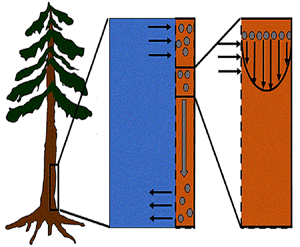
The physics of sucrose transport in plants, introduced in the early 1930s by the forestry scientist E. Münch (Münch Reference Münch1930), continues to be the workhorse model today, though this hypothesis is still not free from controversies (Curtis & Scofield Reference Curtis and Scofield1933; Spanner Reference Spanner1958; Christy & Ferrier Reference Christy and Ferrier1973; Fensom Reference Fensom1981; Lang Reference Lang1983; Thompson & Holbrook Reference Thompson and Holbrook2003a; Minchin & Lacointe Reference Minchin and Lacointe2005; Ryan & Asao Reference Ryan and Asao2014; Knoblauch & Peters Reference Knoblauch and Peters2017; Savage et al. Reference Savage, Beecher, Clerx, Gersony, Knoblauch, Losada, Jensen, Knoblauch and Holbrook2017; Huang et al. Reference Huang, Domec, Palmroth, Pockman, Litvak and Katul2018; Sevanto Reference Sevanto2018). The Münch hypothesis assumes that sucrose molecules produced during leaf photosynthesis in mesophyll cells are loaded into phloem tubes (figure 1a). Through osmosis, water is then pulled into the phloem from adjacent cells, or xylem vessels, creating a positive pressure that pushes water along the phloem tube towards sink tissues where sucrose is consumed or converted to other forms for storage (figure 1a). Because the sucrose concentration in these sink tissues is much smaller than in source tissues, the driving force for water movement in the phloem system can then be established. The elegance, plausibility, simplicity and partial experimental support gave this hypothesis a broad acceptance in plant physiology (Wardlaw Reference Wardlaw1974; Housley & Fisher Reference Housley and Fisher1977; Rand Reference Rand1983; van Bel Reference van Bel2003; Pickard & Abraham-Shrauner Reference Pickard and Abraham-Shrauner2009; Mencuccini & Hölttä Reference Mencuccini and Hölttä2010; Jensen et al. Reference Jensen, Lee, Bohr, Bruus, Holbrook and Zwieniecki2011; Knoblauch & Oparka Reference Knoblauch and Oparka2012; Nikinmaa et al. Reference Nikinmaa, Hölttä, Hari, Kolari, Mäkelä, Sevanto and Vesala2013; Jensen et al. Reference Jensen, Berg-Sørensen, Bruus, Holbrook, Liesche, Schulz, Zwieniecki and Bohr2016; Knoblauch et al. Reference Knoblauch, Knoblauch, Mullendore, Savage, Babst, Beecher, Dodgen, Jensen and Holbrook2016; Jensen Reference Jensen2018; Konrad et al. Reference Konrad, Katul, Roth-Nebelsick and Jensen2018).

Figure 1. (a) Water and sucrose transport in the phloem (orange) driven by water inflow from and back into the xylem (blue) from source (i.e. leaves) to sink (i.e. roots). (b) Schematic of the experiment used by Jensen et al. (Reference Jensen, Rio, Hansen, Clanet and Bohr2009) to describe sucrose transport (side and top views). The phloem geometry is assumed to be a long and narrow tube of length  $L$ and radius
  $a$. The xylem is assumed to be a naturally filtered water reservoir that surrounds the semipermeable tube. Sucrose enters the tube at
  $t = 0$ in a radially uniform manner and is axially described by a smooth function
  $f(x)$. Sucrose is conserved in the tube during the entire experiment because the tube top is closed (i.e. all sucrose molecules that enter the tube remain in the tube). The axial and radial coordinates as well as the boundary conditions used are shown.
The main critique of the Münch hypothesis, which continues to draw research interest even today, is whether such a driving force allows sucrose to be loaded and transported sufficiently quickly over long distances as may be expected in tall trees (Fensom Reference Fensom1981; Turgeon Reference Turgeon2010). The best estimates of sucrose concentrations in leaves raise some concerns about the generality and utility of the Münch hypothesis. It has been reported that sucrose concentration in some leaves of tall trees is smaller than in shorter vegetation (Fensom Reference Fensom1981; Turgeon Reference Turgeon2010). Such dependence of the concentration is not compatible with predictions that require the effective hydraulic conductivity to diminish with increased tube length (Knoblauch et al. Reference Knoblauch, Knoblauch, Mullendore, Savage, Babst, Beecher, Dodgen, Jensen and Holbrook2016; Knoblauch & Peters Reference Knoblauch and Peters2017; Savage et al. Reference Savage, Beecher, Clerx, Gersony, Knoblauch, Losada, Jensen, Knoblauch and Holbrook2017) assumed to be proportional to plant height.
The focus here is on the inclusion of Taylor dispersion, an overlooked mechanism that enhances the spread of solute in impermeable tubes (Taylor Reference Taylor1953). It will be shown that Taylor dispersion in osmotically driven flow such as the one described by the Münch hypothesis (i.e. tube walls are membranes) leads to further adjustments apart from the apparent increase in diffusion. The physics of those adjustments and their effects on phloem flow and sucrose transport rates are uncovered.
In the following sections, the system of equations that describe the physics of sucrose transport in plants is presented. The governing equations and their associated assumptions are first discussed. Next, the derivation of Taylor dispersion in osmotically driven flows is featured after area-averaging the governing equations. A brief description of the so-called Münch mechanism, which has been derived and reviewed elsewhere (Jensen et al. Reference Jensen, Rio, Hansen, Clanet and Bohr2009, Reference Jensen, Berg-Sørensen, Bruus, Holbrook, Liesche, Schulz, Zwieniecki and Bohr2016), is then presented while accommodating Taylor dispersion. Finally, a scaling analysis is used to demonstrate the existence of two distinct flow regimes based on the magnitude of the Münch number, which is defined as the ratio of the axial (mainly viscous) to membrane flow resistance (Jensen et al. Reference Jensen, Rio, Hansen, Clanet and Bohr2009, Reference Jensen, Berg-Sørensen, Bruus, Holbrook, Liesche, Schulz, Zwieniecki and Bohr2016). The focus of the results and discussion is on the consequences of Taylor dispersion on velocity and sucrose fluxes within these two ‘end-member’ flow regimes.
2. Theory
The basic equations describing sucrose transport in plants are first reviewed. Since the focus is on solute mass transport mechanisms, the conductive phloem geometry is simplified to permit analytical tractability (figure 1b). It is approximated by a long tube with length  $\textit {L}$ and radius
  $\textit {a}$ connecting sucrose production at the leaf with sinks anywhere in the tissues below the leaves such as in the roots (figure 1). The phloem sieve tubes are long and narrow, meaning that any dynamic scaling on flow variables will be subject to the slender geometry with aspect ratio
  $\epsilon = a / L\ll 1$.
The tube surface area is covered by a membrane with uniform permeability  $\textit {k}$ that allows water molecules, but not sucrose molecules, to be exchanged with the surrounding aqueous environment. Because the tube is effectively immersed in a water reservoir, the treatment of water flow can be achieved by placing the tube in a vertical position so that
  $x$ defines the longitudinal direction and
  $r$ defines the radial direction from the centre of the tube (figure 1b). In this representation, sucrose molecules enter the bottom of the tube at
  $x=0$ and propagate within the tube until
  $x=L$. The tube is closed at
  $x=L$.
Throughout, sucrose concentration is denoted as  $c$, fluid pressure as
  $p$, longitudinal velocity component as
  $u$, and radial velocity component as
  $v$. The
  $u$ value in plants is small, and therefore the flow can be approximated as a low-Reynolds-number flow, where the Reynolds number is defined as
  ${\textit {Re}}=2a u/\nu \ll 1$, with
  $\nu =\mu /\rho$ the kinematic viscosity, and
  $\mu$ and
  $\rho$ the dynamic viscosity and density of water, respectively. Hence, inertial effects in the longitudinal momentum balance can be ignored relative to viscous stresses. Frictional losses due to the presence of sieve plates within the phloem are also ignored, though, in some cases, this loss can be significant (Knoblauch et al. Reference Knoblauch, Knoblauch, Mullendore, Savage, Babst, Beecher, Dodgen, Jensen and Holbrook2016). This set-up does not reproduce all the geometric complexities of the phloem network in plants. The simplifications here are intended as a logical starting point for exploring Taylor dispersion in osmotically driven flow in idealized settings. The effects of these losses and the inhomogeneity produced due to the existence of sieve plates are left for future work.
For mass transport, the molecular Schmidt number  $Sc$, defined as
  $\nu / D$, where
  $D$ is the molecular diffusion coefficient, is large (
 $Sc >10\,000$ for sucrose in water). The fact that sucrose transport occurs at such a high
  $Sc$ implies that the advective transport term in the solute mass balance equation cannot be ignored (unlike in the momentum balance). The strength of solute advective to diffusive contributions are quantified using the Péclet number
  ${\textit {Pe}}=2a u/D$, which can also be expressed as
  ${\textit {Pe}} = {\textit {Re}} \, Sc$. While
  ${\textit {Re}}\ll 1$, the advective transport in the solute mass balance equation need not be small precisely because
  $Sc\gg 1$.
2.1. The governing equations
It is assumed that water is an incompressible Newtonian fluid with density  $\rho$ and viscosity
  $\mu$ satisfying the continuity equation
 \begin{equation} \frac{1}{r}\frac{{\partial} (r v)}{{\partial} r} + \frac{{\partial} u}{{\partial} x} = 0. \end{equation}
For very high  $c$,
$c$,  $\rho$ and
  $\mu$ need not be constant and can vary with
  $c$. However, for low
  $c$, this dependence can be ignored. Assuming cylindrical symmetry, the flow of water in the tube is described by momentum balance equations in the axial and radial directions:
 \begin{equation} \left.\begin{gathered} \rho \left( \frac{{\partial} u}{{\partial} t} + u \frac{{\partial} u}{{\partial} x} + v \frac{{\partial} u}{{\partial} r} \right) ={-} \frac{{\partial} p}{{\partial} x} + \mu \left[\frac{{\partial}^2 u}{{\partial} x^2} + \frac{1}{r}\frac{{\partial}}{{\partial} r}\left(r \frac{{\partial} u}{{\partial} r}\right)\right], \\ \rho \left( \frac{{\partial} v}{{\partial} t} + u \frac{{\partial} v}{{\partial} x} + v \frac{{\partial} v}{{\partial} r} \right) ={-} \frac{{\partial} p}{{\partial} r} + \mu \left[\frac{{\partial}^2 v}{{\partial} x^2} + \frac{1}{r}\frac{{\partial}}{{\partial} r} \left(r \frac{{\partial} v}{{\partial} r}\right) - \frac{v}{r^2}\right]. \end{gathered}\right\} \end{equation}
Equations (2.2) assume that there are no external forces on the fluid and that the gravitational forces are negligible (Thompson & Holbrook Reference Thompson and Holbrook2003a). The normalized variables defined by  $u = u_0 U$,
  $v = v_0 V$,
  $p = p_0 P$,
  $r = a R$ and
  $x = L X$ are introduced, where
  $u_0$,
  $v_0$ and
  $p_0$ are characteristic axial velocity, radial velocity and pressure. The characteristic length scales in the axial and radial dimensions are the tube length
  $L$ and radius
  $a$. The radial velocity scale
  $v_0 = \epsilon u_0$ is determined from the continuity equation, and
 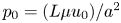 $p_0 = (L \mu u_0) / a^2$ is the viscous pressure scale.
The non-dimensional form for the fluid continuity is then
 \begin{equation} \frac{1}{R}\frac{{\partial} (R V)}{{\partial} R} + \frac{{\partial} U}{{\partial} X} = 0, \end{equation}
and the Navier–Stokes equations for the axial and radial velocities at steady state are
 \begin{equation} \left.\begin{gathered} {\textit{Re}} \,\epsilon \left(U \frac{{\partial} U}{{\partial} X} + V \frac{{\partial} U}{{\partial} R}\right) ={-} \frac{{\partial} P}{{\partial} X} + \epsilon^2\frac{{\partial}^2 U}{{\partial} X^2} + \frac{1}{R}\frac{{\partial}}{{\partial} R} \left(R \frac{{\partial} U}{{\partial} R}\right), \\ {\textit{Re}} \,\epsilon^3 \left(U \frac{{\partial} V}{{\partial} X} + V \frac{{\partial} V}{{\partial} R}\right) ={-} \frac{{\partial} P}{{\partial} R} + \epsilon^2 \left[\epsilon^2 \frac{{\partial}^2 V}{{\partial} X^2} + \frac{1}{R}\frac{{\partial}}{{\partial} R}\left(R \frac{{\partial} V}{{\partial} R}\right) - \frac{V}{R^2}\right]. \end{gathered}\right\} \end{equation}
As in lubrication theory, when the reduced Reynolds number tends to zero (i.e.  $\epsilon {\textit {Re}} {\rightarrow 0}$), the leading-order terms in (2.4) satisfy
 \begin{equation} \frac{1}{R}\frac{{\partial}}{{\partial} R}\left(R \frac{{\partial} U}{{\partial} R}\right) = \frac{{\partial} P}{{\partial} X},\quad \frac{{\partial} P}{{\partial} R} = 0. \end{equation}
The boundary conditions needed to obtain the leading-order term of the axial and radial velocities as a function of the pressure gradient inside the tube from (2.5a,b) are as follows:
 \begin{equation} U(R = 1) = 0,\quad \frac{\partial U}{\partial R}\bigg|_{R = 0} = 0,\quad V(R = 0) = 0. \end{equation}
The first boundary condition in (2.6a–c) states that the axial velocity within the membrane is zero (though the radial velocity is finite at  $R=1$ due to osmosis, as later discussed). The second and third boundary conditions are derived from symmetry considerations at the centre of the pipe.
Combining (2.5a,b) with the continuity equation (2.3) and imposing the aforementioned boundary conditions (2.6a–c), the axial and radial velocities are given by
 \begin{equation} U ={-} \frac{1}{4} \frac{{\partial} P}{{\partial} X} (1 - R^2 ), \quad V = \frac{1}{4} \frac{{\partial}^2 P}{{\partial} X^2} \left(\frac{R}{2} - \frac{R^3}{4} \right). \end{equation}
For completeness, these equations are also expressed in dimensional form as
 \begin{equation} u ={-} \frac{1}{4 \mu} \frac{{\partial} p}{{\partial} x} (a^2 - r^2 ), \quad v = \frac{1}{4 \mu} \frac{{\partial}^2 p}{{\partial} x^2} \left(\frac{a^2}{2} r - \frac{r^3}{4} \right). \end{equation}
Equation (2.8a,b) represents the velocity components variation as a first-order approximation in the limit of small reduced Reynolds number. A more general treatment can be found elsewhere (Aldis Reference Aldis1988). While the axial velocity profile is identical in mathematical form to the Hagen–Poiseuille (HP) equation derived for impermeable tubes, the radial velocity is not. In impermeable tubes, the no-slip condition at the pipe wall ( $R=1$) and symmetry considerations at the centre of the pipe (
 $R=0$) necessitate
  $v=0$ everywhere in the pipe, which is not the case here due to osmosis.
The use of the HP approximation to describe water movement in the phloem has been the subject of some debate (Weir Reference Weir1981; Phillips & Dungan Reference Phillips and Dungan1993; Henton et al. Reference Henton, Greaves, Piller and Minchin2002; Thompson & Holbrook Reference Thompson and Holbrook2003a, Reference Thompson and Holbrook; Jensen et al. Reference Jensen, Rio, Hansen, Clanet and Bohr2009, Reference Jensen, Berg-Sørensen, Friis and Bohr2012; Cabrita, Thorpe & Huber Reference Cabrita, Thorpe and Huber2013). The main cause of this debate has been the assumption of an externally imposed constant pressure gradient  ${\partial p}/{\partial x}$ routinely invoked in the conventional derivation of the HP equation (Phillips & Dungan Reference Phillips and Dungan1993). A constant
  ${\partial p}/{\partial x}$ requires
  ${\partial ^2 p}/{\partial x^2}=0$ and consequently
  $v=0$ everywhere (including at the boundary
  $r=a$). The expressions for
  $u$ and
  $v$ in (2.8a,b) are compatible with the HP assumptions of a force balance between pressure gradients and viscous stresses without requiring a constant
  ${\partial p}/{\partial x}$. In osmotically driven flow, the representation of the pressure and its gradients will be elaborated upon later. While the combination of the continuity equation and the two momentum balance equations provide three equations in three unknowns (
 $p$,
$p$,  $v$ and
  $u$), they remain incomplete because an additional boundary condition on
  $v$ at
  $r=a$ is required. This boundary condition must be supplied by Darcy's law and osmoregulation.
The conservation of solute mass, which adds one more unknown and one more equation for  $c$, is derived using the Reynolds transport theorem. The transport of sucrose in axial and radial directions follows from advection and molecular diffusion. The equation for the solute mass balance can be expressed as
 \begin{equation} \frac{{\partial} c}{{\partial} t} + \frac{{\partial} (u c)}{{\partial} x} + \frac{1}{r}\frac{{\partial} (r v c)}{{\partial} r} = D \frac{{\partial}^2 c}{{\partial} x^2} + D \frac{1}{r}\frac{{\partial}}{{\partial} r}\left(r \frac{{\partial} c}{{\partial} r} \right). \end{equation}
The initial condition is that at  $t = 0$ (and
  $x = 0$) sucrose enters the tube in a radially uniform manner. However, axially, an initial distribution
  $c = f(x)$ is prescribed that is the same as that used by Jensen et al. (Reference Jensen, Rio, Hansen, Clanet and Bohr2009) to ensure a smooth initial profile along the tube (figure 1b). Along the axial direction, a no-mass-flux condition at
  $x=L$ (the tube is closed at this end) and an externally specified uniform concentration at the source (
 $x=0$) are imposed. Along the radial direction, symmetry considerations provide one boundary condition as before, which is
  ${\partial c}/{\partial r}=0$ at
  $r=0$, and the no-flux-of-solutes condition at
  $r=a$ provides the second boundary condition, where
 \begin{equation} v c - D \frac{{\partial} c}{{\partial} r }= 0. \end{equation}
The no-flux-of-solutes condition ensures that the membrane allows for the exchange of water molecules but not sucrose.
As discussed before, another boundary condition is needed for  $v$ at
  $r=a$ to mathematically complete the problem formulation. The equation providing closure to both
  $c$ and
  $v$ arises from a pressure difference relation across the membrane. This equation describes the radial flow of water from the surrounding reservoir into the tube due to osmosis. This equation is best formulated as a boundary condition that relates the radial velocity
  $v$ to the driving gradient for water movement involving the fluid pressure
  $p$ and the osmotic potential (which varies with
  $c$) at
  $r = a$. It is given as a Darcy-type flow expression
  $v = k (p - \varPi _b)$ (Iberall & Schindler Reference Iberall and Schindler1973), where
  $k$ is the membrane permeability and
  $\varPi _b$ is the osmotic potential at the membrane (
 $r=a$). For small
  $c$, the van ’t Hoff relation (
 $\varPi = R_g T c$) can be used to relate the osmotic potential
  $\varPi$ to the sucrose concentration at the membrane (
 $c=c_b$ at
  $r=a$), leading to
 \begin{equation} \frac{v_b}{k} = p - R_g T c_b, \end{equation}
where  $R_g$ is the gas constant and
  $T$ is the absolute temperature (assumed constant throughout). Equation (2.11) provides the required boundary condition to link
  $v$ to
  $p$ and
  $c$, thereby providing the necessary closure for the problem. It is to be noted that, at high
  $c$, not only does the van ’t Hoff relation require modification but
  $\rho$,
  $\nu$ and
  $D$ also become dependent on
  $c$. This high-sucrose-concentration limit is outside the scope of the Taylor dispersion analysis featured next.
2.2. Taylor dispersion in osmotically driven flows
To elucidate the role of Taylor dispersion, (2.9) must be averaged over the cross-sectional area of the tube. The second term on the left-hand side, area-averaged  ${\partial }(\overline {u c})/{{\partial } x}$, is interesting, given its connection to the original work of Taylor and is now explored.
Even in impermeable tubes, this term is not  ${\partial } \bar {u} \bar {c}/{{\partial } x}$. As noted by Taylor (Reference Taylor1953), the interaction between velocity and concentration variations adds an apparent diffusion term labelled as dispersion. This dispersion term can be related to the ‘mixed’ Péclet number
  ${\textit {Pe}} = (u_0 a)/D$ that describes the influence of the axial velocity on radial variations of concentration. Its effect is to increase the apparent diffusion coefficient, and whence the name ‘Taylor dispersion’ (Taylor Reference Taylor1953). However, in osmotically driven flows, the radial component of the velocity appears due to osmosis. The finite radial velocity results in a ‘radial’ Péclet number
  $Pe_r = (v_0 a)/D$, which is the ratio of radial advection to radial diffusion. Both flows will also have an influence from the ‘axial’ Péclet number
  $Pe_l = (u_0 L)/D$ that describes the ratio of axial advection to axial diffusion. In this section, the new Taylor dispersion term is derived and its effect on osmotically driven flows for different limits of
  $Pe_r$ and
  $Pe_l$ is discussed. To arrive at expressions linking
  $\overline {u c}$ to
  $\bar {u} \bar {c}$, flow properties are decomposed into area-averaged and deviation components given as
  $c = \bar {c}(x,t) +\tilde {c}(x,r,t)$,
  $u = \bar {u}(x,t) + \tilde {u}(x,r,t)$ and
  $v = \bar {v}(x,t) + \tilde {v}(x,r,t)$, where
 \begin{equation} \bar{c} = \frac{2}{a^2}\int_0^a rc\,\mathrm{d}r, \end{equation}
and similarly for other quantities. The average of any deviation is identically zero.
Inserting the decomposed variables into (2.9) leads to
 \begin{align} & \bar{c}_t + \tilde{c}_t + (\bar{c} \bar{u})_x + (\bar{c} \tilde{u})_x + (\tilde{c} \bar{u})_x + (\tilde{c} \tilde{u})_x \nonumber\\ &\qquad + \frac{1}{r}(r\bar{c} \bar{v})_r + \frac{1}{r}(r\bar{c} \tilde{v})_r + \frac{1}{r}(r\tilde{c} \bar{v})_r + \frac{1}{r}(r\tilde{c} \tilde{v})_r \nonumber\\ &\quad = D \bar{c}_{xx} + D \tilde{c}_{xx} + D \frac{1}{r}(r \tilde{c}_r)_r + D \frac{1}{r}(r \bar{c}_r)_r, \end{align}
where differentiation is now written with respect to the subscripted variables. Averaging (2.13) radially while removing the last term on the right-hand side of the equation ( $\bar {c}$ only varies in
  $x$ and
  $t$), the area-averaged equation is
 \begin{align} & \frac{2}{a^2}\int_0^a r \bar{c}_t \, \mathrm{d} r + \frac{2}{a^2}\int_0^a r \tilde{c}_t \, \mathrm{d} r + \frac{2}{a^2}\int_0^a r (\bar{c} \bar{u} )_x \, \mathrm{d} r + \frac{2}{a^2}\int_0^a r (\bar{c} \tilde{u} )_x \, \mathrm{d} r \nonumber\\ &\qquad + \frac{2}{a^2}\int_0^a r (\tilde{c} \bar{u} )_x \, \mathrm{d} r + \frac{2}{a^2}\int_0^a r (\tilde{c} \tilde{u} )_x \, \mathrm{d} r + \frac{2}{a^2}\int_0^a (r \bar{c} \bar{v} )_r \, \mathrm{d} r \nonumber\\ &\qquad + \frac{2}{a^2}\int_0^a (r \bar{c} \tilde{v} )_r \, \mathrm{d} r + \frac{2}{a^2}\int_0^a (r \tilde{c} \bar{v} )_r \, \mathrm{d} r + \frac{2}{a^2}\int_0^a (r \tilde{c} \tilde{v} )_r \, \mathrm{d} r \nonumber\\ &\quad = \frac{2}{a^2}D\int_0^a (r \bar{c}_{xx} ) \, \mathrm{d} r + \frac{2}{a^2}D\int_0^a (r \tilde{c}_{xx} ) \, \mathrm{d} r + \frac{2}{a^2}D\int_0^a (r \tilde{c}_r )_r \, \mathrm{d} r. \end{align}
Eliminating terms that are the averages of deviations and evaluating other explicit integrals, (2.14) becomes
 \begin{equation} \bar{c}_t + (\bar{c} \bar{u})_x + \frac{2}{a^2}\int_0^a r (\tilde{c} \tilde{u} )_x \,\mathrm{d} r + \frac{2}{a}\left[c v - D \frac{{\partial} \tilde{c}}{{\partial} r}\right]_{r = a} = D \bar{c}_{xx}. \end{equation}
 The zero-mass-flux boundary condition at the membrane,  $v c - D\,{\partial } c/{\partial } r \vert _{r=a} = 0$, is enforced so that no sucrose molecules cross the membrane. Hence, the area-averaged equation satisfying this boundary condition (while noting that
  ${\partial } c/{\partial } r = {\partial } \tilde {c}/{\partial } r$) is
 \begin{equation} \bar{c}_t + (\bar{c} \bar{u})_x + \frac{2}{a^2}\int_0^a r (\tilde{c} \tilde{u} )_x \,\mathrm{d} r = D \bar{c}_{xx}. \end{equation}
To determine the contribution from the integral  $2{a^{-2}}\int _0^a r(\tilde {c} \tilde {u})_x \,\mathrm {d} r$, a separate equation for
  $\tilde {c}$ must be derived. This equation is obtained by subtracting (2.16) from (2.13) to yield
 \begin{align} & \tilde{c}_t + (\bar{c} \tilde{u} )_x + (\tilde{c} \bar{u} )_x + (\tilde{c} \tilde{u} )_x - \frac{2}{a^2}\int_0^a r (\tilde{c} \tilde{u} )_x \,\mathrm{d} r \nonumber\\ &\qquad + \frac{1}{r} (r \bar{c} \bar{v} )_r + \frac{1}{r} (r \bar{c} \tilde{v} )_r + \frac{1}{r} (r \tilde{c} \bar{v} )_r + \frac{1}{r} (r \tilde{c} \tilde{v} )_r \nonumber\\ &\quad = D \tilde{c}_{xx} + D\frac{1}{r}(r \tilde{c}_r)_r. \end{align}
 To proceed further analytically, additional simplifications to (2.17) must be invoked. It is first assumed that  $\tilde {c} \ll \bar {c}$, as earlier discussed. Next, a dominant balance argument is employed. The most important term on the right-hand side is
  $(1/r) (r \tilde {c}_r)_r$ because
  $(1/r) (r \tilde {c}_r)_r = \textit {O}(\tilde {c}/a^2) \gg \tilde {c}_{xx} = \textit {O}(\tilde {c}/L^2)$. Unlike impermeable tubes, this term must balance three dominant terms on the left-hand side rather than just one, where the two new terms are the result of osmosis (
 $v \neq 0$). These terms are the second, six and seventh, because all other terms are
  $\textit {O}(\tilde {c})$, which can be neglected when noting that
  $(1/r){\partial } (r \tilde {c} v)/{\partial } r = \textit {O}(\epsilon u \tilde {c}/a)$ (the sixth term can also be written as
  $\bar {c} \bar {v}/r$). This argument holds when assuming that the boundary layer near the membrane is negligible, as reasoned elsewhere (Pedley Reference Pedley1983; Aldis Reference Aldis1988; Jensen, Bohr & Bruus Reference Jensen, Bohr and Bruus2010; Haaning et al. Reference Haaning, Jensen, Hélix-Nielsen, Berg-Sørensen and Bohr2013) and the term
  $(\tilde {c} \tilde {u})_x$, which, even though averaged, remains smaller than
  $(\tilde {u} \bar {c})_x$. Hence, with these arguments, the dominant balance leads to a simplified and solvable equation for the sought
  $\tilde {c}$ given by
 \begin{equation} (\bar{c} \tilde{u} )_x + \bar{c} \frac{v}{r} + \bar{c} \tilde{v}_r = D\frac{1}{r}(r \tilde{c}_r)_r. \end{equation}
For the  $\tilde {u}$,
  $v/r$ and
  ${\partial } \tilde {v}/{\partial } r$ expressions, the result in (2.8a,b) can be used when noting that
  $\bar {u} = -(a^2(8\mu )^{-1}){\partial } p / {\partial } x$,
  $u = \bar {u}(2 - (2/a^2)r^2)$,
  $\bar {v} = -(7/15) a \bar {u}_x$ and
  $v = \bar {u}_x (r^3/(2a^2) - r)$. Hence,
  $\tilde {u}$,
  $v/r$ and
  ${\partial } \tilde {v}/{\partial } r$ can now be solved as functions of the area-averaged velocity as
 \begin{gather} \tilde{u} = u - \bar{u} = \bar{u}\left(1 - \frac{2}{a^2}r^2\right),\quad \tilde{u}_x = \bar{u}_x\left(1 - \frac{2}{a^2}r^2\right), \end{gather}
 \begin{gather}\frac{ v }{r} = \bar{u}_x\left(\frac{r^2}{2a^2} - 1\right), \quad \tilde{v}_r = \bar{u}_x\left(\frac{3}{2a^2}r^2 - 1\right). \end{gather}
 From this result, and noting that the area-averaged concentration is a function only of axial position and time, (2.18) is now separable in radial and axial positions and can be solved for  $\tilde {c}$ by integrating in r to obtain
 \begin{equation} \tilde{c} = \frac{1}{D}\bar{u}\bar{c}_x\left(\frac{r^2}{4} - \frac{1}{8 a^2}r^4\right) - \frac{1}{4D}\bar{u}_x\bar{c}r^2 + A(x,t)\ln{r} + B(x,t), \end{equation}
where A and B are integration constants to be determined. For the concentration to be bounded at  $r = 0$, it is required that
  $A = 0$. The area-averaged concentration deviation is zero by its definition (i.e.
  $\int _0^a (r\tilde {c})\,\mathrm {d} r = 0$) and leads to
  $B = (a^2/8D)\bar {u}_x\bar {c} - (a^2/12D)\bar {u}\bar {c}_x$. Hence,
  $\tilde {c}$ can be approximated as a function of the area-averaged concentration and axial velocity using
 \begin{equation} \tilde{c} = \frac{1}{D}\left(\frac{r^2}{4} - \frac{1}{8a^2}r^4 - \frac{a^2}{12}\right) \bar{u}\bar{c}_x+ \frac{1}{D} \left(-\frac{r^2}{4} + \frac{a^2}{8}\right)\bar{u}_x\bar{c}. \end{equation}
From the concentration deviation given in (2.21) and the velocity deviation given by (2.19a), the integral in (2.16) can now be determined to include the Taylor dispersion effect. After some algebra, the new form of the area-averaged equation for conservation of solute mass can be shown to reduce to
 \begin{equation} \frac{{\partial} \bar{c}}{{\partial} t} + \frac{{\partial}}{{\partial} x}\left[\left(1 + \frac{a^2}{24 D} \frac{{\partial} \bar{u}}{{\partial} x}\right)\bar{c} \bar{u}\right] = \frac{{\partial}}{{\partial} x} \left[\left(\frac{a^2 \bar{u}^2}{48 D} + D\right)\frac{{\partial} \bar{c}}{{\partial} x}\right]. \end{equation}
 Some features in (2.22) should be pointed out when comparing it to the impermeable tube case of Taylor dispersion. The conventional Taylor dispersion term  $(a\bar {u})^2/(48 D)$ is recovered on the right-hand side of (2.22). This term is always positive and must act to enhance the apparent diffusion coefficient. However, a new term emerges on the left-hand side of (2.22) that is absent in impermeable tubes. This term is responsible for transport into or out of the domain and depends on concentration gradients in the domain. Its sign is problem- and position-dependent because the mean velocity gradient can be either negative or positive depending on whether the flow is accelerating or decelerating.
The second equation needed to close the problem in the area-averaged form is (2.11). In this equation, the radial velocity v at  $r = a$ can be formulated from (2.8a,b) as a function of the area-averaged axial velocity,
  $v|_{r = a} = - (a/2)\bar {u}_x$. The concentration at the boundary
  $c_b$ can be approximated by the area-averaged concentration
  $\bar {c}$. This simplification ignores any boundary-layer effects at the membrane, though it abides by pragmatic considerations that
  $k$ is experimentally determined using averaged quantities when applying pressure and measuring the average axial velocity. The implication of this assumption is further discussed in appendix A. After differentiating in
  $x$ to relate the pressure term to the area-averaged axial velocity, (2.11) can be written in the following form:
 \begin{equation} R_g T \frac{{\partial} \bar{c}}{{\partial} x} = \frac{a}{2 k} \frac{{\partial}^2 \bar{u}}{{\partial} x^2} - \frac{8 \mu}{a^2}\bar{u}. \end{equation}
Equation (2.22) can be coupled with (2.23) to offer a new closed-form expression that describes axial sucrose transport in the phloem while accounting for Taylor dispersion.
3. Simplified model
The findings from (2.22) and (2.23) are now interpreted in the context of prior one-dimensional (axial) theories of phloem transport (Thompson & Holbrook Reference Thompson and Holbrook2003a; Jensen et al. Reference Jensen, Rio, Hansen, Clanet and Bohr2009; Huang et al. Reference Huang, Domec, Palmroth, Pockman, Litvak and Katul2018). Prior models commence with the assumption that  $\textit {v} \ll \textit {u}$ so that the momentum balance for
  $v$ can be omitted. Using this assumption, the area-averaged axial velocity is then directly related to the pressure gradient (for low
  ${\textit {Re}}$ and neglecting gravitational forces) by the HP approximation
 \begin{equation} \bar{u} ={-} a^2 (8 \mu)^{{-}1}\frac{{\partial} p}{{\partial} x}, \end{equation}
as shown in § 2.1 and discussed elsewhere (Thompson & Holbrook Reference Thompson and Holbrook2003a; Jensen et al. Reference Jensen, Rio, Hansen, Clanet and Bohr2009).
The flow through a membrane can be described using conservation of mass for a constant  $\rho$ around a small part of the tube length
  ${\rm \Delta} x$, where the osmotic potential and pressure potential are balanced to create an advection difference across
  ${\rm \Delta} x$ between inlet position
  $i$ and outlet position
  $i+1$ given as (Jensen et al. Reference Jensen, Rio, Hansen, Clanet and Bohr2009)
 \begin{equation} {\rm \pi}a^2 (\bar{u}_{i+1} - \bar{u}_{i}) + 2 {\rm \pi}a {\rm \Delta} x \, k (\varPi - p) = 0. \end{equation}
As before, for small  $c$, the van ’t Hoff relation
  $\varPi = R T \bar {c}$ can be used to relate the osmotic potential
  $\varPi$ to
  $\bar {c}$. Taking the limit
  ${\rm \Delta} \textit {x}{\rightarrow 0}$, a relation between
  $\bar {c}$,
  $\bar {u}$ and
  $p$ can now be derived and is given by
 \begin{equation} \frac{a}{2} \frac{{\partial} \bar{u}}{{\partial} x} = k (R_g T \bar{c} - p). \end{equation}
Using (3.1),  $p$ can be eliminated, resulting in an equation that is the same as (2.23) as derived from the boundary condition (2.11) in § 2.2.
To mathematically close the problem, the area-averaging operation can be applied to the advection–diffusion equation (2.9), which upon setting  $\overline {uc} = \bar {u} \bar {c}$ leads to
 \begin{equation} \frac{{\partial} \bar{c}}{{\partial} t} + \frac{{\partial} \bar{u} \bar{c}}{{\partial} x} = D \frac{{\partial}^2 \bar{c}}{{\partial} x^2}. \end{equation}
This resulting transport equation is different from (2.22) due to the approximation  $\overline {uc} \approx \bar {u} \bar {c}$. This latter approximation, which ignores Taylor dispersion, has been used extensively in prior representation of sucrose transport in the phloem (Thompson & Holbrook Reference Thompson and Holbrook2003a; Jensen et al. Reference Jensen, Berg-Sørensen, Friis and Bohr2012, Reference Jensen, Berg-Sørensen, Bruus, Holbrook, Liesche, Schulz, Zwieniecki and Bohr2016; Huang et al. Reference Huang, Domec, Palmroth, Pockman, Litvak and Katul2018). Its consequence is that area-averaged quantities also satisfy the same solute conservation equation. The inclusion of Taylor dispersion (i.e. arising from
  $\overline {uc} \neq \bar {u} \bar {c}$) in the aforementioned system of equations and tracking its consequences on sucrose front speed frames the scope of the work presented here.
4. Non-dimensional form for both models
This section presents the non-dimensional form for the simplified model derived by Jensen et al. (Reference Jensen, Rio, Hansen, Clanet and Bohr2009) and discussed in § 3 and the model that includes Taylor dispersion derived in § 2.2. Because the non-dimensional forms are used to construct model runs for the discussion, they are featured here for convenience.
4.1. Non-dimensional form of the simplified model
Choosing the following scaling for the concentration, velocity, length and time,  $c = c_0 C$ (
 $c_0$ being the initial concentration released at
  $x=0$),
  $u = u_0 U$,
  $x = L X$ and
  $t = t_0 \tau$, equations (2.23) and (3.4) can be made non-dimensional and given by
 \begin{gather} \frac{{\partial} C}{{\partial} X} = \frac{{\partial}^2 U}{{\partial} X^2} - M U, \end{gather}
 \begin{gather}\frac{{\partial} C}{{\partial} \tau} + \frac{{\partial} U C}{{\partial} X} = \frac{1}{Pe_l} \frac{{\partial}^2 C}{{\partial} X^2}, \end{gather}
where  $t_0 = L u_0^{-1}$ is the advection time scale,
  $u_0 = 2 k R_g T c_0 L a^{-1}$ is the advection velocity,
  $M = 16 \mu L^2 k a^{-3}$ is the Münch number, which describes the forces responsible for the axial variation of
  $\bar {c}$ (Jensen et al. Reference Jensen, Rio, Hansen, Clanet and Bohr2009), and
  ${\textit {Pe}}_l = u_0 L/D$ is the Péclet number in the axial direction, which can be significant for high
  $Sc$ even when
  $u_0$ is small. It is to be noted that this non-dimensional number is the inverse of
  $\bar {D}$ used by Jensen et al. (Reference Jensen, Rio, Hansen, Clanet and Bohr2009).
In the limiting case where  $M$ is very large, the non-dimensional variable
  $U$ in (4.1a) can be rescaled by
  $M$ to yield
 \begin{gather} \frac{{\partial} C}{{\partial} X} = \frac{1}{M}\frac{{\partial}^2 \hat{U}}{{\partial} X^2} - \hat{U}, \end{gather}
 \begin{gather}\frac{{\partial} C}{{\partial} \tau} + \frac{1}{M}\frac{{\partial} \hat{U}C}{{\partial} X} = \frac{1}{{\textit{Pe}}_l}\frac{{\partial}^2 C}{{\partial} X^2}, \end{gather}
where  $U = \hat {U}/M$ and
  $\hat {U} = \textit {O}(1)$. When
  $M{\rightarrow \infty }$, the leading-order axial velocity becomes entirely driven by the mean concentration gradient (
 $\hat {U} = - {\partial } C/{\partial } X$). The analytical solution (when
  $M^{-1}C \gg 1/{\textit {Pe}}_l$) for this equation can be found elsewhere (Jensen et al. Reference Jensen, Rio, Hansen, Clanet and Bohr2009) and follows well-established methods for solving such nonlinear diffusion problems (King & Please Reference King and Please1986).
4.2. Non-dimensional form of the Taylor dispersion model
Using the same scaling analysis, (2.23) is not affected by the derivation of the Taylor dispersion (as expected). However, the non-dimensional form for the conservation of solute mass must be revised to include the radial Péclet number  ${\textit {Pe}}_r$. This revision yields
 \begin{equation} \frac{{\partial} C}{{\partial} \tau} + \frac{{\partial}}{{\partial} X}\left[\left(1 + \frac{{\textit{Pe}}_r}{24} \frac{{\partial} U}{{\partial} X}\right)U C\right] = \frac{{\textit{Pe}}_r}{48} \frac{{\partial}}{{\partial} X} \left[\left(U^2 + \frac{48}{{\textit{Pe}}_r {\textit{Pe}}_l}\right)\frac{{\partial} C}{{\partial} X}\right], \end{equation}
where the scaling for the time  $t_0$ is the same as in § 4.1. The non-dimensional number
  ${\textit {Pe}}_r = a v_0/D$ defines a radial Péclet number, where
  $v_0 = \epsilon u_0$, with
  $\epsilon = a/L$, as expected from the continuity equation (2.1) in § 2.1. The non-dimensional number
  $48 {\textit {Pe}}_l^{-1} {\textit {Pe}}_r^{-1}$ can also be written as
  $48 (\epsilon {\textit {Pe}}_l)^{-2}$, since
  ${\textit {Pe}}_r = \epsilon ^2 {\textit {Pe}}_l$. This non-dimensional number is always much smaller than unity (i.e.
  $48 (\epsilon {\textit {Pe}}_l)^{-2} \ll \textit {O}(1)$) since axial advection is much bigger than axial diffusion (
 ${\textit {Pe}}_l \gg \textit {O}(1)$, as shown in table 3), which will lead to
  $\epsilon {\textit {Pe}}_l \gg \textit {O}(1)$. However, the non-dimensional radial Péclet number
  ${\textit {Pe}}_r/24$ can be large (
 $>$1 when radial advection dominates) or small (
 $\ll$1 when radial diffusion dominates) depending on the problem and will affect the overall sucrose transport time scale.
As before, in the limiting case where  $M$ is very large, the axial velocity can be rescaled by
  $M$. In this case, using the following change of variable for the axial velocity,
  $U = \hat {U}/M$, where
  $\hat {U} = \textit {O}(1)$, (4.3) can be written in the following form:
 \begin{equation} \frac{{\partial} C}{{\partial} \tau} + \frac{{\partial}}{{\partial} X}\left[\left(\frac{1}{M} + \frac{{\textit{Pe}}_r}{24 M^2}\frac{{\partial} \hat{U}}{{\partial} X}\right)\hat{U} C\right] = \frac{{\textit{Pe}}_r}{48}\frac{{\partial}}{{\partial} X}\left[\left(\frac{1}{ M^2}\hat{U}^2 + \frac{48}{{\textit{Pe}}_r {\textit{Pe}}_l}\right)\frac{{\partial} C}{{\partial} X}\right]. \end{equation}
For this case, the order of magnitude of the non-dimensional number  ${\textit {Pe}}_r/(24 M^2)$ will reveal the significance of the new terms in this model. In the results section, the Taylor dispersion effect for the cases of small to intermediate Münch number (
 $M \ll 1$ or
  $M =O(1)$) and large Münch number (
 $M{\rightarrow \infty }$) are presented.
5. Results
The results are divided into two parts. In the first part, a comparison of both the simplified model and the model including Taylor dispersion with published laboratory experiments (Jensen et al. Reference Jensen, Rio, Hansen, Clanet and Bohr2009) is carried out. These experiments are in the low-Münch -number regime. From this comparison, indirect evidence of the importance of Taylor dispersion in osmotically driven flows is established. The second part primarily focuses on the role of the new term (the radial Péclet number,  ${\textit {Pe}}_r$), primarily because
  $48 {\textit {Pe}}_r^{-1} {\textit {Pe}}_l^{-1} \ll \textit {O}(1)$. That is, molecular diffusion is smaller than the dispersion coefficient for typical phloem dimensions. In each
  $M$ limit, the behaviour of the flow is discussed depending on
  ${\textit {Pe}}_r$. The work here explores the flow properties and initial conditions affecting the behaviour of the sucrose concentration front shape traversing the tube. Flows characterized by small or negligible
  $M$(
$M$( $\ll 1$) are labelled as HP-driven flows, whereas flows characterized by very large
  $M$ are labelled as osmotically driven flows. To be clear, both flow regimes are osmotically driven – and such labelling simply reflects the roles of a fluid property
  $\mu$ and a membrane property
  $k$ on the relative magnitudes of the two terms in (2.23). Further details about the consequences of large or small
  $M$ on the scaling of
  $p$ is featured in appendix B for completeness.
5.1. Comparisons with published experiments
Indirect evidence for the significance of Taylor dispersion in osmotically driven laminar flow is presented based on published experiments. The data used here were extracted from an experiment described elsewhere (Jensen et al. Reference Jensen, Rio, Hansen, Clanet and Bohr2009) where  $M \sim 10^{-8}$. In this experiment, the authors compared an analytical solution derived for very small M and
  $\bar {D} = 1/{\textit {Pe}}_l$ with measurements without including Taylor dispersion in their model.
5.1.1. Experimental set-up
The experiment consisted of a tube with  $L = 30$ cm and radius
  $a = 0.5$ cm, with semipermeable membrane walls to allow water but not sucrose to be exchanged with the tube. This tube was placed vertically in a water reservoir, where the gravitational forces can be assumed to be negligible compared to the pressure gradient. This set-up, shown in figure 1(b), was used for five experimental runs in which osmotic pressure and
  $L$ were varied. The reported constant values for the dynamic viscosity and molecular diffusion in these experiments were
  $\mu = 1.5 \times 10^{-3}$ Pa s and
  $D = 6.9 \times 10^{-11}$ m
 $^2$ s
 $^{-1}$. Table 1 summarizes the different parameters for the five runs. In all five runs, the two non-dimensional numbers
  $M$ and
  $\bar {D}$ (
 ${=}1/{\textit {Pe}}_l$) are small (
 $M \sim 10^{-8}$ and
  $\bar {D} \sim 10^{-5}$) and are neglected in (4.1a) and (4.1b). In the absence of Taylor dispersion, this approximation allowed an analytical result to be derived for the mean concentration front position
  $x_f(t)$ given by (Jensen et al. Reference Jensen, Rio, Hansen, Clanet and Bohr2009)
 \begin{equation} \frac{x_f}{L} = 1 - \left(1-\frac{l}{L}\right)\exp\left(-\frac{t}{t_0}\right), \end{equation}
where  $l$ is the initial front height at
  $t=0$ and
  $t_0 = a (2 k R_g T \hat {c})^{-1} = a (2 k \varPi )^{-1}$.
Table 1. Published (Jensen et al. Reference Jensen, Rio, Hansen, Clanet and Bohr2009) experimental conditions for the five runs analysed here. The reported  $R_g T = 0.1$ bar (mM)
 $^{-1}$.

Figure 2 shows the relative front position  $(L - x_f)/(L - l)$ as a function of
  $t$ for the five runs. Equation (5.1) was used to compare the result of Jensen et al. (Reference Jensen, Rio, Hansen, Clanet and Bohr2009) with the experiment. It is to be noted that, in this equation, the reported radius
  $a$ and length
  $L$ as well as the permeability
  $k$ are in principle constants and the only variable that changes from one run to another was the osmotic potential, which was reported in table 1. To fit their analytical result from (5.1) to experiments using their reported osmotic potential, different values for membrane permeability were needed. These values are shown in table 2. To be clear, the low velocities across the membrane should yield a constant permeability
  $k$ (i.e. no Forchheimer correction is required, meaning the assumptions to use Darcy-type flow for (2.11) are still valid). Inspecting runs 1 and 4 in table 2, we can see that we have the same value for
  $k$ even when the osmotic potential is larger. The need to vary
  $k$ across runs led to the conjecture that the term
  $\overline {(cu)}_x$ may not be
  $(\bar {c}\bar {u})_x$ and Taylor dispersion may have some impact on this experiment. Other combinations can be formulated by changing the osmotic potential for each run while changing the permeability. However, no other combination led to a constant permeability for all the five runs. For this reason, we use these values for the model in the following section.

Figure 2. Log plot for the relative front position as a function of time  $t$ for the measured concentration (dashed line) and the analytical result given by Jensen et al. (Reference Jensen, Rio, Hansen, Clanet and Bohr2009) for the low-M limit (solid line) for the five different experimental runs listed in table 2.
Table 2. Different  $k$ values needed to match the analytical solution to measurements for each run in figure 2.

5.1.2. Data–model comparisons
From § 5.1.1, different values of  $k$ were necessary to fit the published analytical solution to the measurements for each run. In this section, the model for
  $x_f(t)$ that includes Taylor dispersion is now used to fit the data but using a single
  $k$ value across runs. For both models, the permeability
  $k$ was set to a constant
  $k = 0.8 \times 10^{-10}$ cm (Pa s)
 $^{-1}$, which yielded the best fit for all runs when Taylor dispersion was included (figure 3).

Figure 3. Log plot for the relative front position as a function of time for the experiments (crosses), analytical model for the low-M limit (dashed line) and Taylor dispersion (solid line) using a single value  $k = 0.8 \times 10^{-10}$ cm (Pa s)
 $^{-1}$. The last panel shows the concentration profile for the fifth run as a function of the axial position for the simplified model developed by Jensen et al. (Reference Jensen, Rio, Hansen, Clanet and Bohr2009) (dashed line) and the Taylor dispersion model proposed here (solid line). The inclusion of Taylor dispersion increases the front speed.
The Taylor dispersion model agrees with measurements for four out of the five runs (figure 3). Only the second run did not agree well with the proposed model for this  $k$ value at early times. One possible explanation for this discrepancy is that the measured osmotic potential may have been reported incorrectly since it is related to the mean concentration
  $\hat {c}$ by
  $\varPi = R_g T \hat {c}$ (published
  $R_g T = 0.1$ bar (mM)
 $^{-1}$ for all runs). From table 1, when the lower limit for
  $\hat {c} = 2.07$ mM and the upper limit for the osmotic pressure
  $\varPi = 0.16$ bar are used, the van ’t Hoff relation appears not to be satisfied with published
  $R_g T = 0.1$ bar (mM)
 $^{-1}$. The osmotic pressure should have attained a higher value, which can increase the osmotic driving force, leading to a faster flow and rapid
  $x_f$ advancement at early times. When revising the driving osmotic pressure to be compatible with the concentration, the agreement with the proposed model here is satisfactory (not shown).
The last plot of figure 3 presents the axial mean concentration for the fifth run at different times. The addition of Taylor dispersion leads to a different shape (not characterized by a front-like behaviour) at small time scales. As shown in figure 3, the longitudinal mean concentration variation of the Taylor dispersion model is different from the typical wave equation expected at the low- $M$ limit. At earlier times, the concentration does not advance with a sharp front because of the highly diffusive behaviour at early times. However, at later times, the concentration recovers the expected wave-like front.
In figure 4, the relative front position extracted from the data is plotted against the relative front position calculated from the two different models (circles for the Taylor dispersion model and crosses for Jensen's model) for the five different runs using a single  $k$ value,
  $k = 0.8 \times 10^{-10}$ cm (Pa s)
 $^{-1}$. The one-to-one line is shown as a solid line. The Taylor dispersion model provides a better fit with less scatter than that derived without Taylor dispersion. As expected, the relative front position for the second run does not lie on the one-to-one line for reasons related to the published osmotic potential value earlier noted.

Figure 4. Published data for the relative front position extracted by us from Jensen et al. (Reference Jensen, Rio, Hansen, Clanet and Bohr2009) as a function of the relative front position calculated from the two different models for the five runs. Black circles represent the Taylor dispersion model (derived here) and grey crosses represent the analytical approximation as derived by Jensen et al. (Reference Jensen, Rio, Hansen, Clanet and Bohr2009) for  $k = 0.8 \times 10^{-10}$ cm (Pa s)
 $^{-1}$.
5.2. Results of the models in both regimes
The effects of Taylor dispersion over a broader range of conditions than those covered by the experiments are now discussed. This discussion is centred on a comparison between the formulation that retains Taylor dispersion and the standard approach that ignores it. In appendix C, a comparison between these two models and a model that ignores the advection term while maintaining the original Taylor dispersion term as a local effect will be presented as well to describe the effect of the advection term on the flow.
Now, when designing a broad range of flow conditions (for the finite- ${\textit {Pe}}_r$ representation), it is imperative to assess how high
  ${\textit {Pe}}_r$ can be reached without violating the simplifications to the Navier–Stokes equations (2.2). To do so, it is assumed that the highest order of magnitude that the reduced
  ${\textit {Re}}$ (i.e.
  $\epsilon {\textit {Re}}$) can reach is
  $\textit {O}(10^{-2})$. The non-dimensional numbers
  $\epsilon {\textit {Re}}$ and
  ${\textit {Pe}}_r$ can be written as
  $\epsilon {\textit {Re}} = \epsilon \rho u_0 a/\mu = \rho v_0 a/\mu$ and
  ${\textit {Pe}}_r = v_0 a/D$. This leads to
  $v_0 a = (\mu /\rho ) \epsilon {\textit {Re}} = (\mu /\rho ) \textit {O}(10^{-2})$, which means that the highest
  ${\textit {Pe}}_r$ is
  $v_0 a/D = \mu (\rho D)^{-1} \textit {O}(10^{-2})$. Inserting the values for
  $\rho$,
  $\mu$ and
  $D$, the highest order of magnitude for
  ${\textit {Pe}}_r$ that can be sustained without the addition of inertial terms in the Navier–Stokes equations is
  $\textit {O}(10)$. This result implies that the radial advection can be equal to or higher than the radial diffusion. Obviously, with such high radial advection, the osmotic efficiency might be overestimated (Aldis Reference Aldis1988). The implication of this assumption is further discussed in appendix A.
5.2.1. Results for HP-driven flows
For this type of flow, the axial pressure gradient is the main driving force and is scaled by viscous forces, hence the name HP-driven flow. It either dominates or has similar importance as the osmotic potential. As discussed in § 4.1, M is finite (or  $M{\rightarrow 0}$) and the velocity is scaled by the boundary condition, which, as shown in appendix B, results in
  $u_0 = 2 k R_g T c_0 L a^{-1}$. For this case, the two dimensionless numbers in equation (4.3) for the conservation of solute mass can be written in the following forms:
  ${\textit {Pe}}_r = 2 k R_g T c_0 a D^{-1}$ and
  ${\textit {Pe}}_l = 2 k R_g T c_0 L^2 a^{-1} D^{-1}$.
In this section, the effect of  ${\textit {Pe}}_r$ for the HP-driven regime will be presented. The case where
  ${\textit {Pe}}_r$ is very small forms a logical starting point for discussion. Its effect on the flow when it reaches the aforementioned upper limit is then analysed. To do so, a numerical solution is obtained for both models. For the Taylor dispersion model, the system of equations solved is (4.3) and (4.1a). For the simplified model, it is (4.1b) and (4.1a).
In the case where  ${\textit {Pe}}_r \gg \epsilon$ (i.e.
  ${\textit {Pe}}_r \gg 1 / {\textit {Pe}}_l$), the molecular diffusion compared to the dispersion due to advection can be neglected and the non-dimensional form of equation (4.3) for solute mass conservation can be written as
 \begin{equation} \frac{{\partial} C}{{\partial} \tau} + \frac{{\partial}}{{\partial} X}\left[\left(1 + \frac{{\textit{Pe}}_r}{24} \frac{{\partial} U}{{\partial} X}\right)U C\right] = \frac{{\textit{Pe}}_r}{48}\frac{{\partial}}{{\partial} X}\left[U^2 \frac{{\partial} C}{{\partial} X}\right]. \end{equation}
From (5.2), the effect from Taylor dispersion decreases when  ${\textit {Pe}}_r {\rightarrow 0}$. At this limit, the equation exhibits similar behaviour to that derived in (4.1b) in § 4.1, but with two adjustments:
  $1/{\textit {Pe}}_l$ and
  ${\textit {Pe}}_r/48$ now have different orders of magnitude and the diffusion term itself is different. To illustrate the difference, a set of variables and initial conditions have been selected as presented in table 3.
Table 3. List of initial conditions and non-dimensional numbers for the four different cases discussed. All time scales are advection time scales (including the cases for high  ${\textit {Pe}}_r$).

From figures 5(a) and 5(b), the effect of Taylor dispersion on front speed appears small. The main difference can be seen in figure 5(a), where the front shape is smoother with the inclusion of Taylor dispersion. As mentioned before, the reason behind this ‘extra’ smoothing is the new dispersion term, and its order of magnitude is larger than molecular dispersion (i.e.  ${\textit {Pe}}_r/48 \sim \textit {O}(10^{-3}) \gg 1/{\textit {Pe}}_l \sim \textit {O}(10^{-6})$).

Figure 5. Results of the numerical solution for low  $M$ (first and second cases in table 3). (a,b) The low-
 ${\textit {Pe}}_r$ case for the time evolution of the concentration and velocity profiles. (c,d) The high-
 ${\textit {Pe}}_r$ case for the time evolution of the concentration and velocity profiles. Solid lines denote the result with Taylor dispersion and dashed lines denote the result without Taylor dispersion.
The second case of interest is high  ${\textit {Pe}}_r$. For this type of flow, advection is large enough to introduce a new behaviour in the flow. Assuming that the only variables that can be conveniently changed in an experiment are the dimensions of the tube (i.e. radius a and length L), its property (i.e. the permeability k) and the initial condition (i.e. initial concentration
  $c_0$), the set of variables chosen for illustration are shown in table 3.
This flow exhibits a different shape from the previous illustration. In this case, the advection term (from the analysis in § 2.2) is of the same magnitude as the original advection term and the dispersion term is of order  $\textit {O}(1)$. From figures 5(c) and 5(d), a finite
  ${\textit {Pe}}_r$ alters the behaviour of the flow, and the shape of the advancing concentration front disappears. From figure 5(c), it is also evident that, when including Taylor dispersion, the concentration front will sense the ‘end of the tube’ (downstream conditions) before the case where no Taylor dispersion is present. In this case, the advection term due to Taylor dispersion is larger than the original advection term (i.e.
  $U_X {\textit {Pe}}_r / 24 > 1$), leading to a higher front speed.
5.2.2. Results for osmotically driven flows
For this type of flow, the pressure can be scaled by the osmotic potential (as shown also in appendix B), hence the name osmotically driven flows. However, to maintain the same scaling for the velocity and pressure as for the case of low  $M$, the axial velocity
  $U$ can be rescaled by
  $M$ as discussed in § 4.1. In this case, the system of equations used to obtain the numerical solution is (4.4) and (4.2a) for the Taylor dispersion model, while (4.2b) and (4.2a) were used for the simplified model. As in § 5.2.1, the discussion on the effect of
  ${\textit {Pe}}_r$ on this type of flow will be presented. The non-dimensional form for the solute mass is the same as (4.4). However, to illustrate the importance of Taylor dispersion, the new non-dimensional form can be written using the linear relation between velocity and concentration for very high M discussed in § 4.1. This non-dimensional form is given as
 \begin{equation} \frac{{\partial} C}{{\partial} \tau} = \frac{{\partial}}{{\partial} X}\left[\left[ \frac{{\textit{Pe}}_r}{48 M^2} \left(\frac{{\partial} C}{{\partial} X}\right)^2 + \frac{1}{{\textit{Pe}}_l} + \left(\frac{1}{M} - \frac{{\textit{Pe}}_r}{24 M^2} \frac{{\partial}^2 C}{{\partial} X^2}\right) C\right]\frac{{\partial} C}{{\partial} X}\right], \end{equation}
From (5.3), the importance of the new terms resulting from Taylor dispersion can be shown by varying  ${\textit {Pe}}_r/M^2$. In this case,
  $M$ will be fixed (
 $M \sim \textit {O}(10^2)$) and
  ${\textit {Pe}}_r$ will be varied from small (i.e
  ${\textit {Pe}}_r \ll 1$) to its maximum limit (i.e.
  $\textit {O}(10)$).
For the low- ${\textit {Pe}}_r$ limit case, the tube properties and initial conditions, chosen to model this behaviour, are shown in table 3. As expected, one can see from figures 6(a) and 6(b) that both models behave approximately the same. The small value for
  ${\textit {Pe}}_r/M^2$ implies that both models have the same leading-order solution, which was discussed in § 4.1. One possible difference can be the shape of the moving solute front when
  $M^{-1}C \ll 1/{\textit {Pe}}_l$, where, in this model, the new Taylor dispersion terms can have a higher order of magnitude in this region. However, this analysis is tangential to the role of Taylor dispersion in the phloem and is better left for a future enquiry.

Figure 6. Results of the numerical solution for high  $M$ (third and fourth cases in table 3). (a,b) The low-
 ${\textit {Pe}}_r$ case for the time evolution of the concentration and velocity
  $\hat {U} = M U$ profiles. (c,d) The high-
 ${\textit {Pe}}_r$ case for the time evolution of the concentration and velocity
  $\hat {U} = M U$ profiles. Solid lines denote the result with Taylor dispersion and dashed lines denote the result without Taylor dispersion as before.
As in § 5.2.1, the interesting case is the higher  ${\textit {Pe}}_r$. For this reason, the set of initial and geometrical conditions, shown in table 3 with the resulting
  ${\textit {Pe}}_r$ and
  $\epsilon {\textit {Re}}$, are chosen for illustration. In figures 6(c) and 6(d), the large dispersion term has appreciably smoothed the mean longitudinal velocity and concentration along
  $x$. Another interpretation for the effect of Taylor dispersion can be seen from the longitudinal concentration distribution in figure 6(c), where the two plots differ in behaviour within the vicinity of the solute moving front. The reason for this difference is evident from (5.3), where the time derivative of the area-averaged concentration along
  $x$ is dependent on two new terms due to Taylor dispersion (advection and diffusion), unlike the case in the simplified model that depends on a constant term. A simplification can be achieved using an asymptotic analysis for most of the domain, which ultimately leads to a diffusion coefficient that depends on concentration
  $C$ only as discussed elsewhere (Jensen et al. Reference Jensen, Rio, Hansen, Clanet and Bohr2009). However, for the moving solute front, the other terms can be more important. From figures 6(c) and 6(d), the addition of Taylor dispersion speeds up the self-similar solution compared to the simplified model.
In this type of flow, the axial velocity  $U$ scales as
  $\textit {O}(1/M)$. This means that the radial advection is always much smaller than the radial diffusion even for the case where
  ${{\textit {Pe}}_r > 1}$. For this reason, when
  $M \gg 1$, the effect of Taylor dispersion decreases. However, in appendix D, a scaling analysis will show how the radial Péclet number can have a bigger effect if one uses a new scaling for the axial velocity as discussed in appendix B for the case where
  $M \gg 1$.
The difference in dynamics for both flows can be understood from comparing (5.2) for small  $M$ and (5.3) for large
  $M$. The transport described by (5.2) is significantly different in terms of having an advective term, while (5.3) is a nonlinear diffusion model with a diffusion coefficient that depends on the concentration and its derivatives. This apparent diffusion coefficient results from the linear relation between the velocity and the concentration (i.e.
  $\hat {U} = - {\partial } C/{\partial } X$) as a first-order approximation. It is the outcome of molecular diffusion, typical Taylor dispersion and the advection terms.
5.3. Model applicability in reference to sucrose transport in plants
In this section, the effect of Taylor dispersion on sucrose transport in phloem is discussed. As shown before, the effect of Taylor dispersion is solely related to  ${\textit {Pe}}_r$, which arises from the radial inflow of water due to osmosis. This radial Péclet number can be written as
  ${\textit {Pe}}_r = 2 k R_g T c_0 a D^{-1}$ to illustrate the different parameters that affect its significance in the area-averaged solute balance. Based on typical phloem values (Thompson & Holbrook Reference Thompson and Holbrook2003a), this non-dimensional number is small (i.e.
  ${\textit {Pe}}_r \ll \textit {O}(1)$), meaning that the Taylor dispersion effects will be more diffusive than increasing the speed of sucrose transport. Another limitation of this theory is the simplified geometry of the tube noted in the introduction. Real phloem tubes consist of series of small sieve elements connected by porous sieve plates. To accommodate these porous sieve plates, the pointwise Navier–Stokes equations must be revised to include a blockage term for the solid component of the plate (no velocity) whereas the porous part allows the flow to occur (with a velocity speedup to conserve the flow rate). In lieu of this treatment, the area-averaged Navier–Stokes equations may be amended by including a drag force with a drag coefficient that depends on the bulk Reynolds number upstream of the plate and a frontal area that is related to the solid space of the plate obstructing the flow. In either treatment, the effect of these plates on Taylor dispersion remains an open problem.
Thompson & Holbrook (Reference Thompson and Holbrook2003a) showed that head losses due to the presence of sieve plates may be included as reduced effective hydraulic conductivity of the sieve tube by adding a reduction factor. This treatment implies that the drag force from the plate can be replaced by an equivalent sidewall shear stress, thereby ignoring the disturbance the plate creates on the radial velocity and concentration distribution. Jensen et al. (Reference Jensen, Berg-Sørensen, Bruus, Holbrook, Liesche, Schulz, Zwieniecki and Bohr2016) and Thompson & Holbrook (Reference Thompson and Holbrook2003a) showed that, for low-Reynolds-number flows, the distance needed to recover the parabolic profile for  $u$ starting from a radially uniform velocity is
  $l_p < a$. The spacing of sieve elements
  $l_{sp}$ can be small to moderate (
 $10^{2}$ to
  $10^{3}$
  $\mathrm {\mu }$m for plants), while
  $a$ can vary from
  $10$ to
  $100$
$100$  $\mathrm {\mu }$m in plants. It can be surmised that there are situations where sieve plates introduce local (and minor) distortions to the existing analysis when
  $l_p/l_{sp} \ll 1$. Evidently, there are situations where
  $0.1<l_p/l_{sp}<1$ and the effect of Taylor dispersion predicted here is overestimated. In these situations, the analysis here only offers ‘upper bounds’ on the role of Taylor dispersion in phloem transport.
The new term  $(a^2/D) \partial {\bar {u}}/{\partial x}$ is shown to be a general feature of Taylor dispersion of osmotically driven flow but can act as an apparent local source or local sink depending on
  $\partial {\bar {u}}/{\partial x}$. This gradient is sensitive to the imposed boundary condition at the end of the tube. A closed tube forces
  $\bar {u}=0$ at both ends. This necessitates a
  $\partial {\bar {u}}/{\partial x}$ to be positive in the loading zone (mainly the photosynthetic tissues in leaves) but becomes negative in the unloading zone (e.g. trunk parenchyma and root apex), thereby switching the sign of
  $(a^2/D) \partial {\bar {u}}/{\partial x}$. In plants, it is safe to assume that the flow starts from rest in the loading zone and
  $\partial {\bar {u}}/{\partial x}>0$. However, and even though the flow velocity decreases significantly due to loss of liquid volume during unloading, the exit water flow rate need not be zero, since water is recycled back, with root-water uptake entering xylem tissue. This boundary condition poses new challenges to representing the pressure and associated velocity gradients in the unloading zone. Specifically,
  $|\partial {\bar {u}}/{\partial x}|$ can be ameliorated in this zone and the overall effect of
  $(a^2/D) \partial {\bar {u}}/{\partial x}$ may be a reduction in the local sink strength by Taylor dispersion due to a weakened
  $\partial {\bar {u}}/{\partial x}<0$.
6. Conclusion
The description of osmotically driven low-Reynolds-number flows at high Schmidt number within narrow long tubes was revised to include the effects of Taylor dispersion. These flow conditions may arise in the phloem when describing sucrose transport in plants. The conservation of solute mass suggests that the Péclet number, defined by the product of a low Reynolds number and the high Schmidt number, need not be small. The immediate consequence of such an argument is that advective solute transport is not small, necessitating the inclusion of Taylor dispersion.
A theory for longitudinal sucrose transport was proposed by area-averaging three interrelated expressions: the Hagen–Poiseuille equation, linking velocity and pressure gradients; a Darcy-type flow expression, linking velocity gradients to pressure and solute concentration subject to the van ’t Hoff approximation; and the advection–diffusion equation for solute mass, linking velocity to concentration. The dominant balance subject to small deviations in concentration from their area-averaged values allowed explicit governing equations to be derived for the area-averaged pressure, concentration and velocity.
The Taylor dispersion in the longitudinal direction, originally derived for impermeable tubes, emerges but with new adjustments due to osmotic effects. These adjustments are responsible for local sucrose transport into or out of a differential element, though their overall domain-averaged effect is zero. The analysis highlighted the unexpected role of a non-dimensional radial Péclet number  ${\textit {Pe}}_r$, which acts upon the area-averaged longitudinal velocity gradient. Unlike the original Taylor dispersion in impermeable tubes, which increases the overall apparent longitudinal diffusion, a finite
  ${\textit {Pe}}_r$ here makes the degree of enhancement problem-dependent.
The work presented here is restricted to an idealized setting (long uniform tubes) and does not take into consideration changing boundary conditions and head losses due to the presence of sieve plates, sucrose sources and sinks along the phloem path length, variable viscosity, and water stress variations in the xylem. All these are required for realistic models of the phloem and are left for future work.
Funding
This work was supported by the National Science Foundation (M.N., J.-C.D. and G.K., grant numbers NSF-AGS-1644382, NSF-IOS-1754893) and Los Alamos Directed Research and Development Exploratory Research Grant (S.S., grant number 20160373ER).
Declaration of interests
The authors report no conflict of interest.
Appendix A. Refined boundary condition with  ${\textit {Pe}}_r$

In § 2.2, the boundary condition (2.11) was forced by the concentration at the membrane so that  $c_b=\bar {c}(x)$. This assumption is compatible with
  $\tilde {c} / \bar {c}\ll 1$ at
  $r=a$. The inclusion of a
  $\tilde {c}\neq 0$ at
  $r=a$ only is tracked here, and its consequences on the flow are discussed.
The inclusion of  $\tilde {c}$ in the boundary condition (linear in
  $c$) but ignoring its magnitude in the solute mass balance may be a concern. To be clear, the objective of this analysis is to illustrate how deviations from
  $c_b=\bar {c}(x)$ at the boundary impact the final Taylor dispersion theory when
  ${\textit {Pe}}_r$ is finite. Given that
  $c_b$ is likely to be smaller than
  $\bar {c}$ because the water bath surrounding the tube has
  $c=0$, the efficiency of the osmotic potential arising from the boundary is likely to be diminished (Aldis Reference Aldis1988). It is this point that is elaborated upon here.
To show this effect, a comparison between the Taylor dispersion model derived in § 2.2 (denoted by ‘TD’), the simplified model derived by Jensen et al. (Reference Jensen, Rio, Hansen, Clanet and Bohr2009) and summarized in § 3 (denoted by ‘Simplified model’) and the new model to be derived here, which includes  $\tilde {c}$ at the boundary (denoted by ‘TD
 $^{+}$’), will be shown.
Using (2.21) for  $\tilde {c}$, (2.11) can be rewritten in non-dimensional form as
 \begin{equation} \frac{{\partial}^2 U}{{\partial} X^2} - M U = \frac{{\partial} C}{{\partial} X} - \frac{{\textit{Pe}}_r}{12}\frac{{\partial} U}{{\partial} X}\frac{{\partial} C}{{\partial} X} + \frac{{\textit{Pe}}_r}{24}U\frac{{\partial}^2 C}{{\partial} X^2} - \frac{{\textit{Pe}}_r}{8} C\frac{{\partial}^2 U}{{\partial} X^2}, \end{equation}
with  $u_0$ as described in § 4.1 for low
  $M$. From (A1), the appearance of
  ${\textit {Pe}}_r$ shows how increasing
  ${\textit {Pe}}_r$ impacts the transport. Physically, large
  ${\textit {Pe}}_r$ is due to high radial velocity induced by high osmotic potential. In this case, the concentration at the membrane boundary cannot be approximated by the area-averaged equation because the radial advection is higher than the radial diffusion, meaning the deviation from the
  $\bar {c}$ is not small. This addition slows down the flow because decreasing
  $c_b$ below
  $\bar {c}$ will decrease the osmotic potential.
This conjecture is demonstrated by numerically integrating (2.8a,b), (2.9) and (2.11) in two dimensions and then comparing the area-averaged solution with the various approximations invoked. We chose the case with the highest  ${\textit {Pe}}_r$ to illustrate the maximum effects of
  $c_b<\bar {c}$, and this case is featured in figure 7. For all the low-
 ${\textit {Pe}}_r$ cases, we confirmed that the difference between the two Taylor dispersion approximations and the two-dimensional (2-D) HP numerical solution are minor (not shown).

Figure 7. Results of the numerical solution at high  ${\textit {Pe}}_r$ and low
  $M$: (a) concentration profile at
  $t = 0$ and later time and (b) time evolution of the logarithm of the relative front position. Solid black lines denote the results from a numerical integration of the HP model (i.e. (2.8a,b), (2.9) and (2.11)), which are then area-averaged and featured here; solid blue lines denote the result with Taylor dispersion; dashed black lines denote the result with Taylor dispersion when including
  $\tilde {c}$ in (2.11) (labelled as TD
 $^+$); and solid red lines denote the result without any Taylor dispersion (simplified model).
Figure 7 illustrates that the use of  $\tilde {c}$ derived from (2.21) overestimates the slowing of the transport compared to the 2-D solution since it was ignored in the solute mass balance. This result is presented to illustrate the tendency of the solution to respond to a reduced concentration at the boundary. It also implies that the Taylor dispersion model with
  $c_b=\bar {c}$ provides an upper limit (compared to the 2-D solution) for the sucrose transport speed in such osmotically driven flow. Another interesting result is the nonlinearity in the TD
 $^+$ and 2-D model profiles compared to the log-linear profile that the TD and simplified models have, as shown in figure 7(b).
Appendix B. Pressure scale in both regimes
This appendix seeks to clarify the naming of the two flow regimes based on finite  $M$ (i.e.
  $M \sim \textit {O}(1)$ or
  $M \ll 1$) and very large
  $M$ (i.e.
  $M{\rightarrow \infty }$). The two equations needed to obtain
  $M$ are (2.23) and (3.1). These two equations can be expressed in non-dimensional form as (after relating
  $v$ at
  $r = a$ to
  $\bar {u}_x$):
 \begin{equation} \left.\begin{gathered} \frac{{\partial} U}{{\partial} X} = \frac{2 k R_g T c_0 L}{a u_0}C - \frac{2 k L p_0}{a u_0} P,\\ U = \frac{a^2 p_0}{8 \mu u_0 L}\frac{{\partial} P}{{\partial} X}. \end{gathered}\right\} \end{equation}
In the low- $M$ limit, if the velocity scale is obtained from the osmotic pressure and the pressure from the HP equation, (B1) becomes
 \begin{equation} \frac{{\partial} U}{{\partial} X} = C - M P,\quad U = \frac{{\partial} P}{{\partial} X}, \end{equation}
where  $u_0 = 2 k R_g T c_0 L a^{-1}$,
  $M = 16 k \mu L^2 a^{-3}$ and
  $p_0 = 8 \mu u_0 a^{-3} L = M R_g T c_0$. From this scaling,
  $M$ is the ratio of the viscous pressure potential to the osmotic potential. The scaling for the pressure here originates from the viscous forces. This case represents a flow that depends on viscosity because the pressure was scaled from the Navier–Stokes equations and leads to a velocity scaling from the boundary condition.
In the second regime, rescaling by  $M$ leads to
 \begin{equation} \frac{1}{M}\frac{{\partial} U}{{\partial} X} = C - P,\quad U = \frac{{\partial} P}{{\partial} X}, \end{equation}
where  $p_0 = R_g T c_0$ and
  $u_0 = a^2 p_0 (8 \mu L)^{-1} = a^2 R_g T c_0 (8 \mu L)^{-1}$. In this case, the pressure is directly dependent on the osmotic potential and the velocity is scaled from the Navier–Stokes equations. The naming for these two cases was primarily related to the scaling of the pressure that is implicit in (2.23).
Appendix C. Conventional Taylor dispersion
The new advection correction contribution to velocity and concentration fronts is explored. A comparison between the solutions that include the new advection term (i.e. TD) and the solution that ignores the advection term while including the diffusional effect (resembling in mathematical form the original Taylor dispersion) are discussed. The model that ignores TD effects entirely is used as a reference (i.e. ‘simplified model’).
The formulation for the original Taylor dispersion in the absence of the advection term is a limit set by assuming that the radial advection term in (2.9) is much smaller than the diffusion term. In this case, (2.22) reduces to
 \begin{equation} \frac{{\partial} \bar{c}}{{\partial} t} + \frac{{\partial}}{{\partial} x} (\bar{c} \bar{u} ) = \frac{{\partial}}{{\partial} x}\left[\left(\frac{a^2 \bar{u}^2}{48 D} + D\right)\frac{{\partial} \bar{c}}{{\partial} x}\right]. \end{equation}
Equation (C1) recovers the original Taylor dispersion result since the effect of the local advection term is ignored but still the overall scalar mass is preserved. However, the coupling between  $p$ and
  $\bar {c}$ is maintained by the Darcy-type flow expression and the van ’t Hoff relation
  $R_g T \bar {c}=\varPi$, so that
  $\bar {u}$ is fully described by (2.23).
As expected, the original Taylor dispersion model will not affect the model globally, meaning that the speed of the flow is still approximately the same as the one that includes both terms. In this case, both models will reach the end of the tube at the same time. However, locally, the effect is apparent especially for the high- ${\textit {Pe}}_r$ cases as shown in figures 8(a) and 8(c). For low
  ${\textit {Pe}}_r$, the difference between the two models is minor (not shown).

Figure 8. Results of the numerical solution for the second and fourth cases in table 3 (high  ${\textit {Pe}}_r$). (a,b) The low-
 $M$ case for the concentration and velocity profiles at
  $t = 0$ and later time. (c,d) The high-
 $M$ case for the concentration and velocity
  $\hat {U} = M U$ profiles at
  $t = 0$ and later time. Solid blue lines denote the result with Taylor dispersion (TD), solid red lines denote the result without Taylor dispersion (simplified model) and dashed-dotted lines denote the result with original Taylor dispersion.
For small  $M$, the original Taylor dispersion model is more diffusive because the advection term that can locally behave as a source or sink is ignored. It is apparent from these figures that, near
  $X = 0$, the removal of the concentration in the full Taylor dispersion model is much faster, because in this region
  $\textrm {d} u/{\textrm {d}x}$ is positive. However, at the end of the tube, both models have the same speed, because in this region the gradient is negative and will slow down the front speed.
For large  $M$, two differences can arise from neglecting the advection term when
  ${\textit {Pe}}_r > 1$. First, the speed to attain a self-similar solution increases by invoking each step of approximation: fastest for the full TD, slower for original TD, and slowest for the model that neglects both. Second, the profile in the moving solute front is now different for each model.
Appendix D. Different scaling variables for osmotically driven flows
The focus here is showing how  ${\textit {Pe}}_r$ can have a greater effect on the flow for the large-
 $M$ regime while ensuring that inertial forces in (2.4) can be neglected. As discussed in § 4.1, in the large-
 $M$ case, the axial velocity scales as
  $1/M$. This implies that the dimensional velocity is small and the radial Péclet number scales as
  ${\textit {Pe}}_r \sim \textit {O}(10) M^{-1}$. In this case, a new velocity scale can be obtained where the axial velocity is
  $\textit {O}(1)$. This scale emerges when considering the second case in appendix B (i.e. for large
  $M$), or by commencing from (2.23) and using the following scales for the velocity, concentration and time:
  $u = \widehat {u_0} U$,
  $c = c_0 C$ and
  $t = \widehat {t_0} \tau$. In this case, the non-dimensional forms of (2.23) and (2.22) are the same as (4.2a) and (4.3) with the following differences:
  $U = \textit {O}(1)$,
  $C = \textit {O}(1)$,
  $\widehat {u_0} = u_0/M$,
  $\widehat {{\textit {Pe}}_r} = {\textit {Pe}}_r/M$,
  $\widehat {{\textit {Pe}}_l} = {\textit {Pe}}_l/M$ and
  $\widehat {t_0} = t_0 M$. For this type of flow, the largest order of magnitude that
  $\widehat {{\textit {Pe}}_r}$ can achieve is also
  $\textit {O}(10)$ since both
  $\epsilon {\textit {Re}}$ and
  ${\textit {Pe}}_r$ were rescaled by
  $M$ and their ratio is still the same (i.e.
  $\mu (\rho D)^{-1}$).
For the  $\widehat {{\textit {Pe}}_r} \ll 1$ case, the outcomes are similar to the case where
  ${\textit {Pe}}_r \sim \textit {O}(10)$ in § 5.2.2 (not shown). As in § 5.2.1, the dynamically interesting case is for higher
  $\widehat {{\textit {Pe}}_r}$. For this reason, the set of initial and geometrical conditions chosen for illustration are:
 $k = 6 \times 10^{-10}$ m (Pa s)
 $^{-1}$,
  $L = 5$ m,
  $a = 1.5 \times 10^{-4}$ m and
  $c_0 = 200$ mM.
It should be noted here that a linear van ’t Hoff relation between the osmotic pressure and the concentration is used for simplicity even though the value for  $c_0$ is higher than that used in § 5.2.1. Figures 9(a) and 9(b) reveal a different self-similar solution for the concentration distribution for the Taylor dispersion model than the model that ignores Taylor dispersion as shown in figure 9(a). Rescaling the problem by
  $\widehat {{\textit {Pe}}_r}/24$ and using a linear relation between velocity and concentration, the non-dimensional form for this type of flow can be expressed as
 \begin{equation} \frac{{\partial} C}{{\partial} \tau} = \frac{{\partial}}{{\partial} X}\left[\left[\left(\frac{24}{\widehat{{\textit{Pe}}_r}} - \frac{{\partial}^2 C}{{\partial} X^2}\right) C + \frac{1}{2}\left(\frac{{\partial} C}{{\partial} X}\right)^2\right]\frac{{\partial} C}{{\partial} X}\right], \end{equation}
where the new time scale is defined by  $\widehat {t_0} = 24 L (\widehat {{\textit {Pe}}_r} \widehat {u_0})^{-1}$ and the molecular diffusion term has been neglected. An interesting result of (D1) is that the leading-order term has a self-similar solution. However, this analysis is beyond the scope here and is better left for a future enquiry.

Figure 9. Results of the numerical solution for high  $M$ and
  $\widehat {{\textit {Pe}}_r}$ (fourth case in table 3): (a) time evolution of the concentration and (b) time evolution of the velocity profile. Solid lines denote the result with Taylor dispersion and dashed lines denote the result without Taylor dispersion as before.


