2.1. Equations for the velocity gradient in the strain-rate eigenframe

The three-dimensional flow of a Newtonian and incompressible fluid is described by the Navier–Stokes equations

(2.1a)\begin{gather} \boldsymbol{\nabla}\boldsymbol{\cdot} \boldsymbol{u} = 0, \end{gather}

(2.1b)\begin{gather} {\rm D}_t\boldsymbol{u} \equiv \partial_t\boldsymbol{u} + (\boldsymbol{u}\boldsymbol{\cdot}\boldsymbol{\nabla}) \boldsymbol{u} = -\boldsymbol{\nabla} P + \nu\nabla^2\boldsymbol{u}, \end{gather}

where $\boldsymbol {u}(\boldsymbol {x},t)$ is the velocity field, $P(\boldsymbol {x},t)=p(\boldsymbol {x},t)/\rho$ is the ratio between the pressure $p$ and the density $\rho$ and $\nu$ is the kinematic viscosity. By taking the gradient of (2.1), the equations for the velocity gradient tensor $\boldsymbol{\mathsf{A}}\equiv \boldsymbol {\nabla u}$ are obtained:

(2.2a)\begin{gather} \text{Tr}(\boldsymbol{\mathsf{A}}) = 0, \end{gather}

(2.2b)\begin{gather} {\rm D}_t\boldsymbol{\mathsf{A}} = -\boldsymbol{\mathsf{A}}\boldsymbol{\cdot}\boldsymbol{\mathsf{A}} - \boldsymbol{\mathsf{H}} + \nu \nabla^2 \boldsymbol{\mathsf{A}}, \end{gather}

where $\text {Tr}(\cdot )$ indicates the matrix trace and $\boldsymbol{\mathsf{H}}\equiv \boldsymbol {\nabla \nabla } P$ is the pressure Hessian. With respect to the standard basis of the three-dimensional space $\{\boldsymbol {e}_i\}$, the velocity gradient and pressure Hessian are $\boldsymbol{\mathsf{A}} = \partial _j {u}_i \boldsymbol {e}_i\boldsymbol {e}_j^{\top }$ and $\boldsymbol{\mathsf{H}} = \partial _j\partial _i P \boldsymbol {e}_i\boldsymbol {e}_j^{\top }$, where $\cdot ^{\top }$ indicates transposition and repeated indexes are contracted. Here and throughout, ‘$\cdot$’ denotes the standard inner/matrix–matrix product, e.g. $\boldsymbol{\mathsf{A}}\boldsymbol {\cdot } \boldsymbol{\mathsf{A}} = {\textit{A}}_{ij}{\textit{A}}_{jk}\boldsymbol {e}_i\boldsymbol {e}_k^{\top }$, while ‘$:$’ denotes a double inner product, e.g. $\boldsymbol{\mathsf{A}}\,\textbf{:}\,\boldsymbol{\mathsf{A}}=\text {Tr}(\boldsymbol{\mathsf{A}}\boldsymbol {\cdot }\boldsymbol{\mathsf{A}}) = {\textit{A}}_{ij}{\textit{A}}_{ji}$.

The velocity gradient is decomposed into its symmetric part, the strain-rate tensor $\boldsymbol{\mathsf{S}} \equiv (\boldsymbol{\mathsf{A}}+\boldsymbol{\mathsf{A}}^{\top })/2=({\textit{A}}_{ij}+{\textit{A}}_{ji})\boldsymbol {e}_i\boldsymbol {e}_j^{\top }/2$, and anti-symmetric part, the rotation-rate tensor $\boldsymbol{\mathsf{R}} \equiv (\boldsymbol{\mathsf{A}}-\boldsymbol{\mathsf{A}}^{\top })/2 = ({\textit{A}}_{ij} - {\textit{A}}_{ji})\boldsymbol {e}_i\boldsymbol {e}_j^{\top }/2$, which is associated with the vorticity, $\boldsymbol {\omega } \equiv \boldsymbol {\nabla } \boldsymbol {\cdot } \boldsymbol {u}$. The vorticity components in the standard basis are ${\omega }_i = \epsilon _{ikj} {\textit{R}}_{jk}$, where $\epsilon _{ijk}$ is the permutation symbol. The equations for the strain rate and vorticity are derived from the symmetric and anti-symmetric parts of (2.2):

(2.3a)\begin{gather} \text{Tr}(\boldsymbol{\mathsf{S}}) = 0, \end{gather}

(2.3b)\begin{gather} {\rm D}_t\boldsymbol{\mathsf{S}} = -\boldsymbol{\mathsf{S}}\boldsymbol{\cdot} \boldsymbol{\mathsf{S}} + \boldsymbol{\mathsf{R}}\boldsymbol{\cdot} \boldsymbol{\mathsf{R}}^{\top} - \boldsymbol{\mathsf{H}} + \nu\nabla^2\boldsymbol{\mathsf{S}}, \end{gather}

(2.3c)\begin{gather} {\rm D}_t\boldsymbol{\omega} = \boldsymbol{\mathsf{S}}\boldsymbol{\cdot}\boldsymbol{\omega} + \nu\nabla^2\boldsymbol{\omega}. \end{gather}

It is insightful to write (2.3) in the strain-rate eigenframe. The strain rate in its eigenframe is $\boldsymbol{\mathsf{S}}=\Lambda_{ij}\boldsymbol {v}_i\boldsymbol {v}_j^{\top }$, where $\Lambda_{ij}$ is a diagonal matrix containing the strain-rate eigenvalues $\lambda _i$ on its diagonal, and $\boldsymbol {v}_i$ are the strain-rate eigenvectors. The strain-rate eigenvectors $\boldsymbol {v}_i$ are orthogonal with unit length, and they form an orthonormal and right-oriented basis for the three-dimensional Euclidean space, that is $\boldsymbol {v}_i^{\top } \boldsymbol {\cdot } \boldsymbol {v}_j=\delta _{ij}$ where $\delta _{ij}$ is the Kronecker delta. The basis $\{\boldsymbol {v}_i\}$ is related to the standard basis $\{\boldsymbol {e}_j\}$ by the rotation matrix $\boldsymbol{\mathsf{V}}$, whose $i$th column contains the components of the $i$th strain-rate eigenvector with respect to the standard basis,

(2.4)\begin{equation} {\textit{V}}_{ji} \equiv \boldsymbol{e}_j^{\top} \boldsymbol{\cdot} \boldsymbol{v}_i, \end{equation}

so that $\boldsymbol {v}_i={\textit{V}}_{ji}\boldsymbol {e}_j$. The strain-rate eigenframe undergoes a rigid body rotation with angular velocity $\boldsymbol {w}$. The eigenvectors $\{\boldsymbol {v}_i\}$ remain orthonormal and right-oriented for all times and therefore the angular velocity $\boldsymbol {w}$ is the same for all the eigenvectors, which evolve according to a pure rotation defined by ${\rm D}_t \boldsymbol {v}_i \equiv \boldsymbol {w}\times \boldsymbol {v}_i$. The components of $\boldsymbol {w}$ in the strain-rate eigenframe are $\tilde {w}_i = \epsilon _{ijk}\boldsymbol {v}_j^{\top }\boldsymbol {\cdot } {\rm D}_t\boldsymbol {v}_k/2$, where here and throughout, the tilde on a variable denotes its components in the strain-rate eigenframe. The components of the strain-rate angular velocity, $\tilde {w}_i$, are associated with the components of the anti-symmetric tensor $\widetilde{{\textit{W}}}_{ij} = \epsilon _{ikj}\tilde {w}_k$, with $\widetilde{{\textit{W}}}_{ij}$ defined in terms of the strain-rate eigenvectors as

(2.5)\begin{equation} \widetilde{{\textit{W}}}_{ij} \equiv \boldsymbol{v}_i^{\top} \boldsymbol{\cdot} {\rm D}_t\boldsymbol{v}_j, \end{equation}

so that ${\rm D}_t\boldsymbol {v}_i = \widetilde{{\textit{W}}}_{ji}\boldsymbol {v}_j$. The full anti-symmetric tensor whose components are defined by (2.5) is denoted by $\boldsymbol{\mathsf{W}} = \widetilde{{\textit{W}}}_{ij}\boldsymbol {v}_i\boldsymbol {v}_j^{\top }$.

The time derivative of the strain rate $\boldsymbol{\mathsf{S}}=\Lambda _{ij}\boldsymbol {v}_i\boldsymbol {v}_j^{\top }$ can be expressed in the strain-rate eigenframe using (2.5)

(2.6)\begin{equation} {\rm D}_t\boldsymbol{\mathsf{S}} = \left( {\rm D}_t \Lambda_{ij}\right)\boldsymbol{v}_i\boldsymbol{v}_j^{\top} + \left(\widetilde{{\textit{W}}}_{ik} \Lambda_{kj} - \Lambda_{ik} \widetilde{{\textit{W}}}_{kj} \right)\boldsymbol{v}_i\boldsymbol{v}_j^{\top}. \end{equation}

The variation of the strain-rate tensor is due to two contributions. The first term on the right-hand side of (2.6) is diagonal and is generated by the variation of the strain-rate eigenvalues. The second term on the right-hand side of (2.6) is generated by the rotation of the strain-rate eigenframe. The part in parentheses is equal to the eigenframe components of the commutator of $\boldsymbol{\mathsf{W}}$ and $\boldsymbol{\mathsf{S}}$:

(2.7)\begin{equation} [\boldsymbol{\mathsf{W}},\boldsymbol{\mathsf{S}}] = \boldsymbol{\mathsf{W}} \boldsymbol{\cdot} \boldsymbol{\mathsf{S}} - \boldsymbol{\mathsf{S}} \boldsymbol{\cdot} \boldsymbol{\mathsf{W}}. \end{equation}

The components of the commutator $[\boldsymbol{\mathsf{W}},\boldsymbol{\mathsf{S}}]$ in the strain-rate eigenframe can be rewritten as

(2.8)\begin{equation} \boldsymbol{v}_i^{\top} \boldsymbol{\cdot} \left[\boldsymbol{\mathsf{W}},\boldsymbol{\mathsf{S}}\right] \boldsymbol{\cdot} \boldsymbol{v}_j = \widetilde{{\textit{W}}}_{ik} \Lambda_{kj} - \Lambda_{ik} \widetilde{{\textit{W}}}_{kj} = \left(\lambda_{(\,j)}-\lambda_{(i)}\right) \widetilde{{\textit{W}}}_{ij}, \end{equation}

where indexes enclosed by parentheses are not contracted. This result shows that the commutator $[\boldsymbol{\mathsf{W}},\boldsymbol{\mathsf{S}}]$ has no diagonal components in the eigenframe, so that (2.6) may be decomposed into a diagonal part due only to the variation of the strain-rate eigenvalues, and a off-diagonal part due only to the rotation of the strain-rate eigenvectors.

Just as for the strain-rate equation, (2.5) can also be used to write the vorticity equation in the strain-rate eigenframe

(2.9)\begin{equation} {\rm D}_t \boldsymbol{\omega} = \left({\rm D}_t \widetilde{\omega}_i\right)\boldsymbol{v}_i + \left(\widetilde{{\textit{W}}}_{ij}\widetilde{\omega}_j \right)\boldsymbol{v}_i, \end{equation}

where $\widetilde {\omega }_i=\boldsymbol {v}_i^{\top } \boldsymbol {\cdot } \boldsymbol {\omega }$ are the vorticity components in the strain-rate eigenframe. In (2.9), $\widetilde{{\textit{W}}}_{ij}\widetilde {\omega }_j$ corresponds to the vortex tilting term and quantifies the rate of change of the components of vorticity in the strain-rate eigenframe because of the rotation of the strain-rate eigenframe with time.

Using (2.6) and (2.9) we may express the velocity gradient dynamics (2.3) in the strain-rate eigenframe

(2.10a)\begin{gather} \sum_{i=1}^3 \lambda_i = 0, \end{gather}

(2.10b)\begin{gather} {\rm D}_t \lambda_i = -\lambda_i^2 + \frac{1}{4}\left(\omega^2-\widetilde{\omega}_i^2 \right) - \widetilde{{\textit{H}}}_{i(i)} + \nu\widetilde{\nabla^2 {\textit{S}}}_{i(i)}, \end{gather}

(2.10c)\begin{gather} (\lambda_{(\,j)}-\lambda_{(i)})\widetilde{{\textit{W}}}_{ij} = -\frac{1}{4}\widetilde{\omega}_i\widetilde{\omega}_j - \widetilde{{\textit{H}}}_{ij} + \nu\widetilde{\nabla^2 {\textit{S}}}_{ij},\quad \textrm{for}\ i>j,\end{gather}

(2.10d)\begin{gather} {\rm D}_t \widetilde{\omega}_i = \lambda_{(i)}\widetilde{\omega}_i - \widetilde{{\textit{W}}}_{ij}\widetilde{\omega}_j + \nu\widetilde{\nabla^2{\omega}}_i, \end{gather}

where $\lambda _i$ are the strain-rate eigenvalues, ${\omega }^2\equiv \widetilde {\omega }_i\widetilde {\omega }_i$ is the enstrophy and indexes in parentheses are not contracted. The tilde indicates tensor components in the strain-rate eigenframe, so that

(2.11a–c)\begin{equation} \widetilde{{\textit{H}}}_{ij}=\boldsymbol{v}_i^{\top}\boldsymbol{\cdot} \boldsymbol{\mathsf{H}} \boldsymbol{\cdot} \boldsymbol{v}_j, \quad \widetilde{\nabla^2 {\textit{S}}}_{ij}=\boldsymbol{v}_i^{\top}\boldsymbol{\cdot} \left(\nabla^2 \boldsymbol{\mathsf{S}}\right) \boldsymbol{\cdot} \boldsymbol{v}_j, \quad \widetilde{\nabla^2 \omega}_{i} = \boldsymbol{v}_i^{\top} \boldsymbol{\cdot} \left(\nabla^2 \boldsymbol{\omega}\right). \end{equation}

Equation (2.10a) is simply the eigenframe form of the continuity equation (2.3a). Equation (2.10b) describes the evolution of the strain-rate eigenvalues, and emerges from the diagonal part of (2.3b) in the strain-rate eigenframe: the terms on the right-hand side of (2.10b) describe the rate of variation of the eigenvalues due to strain self-amplification, the centrifugal force due to the rotation of the fluid element about its vorticity axis, and the contributions of the diagonal components of the pressure Hessian and viscous stress, respectively. Equation (2.10c) describes the rotation of the strain-rate eigenvectors, and emerges from the off-diagonal part of (2.3b) in the strain-rate eigenframe. The terms on the right-hand side of (2.10c) describe the rotation of the strain-rate eigenframe due to the misalignment between the vorticity and the strain-rate eigenvectors (in the sense that, if $\boldsymbol {\omega }$ were perfectly aligned with $\boldsymbol {v}_i$, then $\widetilde {\omega }_i\widetilde {\omega }_j=0$ for $i> j$), the off-diagonal terms of the pressure Hessian and of the viscous stress, respectively. The eigenvalue difference $\lambda _{(\,j)}-\lambda _{(i)}$ that appears on the left-hand side of (2.10c) represents the resistance of the strain-rate eigenframe to rotation (Vieillefosse Reference Vieillefosse1982), acting as a moment of inertia.

Equation (2.10d) describes the evolution of the vorticity components in the strain-rate eigenframe, and is obtained from (2.3c). The terms on the right-hand side of (2.10d) describe the rate of variation of the vorticity components due to vortex stretching, vortex tilting caused by the rotation of the strain-rate eigenframe, and due to the anti-symmetric part of the viscous stress. It should be noted that, as shown in Nomura & Post (Reference Nomura and Post1998), the viscous contribution from (2.10c) to the vortex tilting term $\widetilde{{\textit{W}}}_{ij}\widetilde {\omega }_j$ cancels out with part of the contribution coming from $\nu \widetilde {\nabla ^2{\omega }}_i$. Due to this cancellation, the viscous forces do not ultimately contribute explicitly to the vortex tilting process, and in view of this, Nomura & Post (Reference Nomura and Post1998) re-express (2.10d) in terms of an effective rotation-rate of the eigenframe that is independent of viscosity. We choose to retain the equations in the form stated above, which makes clear that the rotation rate of the eigenframe does depend on the viscous stress in the fluid, even if viscous effects do not ultimately contribute to the process of vortex tilting.

The eigenframe equations (2.10) provide an insightful tool to analyse the velocity gradients in turbulence, allowing to disentangle various processes, and their properties have been studied in detail by Vieillefosse (Reference Vieillefosse1982), Dresselhaus & Tabor (Reference Dresselhaus and Tabor1992) and Nomura & Post (Reference Nomura and Post1998).

2.2. A new symmetry for the dynamics of the velocity gradient invariants

The eigenframe equations satisfy a number of symmetries. They are naturally invariant under the transformation $\widetilde {\omega }_i \to -\widetilde {\omega }_i$, since the eigenvectors are only defined up to an arbitrary sign. The inviscid equations are also formally invariant under time reversal $t\rightarrow -t$. In addition, the equations possess another kind of symmetry that does not appear to have been previously recognized. This new symmetry arises from the fact that in the equation governing $\widetilde {\omega }_i$, namely (2.10d), the angular velocity of the strain-rate eigenframe $\boldsymbol {w}$ only enters through the cross-product $\boldsymbol {w}\times \boldsymbol {\omega } = \widetilde{{\textit{W}}}_{ij}\widetilde {\omega }_j\boldsymbol {v}_i$, and therefore the component of $\boldsymbol {w}$ along the vorticity direction, $\boldsymbol {w}\boldsymbol {\cdot }\boldsymbol {\omega }$, does not affect the dynamical evolution of the eigenframe variables.

In order to introduce the new symmetry we first define the transformation

(2.12)\begin{equation} \boldsymbol{\mathsf{W}} \to \boldsymbol{\mathsf{W}} + \gamma\boldsymbol{\mathsf{R}}, \end{equation}

where $\gamma (\boldsymbol {x},t)$ is a non-dimensional, real scalar field. Transformation (2.12) corresponds to $\boldsymbol {w} \to \boldsymbol {w} + \gamma \boldsymbol {\omega }/2$, and therefore adds to the angular velocity of the strain-rate eigenframe an additional rotation rate about the vorticity axis with magnitude $\gamma \|\boldsymbol {\omega }\|/2$. Equation (2.12) implies a transformation of the time derivative of the velocity gradient tensor, which we analyse in detail in the following.

When transformation (2.12) is introduced into the strain-rate time derivative (2.6), the strain-rate time derivative transforms as

(2.13)\begin{equation} {\rm D}_t\boldsymbol{\mathsf{S}} \to {\rm D}_t\boldsymbol{\mathsf{S}} + \gamma\left(\widetilde{{\textit{R}}}_{ik} \Lambda_{kj} - \Lambda_{ik} \widetilde{{\textit{R}}}_{kj} \right)\boldsymbol{v}_i\boldsymbol{v}_j^{\top}, \end{equation}

or, equivalently,

(2.14)\begin{equation} {\rm D}_t\boldsymbol{\mathsf{S}} \to {\rm D}_t\boldsymbol{\mathsf{S}} + \gamma[\boldsymbol{\mathsf{R}},\boldsymbol{\mathsf{S}}], \end{equation}

where $[\boldsymbol{\mathsf{R}},\boldsymbol{\mathsf{S}}]=\boldsymbol{\mathsf{R}}\boldsymbol {\cdot } \boldsymbol{\mathsf{S}}-\boldsymbol{\mathsf{S}}\boldsymbol {\cdot } \boldsymbol{\mathsf{R}}$ is the commutator between the anti-symmetric and symmetric parts of the velocity gradient. Since the diagonal components of the commutator $[\boldsymbol{\mathsf{R}},\boldsymbol{\mathsf{S}}]$ are zero in the strain-rate eigenframe, then the equations for the strain-rate eigenvalues ((2.10a) and (2.10b)) are not affected by the additional term in (2.13). Therefore, when the transformation (2.12) is introduced into the eigenframe equations (2.10), the equations governing the strain-rate eigenvalues ((2.10a) and (2.10b)) remain unchanged. However, the transformation (2.12) does affect the off-diagonal part of the strain-rate equation since the off-diagonal components of $[\boldsymbol{\mathsf{R}},\boldsymbol{\mathsf{S}}]$ are in general non-zero in the strain-rate eigenframe. As a result, under the transformation (2.12), (2.10c) becomes

(2.15)\begin{equation} \left(\lambda_{(\,j)}-\lambda_{(i)}\right) \widetilde{{\textit{W}}}_{ij} = -\frac{1}{4} \widetilde{\omega}_i\widetilde{\omega}_j - \widetilde{{\textit{H}}}_{ij} -\gamma \widetilde{{\textit{R}}}_{ij}\left(\lambda_{(\,j)}-\lambda_{(i)}\right) + \widetilde{\nu\nabla^2{{\textit{S}}}_{ij}}, \quad i>j. \end{equation}

The transformation from (2.10c) to (2.15) results in a time-dependent modification of the orientation of the strain-rate eigenframe with respect to a fixed reference frame. However, this change of orientation of the strain-rate eigenvectors, introduced by (2.12), is not relevant for the dynamics of the velocity gradient invariants, that are independent of the orientation of the strain-rate eigenframe with respect to a fixed basis.

When the transformation (2.12) is introduced into the vorticity time derivative (2.9), then the vorticity time derivative transforms as

(2.16)\begin{equation} {\rm D}_t \boldsymbol{\omega} \to {\rm D}_t \boldsymbol{\omega} + \gamma\left(\widetilde{{\textit{R}}}_{ij}\widetilde{\omega}_j \right)\boldsymbol{v}_i={\rm D}_t \boldsymbol{\omega}, \end{equation}

since, by definition, $\boldsymbol{\mathsf{R}}\boldsymbol {\cdot }\boldsymbol {\omega }=\boldsymbol {0}$. Therefore, (2.10d) remains unchanged

(2.17)\begin{equation} {\rm D}_t \widetilde{\omega}_i = \lambda_{(i)}\widetilde{\omega}_i - \left(\widetilde{{\textit{W}}}_{ij}+\gamma \widetilde{{\textit{R}}}_{ij}\right)\widetilde{\omega}_j + \nu\widetilde{\nabla^2{\omega}}_i = \lambda_{(i)}\widetilde{\omega}_i - \widetilde{{\textit{W}}}_{ij}\widetilde{\omega}_j + \nu\widetilde{\nabla^2{\omega}}_i. \end{equation}

In view of this, transformation (2.12) does not affect the dynamics of either $\lambda _i$ or $\widetilde {\omega }_i$, that is, the transformation $\boldsymbol{\mathsf{W}} \to \boldsymbol{\mathsf{W}} + \gamma \boldsymbol{\mathsf{R}}$ is a symmetry transformation for $\lambda _i$ and $\widetilde {\omega }_i$. 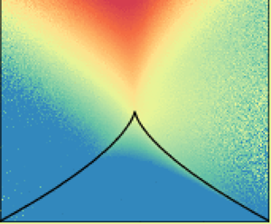This symmetry arises because the rotation rate of the eigenframe about the vorticity axis is a redundant degree of freedom as far as the dynamical evolution of $\lambda _i$ and $\widetilde {\omega }_i$ is concerned. In figure 1 we provide a schematic to illustrate the symmetry transformation.

Figure 1. Schematic to illustrate the symmetry transformation. At any point along a fluid particle trajectory $\boldsymbol {x}(t)$ (or equivalently, at any fixed point in space), the rotation rate of the strain-rate eigenframe (formed by the blue lines) may be modified by adding an arbitrary rotation about the vorticity axis (red line), without affecting the dynamical evolution of either the eigenvalues $\lambda _i$ or the vorticity components in the eigenframe $\widetilde {\omega }_i$.

Before proceeding further, it is worth mentioning how the dynamical symmetry just introduced also relates to the dynamics of other invariants of the velocity gradient $\boldsymbol{\mathsf{A}}$. As discussed in Meneveau (Reference Meneveau2011), for an incompressible flow, $\boldsymbol{\mathsf{A}}$ may be described in terms of the three strain-rate eigenvectors $\boldsymbol {v}_1,\boldsymbol {v}_2,\boldsymbol {v}_3$ and five invariant quantities (Cantwell Reference Cantwell1992)

(2.18a–e)\begin{align} \mathcal{Q}&\equiv-{\textit{A}}_{ij}{\textit{A}}_{ji}/2, \quad\,\, \mathcal{R} \equiv-{\textit{A}}_{ij}{\textit{A}}_{jk}{\textit{A}}_{ki}/3,\nonumber\\ \mathcal{Q}_{S}&\equiv-{\textit{S}}_{ij}{\textit{S}}_{ij}/2, \quad \mathcal{R}_{S}\equiv-{\textit{S}}_{ij}{\textit{S}}_{jk}{\textit{S}}_{ki}/3, \quad \mathcal{V}^2\equiv \omega_i {\textit{S}}_{ij}{\textit{S}}_{jk}\omega_k. \end{align}

These five invariants can be written in terms of $\lambda _i$ and $\widetilde {\omega }_i$ (which are five independent quantities due to incompressibility), e.g.

(2.19a,b)\begin{equation} \mathcal{Q} = -\sum_i\lambda_i^2/2+\sum_i\widetilde{\omega}_i^2/4, \quad \mathcal{R} = -\sum_i\lambda_i^3/3-\sum_i\lambda_i\widetilde{\omega}_i^2/4. \end{equation}

Therefore the symmetry transformation for $\lambda _i$ and $\widetilde {\omega }_i$ also implies the same symmetry transformation for $\mathcal {Q}, \mathcal {R},\mathcal {Q}_{S},\mathcal {R}_{S},\mathcal {V}^2$. That is, the dynamical evolution of the set of invariants $\mathcal {Q}, \mathcal {R},\mathcal {Q}_{S},\mathcal {R}_{S},\mathcal {V}^2$ is unaffected by the transformation $\boldsymbol{\mathsf{W}} \to \boldsymbol{\mathsf{W}} + \gamma \boldsymbol{\mathsf{R}}$.

It is important to note that, while the dynamical evolution of the single-time/single-point invariants $\mathcal {Q}, \mathcal {R},\mathcal {Q}_{S},\mathcal {R}_{S},\mathcal {V}^2$ is not affected by the symmetry transformation (2.12), multi-time/multi-point invariants are in general affected. For example, the invariant $\text {Tr}(\boldsymbol{\mathsf{S}}(\boldsymbol {x},t)\boldsymbol {\cdot } \boldsymbol{\mathsf{S}}(\boldsymbol {x}',t'))$ is affected by the transformation (2.12) since in general the transformation arbitrarily modifies the relative orientations of the eigenframes of $\boldsymbol{\mathsf{S}}(\boldsymbol {x},t)$ and $\boldsymbol{\mathsf{S}}(\boldsymbol {x}',t')$. Nevertheless, the dynamical evolution of multi-time or multi-point products of $\lambda _i,\widetilde {\omega }_i$ is not affected by the symmetry transformation. Multi-time statistics are relevant in a number of fundamental research areas, for example in the framework of Lagrangian refined similarity hypothesis (Yu & Meneveau Reference Yu and Meneveau2010) or Lagrangian chaos (Johnson & Meneveau Reference Johnson and Meneveau2015), and also in applied research areas, as for sub-Kolmogorov droplet deformation (Biferale, Meneveau & Verzicco Reference Biferale, Meneveau and Verzicco2014) and rod/disk spinning and tumbling (Chevillard & Meneveau Reference Chevillard and Meneveau2013). In those contexts, it is important for models to reproduce multi-time statistics. The new symmetry presented in this work may preserve some multi-time statistics for appropriate choices of the multiplier $\gamma$ since that additional degree of freedom may be fixed in the most convenient way, based on the field of application. In which way, and to what extent, the presented symmetry carries over to situations in which multi-time statistics are important deserves further investigation, but it is left for future work. In this paper we focus on single-point and single-time quantities.

2.3. Symmetry transformation for the anisotropic pressure Hessian

The anisotropic/non-local pressure Hessian is defined as

(2.20)\begin{equation} \boldsymbol{\mathcal{H}}\equiv\boldsymbol{\mathsf{H}} - \text{Tr}(\boldsymbol{\mathsf{H}}) \frac{\boldsymbol{\mathsf{I}}}{3}, \end{equation}

which satisfies $\text {Tr}({\boldsymbol{\mathcal{H}}})=0$, and contains all of the non-local part of $\boldsymbol{\mathsf{H}}$. The property that the dynamical evolution of $\lambda _i$ and $\widetilde {\omega }_i$ is not affected by the transformation (2.12) can be interpreted as a symmetry transformation for ${\boldsymbol{\mathcal{H}}}$. To see this, we note that, under the transformation $\boldsymbol{\mathsf{W}} \to \boldsymbol{\mathsf{W}} + \gamma \boldsymbol{\mathsf{R}}$, the equation for $\boldsymbol{\mathsf{A}}$ becomes

(2.21)\begin{equation} {\rm D}_t\boldsymbol{\mathsf{A}} = -\boldsymbol{\mathsf{A}}\boldsymbol{\cdot}\boldsymbol{\mathsf{A}} - \boldsymbol{\mathsf{H}} - \gamma[\boldsymbol{\mathsf{R}},\boldsymbol{\mathsf{S}}] + \nu \nabla^2 \boldsymbol{\mathsf{A}}. \end{equation}

We may then group together $\gamma [\boldsymbol{\mathsf{R}},\boldsymbol{\mathsf{S}}]$ and ${\boldsymbol{\mathcal{H}}}$ to define a transformed anisotropic pressure Hessian

(2.22)\begin{equation} \boldsymbol{\mathcal{H}}_\gamma \equiv \boldsymbol{\mathcal{H}} + \gamma [\boldsymbol{\mathsf{R}},\boldsymbol{\mathsf{S}}]. \end{equation}

The crucial point is that introducing the transformation ${\boldsymbol{\mathcal{H}}}\to {\boldsymbol{\mathcal{H}}}_\gamma$ corresponds to introducing the transformation $\boldsymbol{\mathsf{W}} \to \boldsymbol{\mathsf{W}} + \gamma \boldsymbol{\mathsf{R}}$ into the velocity gradient dynamics, which leaves the dynamical evolution of $\lambda _i$ and $\widetilde {\omega }_i$ unchanged. The additional term $[\boldsymbol{\mathsf{R}},\boldsymbol{\mathsf{S}}]$ in (2.22) is symmetric and traceless, such that ${\boldsymbol{\mathcal{H}}}_\gamma$ preserves the properties of the original anisotropic pressure Hessian ${\boldsymbol{\mathcal{H}}}$. Moreover, the symmetry transformation (2.22) holds for all real and finite values of $\gamma (\boldsymbol {x},t)$, which at this stage is still undetermined.

It is interesting to note that the commutator between the anti-symmetric and symmetric parts of the velocity gradient $[\boldsymbol{\mathsf{R}},\boldsymbol{\mathsf{S}}]$ also arises in the expression for the pressure Hessian obtained in closure models assuming a random velocity field with Gaussian statistics (Wilczek & Meneveau Reference Wilczek and Meneveau2014). In the framework of the Gaussian closure, the coefficient of $[\boldsymbol{\mathsf{R}},\boldsymbol{\mathsf{S}}]$ is the only one that requires specific knowledge of the spatial structure of the flow and must be prescribed by phenomenological closure hypothesis, while all other coefficients of the model can be determined exactly. However, our analysis implies that the ability of the Gaussian closure to predict the dynamics of $\lambda _i$ and $\widetilde {\omega }_i$ will not be impacted by the phenomenological closure hypothesis.

2.4. Using the symmetry transformation for dimensionality reduction

While any finite and real $\gamma$ in (2.22) provides a suitable ${\boldsymbol{\mathcal{H}}}_\gamma$, there may exist certain choices of $\gamma$ that generate configurations of the transformed pressure Hessian ${\boldsymbol{\mathcal{H}}}_\gamma$ that reside on a lower-dimensional manifold in the system, in the sense that some of its eigenvalues are zero. If such configurations exist and are common, this could significantly aid understanding and modelling the complexity of the anisotropic pressure Hessian. To seek for lower-dimensional configurations is equivalent to seeking for configurations in which a rank-reduction on ${\boldsymbol{\mathcal{H}}}_\gamma$ can be performed. We denote the dimensionally reduced form of ${\boldsymbol{\mathcal{H}}}_\gamma$ by ${\boldsymbol{\mathcal{H}}}_\gamma ^*$. Notice that ${\boldsymbol{\mathcal{H}}}_\gamma ^*$ cannot have rank one since $\text {Tr}({\boldsymbol{\mathcal{H}}}_\gamma )=0$, and therefore either $\mathrm {rk}({\boldsymbol{\mathcal{H}}}_\gamma ^*)=2$ or ${\boldsymbol{\mathcal{H}}}_\gamma ^*=\boldsymbol {0}$.

In seeking for lower-dimensional configurations of the anisotropic pressure Hessian, when ${\boldsymbol{\mathcal{H}}}$ is singular (i.e. its rank is less than three and it has at least one zero eigenvalue) the additional term involving $[\boldsymbol{\mathsf{R}},\boldsymbol{\mathsf{S}}]$ in (2.22) is not needed, since ${\boldsymbol{\mathcal{H}}}$ already lives on a lower-dimensional space and we take ${\boldsymbol{\mathcal{H}}}_\gamma ^*={\boldsymbol{\mathcal{H}}}$, which corresponds to $\gamma =0$. On the other hand, when ${\boldsymbol{\mathcal{H}}}$ is not singular we seek for a non-zero vector $\boldsymbol {z}_2$ such that ${\boldsymbol{\mathcal{H}}}_\gamma ^*\boldsymbol {\cdot } \boldsymbol {z}_2=\boldsymbol {0}$, where $\boldsymbol {z}_2$ corresponds to the eigenvector of ${\boldsymbol{\mathcal{H}}}_\gamma ^*$ associated with its zero (and intermediate) eigenvalue. This is equivalent to the generalized eigenvalue problem $\det ({\boldsymbol{\mathcal{H}}}_\gamma ^*)=0$, that is,

(2.23)\begin{equation} \det\left(\boldsymbol{\mathsf{I}} + \gamma\boldsymbol{\mathcal{H}}^{-1}\boldsymbol{\cdot}\left[\boldsymbol{\mathsf{R}},\boldsymbol{\mathsf{S}}\right]\right) = 0. \end{equation}

Notice that ${\boldsymbol{\mathcal{H}}}$ can be safely inverted in (2.23), since the case of singular ${\boldsymbol{\mathcal{H}}}$ has been already taken into account and corresponds to $\gamma =0$. If there exist finite and real values for $\gamma$ that solve (2.23), then those values of $\gamma$ generate a rank-two ${\boldsymbol{\mathcal{H}}}_\gamma ^*$. Defining $\boldsymbol {\mathcal {E}}\equiv {\boldsymbol{\mathcal{H}}}^{-1}\boldsymbol {\cdot }[\boldsymbol{\mathsf{R}},\boldsymbol{\mathsf{S}}]$, the characteristic equation for $\gamma$ is

(2.24)\begin{equation} a\gamma^3 + b\gamma^2 + c\gamma + 1 = 0, \end{equation}

with real coefficients $a,b,c$ given by

(2.25a–c)\begin{equation} a\equiv \det(\boldsymbol{\mathcal{E}}), \quad b\equiv \frac{1}{2}\left(\text{Tr}(\boldsymbol{\mathcal{E}})^2 - \text{Tr}(\boldsymbol{\mathcal{E}\cdot\mathcal{E}})\right), \quad c\equiv \text{Tr}(\boldsymbol{\mathcal{E}}). \end{equation}

The properties of the roots of (2.24) are determined by the discriminant of the polynomial

(2.26)\begin{equation} \varDelta\equiv b^2c^2 - 4ac^3 - 4b^3 - 27a^2 - 18abc. \end{equation}

When $\varDelta =0$, all of the roots of (2.24) are real and at least two are equal, when $\varDelta >0$ there are three distinct real roots, and when $\varDelta <0$ there is one real root and two complex conjugate roots. In every case, provided that $a\neq 0$, there is at least one real root since all the coefficients are real and the degree of the characteristic polynomial is odd. When $a=0$, a real and finite root $\gamma$ may or may not exist according to the value of the discriminant $\varDelta$. This shows that configurations where a rank-two ${\boldsymbol{\mathcal{H}}}_\gamma$ does not exist, that is, the pressure Hessian is intrinsically three-dimensional, may only occur when $a= 0$. Interestingly, $a\equiv \det {\boldsymbol{\mathcal{H}}}^{-1}\det [\boldsymbol{\mathsf{R}},\boldsymbol{\mathsf{S}}]$ (by hypothesis $\det {\boldsymbol{\mathcal{H}}}\ne 0$) and the dimensional reduction of the anisotropic pressure Hessian may not be performed where $\det [\boldsymbol{\mathsf{R}},\boldsymbol{\mathsf{S}}]=0$. The determinant of this commutator can be expressed in terms of the eigenframe variables as

(2.27)\begin{equation} \det[\boldsymbol{\mathsf{R}},\boldsymbol{\mathsf{S}}] = \frac{1}{4}(\lambda_2-\lambda_1)(\lambda_3-\lambda_2)(\lambda_1-\lambda_3) \widetilde{\omega}_1\widetilde{\omega}_2\widetilde{\omega}_3, \end{equation}

so that, when either one or more of the vorticity components in the strain-rate eigenframe is zero, and/or the strain-rate configuration is axisymmetric, a singular ${\boldsymbol{\mathcal{H}}}_\gamma$ may not exist. However, since $\lambda _i$ and $\widetilde {\omega }_i$ have continuous probability distributions, then the probability that $\det [\boldsymbol{\mathsf{R}},\boldsymbol{\mathsf{S}}] =0$ is in fact zero. Therefore, the dimensional reduction of ${\boldsymbol{\mathcal{H}}}_\gamma$ is possible everywhere in the flow except on sets of zero measure.

When (2.24) admits more than one real and finite solution then multiple dimensionally reduced anisotropic pressure Hessians can be defined at the same point, that is, there exist more than a single real and finite multiplier $\gamma$ such that ${\boldsymbol{\mathcal{H}}}_\gamma$ has rank less than three. In this configuration, different ${\boldsymbol{\mathcal{H}}}_\gamma ^*$ can generate the same dynamics of the velocity gradient invariants. We fix this additional degree of freedom by choosing the value of $\gamma$ that provides the maximum alignment between the intermediate eigenvector of the dimensionally reduced anisotropic pressure Hessian and the vorticity. As it will be shown in § 3, this is justified on the basis of the numerical results, which indicate a marked preferential alignment of the intermediate eigenvector of the dimensionally reduced anisotropic pressure Hessian with the vorticity.

The dimensional reduction of the anisotropic pressure Hessian, defined through (2.23), allows for a noticeable reduction of the complexity of the anisotropic pressure Hessian leading to a better understanding of its dynamical effects. Indeed, the fully three-dimensional anisotropic pressure Hessian is specified by five real numbers, being a square matrix of size three. In particular, it takes two numbers to specify the normalized eigenvector $\boldsymbol {y}_1$, one additional number for $\boldsymbol {y}_2$ (then $\boldsymbol {y}_3$ is automatically determined) and two more numbers for the independent eigenvalues $\varphi _1$ and $\varphi _3$ (since $\sum _i\varphi _i=0$). Therefore, the anisotropic pressure Hessian can be expressed in its eigenframe as

(2.28)\begin{equation} \boldsymbol{\mathcal{H}} = \sum_{i=1}^3\varphi_i\boldsymbol{y}_i\boldsymbol{y}_i^{\top}. \end{equation}

We keep the standard convention $\varphi _1\ge \varphi _2\ge \varphi _3$. On the other hand, the dimensionally reduced anisotropic pressure Hessian is specified by only four real numbers. Indeed it is a traceless and singular square matrix of size three. In particular, it takes two numbers to specify the plane orthogonal to the normalized eigenvector $\boldsymbol {z}_2$ an additional number to specify the orientation of $\boldsymbol {z}_1$ on the plane orthogonal to $\boldsymbol {z}_2$ (then $\boldsymbol {z}_3$ is determined) and a number for the single independent eigenvalue $\psi$. Therefore, the dimensionally reduced anisotropic pressure Hessian can be expressed in its eigenframe as

(2.29)\begin{equation} \boldsymbol{\mathcal{H}}_\gamma^* = \psi \left(\boldsymbol{z}_1\boldsymbol{z}_1^{\top} - \boldsymbol{z}_3\boldsymbol{z}_3^{\top}\right), \end{equation}

since the intermediate eigenvector is identically zero and the others satisfy $\psi _1=-\psi _3=\psi$ with $\psi \ge 0$. The pressure Hessian ${\boldsymbol{\mathcal{H}}}_\gamma ^*$ resides locally on the plane $\Pi _2$ orthogonal to $\boldsymbol {z}_2$, which is the tangent space to a more complex manifold. Indeed, the tensor ${\boldsymbol{\mathcal{H}}}_\gamma ^*$ acts on a generic vector $\boldsymbol {q}$ amplifying its component along $\boldsymbol {z}_1$, cancelling its component along $\boldsymbol {z}_2$ and amplifying and flipping its component along $\boldsymbol {z}_3$. The dimensionally reduced anisotropic pressure Hessian is effective only on the plane $\Pi _2$. The eigenvalue of the dimensionally reduced anisotropic pressure Hessian can be related to the full anisotropic pressure Hessian and the vorticity since $\omega _{i}\mathcal {H}_{ij}\omega _j = \omega _{i}\mathcal {H}^*_{\gamma , ij}\omega _j$, which implies

(2.30)\begin{equation} \psi = \frac{ \sum_i\varphi_i (\boldsymbol{y}_i^{\top}\boldsymbol{\cdot\,\omega})^2}{ (\boldsymbol{z}_1^{\top}\,\boldsymbol{\cdot}\,\boldsymbol{\omega})^2- (\boldsymbol{z}_3^{\top}\boldsymbol{\cdot}\,\boldsymbol{\omega})^2}. \end{equation}

Moreover, the tensors ${\boldsymbol{\mathcal{H}}}$ and ${\boldsymbol{\mathcal{H}}}_\gamma ^*$ satisfy the relation $\omega _{i}S_{ij}\mathcal {H}_{jk}\omega _k = \omega _{i}S_{ij}\mathcal {H}^*_{\gamma ,jk}\omega _k$ which yields another equation for the eigenvalue $\psi$:

(2.31)\begin{equation} \psi = \frac{ \sum_i\varphi_i (\boldsymbol{\omega}^{\top}\boldsymbol{\cdot} \boldsymbol{\mathsf{S}}\boldsymbol{\cdot} \boldsymbol{y}_i)(\boldsymbol{y}_i^{\top}\boldsymbol{\cdot}\boldsymbol{\omega})} {(\boldsymbol{\omega}^{\top}\boldsymbol{\cdot} \boldsymbol{\mathsf{S}}\boldsymbol{\cdot} \boldsymbol{z}_1)(\boldsymbol{z}_1^{\top}\boldsymbol{\cdot} \boldsymbol{\omega}) - (\boldsymbol{\omega}^{\top}\boldsymbol{\cdot} \boldsymbol{\mathsf{S}}\boldsymbol{\cdot} \boldsymbol{z}_3)(\boldsymbol{z}_3^{\top}\boldsymbol{\cdot} \boldsymbol{\omega})}. \end{equation}

Equation (2.30) shows that a perfect alignment between $\boldsymbol {z}_2$ and $\boldsymbol {\omega }$ would result in an infinitely large $\psi$, unless the anisotropic pressure Hessian fulfils the condition $\boldsymbol {\omega ^{\top }} \boldsymbol {\cdot } {\boldsymbol{\mathcal{H}}} \boldsymbol {\cdot }\boldsymbol {\omega }=0$. For example, such a peculiar configuration occurs when the flow is exactly two-dimensional, for which ${\boldsymbol{\mathcal{H}}}_\gamma ^*={\boldsymbol{\mathcal{H}}}$. In general, a large eigenvalue $\psi$ corresponds to strong alignment between $\boldsymbol {z}_2$ and $\boldsymbol {\omega }$, as will be discussed in § 3.

This dimensionality reduction brings two-dimensional features into three-dimensional flows, and it is interesting to note that the equations for the velocity gradient already contain another two-dimensional flow feature. In particular, the term $(\omega ^2 - \widetilde {\omega }_i^2)/4$ in (2.10b) arises from the eigenframe representation of $\boldsymbol{\mathsf{R}}\boldsymbol {\cdot } \boldsymbol{\mathsf{R}}=-\omega ^2\boldsymbol{\mathsf{P}}_{\boldsymbol {\omega }}/4$, where $\boldsymbol{\mathsf{P}}_{\boldsymbol {\omega }}$ is the projection tensor on the plane $\Pi _{\boldsymbol {\omega }}$ orthogonal to the vorticity vector $\boldsymbol {\omega }$. This term describes the straining motion in the plane orthogonal to $\boldsymbol {\omega }$ that is associated with the centrifugal force produced by the spinning of the fluid particle about its vorticity axis. As we will discuss later, this two-dimensional effect can be compared with the two-dimensional effect of ${\boldsymbol{\mathcal{H}}}_\gamma ^*$ on the velocity gradient evolution, leading to interesting insights into their respective dynamical roles. Moreover, ${\boldsymbol{\mathcal{H}}}_\gamma ^*$ is a two-dimensional object in a three-dimensional space which opens the possibility to effectively compare pressure Hessian statistics between two-dimensional and three-dimensional flows. However, the tangent space to the manifold defined by ${\boldsymbol{\mathcal{H}}}_\gamma ^*$ varies in space and time, therefore the flow on $\Pi _2$ cannot be directly compared with Euclidean two-dimensional turbulence but with flows in more complex geometries (Falkovich & Gawȩdzki Reference Falkovich and Gawȩdzki2014).

Using the dynamical equivalence of $\boldsymbol {\mathcal {H}}$ and $\boldsymbol {\mathcal {H}}_\gamma ^*$, we may re-write the equation governing $\lambda _i$ (2.10b) as (ignoring the viscous term)

(2.32)\begin{equation} {\rm D}_t{\lambda_{i}} = -\left(\lambda^2_{i}-\frac{1}{3}\sum_j\lambda_j^2\right) - \frac{1}{4}\left( \widetilde{\omega}_i^2 - \frac{1}{3}\sum_j\widetilde{\omega}_j^2\right) -\widetilde{\mathcal{H}}^*_{\gamma,i(i)}, \end{equation}

and in figure 2 we provide a schematic to illustrate the role of each of the terms on the right-hand side of (2.32).

Figure 2. Schematic representation of contribution of the terms on the right-hand side of (2.32). $(a)$ Strain-rate term $-[\boldsymbol{\mathsf{S}} \boldsymbol {\cdot } \boldsymbol{\mathsf{S}} - \text {Tr}(\boldsymbol{\mathsf{S}} \boldsymbol {\cdot } \boldsymbol{\mathsf{S}})\boldsymbol{\mathsf{I}}/3]$ for the typical configuration $\lambda _1 =\lambda _2=-\lambda _3/2$. $(b)$ Rotation term $-[\boldsymbol{\mathsf{R}} \boldsymbol {\cdot }\boldsymbol{\mathsf{R}} - \text {Tr}(\boldsymbol{\mathsf{R}} \boldsymbol {\cdot } \boldsymbol{\mathsf{R}})\boldsymbol{\mathsf{I}}/3]$ which isotropically produces stretching rate along the plane orthogonal to $\boldsymbol {\omega }$ and a compression parallel to $\boldsymbol {\omega }$. $(c)$ Dimensionally reduced anisotropic pressure Hessian $-{\boldsymbol{\mathcal{H}}}_\gamma ^*$ which stretches the fluid element along the $\boldsymbol {z}_3$ direction and compresses it along the $\boldsymbol {z}_1$ direction. $(d)$ Typical configuration for the relative orientation of strain-rate eigenframe, vorticity and dimensionally reduced anisotropic pressure Hessian eigenframe.

3.1. Pressure Hessian dimensional reduction

We first consider the properties of real and finite multipliers $\gamma$, as determined by the numerical solution of (2.24). At each grid point we solve the generalized eigenvalue problem (2.23) to determine real and finite multipliers $\gamma$ for which ${\boldsymbol{\mathcal{H}}}_\gamma ^*$ is singular. In particular, the LAPACK dggev subroutine (Anderson et al. Reference Anderson, Bai, Bischof, Blackford, Demmel, Dongarra, Du Croz, Greenbaum, Hammarling and McKenney1999) has been used to solve the characteristic equation (2.24). The roots of the characteristic equation are in general complex numbers $\widetilde {\gamma } = (\alpha _R + \sqrt {-1}\alpha _I)/\beta$, where $\alpha _R$, $\alpha _I$ and $\beta$ are real numbers. The numerical solution of (2.24) is ill-conditioned when $\det {{\boldsymbol{\mathcal{H}}}}^{-1}\det [\boldsymbol{\mathsf{R}},\boldsymbol{\mathsf{S}}]$ is very small and the division by $\beta$ should be performed carefully. Therefore, at each grid point we first check that $|\beta |>T_1$ (threshold $T_1=10^{-6}$ has been used for the present results) and then we check that $|\alpha _I/\alpha _R| < T_2$ (threshold $T_2=10^{-10}$ has been employed). The tolerance thresholds $T_i$ are absolute numbers since $\gamma$ is non-dimensional. We confirmed that the results are only weakly sensitive to these small tolerance values and we monitored that $\det {\boldsymbol{\mathcal{H}}}_{\gamma }^*$ is actually zero up to the numerical roundoff error.

Figure 3 shows the probability of the multiplicity of real and finite values of $\gamma$ obtained by solving (2.24). All the statistics have been computed by averaging the flow over space and time, a total of ten snapshots spanning six eddy turnover times have been used. The dimensionally reduced anisotropic pressure Hessian exists at the vast majority of the grid points, the configurations with no real and finite multipliers is observed at only about $0.1\,\%$ of the grid points and corresponds to very small values of $\det {\boldsymbol{\mathcal{H}}}^{-1}\det [\boldsymbol{\mathsf{R}},\boldsymbol{\mathsf{S}}]$ in the numerical simulation. The most common case (${\sim }60\,\%$ of the data) corresponds to three real multipliers $\gamma$, that is, three dynamically equivalent pressure Hessians which generate the same dynamics of the velocity gradient invariants. The next most common case (${\sim }40\,\%$ of the data) is a single real root $\gamma$ and a single rank-two ${\boldsymbol{\mathcal{H}}}_\gamma ^*$. The case with two real and finite roots (and the third root asymptotically small compared with these) is rare (${\sim }0.15\,\%$ of the data) and corresponds to $\det [\boldsymbol{\mathsf{R}},\boldsymbol{\mathsf{S}}]$ close to zero. In theconfigurations in which there exist multiple values of $\gamma$, the multiplier which gives the highest alignment between the vorticity vector and the intermediate eigenvector of the dimensionally reduced anisotropic pressure Hessian is selected. Indeed, that preferential alignment is a clear feature of the dimensionally reduced anisotropic pressure Hessian, as we will see below.

Figure 3. Probability of multiplicity of real and finite roots of (2.24).

In figure 4 we show a two-dimensional snapshot of the multiplier field $\gamma (\boldsymbol {x},t)$ for which ${\boldsymbol{\mathcal{H}}}_\gamma$ has rank two, for both the DNS and the surrogate field. As expected, the field $\gamma (\boldsymbol {x},t)$ exhibits a much greater spatial structure in the DNS as compared with the surrogate field, showing how the dimensionality reduction of the anisotropic pressure Hessian depends upon the local structure of the flow. Indeed, since $\gamma (\boldsymbol {x},t)$ is obtained through the solution of (2.24), the spatial variation of $\gamma (\boldsymbol {x},t)$ will reflect the spatial variation of the coefficients of its polynomial equation, and these coefficients depend upon the velocity gradient field.

Figure 4. Two-dimensional snapshot of the multiplier field $\gamma (\boldsymbol {x},t)$ for $(a)$ the actual DNS field and $(b)$ for the surrogate Gaussian field. Colours correspond to the values of $\gamma (\boldsymbol {x},t)$.

The probability density function (PDF) of the multiplier $\gamma$ for which ${\boldsymbol{\mathcal{H}}}_\gamma$ has rank two is shown in figure 5(a). The PDF of $\gamma$ is highly non-Gaussian and $\gamma$ can be very large, even if with a small probability. This may be due to the intermittency of the velocity gradient field, however, since $\gamma$ is obtained from a polynomial equation that depends nonlinearly on the velocity gradients, this nonlinear dependence may also be a cause of the observed non-Gaussianity. As shown in the Appendix, the PDF of $\gamma$ is also non-Gaussian even for the surrogate field; however, the non-Gaussianity is much weaker than in the DNS. Therefore, a substantial source of the non-Gaussianity observed for the PDF of $\gamma$ in the DNS does indeed arise for the dynamical intermittency in the velocity gradients. Another possible source of the strong non-Gaussianity of $\gamma$ would be the high probability of small values of $\det [\boldsymbol{\mathsf{R}},\boldsymbol{\mathsf{S}}]$. In such a case, the matrix used for the reduction, $[\boldsymbol{\mathsf{R}},\boldsymbol{\mathsf{S}}]$, would span the whole three-dimensional domain but with a very small eigenvalue in a certain eigendirection. As a consequence, in order to perform the dimensionality reduction on ${\boldsymbol{\mathcal{H}}}_\gamma \equiv {\boldsymbol{\mathcal{H}}} + \gamma [\boldsymbol{\mathsf{R}},\boldsymbol{\mathsf{S}}]$, the multiplier $\gamma$ must be large enough so that $\gamma [\boldsymbol{\mathsf{R}},\boldsymbol{\mathsf{S}}]$ can compensate the component of ${\boldsymbol{\mathcal{H}}}$ in that eigendirection, and that component may be large. The PDF of $\det [\boldsymbol{\mathsf{R}},\boldsymbol{\mathsf{S}}]$ is shown in figure 5(b). The results show that $\det [\boldsymbol{\mathsf{R}},\boldsymbol{\mathsf{S}}]$ is highly intermittent, being small throughout the vast majority of the flow, but exhibiting extreme fluctuations in very small regions. Indeed, $\det [\boldsymbol{\mathsf{R}},\boldsymbol{\mathsf{S}}]$ is a sixth-order moment of the velocity gradient field. Moreover, the tendency for small values of $\det [\boldsymbol{\mathsf{R}},\boldsymbol{\mathsf{S}}]$ can also be understood in terms of the well-known fact that $\boldsymbol {\omega }$ tends to misalign with $\boldsymbol {v}_3$ (Meneveau Reference Meneveau2011), leading to small values for $\widetilde {\omega }_3$ and therefore to small values of $\det [\boldsymbol{\mathsf{R}},\boldsymbol{\mathsf{S}} ]$ via (2.27). Both of these explanations are supported by the fact that, as shown in the Appendix, the PDF for $\det [\boldsymbol{\mathsf{R}},\boldsymbol{\mathsf{S}}]$ obtained from the surrogate field is almost Gaussian, and there is no preferential alignment of $\boldsymbol {\omega }$ with $\boldsymbol {v}_3$ in the surrogate field.

Figure 5. $(a)$ Probability density function of the real multiplier $\gamma$. $(b)$ The PDF of the determinant of the commutator of anti-symmetric and symmetric part of the velocity gradient, $\det [\boldsymbol{\mathsf{R}},\boldsymbol{\mathsf{S}}]$, the blue curve refers to the blue labels and represents the same PDF over a smaller range. $(c)$ Strain-rate magnitude $\|\boldsymbol{\mathsf{S}}\|^2$ and rotation magnitude $\|\boldsymbol{\mathsf{R}}\|^2$ conditioned on $\det [\boldsymbol{\mathsf{R}},\boldsymbol{\mathsf{S}}]$, the same plot in logarithmic scale is in the inset. $(d)$ Second invariant of the velocity gradient tensor $\mathcal {Q}$ conditioned on $\det [\boldsymbol{\mathsf{R}},\boldsymbol{\mathsf{S}}]$.

We now turn to investigate flow features conditioned on $\det [\boldsymbol{\mathsf{R}},\boldsymbol{\mathsf{S}} ]$. The high probability of observing small values of $\det [\boldsymbol{\mathsf{R}},\boldsymbol{\mathsf{S}} ]$ is consistent with the average of the strain rate and rotation magnitude conditioned on the local value of $\det [\boldsymbol{\mathsf{R}},\boldsymbol{\mathsf{S}} ]$, the results for which are shown in figure 5(c). The values of $\tau _\eta ^2\|\boldsymbol{\mathsf{S}}\|^2$ and $\tau _\eta ^2\|\boldsymbol{\mathsf{R}}\|^2$ when $\det [\boldsymbol{\mathsf{R}},\boldsymbol{\mathsf{S}}]\to 0$, where $\tau _\eta$ is the Kolmogorov time scale, are both slightly less than $1/2$, where $1/2$ is the precise value of the unconditioned averages $\tau _\eta ^2\langle \|\boldsymbol{\mathsf{S}}\|^2\rangle =\tau _\eta ^2\langle \|\boldsymbol{\mathsf{R}}\|^2\rangle$ in isotropic turbulence. For larger values of $\det [\boldsymbol{\mathsf{R}},\boldsymbol{\mathsf{S}} ]$, $\|\boldsymbol{\mathsf{R}}\|^2$ has a well-defined power law scaling, $\|\boldsymbol{\mathsf{R}}\|^2\sim |\det [\boldsymbol{\mathsf{R}},\boldsymbol{\mathsf{S}}]|^{1/3}$, as shown in the inset of figure 5(c). The power law exponent $1/3$ is consistent with simple dimensional analysis. On the other hand, while $\|\boldsymbol{\mathsf{S}}\|^2$ also depends on $\det [\boldsymbol{\mathsf{R}},\boldsymbol{\mathsf{S}}]$ as a power law, the exponent is less than $1/3$, and cannot be predicted by simple dimensional analysis. This is somewhat reminiscent of the results in Buaria et al. (Reference Buaria, Pumir, Bodenschatz and Yeung2019) for $\langle \|\boldsymbol{\mathsf{R}}\|^2\vert \|\boldsymbol{\mathsf{S}}\|^2\rangle$ and $\langle \|\boldsymbol{\mathsf{S}}\|^2\vert \|\boldsymbol{\mathsf{R}}\|^2\rangle$, where they found that the former was well described by dimensional analysis (i.e. by Kolmogorov's 1941 theory, see Pope Reference Pope2000), while the latter was not. The average of the second invariant of the velocity gradient tensor $\mathcal {Q}$ conditioned on the local value of $\det [\boldsymbol{\mathsf{R}},\boldsymbol{\mathsf{S}}]$ is shown in figure 5$(d)$. Interestingly, the region where $\det [\boldsymbol{\mathsf{R}},\boldsymbol{\mathsf{S}}]$ is small is slightly strain-rate dominated (i.e. $\mathcal {Q}<0$). On the other hand, in the regions where $|\det [\boldsymbol{\mathsf{R}},\boldsymbol{\mathsf{S}}]|$ is relatively large, the dynamics is clearly rotation-dominated (i.e. $\mathcal {Q}>0$). When the conditioned average of $\mathcal {Q}$ is weighted with the PDF of $\det [\boldsymbol{\mathsf{R}},\boldsymbol{\mathsf{S}}]$ and integrated over all $\det [\boldsymbol{\mathsf{R}},\boldsymbol{\mathsf{S}}]$ it yields $\left \langle \mathcal {Q} \right \rangle =0$ for isotropic turbulence, which indicates the very large relative weight of regions of the flow contributing to $\langle \mathcal {Q}\vert \det [\boldsymbol{\mathsf{R}},\boldsymbol{\mathsf{S}}]\rangle$ being negative and very small.

3.2. Dimensionally reduced anisotropic pressure Hessian eigenvalue

Figures 6(a) and 6(b) show that, whereas ${\boldsymbol{\mathcal{H}}}$ is in general a fully three-dimensional object with three non-zero eigenvalues $\varphi _i$ that satisfy $\sum _{i=1}^3\varphi _i=0$, ${\boldsymbol{\mathcal{H}}}_\gamma ^*$ is a two-dimensional object with only two active eigenvalues that satisfy $\psi _1=-\psi _3=\psi$, the intermediate eigenvalue being by construction identically zero, $\psi _2=0$. Note that here and throughout, all eigenvectors are unitary, and are ordered so that $\varphi _1 \ge \varphi _2 \ge \varphi _3$. The PDFs of the eigenvalues $\varphi _1\ge 0$ and $\varphi _3\le 0$ of the anisotropic pressure Hessian display marked tails and are almost symmetric with respect to each other. On the contrary, the PDF of $\varphi _2$ has moderate tails and it is positively skewed. The eigenvalue of the dimensionally reduced anisotropic pressure Hessian, $\psi$, exhibits very large fluctuations. Its PDF has wide tails which show that $\psi$, even if with small probability, can take extremely large values. This is in part due to the large intermittency of the flow, giving rise to large values of $[\boldsymbol{\mathsf{R}},\boldsymbol{\mathsf{S}}]$ and $\gamma$ (although with small probability). The large values observed for $\psi$ are also closely related to the statistical geometry in the system. Indeed, the denominator in (2.30) can be very small because, as it will be shown in the next section, the vorticity tends to strongly align with $\boldsymbol {z}_2$, inducing large values of $\psi$. Therefore, the geometrical simplification obtained by replacing the three-dimensional ${\boldsymbol{\mathcal{H}}}$ with the two-dimensional ${\boldsymbol{\mathcal{H}}}_\gamma ^*$ also comes with the cost that the eigenvalue of ${\boldsymbol{\mathcal{H}}}_\gamma ^*$ is far more intermittent than those of ${\boldsymbol{\mathcal{H}}}$.

Figure 6. Probability density function of the eigenvalues of $(a)$${\boldsymbol{\mathcal{H}}}$ and $(b)$ eigenvalues of ${\boldsymbol{\mathcal{H}}}_\gamma ^*$, normalized with the Kolmogorov time scale $\tau _\eta$. $(c)$ Magnitude of the anisotropic pressure Hessian eigenvalues $\varphi =\sqrt {\sum _i\varphi _i^2}$ and anisotropic pressure Hessian eigenvalue, $\psi$, conditioned on the local strain-rate magnitude and $(d)$ on the rotation-rate magnitude.

Next, we condition the eigenvalues of ${\boldsymbol{\mathcal{H}}}$ and ${\boldsymbol{\mathcal{H}}}_\gamma ^*$ on the magnitude of the local strain rate and vorticity $\|\boldsymbol{\mathsf{S}}\|^2$ and $\|\boldsymbol{\mathsf{R}}\|^2$. For the anisotropic pressure Hessian we define $\varphi = \sqrt {\sum _i\varphi _i^2}$ and compute the conditional averages $\left \langle \varphi | \|\boldsymbol{\mathsf{S}}\|^2 \right \rangle$ and $\left \langle \varphi \vert \|\boldsymbol{\mathsf{R}}\|^2 \right \rangle$. Similarly, for the dimensionally reduced anisotropic pressure Hessian we look at $\left \langle \psi \vert \|\boldsymbol{\mathsf{S}}\|^2 \right \rangle$ and $\left \langle \psi \vert \|\boldsymbol{\mathsf{R}}\|^2 \right \rangle$. The results from the DNS are shown in figures 6(c) and 6(d). The results reveal a simple scaling $\left \langle \varphi \vert \|\boldsymbol{\mathsf{S}}\|^2 \right \rangle \sim \|\boldsymbol{\mathsf{S}}\|^2$, as dimensional analysis suggests. This lends support to models such as Wilczek & Meneveau (Reference Wilczek and Meneveau2014), in which the pressure Hessian is a linear combination of $\boldsymbol{\mathsf{S}}^2$, $\boldsymbol{\mathsf{R}}^2$ and $[\boldsymbol{\mathsf{R}},\boldsymbol{\mathsf{S}}]$. The scaling $\left \langle \varphi \vert \|\boldsymbol{\mathsf{S}}\|^2 \right \rangle \sim \|\boldsymbol{\mathsf{S}}\|^2$ is evident especially for large values of $\|\boldsymbol{\mathsf{S}}\|^2$. This may reflect the idea that during large fluctuations, the length scale associated with $\boldsymbol{\mathsf{S}}$ is smaller as compared to situations where $\boldsymbol{\mathsf{S}}$ is small or moderate. If true, then the pressure Hessian is more localized during large fluctuations, giving rise to the scaling $\left \langle \varphi \vert \|\boldsymbol{\mathsf{S}}\|^2 \right \rangle \sim \|\boldsymbol{\mathsf{S}}\|^2$ that reflects a local relationship between $\varphi$ and $\|\boldsymbol{\mathsf{S}}\|^2$. On the other hand, for the dimensionally reduced anisotropic pressure Hessian eigenvalue we find $\left \langle \psi \vert \|\boldsymbol{\mathsf{S}}\|^2 \right \rangle \sim \|\boldsymbol{\mathsf{S}}\|^{2\zeta }$ with $\zeta >1$ (in particular $\zeta$ between $4/3$ and $5/4$). Nevertheless, $\left \langle \psi \vert \|\boldsymbol{\mathsf{S}}\|^2 \right \rangle$ maintains a well-defined power law trend, which has positive implications for modelling the anisotropic pressure Hessian using information inferred by the dimensionally reduced anisotropic pressure Hessian. Moreover, the scalings of the conditioned eigenvalue magnitudes are the same whether conditioned on either $\|\boldsymbol{\mathsf{S}}\|^2$ or $\|\boldsymbol{\mathsf{R}}\|^2$, for both ${\boldsymbol{\mathcal{H}}}$ and ${\boldsymbol{\mathcal{H}}}_\gamma ^*$.

In figure 7 we plot the conditioned averages $\langle \varphi \vert \mathcal {R},\mathcal {Q}\rangle$ and $\langle \psi \vert \mathcal {R},\mathcal {Q}\rangle$. The results show that $\langle \varphi \vert \mathcal {R},\mathcal {Q}\rangle$ is quite large everywhere except for small $\mathcal {R},\mathcal {Q}$ and its shape shares similarities with the sheared drop shape of the joint PDF of the invariants $\mathcal {R},\mathcal {Q}$, that is in figure 12(d). In contrast, $\langle \psi \vert \mathcal {R},\mathcal {Q}\rangle$ is largest in the quadrants $\mathcal {Q}>0,\mathcal {R}<0$ and $\mathcal {Q}<0,\mathcal {R}>0$ (especially below the right Vieillefosse tail) corresponding to regions of enstrophy and strain-rate production. Therefore, it is not only that the magnitudes of $\boldsymbol {\mathcal {H}}$ and ${\boldsymbol{\mathcal{H}}}_\gamma ^*$ differ significantly, but also that they are most active in different regions of the flow. Indeed, ${\boldsymbol{\mathcal{H}}}_\gamma ^*$ is most active in the regions where the velocity gradients are also most active, while $\boldsymbol {\mathcal {H}}$ is active and strong in many regions where the velocity gradients display relatively little activity (e.g. the quadrant $\mathcal {Q}<0$, $\mathcal {R}<0$). In this sense then, one might say that ${\boldsymbol{\mathcal{H}}}_\gamma ^*$ is more closely tied to the dynamics of the velocity gradients than $\boldsymbol {\mathcal {H}}$.

Figure 7. Results for $(a)$$\langle \varphi \vert \mathcal {R},\mathcal {Q}\rangle$, where $\varphi =\sqrt {\sum _i\varphi _i^2}$, and $(b)$$\langle \psi \vert \mathcal {R},\mathcal {Q}\rangle$ as functions of $\mathcal {R},\mathcal {Q}$. Colours denote the magnitude of the terms, and black lines denote the Vieillefosse tails.

5.1. Dimensionally reduced anisotropic pressure Hessian–strain-rate alignment

The components of the dimensionally reduced anisotropic pressure Hessian, ${\boldsymbol{\mathcal{H}}}_\gamma ^*$, in the strain-rate eigenframe can be more conveniently expressed as

(5.1)\begin{equation} \widetilde{\mathcal{H}}_{\gamma,ij}^* = {\textit{V}}_{ki}\mathcal{H}_{\gamma,km}^*{\textit{V}}_{mj} = {\textit{V}}_{ki}{\textit{Z}}_{kp}\Psi_{pq}{\textit{Z}}_{mq}{\textit{V}}_{mj}, \end{equation}

where the matrices $\boldsymbol{\mathsf{V}}$ and $\boldsymbol{\mathsf{Z}}$ contain the components of the strain-rate eigenvectors and dimensionally reduced pressure Hessian eigenvectors in the Cartesian basis, that is, ${\textit{V}}_{ij}\equiv \boldsymbol {e}_i^{\top }\boldsymbol {\cdot }\boldsymbol {v}_j$ and ${\textit{Z}}_{ij}\equiv \boldsymbol {e}_i^{\top }\boldsymbol {\cdot }\boldsymbol {z}_j$. The diagonal and singular matrix $\boldsymbol{\Psi}$ has on its diagonal the eigenvalues of the dimensionally reduced anisotropic pressure Hessian, $(\psi ,0,-\psi )$. The components of ${\boldsymbol{\mathcal{H}}}_\gamma ^*$ in the strain-rate eigenframe (5.1) can be written as

(5.2)\begin{equation} \left[\widetilde{\mathcal{H}}_{\gamma,ij}^*\right] = \psi \begin{bmatrix} \tilde{{z}}_{11}^2 - \tilde{{z}}_{13}^2 & \tilde{{z}}_{11} \tilde{{z}}_{21} - \tilde{{z}}_{13}\tilde{{z}}_{23} & \tilde{{z}}_{11} \tilde{{z}}_{31} - \tilde{{z}}_{13}\tilde{{z}}_{33} \\ \tilde{{z}}_{11} \tilde{{z}}_{21} - \tilde{{z}}_{13}\tilde{{z}}_{23} & \tilde{{z}}_{21}^2 - \tilde{{z}}_{23}^2 & \tilde{{z}}_{21} \tilde{{z}}_{31} - \tilde{{z}}_{23}\tilde{{z}}_{33} \\ \tilde{{z}}_{11} \tilde{{z}}_{31} - \tilde{{z}}_{13}\tilde{{z}}_{33} & \tilde{{z}}_{21} \tilde{{z}}_{31} - \tilde{{z}}_{23}\tilde{{z}}_{33} & \tilde{{z}}_{31}^2 - \tilde{{z}}_{33}^2 \end{bmatrix}, \end{equation}

where $\tilde{z}_{ij}\equiv \boldsymbol {v}_i^{\top }\boldsymbol {\cdot \,z}_j$ is the $i$th strain-rate eigenframe component of the $j$th eigenvector $\boldsymbol {z}_j$ and $\sum _i \tilde{z}_{ij}^2=1$. Since ${\boldsymbol{\mathcal{H}}}_\gamma ^*$ acts only on the plane $\Pi _2$, spanned by $\boldsymbol {z}_1$ and $\boldsymbol {z}_3$, the expression for ${\boldsymbol{\mathcal{H}}}_\gamma ^*$ in the strain-rate eigenframe is much simpler than that for ${\boldsymbol{\mathcal{H}}}$, in that it allows for separation of variables between the magnitude and orientation contributions. The magnitude of ${\boldsymbol{\mathcal{H}}}_\gamma ^*$ is described solely by $\psi$ while the orientation depends on the inner products $\tilde{z}_{ij}$. The factorization into the product of a function only of the eigenvalue and a function only of the alignment of the eigenframes is a feature of two-dimensional traceless tensors, while in three dimensions such separation of variables is in general not possible (Ballouz & Ouellette Reference Ballouz and Ouellette2018).

By introducing the representation (5.2) into (2.32) one obtains

(5.3)\begin{equation} {\rm D}_t{\lambda_{i}} = -\left(\lambda^2_{i}-\frac{1}{3}\sum_j\lambda_j^2\right) - \frac{1}{4}\left( \widetilde{\omega}_i^2 - \frac{1}{3}\sum_j\widetilde{\omega}_j^2\right) + \psi \left(\tilde{{z}}_{i3}^2 - \tilde{{z}}_{i1}^2 \right). \end{equation}

It is known that the blow up of the RE model occurs in the quadrant $\mathcal {R}>0,\mathcal {Q}<0$ where the invariants $\mathcal {R}$ and $\mathcal {Q}$ are defined in (2.18). In particular, the blow-up is associated with the limit $\mathcal {R}\to +\infty$ and $\mathcal {Q}\sim -(27\mathcal {R}^2/4)^{1/3}\to -\infty$ (Vieillefosse Reference Vieillefosse1982). In this quadrant the straining field is in a state of bi-axial extension, with $\lambda _1>0,\lambda _2>0,\lambda _3<0$. Therefore, to explore how ${\boldsymbol{\mathcal{H}}}_\gamma ^*$ prevents blow-up, we must consider its effects on the states where $\lambda _1>0,\lambda _2>0,\lambda _3<0$. From (5.3) we see that the contribution from ${\boldsymbol{\mathcal{H}}}_\gamma ^*$, namely $\psi (\tilde{z}_{i3}^2 - \tilde{z}_{i1}^2)$, will act to prevent blow-up in the quadrant $\mathcal {Q}<0, \mathcal {R}>0$ if $\tilde{z}_{13}^2 - \tilde{z}_{11}^2<0$, $\tilde{z}_{23}^2 - \tilde{z}_{21}^2<0$ and $\tilde{z}_{33}^2 - \tilde{z}_{31}^2>0$.

Figure 10 shows the average alignments between the dimensionally reduced anisotropic pressure Hessian and the strain-rate eigenframe conditioned on the principal invariants of the velocity gradient, $\langle \tilde{z}_{i3}^2 - \tilde{z}_{i1}^2\vert \mathcal {R},\mathcal {Q}\rangle$. The data confirm that, when $\mathcal {Q}<0$ and $\mathcal {R}>0$, $\langle \tilde{z}_{23}^2 - \tilde{z}_{21}^2\vert \mathcal {R},\mathcal {Q}\rangle <0$ and $\langle \tilde{z}_{33}^2 - \tilde{z}_{31}^2\vert \mathcal {R},\mathcal {Q}\rangle >0$, showing that ${\boldsymbol{\mathcal{H}}}_\gamma ^*$ acts to reduce $|\lambda _2|$ and $|\lambda _3|$. However, contrary to expectation, they also show that $\langle \tilde{z}_{13}^2 - \tilde{z}_{11}^2\vert \mathcal {R},\mathcal {Q}\rangle >0$, such that ${\boldsymbol{\mathcal{H}}}_\gamma ^*$ explicitly acts to increase $\lambda _1$ when $\mathcal {Q}<0, \mathcal {R}>0$. Nevertheless, since $\sum _i \lambda _i =0$, if ${\boldsymbol{\mathcal{H}}}_\gamma ^*$ acts to reduce $|\lambda _3|$ when $\mathcal {Q}<0, \mathcal {R}>0$, then it also indirectly acts to reduce $\lambda _1$, since $\lambda _1\to \infty$ is not possible unless $|\lambda _3|\to \infty$ (noting $-\lambda _3\geq \lambda _2$). This indirect effect is mediated via the local pressure Hessian due to the incompressibility constraint. Therefore, the effect of ${\boldsymbol{\mathcal{H}}}_\gamma ^*$ is somewhat subtle, directly acting to prevent blow-up of $\lambda _2$ and $\lambda _3$, and only indirectly acting to prevent the blow-up of $\lambda _1$. Interestingly, the direct amplification of $\lambda _1$ due to ${\boldsymbol{\mathcal{H}}}_\gamma ^*$ becomes very small in a narrow region along the right Vieillefosse tail, as the colours in figure 10(b) show. Therefore, this amplification mechanism is not effective in the phase space region in which the RE system blows up.

Figure 10. Results for $\langle \tilde{z}_{i3}^2 - \tilde{z}_{i1}^2\vert \mathcal {R},\mathcal {Q}\rangle$, $(a)$$i=1$, $(c)$$i=2$, $(e)$$i=3$. The colour range has been truncated to $[-0.3,\ 0.3]$ in order to highlight the trend of the variables around the most probable values. Results for $\langle |\tilde{z}_{i3}^2 - \tilde{z}_{i1}^2|\vert \mathcal {R},\mathcal {Q}\rangle$ in logarithmic scale, $(b)$$i=1$, $(d)$$i=2$, $(\,f)$$i=3$. Black lines denote the Vieillefosse tails.

The scalar products $\tilde{z}_{ij}$ preferentially lie in a very narrow interval around a few well-defined values, as clearly indicated by the results in figure 9. In particular, the eigenvectors $\boldsymbol {z}_{1}$ and $\boldsymbol {z}_{3}$ of ${\boldsymbol{\mathcal{H}}}_\gamma ^*$ tend to form an angle of $(\rm \pi) /4$ with the eigenvectors $\boldsymbol {v}_{1}$ and $\boldsymbol {v}_{3}$ of $\boldsymbol{\mathsf{S}}$. Therefore, a typical configuration for the relative orientation between ${\boldsymbol{\mathcal{H}}}_\gamma ^*$ and $\boldsymbol{\mathsf{S}}$ is

(5.4)\begin{equation} \left[{\textit{V}}_{ki}{\textit{Z}}_{kj}\right] = \begin{bmatrix} \cos\left((\rm \pi)/4+\epsilon_{11}\right) & \sin\left(\epsilon_{12}\right) & \cos\left((\rm \pi)/4+\epsilon_{13}\right)\\ \sin\left(\epsilon_{21}\right) & \cos\left(\epsilon_{22}\right) & \sin\left(\epsilon_{23}\right)\\ \cos\left((\rm \pi)/4+\epsilon_{31}\right) & \sin\left(\epsilon_{32}\right) & \cos\left((\rm \pi)/4+\epsilon_{33}\right) \end{bmatrix}, \end{equation}

where the quantities $\epsilon _{ij}$ represent the deviations of the angles from the idealized configuration considered, and there is a dependence of the sign on the angle between $\boldsymbol {v}_1$ and $\boldsymbol {z}_1$, which can be $(\rm \pi) /4$ or $3(\rm \pi) /4$ (depending upon the chosen sign of the eigenvectors). That sign does not change the discussion below. Considering only small deviations from the most probable alignment, that is, considering $|\epsilon _{ij}|\ll 1$, the elements of the rotation matrix in (5.4) can be Taylor expanded and, at first order in $\epsilon _{ij}$, the expression for the dimensionally reduced anisotropic pressure Hessian in the strain-rate eigenframe (5.2) reduces to

(5.5)\begin{equation} \left[ \widetilde{\mathcal{H}}_{\gamma,ij}^* \right] \sim \psi \begin{bmatrix} -2\epsilon_{11} & \epsilon_{32} & \pm 1 \\ \epsilon_{32} & 0 & \epsilon_{12} \\ \pm 1 & \epsilon_{12} & 2\epsilon_{11} \end{bmatrix}, \end{equation}

where the orthonormality constraint, $\boldsymbol{\mathsf{V}}\boldsymbol {\cdot }\boldsymbol{\mathsf{V}}^{\top }=\boldsymbol{\mathsf{I}}$, has been used to relate the small perturbation angles. It is the diagonal components of ${\boldsymbol{\mathcal{H}}}_\gamma ^*$ that contribute directly to the rate of change of the strain-rate eigenvalues, as in (5.3), and the anisotropic pressure Hessian has no direct effect on the strain-rate eigenvalues when the most probable alignments, $\epsilon _{ij}=0$, occur. At the level of this first-order approximation, the effect of ${\boldsymbol{\mathcal{H}}}_\gamma ^*$ on the first and third eigenvalue always has the opposite sign, which is consistent with the stabilizing effect of the pressure Hessian. Therefore, according to this first-order approximation, the pressure Hessian tends to counteract both $\lambda _1$ and $\lambda _3$ by imposing a negative rate of change of $\lambda _1$ and a positive rate of change of $\lambda _3$, such that both the most positive and negative eigenvalues are pulled toward smaller magnitudes. The results in figure 10 confirm this prediction in the $\mathcal {Q}>0,\mathcal {R}>0$ quadrant, where it is seen that ${{\boldsymbol{\mathcal{H}}}}_\gamma ^*$ acts to suppress the magnitudes of both $\lambda _1$ and $\lambda _3$. That the linearized prediction fails in the region $\mathcal {Q}<0,\mathcal {R}>0$ is perhaps not surprising since that is the region of most intense nonlinear activity, and where ${{\boldsymbol{\mathcal{H}}}}_\gamma ^*$ must be sufficiently large (and by implication $\epsilon _{ij}$ cannot be too small) in order to counteract the blow-up associated with the RE dynamics. The linearization also predicts that the influence of ${\boldsymbol{\mathcal{H}}}_\gamma ^*$ on $\lambda _2$ is only a second-order effect when $\epsilon _{ij}$ is small. However, this prediction is in general not supported by the DNS, since the results in figure 10 show that in most of the $\mathcal {Q},\mathcal {R}$ plane, ${{\boldsymbol{\mathcal{H}}}}_\gamma ^*$ strongly hinders the growth of positive $\lambda _2$.

In order to fully quantify the effect of ${\boldsymbol{\mathcal{H}}}_\gamma ^*$, its magnitude should also be considered together with its orientation. The average of the diagonal components of $-{\boldsymbol{\mathcal{H}}}_\gamma ^*$ in the strain-rate eigenframe conditioned on the invariants $\mathcal {R},\mathcal {Q}$ is shown in figure 11. Despite the large magnitude of the eigenvalue of ${{\boldsymbol{\mathcal{H}}}}_\gamma ^*$, the contribution of ${\boldsymbol{\mathcal{H}}}_\gamma ^*$ to the strain-rate eigenvalue dynamics is moderate on average. Figure 7 shows that the eigenvalue of ${\boldsymbol{\mathcal{H}}}_\gamma ^*$, namely $\psi$, is very large along the right Vieillefosse tail and in the quadrant $\mathcal {Q}>0,\mathcal {R}<0$. Figures 10(a)–10(c) show that $\langle |\tilde{z}_{i3}^2 - \tilde{z}_{i1}^2|\vert \mathcal {R},\mathcal {Q}\rangle$ is small along the right Vieillefosse tail, and these small values of $|\tilde{z}_{i3}-\tilde{z}_{i1}|$ compensate the large magnitude of $\psi$ in the same region. In particular, the orientational contribution of ${\boldsymbol{\mathcal{H}}}_\gamma ^*$ to the dynamics of $\lambda _1$, namely $|\tilde{z}_{13}-\tilde{z}_{11}|$, is very small along the right Vieillefosse tail. This indicates how the direct amplification of $\lambda _1$ due to ${\boldsymbol{\mathcal{H}}}_\gamma ^*$ does not lead to blow up, since this amplification is strong for $\mathcal {R}<0$, but is very weak along the right Vieillefosse tail where RE blows up, as shown in figure 11(a). As observed above, the dimensionally reduced anisotropic pressure Hessian tends to suppress positive values of $\lambda _2$ in the $\mathcal {R}>0,\mathcal {Q}<0$ quadrant, as displayed in figure 11(b). Interestingly, however, ${\boldsymbol{\mathcal{H}}}_\gamma ^*$ contributes to the growth of positive $\lambda _2$ in the region $\mathcal {Q}>0,\mathcal {R}<0$, where $\boldsymbol {\omega }$ and $\boldsymbol {v}_2$ are also strongly aligned (see figure 12b). As such, ${\boldsymbol{\mathcal{H}}}_\gamma ^*$ indirectly contributes to vortex stretching. The results in figure 11(c) show that, the dimensionally reduced anisotropic pressure Hessian strongly hinders $\lambda _3$ along the right Vieillefosse tail, contributing to its amplification only in a small region where $\mathcal {R}<0$ and $\mathcal {Q}>0$. This is a key way in which ${\boldsymbol{\mathcal{H}}}_\gamma ^*$ acts to prevent blow-up in the region $\mathcal {R}>0,\mathcal {Q}<0$.

Figure 11. Results for $\langle -\mathcal {\widetilde {H}}^*_{\gamma ,i(i)}\vert \mathcal {R},\mathcal {Q}\rangle$, the average of the diagonal components of $-{\boldsymbol{\mathcal{H}}}_\gamma ^*$ in the strain-rate eigenframe conditioned on the principal invariants $\mathcal {R},\mathcal {Q}$. $(a)$$i=1$, $(b)$$i=2$, $(c)$$i=3$. Black lines denote the Vieillefosse tails.

5.2. Dimensionally reduced anisotropic pressure Hessian–vorticity alignment

As shown earlier, ${\boldsymbol{\mathcal{H}}}_\gamma ^*$ exhibits remarkable alignment properties with respect to the vorticity $\boldsymbol {\omega }$. In view of this, we now consider how this alignment impacts the way that ${\boldsymbol{\mathcal{H}}}_\gamma ^*$ competes with the centrifugal term produced by vorticity to control the growth of the strain rates. This can be explored by considering the strain rates along the vorticity direction.

The statistical alignments of the vorticity vector with the strain-rate eigenvectors, quantified by $(\boldsymbol {v}_i\ \boldsymbol{\cdot\ \hat {\omega }})^2$, conditioned on the invariants $\mathcal {R}$ and $\mathcal {Q}$, are shown in figure 12. The vorticity tends to align with the most extensional strain-rate eigenvector in the region $\mathcal {R}<0$ and also, to a lesser extent, between the Vieillefosse tails. Alignment between the vorticity and the most compressional strain-rate eigenvector takes place in the region $\mathcal {R}>0$ only, above the right Vieillefosse tail. The vorticity vector strongly aligns with the intermediate strain-rate eigenvector in the region $\mathcal {Q}>0$, close to the $\mathcal {R}=0$ axis and along the right Vieillefosse tail. The half-plane $\mathcal {Q}>0$ and the vicinity of the right Vieillefosse tail correspond to the bulk of probability on the $\mathcal {Q},\mathcal {R}$ plane (Meneveau Reference Meneveau2011), as shown in figure 12(d), and therefore preferential alignment between vorticity and the intermediate strain-rate eigenvector is observed. In the $\mathcal {Q}>0$ region where the alignment between vorticity and the intermediate strain-rate eigenvector is strong, the contribution of ${\boldsymbol{\mathcal{H}}}_\gamma ^*$ to the dynamics of $\lambda _2$ is also strong and positive (see figure 11b). Therefore, ${\boldsymbol{\mathcal{H}}}_\gamma ^*$ plays an important indirect role in the stretching of vorticity by the intermediate eigenvalue in this region.

We now turn to the combined effects of ${\boldsymbol{\mathcal{H}}}_\gamma ^*$ and $\boldsymbol {\omega }$ on the strain-rate dynamics. The evolution equation for $\boldsymbol{\mathsf{S}}$ may be written as (ignoring the viscous term)

(5.6)\begin{equation} {\rm D}_t\boldsymbol{\mathsf{S}}=-\left(\boldsymbol{\mathsf{S}}\boldsymbol{\cdot}\boldsymbol{\mathsf{S}}-\frac{1}{3} \text{Tr}(\boldsymbol{\mathsf{S}}\boldsymbol{\cdot}\boldsymbol{\mathsf{S}}) \boldsymbol{\mathsf{I}} \right) -\frac{1}{4}\left(\boldsymbol{\omega}\boldsymbol{\omega}^{\top}- \frac{1}{3} \omega^2 \boldsymbol{\mathsf{I}} \right)-\boldsymbol{\mathcal{H}}. \end{equation}

When we consider the projection of this equation along the instantaneous vorticity direction $\hat {\boldsymbol {\omega }}\equiv \boldsymbol {\omega }/\omega$, the contribution of the last two terms on the right-hand side of (5.6) is

(5.7)\begin{equation} \hat{\boldsymbol{\omega}}^{\top}\boldsymbol{\cdot} \left(-\frac{1}{4}\boldsymbol{\omega}\boldsymbol{\omega}^{\top}+ \frac{1}{12} \omega^2 \boldsymbol{\mathsf{I}} -\boldsymbol{\mathcal{H}} \right) \boldsymbol{\cdot}\hat{\boldsymbol{\omega}} = -\frac{1}{6}\omega^2 + \psi\left( (\hat{\boldsymbol{\omega}}\boldsymbol{\cdot}\boldsymbol{z}_3)^2 - (\hat{\boldsymbol{\omega}}\boldsymbol{\cdot}\boldsymbol{z}_1)^2\right), \end{equation}

where the properties of ${\boldsymbol{\mathcal{H}}}_{\gamma }^*$ have allowed us to replace ${\boldsymbol{\mathcal{H}}}$ with ${\boldsymbol{\mathcal{H}}}_{\gamma }^*$ on the right-hand side of (5.7). Note that the term $-\omega ^2/6$ comes entirely from the contribution of vorticity to the isotropic part of the pressure Hessian, since the centrifugal contribution does not act along the direction of vorticity, but only in directions orthogonal to it. Equation (5.7) shows that (notice that $\psi \geq 0$) when the vorticity is more aligned with the extensional/compressional direction of ${\boldsymbol{\mathcal{H}}}_\gamma ^*$, then ${\boldsymbol{\mathcal{H}}}_\gamma ^*$ acts with/against the contribution from vorticity to oppose/aid the production of strain rate along the vorticity direction. In figure 13 we consider the DNS data for $\langle (\hat {\boldsymbol {\omega }}\boldsymbol {\cdot }\boldsymbol {z}_3)^2-(\hat {\boldsymbol {\omega }}\boldsymbol {\cdot }\boldsymbol {z}_1)^2 \vert \mathcal {R},\mathcal {Q}\rangle$. The results show that, in $\mathcal {Q}>0$ regions, the vorticity vector preferentially aligns with the most compressional eigenvector of ${\boldsymbol{\mathcal{H}}}_{\gamma }^*$, so that $\langle (\hat {\boldsymbol {\omega }}\boldsymbol {\cdot }\boldsymbol {z}_3)^2-(\hat {\boldsymbol {\omega }}\boldsymbol {\cdot }\boldsymbol {z}_1)^2 \vert \mathcal {R},\mathcal {Q}\rangle >0$. On the contrary, in $\mathcal {Q}<0$ regions $\langle (\hat {\boldsymbol {\omega }}\boldsymbol {\cdot }\boldsymbol {z}_3)^2-(\hat {\boldsymbol {\omega }}\boldsymbol {\cdot }\boldsymbol {z}_1)^2 \vert \mathcal {R},\mathcal {Q}\rangle <0$. This striking behaviour means that in vorticity dominated regions, the dynamical effect of ${\boldsymbol{\mathcal{H}}}_\gamma ^*$ is to increase the strain rate along the vorticity direction, and the opposite in strain-rate-dominated regions.

Figure 12. Results for $\langle (\hat {\boldsymbol {\omega }}\boldsymbol {\cdot }\boldsymbol {v}_i)^2\vert \mathcal {R},\mathcal {Q}\rangle$, the statistical alignment between vorticity and eigenvectors of the strain-rate tensor, conditioned on the principal invariants $\mathcal {R},\mathcal {Q}$. $(a)$$i=1$, $(b)$$i=2$, $(c)$$i=3$. Panel $(d)$ shows the joint probability density of the principal invariants $\mathcal {R}$ and $\mathcal {Q}$. Black lines denote the Vieillefosse tails.

Figure 13. Statistical alignment between vorticity and eigenvectors of the dimensionally reduced anisotropic pressure Hessian, conditioned on the principal invariants $\mathcal {R},\mathcal {Q}$. Results for $(a)$$\langle (\hat {\boldsymbol {\omega }}\boldsymbol {\cdot }\boldsymbol {z}_3)^2-(\hat {\boldsymbol {\omega }}\boldsymbol {\cdot }\boldsymbol {z}_1)^2 \vert \mathcal {R},\mathcal {Q}\rangle$ and $(b)$$\langle |(\hat {\boldsymbol {\omega }}\boldsymbol {\cdot }\boldsymbol {z}_3)^2-(\hat {\boldsymbol {\omega }}\boldsymbol {\cdot }\boldsymbol {z}_1)^2| \vert \mathcal {R},\mathcal {Q}\rangle$ in logarithmic scale. Black lines denote the Vieillefosse tails.