


1. Introduction
Exponential growth of perturbations has been the classical belief of what is happening in turbulence. In the linear hydrodynamic instability theory, exponential growth of perturbations is the main idea for the explanation of transition from laminar to turbulent flow. Recent rigorous mathematical results show that the linear approximation in inviscid hydrodynamic instability theory fails (Li Reference Li2013, Reference Li2018). Thus linear inviscid hydrodynamic instability cannot provide a good approximation for the amplification of perturbations. This suggests that amplification of perturbations in turbulence may be a more complicated matter than previously thought. Indeed, based on rigorous mathematical analysis (Li Reference Li2014, Reference Li2017; Inci Reference Inci2015; Inci & Li Reference Inci and Li2019), we predicted that the growth of perturbations in fully developed turbulence is faster than exponential, and the aim of the current paper is to numerically verify our prediction. With the development of chaos theory, chaos was thought to be what is happening in turbulence (Ruelle & Takens Reference Ruelle and Takens1971). Chaos theory is based on exponential growth of perturbations. Chaos is often in the form of a strange attractor which is characterized by exponential amplifications of perturbations within the attractor, with the coefficient of the exponent being the so-called Lyapunov exponent. On the other hand, fully developed turbulence behaves very differently from low-dimensional chaos, the onset of fully developed turbulence is more abrupt, and fully developed turbulence is more violent than low-dimensional chaos. When viewed in phase spaces, the projection of fully developed turbulence onto low-dimensional subspace does not seem to have the recurrence property of chaos.
Ever since Ruelle and Takens introduced the idea of chaos for understanding the mechanism of turbulence (Ruelle & Takens Reference Ruelle and Takens1971), there has been constant effort in validating the idea (Bohr et al. Reference Bohr, Jensen, Paladin and Vulpiani2005). At moderate Reynolds number, some features of chaos are indeed embedded in transient turbulence (Kawahara & Kida Reference Kawahara and Kida2001; Viswanath Reference Viswanath2007; Gibson, Halcrow & Cvitanović Reference Gibson, Halcrow and Cvitanović2008; van Veen & Kawahara Reference van Veen and Kawahara2011; Kawahara, Uhlmann & van Veen Reference Kawahara, Uhlmann and van Veen2012; Kreilos & Eckhardt Reference Kreilos and Eckhardt2012; Lucas & Kerswell Reference Lucas and Kerswell2015). A key measure of chaos is the Lyapunov exponent. Ruelle predicted that the maximal Lyapunov exponent in homogeneous isotropic turbulence is proportional to the square root of the Reynolds number  $\sigma \sqrt {Re}$ (Ruelle Reference Ruelle1979; Crisanti et al. Reference Crisanti, Jensen, Vulpian and Paladin1993; Aurell et al. Reference Aurell, Boffetta, Crisanti, Paladin and Vulpiani1996, Reference Aurell, Boffetta, Crisanti, Paladin and Vulpiani1997; Boffetta et al. Reference Boffetta, Cencini, Falcioni and Vulpiani2002; Boffetta & Musacchio Reference Boffetta and Musacchio2017; Berera & Ho Reference Berera and Ho2018). Extensive numerical studies on Ruelle's prediction have been conducted over the years (Crisanti et al. Reference Crisanti, Jensen, Vulpian and Paladin1993; Aurell et al. Reference Aurell, Boffetta, Crisanti, Paladin and Vulpiani1996, Reference Aurell, Boffetta, Crisanti, Paladin and Vulpiani1997; Boffetta et al. Reference Boffetta, Cencini, Falcioni and Vulpiani2002; Boffetta & Musacchio Reference Boffetta and Musacchio2017; Berera & Ho Reference Berera and Ho2018). Ruelle's prediction is obtained via dimensional analysis under the assumption that the maximal Lyapunov exponent is the inverse of the Kolmogorov time scale which makes numerical resolution a challenging problem. We predicted that the maximal amplification of perturbations in fully developed turbulence is faster than exponential (Li Reference Li2014, Reference Li2018), and is given by
 \begin{equation} \exp({\sigma \sqrt{Re} \sqrt{t} +\sigma_1 t}) , \end{equation}
where  $\sigma$ and
  $\sigma _1 = \sqrt {({e}/{2})} \sigma$ are two positive constants that are determined by the temporal maximum of the Sobolev norm of the base solution where the perturbations are added to, and the base solution approaches the corresponding solution of Euler equations as
  $Re \rightarrow \infty$ on any finite time interval of existence. As
  $Re \rightarrow \infty$,
  $\sigma$ and
  $\sigma _1$ approach finite positive values. This maximal amplification estimate is rigorously derived as an upper bound on the solutions to the linear Navier–Stokes equations without any assumption (Li Reference Li2014) (see appendix A). The linear Navier–Stokes equations are the governing equations of the linear evolution of the perturbations. We use functional analysis tools to achieve an upper bound on the solutions to the linear Navier–Stokes equations. The
  $\sigma \sqrt {Re} \sqrt {t}$-term in the estimate is a result of the interaction between viscosity and nonlinearity. It is obtained from a Gronwall inequality estimate on the variation of parameters form of the linear Navier–Stokes equations. Unlike in finite dimensions, the maximal growth of perturbations here is the supremum (not maximum) of all growths of perturbations. In finite dimensions, the maximum can be achieved by a specific perturbation. In infinite dimensions, the supremum cannot be achieved by any specific perturbation. But the supremum can be approached by different perturbations, for more details see (Feng & Li Reference Feng and Li2020) where a sequence of perturbations with greater and greater growth can be constructed from two perturbations. On the other hand, as shown below and in Feng & Li (Reference Feng and Li2020), the
  $\sqrt {t}$-nature in the exponent of the estimate is observed for generic perturbations in fully (and non-fully) developed turbulence for various values of the constant
  $\sigma$, and the
  $\sqrt {Re}$-nature in the exponent of the estimate is also observed for generic perturbations in fully developed turbulence for various values of the constant
  $\sigma$. The
  $\sigma _1 t$-term in the exponent of the estimate represents a Lyapunov exponential growth, but unlike Ruelle's assumption, the Lyapunov exponent
  $\sigma _1$ approaches a finite positive value rather than infinity like
  $\sqrt {Re}$ as
  $Re \rightarrow \infty$. When studying the unstable eigenvalues (realizations of
  $\sigma _1$) of steady states in two-dimensional Kolmogorov flow, we indeed found analytically that the unstable eigenvalues approach finite positive values which are the corresponding inviscid unstable eigenvalues (Li Reference Li2005). The
  $\sigma \sqrt {Re} \sqrt {t}$-term in the exponent of the estimate is the newly discovered growth rate. Unlike Ruelle's prediction of
  $\sigma \sqrt {Re} \, t$, it is
  $\sigma \sqrt {Re} \sqrt {t}$. In general, the linear temporal evolution of a perturbation as a solution to the linear Navier–Stokes equations is a function of time. There is no reason that the temporal growth of perturbations has to be exponential in time. Here, we predict that it is exponential in the square root of time. We envision that this square root of time nature corresponds to the abrupt onset and violent nature of fully developed turbulence in contrast to low-dimensional chaos. When the time
  $t$ is small,
  $\sqrt {t}$ is much bigger than
  $t$. Thus we predicted that initial stage maximal amplification of perturbations is superfast (much faster than exponential). Together with the large Reynolds number in the fully developed turbulence regime, such superfast amplification of perturbations will quickly reach nonlinear saturation during which time the second exponent term
  $\sigma _1 t$ is much smaller than the first term
  $\sigma \sqrt {Re} \sqrt {t}$. After the nonlinear saturation, the linear Navier–Stokes equations are no longer a good approximation on the evolution of perturbations, nonlinearity takes over, the size of the perturbations already reaches order one in comparison with the base flow, and the growth estimate (1.1) does not apply anymore, in fact, the perturbations will stay bounded afterwards as discussed in next section on nonlinear amplification of perturbations.
We have conducted an extensive low resolution numerical verification on our prediction (Feng & Li Reference Feng and Li2020). Our low resolution numerical simulations were not able to get into fully developed turbulence regime. On the other hand, that numerical investigation showed that our analytical prediction applies to a wide regime beyond fully developed turbulence. Built upon our earlier numerical verification (Feng & Li Reference Feng and Li2020), here, we conduct a large numerical verification with resolution up to  $2048^3$ and Reynolds number up to
  $6210$. We carry out direct numerical simulations on the three-dimensional Navier–Stokes equations in the homogeneous isotropic turbulence regime. It is in such a fully developed homogeneous isotropic turbulence regime that our analytical prediction is most likely to be accurate. Our numerical results here indeed confirm our analytical prediction. Our numerical simulation also demonstrates that such superfast amplification of perturbations leads to superfast nonlinear saturation. We conclude that such superfast amplification and superfast nonlinear saturation of ever existing perturbations suggest a mechanism for the generation, development and persistence of fully developed turbulence.
Unlike the Lagrangian approach which tracks the trajectories of individual fluid particles, here we use the Eulerian approach which tracks the evolution of the entire fluid field starting from an initial condition of the fluid field. We will add a perturbation to the initial condition and track the evolution of the perturbation either nonlinearly or linearly. By subtracting the two fluid fields, we are tracking the evolution of the perturbation nonlinearly. By subtracting the Navier–Stokes equations along the two fluid fields, we get the governing equations of the nonlinear evolution of the perturbation. By dropping the nonlinear terms of the perturbation, we get the governing equations of the linear evolution of the perturbation, i.e. the linear Navier–Stokes equations and by solving which we track the evolution of the perturbation linearly.
2. The results
We conduct direct numerical simulations on the three-dimensional Navier–Stokes equations under periodic boundary condition of period  $(2{\rm \pi} )^3$ with a de-aliased pseudo-spectral code (Yoffe Reference Yoffe2012)
 \begin{equation} \partial_t \boldsymbol{u} + \boldsymbol{u} \boldsymbol{\cdot} \boldsymbol{\nabla} \boldsymbol{u} = -\boldsymbol{\nabla} p + \nu {\rm \Delta} \boldsymbol{u} +\boldsymbol{f}, \quad \boldsymbol{\nabla} \boldsymbol{\cdot} \boldsymbol{u} = 0, \end{equation}
where  $\boldsymbol {u}$ is the velocity field,
  $p$ is the pressure,
  $\nu$ is the viscosity and
  $\boldsymbol {f}$ is the external forcing. The external forcing will only force low wavenumbers (large scales), and the Fourier transform
  $\tilde {\boldsymbol {f}}$ of
  $\boldsymbol {f}$ is given by Machiels (Reference Machiels1997)
 \begin{align} \tilde{\boldsymbol{f}} (\boldsymbol{k} , t) = \begin{cases} \dfrac{\epsilon_f}{2E_f} \tilde{\boldsymbol{u}} (\boldsymbol{k}, t), & \text{if}\ 0< |\boldsymbol{k} | < k_f ,\\ 0, & \text{otherwise}, \end{cases} \end{align}
where  $\tilde {\boldsymbol {u}} (\boldsymbol {k}, t)$ is the Fourier transform of the velocity field
  $\boldsymbol {u}$,
  $E_f$ is the kinetic energy restricted to the forcing band,
  $E_f = \frac {1}{2} \sum _{0< |\boldsymbol {k} | < k_f} | \tilde {\boldsymbol {u}} (\boldsymbol {k}, t)|^2$, and one can view the external forcing as an energy pumping through the low wavenumbers with the energy pumping rate
  $\epsilon _f$, from the following energy equation
 \begin{equation} \frac{\textrm{d}}{\textrm{d}t} \sum_{\boldsymbol{k}} |\tilde{\boldsymbol{u}}|^2 = -\nu \sum_{\boldsymbol{k}} |\boldsymbol{k} \tilde{\boldsymbol{u}}|^2 + \epsilon_f . \end{equation}
Here, the first term on the right-hand side is the turbulence energy dissipation rate. Through such energy pumping that balances the energy dissipation, one can drive the turbulence into a statistically steady state of homogeneous isotropic turbulence. The external forcing here has been well tested by other researchers (Kaneda & Ishihara Reference Kaneda and Ishihara2006; Linkmann & Morozov Reference Linkmann and Morozov2015). For our numerical simulations here, we choose  $k_f = 2.5$ and
  $\epsilon _f = 0.1$. The Reynolds number is specifically defined by
  $Re = {VL}/{\nu }$, where
  $V$ is the root-mean-square velocity, and
  $L$ is the integral length scale
  $L = ({3{\rm \pi} }/{8E}) \sum _{\boldsymbol {k}} ({| \tilde {\boldsymbol {u}} (\boldsymbol {k} )|^2}/{|\boldsymbol {k} |})$, where
  $E$ is the kinetic energy. The large eddy turnover time is given by
  $T_0 = L/V$. In our simulations, the large eddy turnover time is approximately
  $2$. All our direct numerical simulations are well resolved to scales smaller than the Kolmogorov scale. We also test resolution to scales much smaller than the Kolmogorov scale to make sure our resolution is statistically sufficient.
After we run our direct numerical simulation to a statistically steady state of homogeneous isotropic turbulence, we introduce a perturbation by first making a copy of the velocity field at a time step and then not calling the external forcing at that time step for one copy of the velocity field. Thus the perturbation will be in the band of wavenumbers of the external forcing (2.2),  $0< |\boldsymbol {k} | < k_f$. After that time step, both fields will call the external forcing normally. We can then track the nonlinear or linear evolution of the perturbation as described before. We denote the nonlinear evolution of the perturbation by
  ${\rm \Delta} \boldsymbol {u} (\boldsymbol {x} , t)$, the linear evolution of the perturbation by
  $\delta \boldsymbol {u} (\boldsymbol {x} , t)$ and their energy norms by
  $\varDelta (t) = {\rm \Delta} u (t)$ and
  $\delta (t) =\delta u (t)$
 \begin{gather} \varDelta (t) = {\rm \Delta} u (t) = \left (\sum_{\boldsymbol{k}} |\widetilde{{\rm \Delta} \boldsymbol{u}} (\boldsymbol{k} , t)|^2 \right )^{1/2} , \end{gather}
 \begin{gather}\delta (t) =\delta u (t) = \left (\sum_{\boldsymbol{k}} |\widetilde{\delta \boldsymbol{u}} (\boldsymbol{k} , t)|^2 \right )^{1/2} . \end{gather}
We notice that the nonlinear amplification  ${\rm \Delta} u (t)$ is bounded in time. Under inviscid dynamics, the kinetic energies of both the base solution and the perturbed solution (i.e. base solution plus a perturbation) are conserved, and this leads to the kinetic energy of the perturbation being bounded by the kinetic energy of the base solution and the initial kinetic energy difference between the base solution and the perturbed solution. Since the forcing in the Navier–Stokes equations is balanced by the viscous dissipation in order to maintain a statistically steady state (homogeneous isotropic turbulence), the kinetic energy of the perturbation is still bounded under viscous dynamics (see also the supplementary material of Berera & Ho Reference Berera and Ho2018). On the other hand, the above argument does not apply to the linear evolution of the perturbation, which is governed by the linearized Navier–Stokes equations along the base solution. The linear amplification
  $\delta u (t)$ is unbounded in time. Our prediction (1.1) is for the linear amplification
  $\delta u (t)$. During the early stage (small time) amplification, the linear amplification
  $\delta u (t)$ is a good approximation of the nonlinear amplification
  ${\rm \Delta} u (t)$, and our prediction (1.1) also applies to the nonlinear amplification
  ${\rm \Delta} u (t)$. Then the linear amplification and the nonlinear amplification are going to diverge, that is the transition to nonlinear saturation, and the linear amplification is not a good approximation of the nonlinear amplification anymore. We want to emphasize that the nonlinear amplification is what is happening in reality. We are interested in the initial stage amplification until the nonlinear saturation. Of course, the nonlinear saturation depends on the initial energy norm of the perturbation
  ${\rm \Delta} u (0)$, but it also depends on the Reynolds number. In figure 1, we show the nonlinear saturation for an initial perturbation with the energy norm
  ${\rm \Delta} u (0) = \delta u (0) = 0.01$ and the Reynolds number
  $Re = 230$. Divergence of the linear and nonlinear amplifications happens around
  $t=10$ which is approximately
  $5$ large eddy turnover time
  $5 T_0$, when nonlinear saturation sets in. After the nonlinear saturation, nonlinearity takes over, and the nonlinear evolution of the perturbation stays bounded (its magnitude actually fluctuates around a constant value), while the linear evolution of the perturbation continues amplifying. We also observed that increasing the Reynolds number will drastically reduce the nonlinear saturation time, and increasing the energy norm of the initial perturbation of course will also reduce the nonlinear saturation time. In the exponent of the estimate (1.1), the
  $\sigma \sqrt {Re} \sqrt {t}$ term dominates (is greater than) the
  $\sigma _1 t$ term when
  $t \in [0, (\sigma /\sigma _1)^2 Re ]$. In figure 1, the length of this dominance interval [
 $0, (\sigma /\sigma _1)^2 Re$] is about
  $170$, while the nonlinear saturation sets in at approximately
  $t=10$ (where the ratio of the
  $\sigma _1 t$ term to the
  $\sigma \sqrt {Re} \sqrt {t}$ term is approximately
  $1$ to
  $4$). When we increase
  $Re$, the dominance interval [
 $0, (\sigma /\sigma _1)^2 Re$] increases, but the nonlinear saturation time decreases. Thus before nonlinear saturation, the
  $\sigma _1 t$ term is much smaller than the
  $\sigma \sqrt {Re} \sqrt {t}$ term. So when the Reynolds number is large, we have a superfast nonlinear saturation. Such superfast nonlinear saturation is of course caused by the superfast amplification of the perturbation due to the
  $\sigma \sqrt {Re} \sqrt {t}$ term.

Figure 1. The divergence of the linear amplification and the nonlinear amplification of a perturbation with initial energy norm  ${\rm \Delta} u (0) = \delta u (0) = 0.01$ (2.4) and (2.5) and the Reynolds number
  $Re = 230$. The vertical axis symbol
  $r (t)$ represents either
  ${{\rm \Delta} u (t)}/{{\rm \Delta} u (0)}$ or
  ${\delta u (t)}/{\delta u (0)}$. Divergence and nonlinear saturation happens around
  $t=10$ which is approximately
  $5$ large eddy turnover times
  $5 T_0$. The inset zooms in the time interval
  $t\in [0, 6]$. The dashed line is the fitting curve
  $0.9 \sqrt {t} + 0.34 t$ of the type in the exponent of our estimate (1.1).
In figure 1, we fit the linear amplification with the fitting curve  $0.9 \sqrt {t} + 0.34 t$ which is of the type in the exponent of our estimate (1.1). The fitting curve fits well before
  $t=20$. Around
  $t=20$, the fitting curve diverges from the linear amplification. Notice that the base solution is turbulent, so the solution to the linearized equations can be very complicated in
  $t$ (in short time, it can be approximated by the difference of two turbulent solutions). In principle,
  $\delta u(t)$ can take any shape. Expecting
 \begin{equation} \delta u(t) \sim \delta u(0) \exp({c_1 \sqrt{t} + c_2 t}) \end{equation}
for all time, is unrealistic. Notice also that our estimate is on the maximal amplification of perturbations at any time in fully developed turbulence (see appendix A). If an individual perturbation amplification gets close to the maximal amplification at one time, then at another time it may be far away from the maximal amplification. Once again, expecting an individual perturbation amplification to follow (2.6) for all time is unrealistic.
From now on, we will mainly focus on the time before nonlinear saturation when the linear amplification is a good approximation of the nonlinear amplification of perturbations to verify our prediction (1.1), and all the rest of the numerical simulations are presented with the nonlinear amplifications of perturbations unless specifically noted. Since the initial perturbations are called at somewhat random time steps, the sizes of initial perturbations in all our numerical simulations here are not exactly the same, but they are all approximately  $0.01$.
In figure 2, we show the nonlinear amplifications of perturbations for the Reynolds numbers  $Re = 130, 805, 1450, 2520, 6210$ before their nonlinear saturations so that the linear amplifications are good approximations of the nonlinear amplifications. Our goal is twofold: first verify the
  $\sqrt {t}$-nature in the exponent of our prediction (1.1) for the linear amplifications, and second, to show that, in reality, we can observe this
  $\sqrt {t}$-nature for the nonlinear amplifications before the nonlinear saturations. When
  $Re = 130$, the nonlinear saturation is around
  $t=20$. As the Reynolds number increases, the nonlinear saturation time decreases. When
  $Re = 2520$, the nonlinear saturation is around
  $t=1$, and when
  $Re = 6210$, the nonlinear saturation is around
  $t=0.5$. Except in
  $t \rightarrow 0^+$ limit, we clearly observed the amplifications of
  $\textrm {e}^{c \sqrt {t}}$ in
  $t$ as we predicted in (1.1). We use
  $c$ to represent a generic constant in this paper. Since the
  ${1}/{\sqrt {t}}$ factor is already incorporated into the vertical axis, the horizontal portion of each curve corresponds to the amplification of
  $\textrm {e}^{c \sqrt {t}}$. As the Reynolds number increases, we can see clearly the trend of the curves going horizontal in the plotted time interval. Each curve goes through the same process of superfast amplification and superfast nonlinear saturation as in figure 1. When the Reynolds number is larger, the nonlinear saturation sets in much earlier. As discussed earlier in the Introduction, no specific perturbation can achieve the maximal amplification (1.1), nevertheless here for the perturbations that are somewhat randomly called inside the homogeneous isotropic turbulence, we still observe the
  $\sqrt {t}$-nature in the exponent of the estimate (1.1) even though the constant
  $c$ does not reach the maximal value of
  $\sigma \sqrt {Re}$ in (1.1). The
  $\sqrt {t}$-nature in the exponent turns out to be generic with respect to the perturbations and the base solutions that we numerically tested. We also tested white noise perturbations, and we observe the same
  $\sqrt {t}$-nature. Figure 3 shows a sample of
  $20$ simulations with white noise initial perturbations and their average with an average Reynolds number
  $Re =230$ (see appendix B for a longer time simulation). Our base solutions here are the random ensemble realizations in the homogeneous isotropic turbulence. The
  $\sqrt {t}$-nature does not depend on which realization. In our earlier low resolution numerical simulations (Feng & Li Reference Feng and Li2020), we tested extensively other types of base solutions and perturbations, and we always observed the same
  $\sqrt {t}$-nature, even for non-fully developed turbulence. In the
  $t \rightarrow 0^+$ limit, numerical resolution can never be sufficient and generates false results, as shown by an explicit example in Li (Reference Li2017) and Feng & Li (Reference Feng and Li2020). In Li (Reference Li2017), we found a family of exact solutions, in the Fourier series form, to the unforced two-dimensional Kolmogorov flow. Each of the solutions can be viewed as a base solution. The perturbation that we were able to study is from one solution to another solution, i.e. the perturbation is within the family of solutions. We can calculate explicitly that the fastest amplifying Fourier mode of the perturbation is given by
  $k \sim {1}/{\sqrt {t}}$. As
  $t \rightarrow 0^+$,
  $k \rightarrow \infty$. Thus when
  $t \rightarrow 0^+$, numerical finite Fourier truncations will always miss the fastest amplifying Fourier mode of the perturbation, and produce much lower false growth. In Feng & Li (Reference Feng and Li2020), we carefully verified this. No matter how many Fourier modes were included in the numerical simulations, the numerically calculated growth of the perturbation was always lower than the analytical lower bound of the growth of the perturbation as
  $t \rightarrow 0^+$ – a false result! For turbulence, we surely do not expect numerical simulations can do better than for the simple explicit example.

Figure 2. The nonlinear amplifications of perturbations for different Reynolds numbers  $Re = 130, 805, 1450, 2520, 6210$ before their nonlinear saturations. The case for
  $Re = 6210$ is shown in the upper left corner inset. Here,
  $\varDelta (t)$ is the energy norm defined in (2.4). The horizontal portions of the curves represent amplifications of
  $\textrm {e}^{c \sqrt {t}}$ in
  $t$ as we predicted in (1.1).

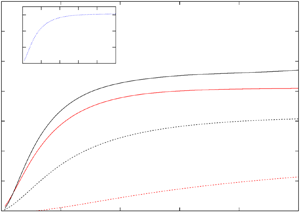
Figure 3. A sample of  $20$ simulations with white noise initial perturbations (thin red curves) with an average Reynolds number
  $Re =230$. The ensemble average is the thick black curve. These simulations are conducted on the linear evolutions of the perturbations.
  $\delta (t)$ is the energy norm defined in (2.5). We observe the same behaviour as in figure 2.
In figure 4, we show the dependence of the nonlinear amplifications of perturbations up to the time  $t = 0.3 T_0$ on the Reynolds number, where
  $T_0$ is the large eddy turnover time which is around
  $2$. The data fit well with
  $\textrm {e}^{c\sqrt {Re}}$ as we predicted in (1.1). Our numerical experiments show that this
  $\sqrt {Re}$-nature is generic with respect to the perturbations and the base solutions in homogeneous isotropic turbulence. Thus both the
  $\sqrt {t}$ and the
  $\sqrt {Re}$ features in the exponent of our prediction (1.1) are verified here in homogeneous isotropic turbulence regime.

Figure 4. The Reynolds number dependence of the nonlinear amplifications of perturbations up to the time  $t = 0.3 T_0$, where
  $T_0$ is the large eddy turnover time which is around
  $2$. Here,
  $\varDelta (t)$ is the energy norm defined in (2.4). The dashed curve is a fit to
  ${\sim } \sqrt {Re}$, and the red curve is a fit to
  ${\sim } Re^{0.38}$. Both the horizontal and vertical axes are in logarithmic scales.
3. Conclusion
In conclusion, built upon our earlier low resolution numerical simulations of our prediction (1.1) on the maximal amplification of perturbations in fully developed turbulence (Feng & Li Reference Feng and Li2020), here, we conduct large direct numerical simulations with sufficient resolutions on fully developed homogeneous isotropic turbulence, and we have verified our prediction (1.1). In particular, our numerical simulations show that the amplification of perturbations behaves as  $\textrm {e}^{c\sqrt {t}}$ in
  $t$ and
  $\textrm {e}^{c\sqrt {Re}}$ in
  $Re$ as we predicted in (1.1). These features are generically observed with respect to perturbations and base solutions. Thus amplifications of perturbations in fully developed turbulence are much faster than exponential in contrast to the exponential amplifications of perturbations in chaos. This suggests that the onset of fully developed turbulence should be more abrupt than low-dimensional chaos, and fully developed turbulence should appear more violent than low-dimensional chaos. Such superfast amplifications of perturbations naturally lead to superfast nonlinear saturation, and we have demonstrated that the nonlinear saturation is indeed superfast. Our results suggest that fully developed turbulence is generated, developed and maintained by such constant superfast amplifications and superfast nonlinear saturation of ever existing perturbations. We believe that this theory better explains what is observed in fully developed turbulence than the chaos theory.
We believe that our discovery here will better guide turbulence engineering, design and predictions such as ensemble weather forecasting in meteorology.
Acknowledgements
This work has used resources from the Edinburgh Compute and Data Facility (http://www.ecdf.ed.ac.uk) and ARCHER (http://www.archer.ac.uk). A.B. acknowledges support from the UK Science and Technology Facilities Council whilst R.D.J.G.H. is supported by the UK Engineering and Physical Sciences Research Council (EP/M506515/1).
Declaration of interests
The authors report no conflict of interest.
Appendix A
In this appendix, we give a brief description on the derivation of the maximal amplification estimate (1.1) obtained in Li (Reference Li2014). Starting from the Navier–Stokes equations
 \begin{equation} \left.\begin{gathered} u_t + \frac{1}{Re} {\rm \Delta} u = - \boldsymbol{\nabla} p - u\boldsymbol{\cdot} \boldsymbol{\nabla} u , \\ \boldsymbol{\nabla} \boldsymbol{\cdot} u = 0 , \end{gathered}\right\} \end{equation}
where  $u$ is the
  $d$-dimensional fluid velocity (
 $d=2,3$),
  $p$ is the fluid pressure and
  $Re$ is the Reynolds number. Applying the Leray projection, one gets
 \begin{equation} u_t + \frac{1}{Re} {\rm \Delta} u = - \mathbb{P} \left ( u\boldsymbol{\cdot} \boldsymbol{\nabla} u \right ) . \end{equation}
The Leray projection is an orthogonal projection in  $L^2(\mathbb {T}^d)$, given by
 \begin{equation} \mathbb{P} g = g - \boldsymbol{\nabla} \varDelta^{-1} \boldsymbol{\nabla} \boldsymbol{\cdot} g . \end{equation}
Applying the method of variation of parameters, one converts the Navier–Stokes equation (A 2) into the integral equation
 \begin{equation} u(t) = \exp({({t}/{Re})\varDelta}) u(0) - \int_0^t \exp({(({t-\tau})/{Re})\varDelta }) \mathbb{P} \left ( u\boldsymbol{\cdot} \boldsymbol{\nabla} u \right)\textrm{d}\tau . \end{equation}
Taking the differential in  $u(0)$ (which is the initial infinitesimal perturbation), one gets the differential form
 \begin{equation} \textrm{d}u(t) = \exp({({t}/{Re})\varDelta }) \,\textrm{d}u(0) - \int_0^t \exp({(({t-\tau})/{Re})\varDelta }) \mathbb{P} \left ( \textrm{d}u\boldsymbol{\cdot} \boldsymbol{\nabla} u +u \boldsymbol{\cdot} \boldsymbol{\nabla} \,\textrm{d}u \right ) \textrm{d}\tau . \end{equation}
First, we will derive the following inequality which will be used in estimating the above differential form
 \begin{equation} \| \exp({({t}/{Re})\varDelta }) u \|_n \leq \left (\frac{1}{\sqrt{2e}} \sqrt{\frac{Re}{t}} + 1 \right )\| u \|_{n-1} , \end{equation}
where  $\| \ \|_n$ represents the Sobolev
  $H^n$ norm. Notice that using the Fourier coefficients
  $u_k$ of
  $u$, we have
 \begin{align} \| \exp({({t}/{Re})\varDelta})u\|_n^2 &= \sum_{k \in \mathbb{Z}^3}(1+|k|^2+\cdots +|k|^{2n}) \exp({-({2t}/{Re})|k|^2})|u_k|^2 \nonumber\\ &= \sum_{k \in \mathbb{Z}^3}[\exp({-({2t}/{Re})|k|^2}) + \exp({-({2t}/{Re})|k|^2})|k|^2 (1+|k|^2 \nonumber\\ &\quad +\cdots +|k|^{2(n-1)}) ]|u_k|^2 \nonumber\\ &\leq \sum_{k \in \mathbb{Z}^3}[1+ \exp({-({2t}/{Re})|k|^2})|k|^2 (1+|k|^2 \nonumber\\ &\quad +\cdots +|k|^{2(n-1)}) ]|u_k|^2. \end{align}
Now we estimate  $\exp ({-({2t}/{Re})|k|^2})|k|^2$. Define
 \begin{equation} f(\xi) = \exp({-({2t}/{Re})\xi}) \xi , \quad \xi \in [0, +\infty ). \end{equation}
The critical point of  $f(\xi )$ is given by
 \begin{equation} \frac{\textrm{d}}{\textrm{d}\xi} f(\xi) = \exp({-({2t}/{Re})\xi}) \left ( 1-\frac{2t}{Re}\xi \right ) = 0 . \end{equation}
Thus
 \begin{equation} \xi = \frac{Re}{2t} \end{equation}
is the critical point. Since
 \begin{equation} \lim_{\xi \rightarrow +\infty} f(\xi) = 0, \quad f(0) = 0, \end{equation}
the critical point is a maximal point. Thus
 \begin{equation} f(\xi) \leq f\left(\frac{Re}{2t}\right) = \frac{1}{e} \frac{Re}{2t}, \quad \xi \in [0, +\infty ). \end{equation}
Using this fact in (A 7), we get
 \begin{align} \| \exp({({t}/{Re})\varDelta})u\|_n^2 &\leq \sum_{k \in \mathbb{Z}^3}\left[ 1+ \frac{1}{e} \frac{Re}{2t}(1+|k|^2+ \cdots +|k|^{2(n-1)}) \right]|u_k|^2\nonumber\\ &\leq \left ( 1+ \frac{1}{e} \frac{Re}{2t} \right )\sum_{k \in \mathbb{Z}^3}(1+|k|^2+\cdots +|k|^{2(n-1)}) |u_k|^2 \nonumber\\ &= \left ( 1+ \frac{1}{e} \frac{Re}{2t} \right ) \|u\|_{n-1}^2. \end{align}
Thus
 \begin{equation} \| \exp({({t}/{Re})\varDelta})u\|_n \leq \left ( 1+ \frac{1}{\sqrt{2e}} \sqrt{\frac{Re}{t}} \right ) \|u\|_{n-1} , \end{equation}
which is the inequality (A 6). With this inequality, we can estimate the Sobolev  $H^n$ norm of the integrand in (A 5). For example,
 \begin{equation} \| \exp({(({t-\tau})/{Re})\varDelta}) \mathbb{P} (\textrm{d}u \boldsymbol{\cdot} \boldsymbol{\nabla} u)\|_n \leq \left (\frac{1}{\sqrt{2e}} \sqrt{\frac{Re}{t-\tau}} +1 \right ) \| \mathbb{P} (\textrm{d}u \boldsymbol{\cdot} \boldsymbol{\nabla} u) \|_{n-1} . \end{equation}
It is easy to see that
 \begin{equation} \| \mathbb{P} (\textrm{d}u \boldsymbol{\cdot} \boldsymbol{\nabla} u) \|_{n-1} \leq 2 \| (\textrm{d}u \boldsymbol{\cdot} \boldsymbol{\nabla} u) \|_{n-1}. \end{equation}
In our specific setting,
 \begin{equation} \| (\textrm{d}u \boldsymbol{\cdot} \boldsymbol{\nabla} u) \|_{n-1} \leq c\| \textrm{d}u \|_{n-1} \| \boldsymbol{\nabla} u \|_{n-1} \leq c \| \textrm{d}u\|_n \|u\|_n , \end{equation}
where  $c$ only depends on
  $n$ and the spatial domain. Collecting all these estimates, one gets
 \begin{equation} \| \textrm{d}u(t) \|_n \leq \| \textrm{d}u(0) \|_n + 4c \max_{\tau \in [0,T]} \| u(\tau )\|_n \int_0^t \left ( \frac{\sqrt{Re}}{\sqrt{2e}} \frac{1}{\sqrt{t-\tau }} +1 \right )\| \textrm{d}u(\tau ) \|_n \,\textrm{d}\tau . \end{equation}
Applying the Gronwall's inequality, one gets the estimate
 \begin{equation} \| \textrm{d}u(t) \|_n \leq \exp({\sigma \sqrt{Re} \sqrt{t}+ \sigma_1 t}) \| \textrm{d}u(0) \|_n , \end{equation}
where
 \begin{equation} \sigma = \frac{8c}{\sqrt{2e}} \max_{\tau \in [0,T]} \| u(\tau )\|_n, \quad \sigma_1 = 4c \max_{\tau \in [0,T]} \| u(\tau )\|_n = \frac{\sqrt{2e}}{2} \sigma . \end{equation}
Thus,
 \begin{equation} \sup_{\textrm{d}u(0)} \frac{\| \textrm{d}u(t)\|_n}{\| \textrm{d}u(0)\|_n} \leq \exp({\sigma \sqrt{Re} \sqrt{t}+ \sigma_1 t}), \end{equation}
which is the maximal amplification estimate (1.1).
Appendix B
In this appendix, we show the longer time simulations of figure 3. In order to run for a longer time, we conduct a sample of  $11$ instead of
  $20$ simulations in figure 5. Using a log scale for the vertical axis, we can see that, around
  $t=10$, the exponential growth rate is approximately
  $0.6$ which is close to the value
  $0.59$ obtained in Berera & Ho (Reference Berera and Ho2018) (when using our current setting). Around
  $t=35$, the exponential growth rate is approximately
  $0.031$.

Figure 5. The longer time simulation of figure 3 with a sample of  $11$. The vertical axis is in log scale.


