


1. Introduction
Vorticity is well recognized to play a fundamental role in turbulent flows and its ultimate origin lies quite frequently at solid walls or flow boundaries. It therefore becomes a basic question to understand how vorticity in the interior of the flow evolved from vorticity generated at the wall. Recent mathematical work of Constantin & Iyer (Reference Constantin and Iyer2008, Reference Constantin and Iyer2011) has provided new exact tools to answer this question in terms of stochastic Lagrangian particle trajectories evolved backward in time. In the previous work by Eyink, Gupta & Zaki (Reference Eyink, Gupta and Zaki2020) – hereafter referred to as Part 1 – it was shown that the mathematical representations of Constantin & Iyer (Reference Constantin and Iyer2008, Reference Constantin and Iyer2011) have a simple fluid dynamical interpretation in terms of the ‘vortex-momentum density’ associated to a continuous distribution of infinitesimal vortex rings, which is the basis of the Kuz'min (Reference Kuz'min1983)–Oseledets (Reference Oseledets1989) formulation of the incompressible Navier–Stokes equation. For smooth ideal Euler solutions, the vortex-momentum density is Lie transported by the fluid flow as a 1-form and its curl, the vorticity, is transported as a 2-form (Oseledets Reference Oseledets1989; Tur & Yanovsky Reference Tur and Yanovsky1993). This Lie transport leads naturally to the vorticity invariants of Cauchy (Reference Cauchy1815) for incompressible Euler solutions and to generalized Cauchy invariants for the vortex-momentum density (Tur & Yanovsky Reference Tur and Yanovsky1993; Besse & Frisch Reference Besse and Frisch2017). The mathematical theory of Constantin & Iyer (Reference Constantin and Iyer2008, Reference Constantin and Iyer2011) provides corresponding ‘stochastic Cauchy invariants’ for Navier–Stokes solutions that are conserved on average by the stochastic Lagrangian flow backward in time and these invariants provide an explicit representation of the vortex-momentum density and the vorticity in terms of boundary data. We furthermore discussed in Part 1 some relations of the Constantin & Iyer (Reference Constantin and Iyer2008, Reference Constantin and Iyer2011) stochastic Lagrangian representation with the Eulerian theory of Lighthill (Reference Lighthill1963)–Morton (Reference Morton1984) for vorticity generation at solid walls and with an exact statistical result of Taylor (Reference Taylor1932)–Huggins (Reference Huggins1994) for the ‘vorticity flux tensor’. The latter is an anti-symmetric tensor  $\Sigma _{ij},$ which represents the flux of the
  $j$th component of the vorticity in the
  $i$th coordinate direction and which was observed by Huggins (Reference Huggins1994) (following Taylor (Reference Taylor1932) for a two-dimensional pipe flow) to have a mean value directly proportional to the mean pressure gradient in the
  $k$th direction, with
  $i,$
$i,$ $j,$
$j,$ $k$ all distinct. This relation applies to drag generally for any flows driven by imposed pressure gradients and/or free stream velocity, such as turbulent shear layers and wakes (Brown & Roshko Reference Brown and Roshko2012). The ‘vorticity source’ of Lighthill (Reference Lighthill1963) and Morton (Reference Morton1984) is defined at the wall by the vector
  $\sigma _i=\Sigma _{ij} \hat {n}_j,$ summed over repeated index
  $j,$ where
  $\hat {{\boldsymbol {n}}}$ is the outward-pointing unit normal vector on the boundary (Lyman Reference Lyman1990; Eyink Reference Eyink2008).
The main result that we exploit in the present work is the relation (Part 1, (2.51))
 \begin{equation} {\boldsymbol{\omega}}({ \boldsymbol{x} },t) = {\mathbb{E}}\left[\widetilde{{\boldsymbol{\omega}}}_s({ \boldsymbol{x} },t)\right], \quad s < t, \end{equation}
which expresses the vorticity vector at space–time point  $({ \boldsymbol {x} },t)$ as an expectation
  ${\mathbb {E}}$ of the stochastic Cauchy invariant
  $\widetilde {{\boldsymbol {\omega }}}_s({ \boldsymbol {x} },t)$ (Part 1, (2.55)). This is a random vector that can be evaluated along stochastic Lagrangian particle trajectories satisfying
 \begin{equation} \hat{\textrm{d}} { \widetilde{\boldsymbol{A}} }^s_t({ \boldsymbol{x} }) = { \boldsymbol{u}}({ \widetilde{\boldsymbol{A}} }^s_t({ \boldsymbol{x} }),s) \, \textrm{d} s + \sqrt{2\nu}\, \hat{\textrm{d}}{\widetilde{\mathbf{W}}}(s),\enspace s < t;\quad { \widetilde{\boldsymbol{A}} }^t_t({ \boldsymbol{x} })={ \boldsymbol{x} }, \end{equation}
which are released at  $({ \boldsymbol {x} },t)$ and move backward in time
  $s.$ Here
  ${\widetilde {\mathbf {W}}}(s)$ is a random Wiener process that represents diffusion by molecular viscosity. For every realization of the process, there is a largest time
  $s=\widetilde {\sigma }_t({ \boldsymbol {x} })$ at which the stochastic particle first hits the wall, backward in time. Each particle is stopped at the wall where it first hits and in that particular realization
  $\widetilde {{\boldsymbol {\omega }}}_s({ \boldsymbol {x} },t)=\widetilde {{\boldsymbol {\omega }}}_{\widetilde {\sigma }_t({ \boldsymbol {x} })}({ \boldsymbol {x} },t)$ for
  $s<\widetilde {\sigma }_t({ \boldsymbol {x} }),$ thus remaining fixed at earlier times. If one considers
  $s\ll t$ then the inequality
  $s<\widetilde {\sigma }_t({ \boldsymbol {x} })$ will hold with near certainty and, in that case, (1.1) represents the interior vorticity in terms of wall vorticity which is transported to
  $({ \boldsymbol {x} },t)$ by advection, diffusion and stretching. A numerical Monte Carlo Lagrangian algorithm was also developed in Part 1 to calculate realizations of the stochastic Cauchy invariants and their statistics, given a Eulerian space–time solution of the incompressible Navier–Stokes equation.
Here we shall exploit that approach to make a first-of-its-kind numerical study of stochastic Lagrangian dynamics of vorticity in a turbulent channel flow at high Reynolds number. If we denote Cartesian coordinate directions as streamwise  $x,$ wall normal
  $y$ and spanwise
  $z,$ then statistical homogeneity in
  $x$ and
  $z$ and reflection symmetry in
  $y$ provide simplifications in long-time averages. In particular, the mean flux of spanwise vorticity vertically from the wall becomes independent of wall-normal location as a consequence of conservation,
  $\partial _y\overline {\Sigma }_{yz}=0,$ and is given by
 \begin{equation} \overline{\Sigma}_{yz}=\overline{v'\omega_z'-w'\omega_y'} -\nu \frac{\partial \overline{\omega}_z}{\partial y} = \frac{\partial\overline{p}}{\partial x} ={-}\frac{u_*^2}{h}<0,\end{equation}
where  $f':=f-\overline {f}$ defines fluctuation away from the long-time mean value and the velocity vector
  ${ \boldsymbol {u}}=(u,v,w),$ where
  $u_*$ is the friction velocity and
  $h$ is the channel half-height (Huggins Reference Huggins1994; Eyink Reference Eyink2008). According to (1.3) the constant flux of spanwise vorticity away from the wall is numerically equal to the rate of mean downstream pressure drop, which characterizes turbulent drag and dissipation. In this paper we shall study the Lagrangian dynamics of vorticity in the buffer layer of a turbulent channel flow, which is conventionally taken to be the layer of fluid at heights
  $y^+$ over the range
  $5 < y^+ < 30$ (Tennekes & Lumley Reference Tennekes and Lumley1972), with
  $y^+$ in dimensionless wall units (see § 2). We have both pragmatic and fundamental reasons to focus on the buffer layer. Since all interior flow vorticity traces its origin back to a solid wall, the ‘youngest’ vorticity must lie closest to the wall. This makes the near-wall region numerically easiest to study by our approach. There is also motivation to understand the turbulent physics close to the wall, since one can expect that control of vorticity creation and transport at the earliest stage will be most efficient in reducing drag (Koumoutsakos Reference Koumoutsakos1999; Zhao, Wu & Luo Reference Zhao, Wu and Luo2004). On the other hand, nonlinear contributions to the dynamics are subleading (on average) in the viscous sublayer
  $y^+<5,$ and nonlinear contributions to mean vorticity transport first become substantial in the buffer layer.
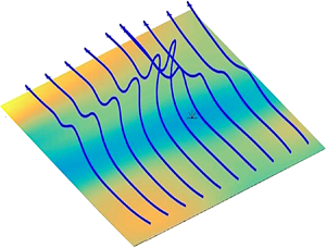
Our study is directly motivated by laboratory experiments of Sheng, Malkiel & Katz (Reference Sheng, Malkiel and Katz2009), who investigated buffer-layer structures in a turbulent square-duct channel flow at  $Re_\tau =1470$ using a technique of digital holographic microscopy that yields well-resolved measurements of three-dimensional velocity and velocity gradient fields. Conditional sampling based on local wall shear-stress maxima and minima revealed two types of structures that generate such extreme stress events; in accord with common terminology, these may be called ‘sweeps’ and ‘ejections’, respectively. The latter type of flow event generates arrays of vortex lines with a simple ‘hairpin’ structure that rise in an arch above the location of the wall stress minimum; see figure 1, which represents well the typical geometry of vortex lines observed by Sheng et al. (Reference Sheng, Malkiel and Katz2009) during an ‘ejection’. These raised vortex lines with a non-vanishing vertical component of vorticity are the signature closest to the wall of a contribution by nonlinear stretching and rotation to transport of spanwise vorticity upward from the wall. Such an orderly spatial array of lines as illustrated in figure 1 invites interpretation in terms of a similarly simple temporal progression, with each line apparently ‘moving’ forward and evolving into its downstream neighbour. Indeed, Sheng et al. (Reference Sheng, Malkiel and Katz2009) on the basis of such spatial arrays of lines (see their figures 7 and 21) have proposed an ‘abrupt lifting’ of vorticity in just one viscous time or, spatially, in a short distance of 10 wall units, above the location of a local stress minimum.

Figure 1. A typical array of vortex lines pointing spanwise and lifting in an arch over a low-speed streak at a wall stress minimum during an ‘ejection’ event in the buffer layer of a turbulent boundary layer. The wide arrow indicates the direction of the mean flow.
As we shall show by detailed Lagrangian analysis exploiting the stochastic Cauchy invariants, the deceptively simple Eulerian picture of vortex lines in figure 1 is in fact the outcome of a hidden, violent conflict between intense nonlinear stretching and rotation of vorticity vector elements on the one hand, and vigorous destruction of vorticity by viscosity on the other. Previous work by Johnson et al. (Reference Johnson, Hamilton, Burns and Meneveau2017) has demonstrated existence of Lagrangian chaos in channel-flow turbulence, which leads to rapid exponential stretching of material line elements. This poses a theoretical puzzle, however, because such stretching should lead to unbounded growth of vorticity, but the channel flow nevertheless attains a statistical steady state with a saturated magnitude of vorticity. The obvious mechanism that limits vortex stretching is viscous destruction (Taylor Reference Taylor1938), but advection and diffusion of same-sign vorticity cannot quench the growth due to stretching. We find that vorticity vector elements in the buffer layer are not only exponentially magnified, but also strongly rotated, so that they often point opposite to the negative spanwise direction pictured in figure 1. Cancellation of this oppositely directed vorticity by viscous diffusion leads to the regular geometry in figure 1. Furthermore, we find that the vortex lifting is not an ‘abrupt’ discrete event, but is instead a highly distributed process spread over more than 100 viscous times and 1000 wall units.
These results are obtained by a numerical study using an online computational dataset of channel-flow turbulence at  $Re_\tau =1000$ (Graham et al. Reference Graham, Kanov, Yang, Lee, Malaya, Lalescu, Burns, Eyink, Szalay and Moser2016). The accuracy of this database to study buffer-layer physics has been carefully evaluated and documented in Part 1, as briefly summarized in § 2. Our study not only yields new insights into Lagrangian vorticity dynamics of pressure-driven wall-bounded flows, but also reveals many common features of classical fluids and quantum superfluids, especially for wall-bounded turbulent flows through pipes and channels. To mention here just a few of these similarities, the Kuz'min (Reference Kuz'min1983)–Oseledets (Reference Oseledets1989) representation of the classical fluid by the vortex-momentum density is closely related to intuitive pictures of ‘vortex tangles’ in superfluids as superpositions of small vortex rings (Campbell Reference Campbell1972; Schwarz Reference Schwarz1982; Kuz'min Reference Kuz'min1999). Perhaps most importantly, Huggins (Reference Huggins1994) has emphasized that (1.3) is the exact analogue of the ‘Josephson–Anderson relation’ in quantum fluids; see Josephson (Reference Josephson1962), Anderson (Reference Anderson1966), Packard (Reference Packard1998) and Varoquaux (Reference Varoquaux2015) for reviews. This relation provides the accepted explanation for effective drag in an otherwise non-dissipative superfluid by cross-stream motion of quantized vortex lines. For further discussions of this analogy, see also Huggins (Reference Huggins1970) and Eyink (Reference Eyink2008). We argue briefly in the conclusion of the present paper that such similarity should extend to Lagrangian dynamics of vorticity and that the motion of ‘bundles’ of quantized vortex lines in turbulent superfluids should be also intrinsically stochastic.
The contents of this paper are outlined as follows. Section 2 summarizes the essentials of our numerical methods, which are described more completely in Part 1. Section 3 explains how the two specific flow events were selected for examination (3.1) and then describes both the ejection (3.2) and sweep (3.3) events in detail in conventional Eulerian terms. Our novel Lagrangian analysis is presented in § 4, where we first choose specific vorticity vectors for quantitative study (4.1) and then determine their dynamical origin at the wall for both the ejection (4.2) and the sweep (4.3). Finally, § 5 summarizes our results and conclusions, especially on common features of wall-bounded turbulence in classical fluids and quantum superfluids. Additional material that complements the discussion in the main text is provided as supplemental materials available at https://doi.org/10.1017/jfm.2020.492.
2. Numerical methods
We review here for completeness some necessary information about our computational approach from Part 1, which should be consulted for full details. The Johns Hopkins turbulence databases (JHTDB) channel-flow dataset (Graham et al. Reference Graham, Kanov, Yang, Lee, Malaya, Lalescu, Burns, Eyink, Szalay and Moser2016) is exploited for the empirical study in this paper. This data was generated from a Navier–Stokes simulation in a channel using a pseudospectral method in the plane parallel to the walls and a seventh-order B-splines collocation method in the wall-normal direction (Lee, Malaya & Moser Reference Lee, Malaya and Moser2013). For a numerical solution, the Navier–Stokes equations were formulated in wall-normal velocity–vorticity form (Kim, Moin & Moser Reference Kim, Moin and Moser1987). Pressure was computed by solving the pressure Poisson equation only when writing to disk, which was every five time steps for 4000 snapshots, enough for about one domain flow-through time. The simulation domain  $[0,8{\rm \pi} h] \times [-h,h] \times [0,3{\rm \pi} h],$
 $h=1,$ was discretized using a spatial grid of
  $2048 \times 512 \times 1536$ points. Time advancement was made with a third-order low-storage Runge–Kutta method and dealiasing was performed with 2/3 truncation (Orszag Reference Orszag1971). A constant pressure head was applied to drive the flow at
  $Re_\tau = 1000$ (
 $Re_{bulk} = {2hU_{bulk}}/{\nu } = 40\,000$) with bulk velocity near unity. As is common, we shall indicate with a superscript ‘
 $+$’ non-dimensionalized quantities in viscous wall units, with velocities scaled by friction velocity
  $u_*$ and lengths by viscous length
  $\delta _\nu =\nu /u_*=10^{-3}.$ Also as usual, we define
  $y^+=(h\mp y)/\delta _\nu$ near
  $y=\pm h.$ In these units, the first
  $y$-grid point in the simulation is located at a distance
  ${\rm \Delta} y_1^+ = 1.65199\times 10^{-2}$ from the wall, while in the centre of the channel
  ${\rm \Delta} y_c^+ = 6.15507.$ Other numerical parameters are summarized in table 1.
Table 1. Simulation parameters for a turbulent channel-flow dataset.
In Part 1 we developed and tested a numerical Monte Carlo Lagrangian algorithm to calculate the stochastic Cauchy invariants and their statistics, by discretizing the stochastic ordinary differential equation (1.2) with a step size  ${\rm \Delta} s$ and by averaging over
  $N$ independent realizations
  ${\widetilde {\mathbf {W}}}^{(n)}(s),$
 $n=1,\ldots ,N$ of the Wiener process. We showed in that work for the two specific cases from the JHTDB channel-flow dataset studied in the present paper that
  ${\rm \Delta} s=10^{-3}$ and
  $N=10^{7}$ sufficed to give converged results for the mean and variance of the stochastic Cauchy invariant over a time interval
  $-100<\delta s^+<0$ with
  $\delta s:=s-t.$ In particular, it was shown that the mean conservation law (1.1) holds for those two cases to within a few per cent over that time interval, which is a quite stringent test of validity of our numerics. The residual errors in the mean conservation can be explained by some near wall under resolution of the numerical JHTDB data, indicated by the sizable
  ${\rm \Delta} x^+$ and
  ${\rm \Delta} z^+$ values in table 1, and by errors in the finite-difference approximation of velocity gradients within the database. To test that hypothesis, we also spatially coarse grained the relation (1.1) over
  $n_i$ grid spacings in each of the coordinate directions
  $i=x,y,z,$ since such coarse-grained fields from the JHTDB dataset should represent better a coarse-grained Navier–Stokes solution. We verified that such coarse graining noticeably improves mean conservation, in particular, for
  $(n_x,n_y,n_z)=(4,0,4).$
In §§ 3.1 and 4.1, below, we describe the criteria that we used to select the two test cases for study in this work. In particular, we discuss in § 3.1 how a pair of events, an ‘ejection’ and a ‘sweep’, were identified in the Eulerian dataset, following the work of Sheng et al. (Reference Sheng, Malkiel and Katz2009). In § 4.1 we then describe how we selected a space–time point  $({ \boldsymbol {x} },t)$ in each event for comparative study by stochastic Lagrangian analysis. We also show there that coarse graining the JHTDB fields with
  $(n_x,n_y,n_z)=(4,0,4)$ does not change qualitatively the Eulerian and Lagrangian picture of the two events. These results, together with those presented in Part 1, validate both our Monte Carlo numerical method to calculate the stochastic Cauchy invariant and also the adequacy of the JHTDB channel-flow database to resolve the physics of the turbulent buffer layer.
3. Eulerian vorticity dynamics in the buffer layer
3.1. Identification of ejections and sweeps
Following the approach of Sheng et al. (Reference Sheng, Malkiel and Katz2009), we selected events where the viscous shear stress  $\tau _{xy}=\nu (\partial u/\partial y)$ at the wall has local minima and local maxima with magnitudes satisfying a threshold condition. For this purpose, we downloaded the stress field at the entire top wall of the channel-flow database at the final archived time
  $t_f=25.9935$ and searched for local minima and maxima. Note that we used the data at the top wall because the bottom wall data was temporarily unavailable when we began our study; in order to present our results below we always rotate the figures
  $180^\circ$ around the streamwise axis, so that the top wall is exchanged with the bottom wall. In supplementary material we provide a plot of the normalized stress field
  $\tau _{xy}^+=\tau _{xy}/u_*^2$ over the entire channel wall and a probability density function (PDF) of its values, which range from
  $-2.55$ to
  $+7.54$ and have mean value unity. To find local minima and maxima, we used a fast peak finder for two-dimensional scalar data (Natan Reference Natan2013). We found that the points identified by this code for field
  $\tau _{xy}$ were indeed local maxima and for
  $-\tau _{xy}$ were local minima, but that weaker maxima/minima were often missed. We therefore do not regard the output of this algorithm to be completely reliable to obtain statistics of the local extrema, but it suffices for our purpose of identifying specific local maxima/minima. Nevertheless, we do provide in the supplementary material for the interest of readers the obtained PDF's of the stress values at the positions both of the local minima and also of the local maxima. The PDF of the local minimum stress values shows a large peak at
  $\tau _p^+\doteq 0.6,$ while the PDF of the local maximum stress values shows a large peak at
  $\tau _p^+\doteq 1.8.$ Interestingly, the condition that Sheng et al. (Reference Sheng, Malkiel and Katz2009) applied to identify ‘extreme stress events’ was
  $\tau _{xy}^+<0.6$ for local minima and
  $\tau _{xy}^+>1.8$ for local maxima, in good agreement with these peaks values. We therefore searched for two typical events of this type, namely, for a local minimum of stress with value
  $\tau _{xy}^+\doteq 0.6$ and for a local maximum of stress with value
  $\tau _{xy}^+\doteq 1.8.$ We also looked for such local extremum points which were relatively isolated from others. After examining several candidates, we selected as representative the two local extrema with database space–time coordinates given in table 2. The reader will note that these coordinates correspond, as stated above, to points on the top wall of the channel. The reader should transform results in Part 1 according to
  $(\omega _x,\omega _y,\omega _z)\to (\omega _x,-\omega _y,-\omega _z)$ for consistency with visualizations in the present paper. In particular, mean spanwise vorticity
  $\overline {\omega }_z$ under this transformation becomes negative.
Table 2. Coordinates of local minimum and local maximum wall stress events.

We shall refer to the local minimum stress event as an ‘ejection’ and to the local maximum stress event as a ‘sweep.’ This terminology is in agreement with the classification of Sheng et al. (Reference Sheng, Malkiel and Katz2009) in their table 2, but it differs somewhat from the most common characterization of such structures based on quadrant analysis in the  $(u',v')$ velocity plane, with connected regions of Q2 fluctuations designated as ‘ejections’ and regions of Q4 fluctuations as ‘sweeps’ (Jiménez Reference Jiménez2013). As we shall see from a detailed Eulerian description of these two selected events in the following §§ 3.2 and 3.3, our use of the terms ‘ejection’ and ‘sweep’ is not unrelated with the traditional quadrant analysis. We have purposely avoided using the term ‘burst’ to describe either of our two events, although ‘ejections’ have sometimes in the past been equated with ‘bursts.’ In more current understanding, however, buffer-layer ‘bursting’ is believed to be associated with quasi-periodic breakdown of unstable coherent structures presumably described by travelling wave solutions of Navier–Stokes equations (Jiménez (Reference Jiménez2013), sections IV.A–B; Park, Shekar & Graham Reference Park, Shekar and Graham2018). The quasi-period of this bursting is expected to be
  $\simeq 400$ viscous times
  $t_\nu =\nu /u_*^2$ with duration
  $\simeq 100$ viscous times, during which the travelling structure evolves from a low wall stress to high wall stress state; see, for example, Jiménez (Reference Jiménez2013), figure 10, or Park et al. (Reference Park, Shekar and Graham2018), figure 6. Therefore, ‘ejections’ and ‘sweeps’ in our sense may both be associated with buffer-layer bursting, at different stages in the evolution of the burst. Our interest here is mainly in analysing the Lagrangian dynamics of vorticity within these two buffer-layer events and not in determining their relation with ‘bursting’.
In §§ 3.2 and 3.3 we first provide a detailed description of these events in Eulerian terms. This does illuminate some connections with ‘bursting’, but our primary purpose is to describe these two events in terms of standard Eulerian theory of vorticity generation at walls and to compare with prior numerical and experimental results. Among these, we wish to compare our chosen events with those selected in Sheng et al. (Reference Sheng, Malkiel and Katz2009) by identical criteria and to verify that our events have the same characteristic features. In particular, we shall show that our ‘ejection’ event is quite typical of those studied by Sheng et al. (Reference Sheng, Malkiel and Katz2009) and used by them to postulate the ‘abrupt lifting’ of vortex lines. Here it is appropriate to make a remark on the relative importance of nonlinear dynamics and viscous diffusion for vorticity transport in the buffer layer. As stressed in the introduction, an ‘abrupt lifting’ event requires nonlinear stretching and rotation of spanwise vorticity in order to create a vertical arch. However, linear viscous diffusion dominates the mean vertical flux of spanwise vorticity not only in the viscous sublayer and buffer layer but even into the log layer! In fact, the simple relation
 \begin{equation} \overline{v'\omega_z'-w'\omega_y'} = \frac{\partial}{\partial y}\left(\overline{-u' v'}\right) \end{equation}
implies that the nonlinear contribution to spanwise vorticity flux is positive for  $y^+ < y^+_p,$ the location of the peak Reynolds shear stress
  $\overline {-u'v'}$ (Klewicki et al. Reference Klewicki, Fife, Wei and McMurtry2007; Eyink Reference Eyink2008). In the JHTDB channel-flow dataset at
  $Re_\tau =1000$ this peak occurs at about
  $y_p^+\doteq 50$ (Graham et al. Reference Graham, Kanov, Yang, Lee, Malaya, Lalescu, Burns, Eyink, Szalay and Moser2016). The net effect of the nonlinear terms for
  $y^+ < y^+_p$ is thus to transport spanwise vorticity opposite to the conserved total flux
  $\overline {\Sigma }_{yz}$ in (1.3), and viscous transport must be even more negative to compensate. We shall see also in the Lagrangian description that viscous diffusion plays an essential role in buffer-layer vorticity transport, even for extreme stress events where nonlinear terms are enhanced.
3.2. Eulerian description of ejection event
The stress local minimum that we selected for study is located within a long low-speed streak of the type commonly observed in near-wall turbulence, with typical spanwise separations  $\delta z^+\simeq 100$ between streaks (Jiménez Reference Jiménez2013). This environment is illustrated in figure 2, which plots the viscous shear stress
  $\tau _{xy}=\nu (\partial u/\partial y)$ at the wall, with magnitudes represented by the colour (or shade, in greyscale), together with the location of the stress local minimum as an asterisk ‘
 $*$’. This figure also plots the two-dimensional wall stress field
  ${\boldsymbol {\tau }}_W=\nu (\partial u/\partial y,\partial w/\partial y)$ with black arrows. The arrows indicate a near-wall, in-plane flow which is converging toward the streak. This convergence is consistent with a vertical flow that is upward, away from the wall, at the streak and it agrees with results of Sheng et al. (Reference Sheng, Malkiel and Katz2009) for the conditional average stress field in the vicinity of such local minima (see their figure 6f). More insight into the local flow conditions is provided by figure 3, which in panel (a) visualizes the coherent vortices in the vicinity of the local minimum using isosurfaces of
  $\lambda _2,$ or the second eigenvalue of the
  $({\boldsymbol {\nabla }}_x{ \boldsymbol {u}})^2$ matrix (Jeong & Hussain Reference Jeong and Hussain1995). Somewhat different choices of
  $\lambda _2$-levels and different vortex visualization criteria yield similar results. Clearly observed are two long, equal strength, streamwise vortices located on each side of the low-speed streak and inclined away from the wall. Measurement of
  $\omega _x$ reveals that these vortices are counter-rotating, generating a lifting flow above the low-speed streak. This is illustrated in figure 3(b), which provides a colour plot of
  $\omega _x$ in the transverse
  $y$-
$y$- $z$-plane through the middle of the visualized box and which also plots as arrows the two-dimensional cross-stream flow vectors
  $(w,v)$ within that plane. This type of counter-rotating vortex pair generating a lifting flow between them is a quite common buffer-layer configuration, encountered in about 16 % of all samples in the study of Sheng et al. (Reference Sheng, Malkiel and Katz2009) and in 98 % of their realizations satisfying the condition
  $\tau _{xy}^+<0.6.$ Our selected event thus appears to be quite typical of such stress minima and similar features were observed in many other local minima stress events that we identified in the JHTDB channel-flow dataset satisfying the criteria
  $\tau _{xy}^+\simeq 0.6.$

Figure 2. Field of viscous shear stress  $\tau _{xy}^+=(\partial u^+/\partial y^+)$ at the wall
  $y^+=0$ in wall units so that the average is unity. The black arrows represent the two-dimensional in-wall stress vector
  ${\boldsymbol {\tau }}_W.$ The asterisk ‘
 $*$’ marks the location of the selected stress local minimum.

Figure 3. (a) Isosurface  $\lambda _2^+=-0.0163,$ with a magnitude four times the local box-average value
  $\langle |\lambda _2^+|\rangle =4.09\times 10^{-3}.$ The shear-stress field from figure 2 is replotted in the bottom
  $x$-
$x$- $z$-plane for reference. (b) Field of streamwise vorticity
  $\omega _x^+$ in plane
  $x^+=85.9$ (transparent in panel (a)). The black arrows represent cross-stream velocity vectors
  $(w,v)$.
This typicality is confirmed by figure 4 which plots vortex lines crossing the visualized domain in the spanwise direction, initialized at evenly spaced streamwise locations and at initial elevations  $y^+=2,4,6,8.$ These vortex lines are lifted in arches above the low-speed streak, with a typical ‘hairpin’ geometry. The arches are nearly vertical for lines initiated at
  $y^+=2,4$ and also for
  $y^+=6,8$ at points well upstream of the stress minimum. For lines initiated at
  $y^+=6$, the arches rise and bend downstream approaching the stress minimum, while the lines initiated at
  $y^+=8$ near the stress minimum have instead an ‘
 $\Omega$-vortex’ geometry and the uppermost tips are bent back slightly upstream. These arrays of vortex lines are typical of those observed in the vicinity of stress local minima in the study of Sheng et al. (Reference Sheng, Malkiel and Katz2009), as illustrated in their figures 4(a), 8(a) for individual realizations and in their figure 7 for lines of the conditionally averaged vorticity field given
  $\tau _{xy}^+<0.6.$ Note that figure 4(c) plots the same vortex lines shown in figure 1 in the introduction. One of the primary goals of this work is to elucidate the surprisingly complex and violent Lagrangian dynamics underlying this simple vortex-line structure.

Figure 4. Vortex lines initiated at points with streamwise separations  ${\rm \Delta} x^+=12.3,$ with
  $z^+=128.8$ and (a)
  $y^+=2$, (b)
  $y^+=4$, (c)
  $y^+=6$, (d)
  $y^+=8.$ The shear-stress field from figure 2 is replotted in the bottom
  $x$-
$x$- $z$-planes for reference.
Further insight into the local vorticity dynamics from the Eulerian perspective is provided by results on the in-wall pressure distribution  $p(x,z)$, spanwise vorticity source
  $\sigma _z(x,z)$ and selected in-wall vortex lines, as plotted in figure 5 for the vicinity of our stress local minimum. Panel (a) of that figure reveals that our selected stress minimum is very close to a local pressure minimum, which in turn is flanked upstream and downstream at distances
  $\delta x^+\simeq \pm 60$ by a pair of local pressure maxima. The pressure isolines or isobars in this plot are the lines of instantaneous generation of tangential vorticity in the Lighthill–Morton theory, with positive (counterclockwise) sense of rotation around pressure maxima and negative (clockwise) rotation around pressure minima. Of course, these isobars align only with the direction of generation of vorticity and the instantaneous vortex lines within the wall are instead pointed mainly in the spanwise direction with small streamwise deviations, as shown in figure 5(b). The bending of these lines is explained in detail by the relation
  ${\boldsymbol {\tau }}_W=\nu \hat {{\boldsymbol {n}}}{ {\times }}{\boldsymbol {\omega }}_W$ between the in-wall stress and vorticity fields (Lighthill Reference Lighthill1963; Morton Reference Morton1984). As a consequence, the stress vectors
  ${\boldsymbol {\tau }}_W$ plotted in figure 2 are locally perpendicular to the in-wall vortex lines in figure 5(b) and the concavity of the lines is exactly that required to produce a converging flow at the low-speed streak. We plot in figure 5(b) as well the negative spanwise vorticity source
  $-\sigma _z^+ = -\partial p^+/\partial x^+ =\partial \omega _z^+/\partial y^+$ in wall units. We included the minus sign since drag evidenced by a streamwise drop in pressure is associated to flux of negative spanwise vorticity away from the wall. Thus, the colour/shading schemes in figures 2 and 5(b) are consistent, with yellow/light corresponding to increased drag (high stress, pressure drop) and blue/dark corresponding to reduced drag (low stress, pressure rise). Note, however, that the mean pressure drop associated to dissipative turbulent drag is
  $-\partial \overline {p}^+/\partial x^+=1/Re_\tau =10^{-3},$ whereas the instantaneous streamwise pressure gradients plotted in figure 5(b) are 100 times larger in magnitude, spanning a range from
  $-0.15$ to
  $+0.15$. It is consistent with the results in figure 5(b) that instantaneous pressure gradients at the wall scale as
  $u_*^2/\delta _\nu$ and, thus, remain
  $O(1)$ in wall units. The average streamwise pressure drop is thus the result of near cancellation between large instantaneous gradients of both signs.

Figure 5. (a) Pressure field  $p^+$ at the wall, with selected isolines in black. (b) The source field
  $-\sigma _z^+$ of the negative spanwise vorticity and selected in-wall vortex lines. The asterisk ‘
 $*$’ in both panels marks the location of the selected stress local minimum.
It is interesting to observe in figure 5(b) that a region of negative streamwise pressure gradient occurs just upstream of the stress local minimum and a corresponding region of positive gradient occurs just downstream. This seems to agree with experimental observations of ‘bipolar’ spanwise vorticity generation by Andreopoulos & Agui (Reference Andreopoulos and Agui1996) and Klewicki, Priyadarshana & Metzger (Reference Klewicki, Priyadarshana and Metzger2008), based on conditionally averaged time series of pressure and vorticity flux, and on time-correlation functions of pressure and pressure gradients. Andreopoulos & Agui (Reference Andreopoulos and Agui1996) proposed a conceptual model of ejections as rising ‘mushroom vortices’ that would produce exactly such a bipolar pattern of spanwise vorticity source at the wall; see Andreopoulos & Agui (Reference Andreopoulos and Agui1996), figure 28(b). However, a plot in figure 6 of the spanwise vorticity fluctuation  $\omega _z'$ and velocity vector fluctuation
  $(u',v')$ in the plane
  $z^+=85.9$ for our event is not consistent with such a picture. Panel (a) of that figure shows the entire
  $y^+$-range, for context, and panel (b) zooms into the near-wall region
  $y^+<10.$ To make the flow pattern more clear in figure 6(b), we have calculated fluctuations with respect to local planar averages at fixed distances
  $y^+$ from the wall (see supplementary material for details). We observe that the ‘bipolar’ source is produced by a fluid layer with
  $\omega _z'<0$ being lifted up and to the right from the bottom wall, while replacement fluid with
  $\omega _z'>0$ is advected in from the right and downward toward the wall. This dynamics is very similar to that postulated by Jimenez et al. (Reference Jimenez, Moin, Moser and Keefe1988, figure 6) as a mechanism of sublayer ejections. Those authors also observed thin, low-inclined layers of
  $\omega _z'$ like those in our figure 6(a) and interpreted them as Tollmien–Schlichting waves. Such shear layers are also inferred for coherent, nonlinear travelling waves (Waleffe Reference Waleffe1998, figure 1). Finally, Andreopoulos & Agui (Reference Andreopoulos and Agui1996) argued that ‘ejections which carry fluid of negative
  $\omega _z$ away from the wall
 $\ldots$are expected to be characterized by positive
  $\partial \omega _z/\partial y$. Negative
  $\partial \omega _z/\partial y$ is expected to be the distinguishing feature of sweeps
 $\ldots$’. The ejection event that we consider has near
  $y^+\simeq 5\text {--}10$ an upward flux of negative spanwise vorticity associated with
  $v'\omega _z'<0.$ However, there is no instantaneous balance between this advective flux and the viscous flux
  $\sigma _z=-\nu (\partial \omega _z/\partial y)$ at the wall. Thus, it is not clear that the region with
  $\partial \omega _z/\partial y>0$ upstream of the stress local minimum should be regarded as the ‘source’ of the advective spanwise vorticity flux at
  $y^+\simeq 5\text {--}10$. Our Lagrangian analysis in § 4 shall show indeed that there is no causal connection.

Figure 6. (a) Field of spanwise vorticity fluctuation  $\omega _z^{+\prime }$ in the
  $x$-
$x$- $y$-plane at
  $z^+=85.9.$ The black arrows represent the vectors
  $(u',v')$ of the cross-section velocity fluctuation. (b) Same as (a) but with fluctuations calculated relative to local planar averages at constant
  $y^+$ and plotted in the near-wall region
  $y^+<10$.
3.3. Eulerian description of sweep event
The stress local maximum that we selected for study is likewise located within a high-speed streak of a type also commonly observed in near-wall turbulence, generally shorter than the low-speed streaks in streamwise extent and flanking them (Jiménez Reference Jiménez2013). This neighbourhood is illustrated in figure 7, which plots the viscous shear stress  $\tau _{xy}=\nu (\partial u/\partial y)$ at the wall and the location of the stress local maximum as an asterisk ‘
 $*$’. The arrows representing the two-dimensional wall stress field
  ${\boldsymbol {\tau }}_W$ indicate a near-wall, in-plane flow which is diverging from the streak. This divergence is consistent with a vertical flow that is downward toward the wall at the streak and it agrees with results of Sheng et al. (Reference Sheng, Malkiel and Katz2009) for the conditional average stress field in the vicinity of such local maxima (see their figure 6e). Vortex visualization in figure 8(a) via
  $\lambda _2$-isosurfaces shows a more complex environment than for the preceding local minimum event. There are two or three large quasi-streamwise vortices at heights
  $y^+>20,$ but these do not seem to influence strongly the near-wall physics. Instead at elevations
  $y^+<20$ there is a pair of counter-rotating almost streamwise vortices, one on each side of the observed high-speed streak. The plot in figure 8(b) of streamwise vorticity
  $\omega _x$ and cross-stream velocity vectors
  $(w,v)$ in the transverse
  $y$-
$y$- $z$-plane cutting through the middle of the visualized box shows clearly that this low-lying pair generate a downward, splatting flow between them. Unlike the pair observed near the stress minimum, however, this pair is asymmetrical in strength, with the rightmost member of the pair distinctly weaker. If we increase the magnitude of the threshold value of
  $\lambda _2$ by even 33 % to
  $\lambda _2^+=-0.0143$ then no isosurface appears for this weaker vortex and only the single stronger vortex is observed at
  $y^+<20.$ This is consistent with the findings of Sheng et al. (Reference Sheng, Malkiel and Katz2009), who did encounter counter-rotating vortex pairs generating a splatting flow between them in 11 % of all of the samples in their study. However, under the condition
  $\tau _{xy}^+>1.8,$ only about 8 % of the realizations were of this type and all of these vortex pairs were quite asymmetrical in strength. Instead, 55 % of the realizations in the study of Sheng et al. (Reference Sheng, Malkiel and Katz2009) that satisfied the condition
  $\tau _{xy}^+>1.8$ had the stress maximum generated by a single low-lying vortex. Our selected event thus exhibits typical features for such stress maxima. Similar features were observed also in other local maxima stress events that we identified in the JHTDB channel-flow dataset satisfying the criteria
  $\tau _{xy}^+\simeq 1.8.$

Figure 7. Field of viscous shear stress  $\tau _{xy}^+=(\partial u^+/\partial y^+)$ at the wall
  $y^+=0$ in wall units so that the average is unity. The black arrows represent the two-dimensional in-wall stress vector
  ${\boldsymbol {\tau }}_W.$ The asterisk ‘
 $*$’ marks the location of the selected stress local maximum.

Figure 8. (a) Isosurface  $\lambda _2^+=-0.0107,$ with a magnitude three times the local box-average value
  $\langle |\lambda _2^+|\rangle =3.57\times 10^{-3}.$ The shear-stress field from figure 7 is replotted in the bottom
  $x$-
$x$- $z$-plane for reference. (b) Field of streamwise vorticity
  $\omega _x^+$ in plane
  $x^+=85.9$ (transparent in panel (a)). The black arrows represent cross-stream velocity vectors
  $(w,v)$.
The vortex lines that we observe near this stress local maximum likewise show expected features. See figure 9, which plots vortex lines crossing the visualized domain in the spanwise direction, initialized at evenly spaced streamwise locations and at initial elevations  $y^+=4,8,12,16.$ These lines are clearly squashed or depressed toward the wall by the downward splatting flow at the high-speed streak. Such arrays of vortex lines are typical of those observed in the vicinity of stress local maxima in the study of Sheng et al. (Reference Sheng, Malkiel and Katz2009), as illustrated in their figure 16 for individual realizations and in their figure 17 for lines of the conditionally averaged vorticity field given
  $\tau _{xy}^+>1.8.$ As they also observed, the ‘troughs’ of depressed lines are wider than the corresponding ‘hairpins’ above low-speed streaks. Also, the asymmetry in strength of the streamwise vortices is clearly visible, with the ridge of lines located at the strong vortex obviously twisted higher than those at the weak vortex. In § 4 we shall study in depth the Lagrangian dynamics of the illustrated squashed lines at the local maximum of stress.

Figure 9. Vortex lines initiated at points with streamwise separations  ${\rm \Delta} x^+=12.3,$ with
  $z^+=128.8$ and (a)
  $y^+=4$, (b)
  $y^+=8$, (c)
  $y^+=12$, (d)
  $y^+=16.$ The shear-stress field from figure 7 is replotted in the bottom
  $x$-
$x$- $z$-planes for reference.
First, however, we consider the vorticity dynamics for this event in more detail from the Eulerian perspective. The plot in figure 10(a) of the pressure field and its isolines at the wall shows that the stress maximum is close to a local pressure maximum, with a pair of local pressure minima upstream and downstream at distances  $\delta x^+\simeq \pm 80.$ In contrast to the instantaneous generation of vorticity along the isobars, the actual vortex lines at the wall plotted in figure 10(b) are aligned mainly in the spanwise direction. The lines bend in the streamwise direction so that the locally perpendicular stress vectors
  ${\boldsymbol {\tau }}_W,$ as plotted in figure 7, correspond to a near-wall flow diverging away from the high-speed streak. The negative spanwise vorticity source
  $-\sigma _z$ also plotted in figure 10(b) again shows a bipolar pattern of the type inferred by Andreopoulos & Agui (Reference Andreopoulos and Agui1996) and Klewicki et al. (Reference Klewicki, Priyadarshana and Metzger2008) from experimental data, with a region of positive streamwise pressure gradient occurring just upstream of the stress local maximum and a region of negative gradient just downstream. In the conceptual model of Andreopoulos & Agui (Reference Andreopoulos and Agui1996), figure 28(a), sweeps correspond to inverted ‘mushroom vortices’ moving toward the wall, producing just such a pattern of positive spanwise vorticity source upstream and negative spanwise source downstream. However, we do not observe such a mushroom vortex here. The plot in figure 11(a) of the spanwise vorticity fluctuation
  $\omega _z'$ and velocity vector fluctuation
  $(u',v')$ in the plane
  $z^+=79.7$ does exhibit a fluid layer near
  $y^+\simeq 10$ with
  $\omega _z'>0$ and
  $v'<0,$ associated with a spanwise vorticity flux
  $v'\omega _z'<0.$ However, this occurs mainly upstream from the stress local maximum, which is exactly opposite to what is proposed in the mushroom-vortex model. Figure 11(b) shows instead underneath the primary vortex with
  $\omega _z'>0$ a layer of strong secondary vorticity with
  $\omega _z'<0$ just above the wall. (Unlike for the ejection case earlier, the local plane average of streamwise velocity
  $u,$ used to define the fluctuation
  $u'$ in figure 11(b), is noticeably larger than the global average. See figure 11(a) and the supplementary material.) This secondary layer is apparently produced by a strong interaction of the primary vortex with the wall, as illustrated in figure 26 of Andreopoulos & Agui (Reference Andreopoulos and Agui1996), but the primary and secondary layers are not rolled up to form the head of a mushroom vortex. It is the presence of the secondary layer with
  $\omega _z'<0$ just above the wall that makes
  $\partial \omega _z/\partial y<0$ upstream of the stress local maximum, while the absence of such a secondary layer makes
  $\partial \omega _z/\partial y>0$ downstream. The thin, inclined layers of
  $\omega _z'$ observed in figure 11(a), although now for a sweep rather than an ejection, are again quite similar to those reported by Jimenez et al. (Reference Jimenez, Moin, Moser and Keefe1988), who also emphasized the important role of opposite-sign vorticity induced at the wall in producing such structures. These observations suggest some possible common features in viscous sublayer dynamics of ejections and sweeps. In the following § 4 we shall attempt to further explicate the physics of both types of events by stochastic Lagrangian analysis.

Figure 10. (a) Pressure field  $p^+$ at the wall, with selected isolines in black. (b) The source field
  $-\sigma _z^+$ of the negative spanwise vorticity and selected in-wall vortex lines. The asterisk ‘
 $*$’ in both panels marks the location of the selected stress local maximum.

Figure 11. Field of spanwise vorticity fluctuation  $\omega _z^{+\prime }$ in the
  $x$-
$x$- $y$-plane at
  $z^+=79.7.$ The black arrows represent the vectors
  $(u',v')$ of the cross-section velocity fluctuation. (b) Same as (a) but with fluctuations calculated relative to local planar averages at constant
  $y^+$ and plotted in the near-wall region
  $y^+<10$.
4. Stochastic Lagrangian dynamics of vorticity in the buffer layer
4.1. Selection of vorticity vectors
We now select for analysis specific vortex lines and specific vorticity vectors lying upon them. In this initial study we will compare the Lagrangian dynamics of two vorticity vectors both pointing approximately in the negative spanwise direction and located at points at a similar distance from the wall,  $y^+\simeq 5,$ at the bottom of the buffer layer. For the ejection event in particular, we want to investigate the initial nonlinear transfer of spanwise vorticity from the wall, which was described by Sheng et al. (Reference Sheng, Malkiel and Katz2009) as the process where ‘spanwise vorticity lifts abruptly from the wall, creating initially a vertical arch’. We have therefore considered for Lagrangian analysis in the ejection event the lowest-lying vortex lines in figure 4(a), which are replotted in figure 12(a). These lines all start on the right at height
  $y^+=2$ and then pass left in the negative spanwise direction, rising up in a nearly vertical arch over the low-speed streak. We chose the middle of these lines, coloured solid black, and, in particular, the vorticity vector at the top of the arch on that line at height
  $y^+=5.35,$ indicated by the arrow. For comparison, we considered in the sweep event the vortex lines which are squashed down to a comparable height above the wall by the splatting flow. This is the set of lines in figure 4(c), replotted in figure 12(b), which all start at
  $y^+=12$ and as they pass leftward are depressed in a trough above the high-speed streak. We chose the middle of these lines, coloured solid black, and, in particular, the vorticity vector at the bottom of the trough on that line at height
  $y^+=4.90,$ indicated by the arrow. The components of the two vorticity vectors and their position coordinates in the channel-flow database are recorded in table 3. Note that the vorticity vector for the sweep has a magnitude around twice that for the ejection. This is consistent with the argument of Lighthill (Reference Lighthill1963) that sweeps to the wall should stretch and magnify spanwise vorticity, while ejections should attenuate it (see his figure II.22).

Figure 12. The selected vortex lines, solid black, and the two selected vorticity vectors represented as arrows for (a) the ejection event and (b) the sweep event. Other vortex lines in the two flow events are plotted as dotted lines.
Table 3. Coordinates of analysed vorticity vectors.

Although the two vectors have different magnitudes, they are otherwise similar in orientation and in distance from the wall. This pair of vectors is thus well suited to illuminate differences in Lagrangian dynamics that arise solely from the different flow conditions that exist in the two events. In particular, our expectation is that the vorticity in the ejection event should have arisen recently from the wall and should be ‘younger’, while the vorticity at the same distance from the wall in the sweep event should be ‘older’ vorticity that entered from the wall at an earlier time, was processed by the flow, and was then returned by the splatting motion toward the wall. We shall see whether these expectations are borne out by our stochastic Lagrangian analysis.
We must first consider, however, the effect of filtering/coarse graining on the structure and dynamics of the two events pictured in figure 12. As discussed in § 2, the mean conservation law (1.1) obtained from the JHTDB simulation data would be expected to have improved validity when spatially coarse grained over  $n_i$ grid spaces in the three coordinate directions
  $i=x,y,z.$ This expectation was verified in Part 1 with a box filter; see figure 3 there for the ejection case and figure 5 for the sweep case. However, to justify the JHTDB channel-flow data as a Navier–Stokes solution accurate enough to investigate buffer-layer physics, it must also be shown that the filtering does not smear out the motions of interest. We have thus attempted to choose
  $(n_x,n_y,n_z)$ as small as possible, sufficient to verify that mean conservation is improved but not so large that the coarse graining obscures the essential physics. We have found that coarse graining in the
  $y$-direction does not help to improve mean conservation, presumably since the numerical resolution in the channel-flow simulation was sufficient in that direction, so that we take
  $n_y=0.$ By trial, we have found that a good choice of filtering lengths in the wall-parallel directions are
  $n_x=n_z=4,$ although somewhat smaller or larger values give similar results. Figure 13 verifies that the coarse-grained fields for
  $(n_x,n_y,n_z)=(4,0,4)$ in the ejection event preserve the basic flow features. Plotted in figure 13(a) is the field line of the coarse-grained vorticity field which passes through the same space point as the field line of the fine-grained vorticity that was plotted in figure 12(a) (see table 3 for the spatial coordinates). This line starts at the right of the figure at vertical height
  $y^+ =2.7039$ and figure 13(a) also plots an array of lines that start at that same height and pass in the spanwise direction. As in figure 12(a), the vortex lines rise up nearly vertically in an arch over the low-speed streak, and the main effect of the coarse graining is that the arch is broadened in the spanwise direction. The coarse-grained vorticity field at the selected point is
  $\hat {{\boldsymbol {\omega }}}({ \boldsymbol {x} },t)=(-1.2871, 0.3523, -29.8522),$ with magnitude increased by mixing with adjacent stronger vorticity. Figure 13(b) plots isosurfaces of the
  $\lambda _2$-invariant for the coarse-grained field, which reveals a pair of quasi-streamwise, counter-rotating vortices flanking the low-speed streak. Compared with figure 3(a) for the fine-grained field, the vortices are somewhat smoother and weaker, but otherwise are quite similar. The relatively mild effects of the coarse graining are explainable by the well-known long-range coherence in the streamwise direction of buffer layer, slow-speed streaks, which extend with some meander for
  $10^3$–
 $10^4$ wall units (Jiménez Reference Jiménez2013).

Figure 13. (a) Vortex line (solid black line) and vorticity vector (arrow) for the coarse-grained vorticity field at the selected point in the ejection event. Other vortex lines are plotted as dotted lines. (b) Isosurface  $\lambda _2^+=-0.00815$ of the coarse-grained field, with a magnitude four times the local box-average value
  $\langle |\lambda _2^+|\rangle = 2.038\times 10^{-3}$.
Similar observations are presented in figure 14 for the sweep event, considering also fields coarse grained over a box with sides of  $(n_x,n_y,n_z)=(4,0,4)$ grid lengths. At the same space point as shown in figure 12(b), the coarse-grained vorticity vector is
  $\widehat {{\boldsymbol {\omega }}}({ \boldsymbol {x} },t)=(0.099327, -1.5828, 49.04330),$ which is not much changed from the value of the fine-grained vorticity reported in table 3. We have plotted through this point the integral line of the coarse-grained vorticity, which starts at the right of the figure at a height
  $y^+=10.5622.$ This is just a bit lower than the height
  $y^+=12$ of the corresponding line for the fine-grained field. An evenly spaced array of lines of coarse-grained vorticity that start also at height
  $y^+=10.5622$ is shown in figure 12(b). These are depressed into a trough over the high-speed streak, which is shallower but just slightly wider than for the similar trough of lines in figure 12(b) for the fine-grained vorticity. Figure 14(b) plots isosurfaces of the
  $\lambda _2$-invariant for the coarse-grained field, which have a somewhat simpler structure but are qualitatively very similar to the isosurfaces in figure 8(a) for the fine-grained vorticity. The effects of coarse graining are even less pronounced here than for the ejection event, presumably because the sweep is a bit broader in the spanwise direction.

Figure 14. (a) Vortex line (solid black line) and vorticity vector (arrow) for the coarse-grained vorticity field at the selected point in the sweep event. Other vortex lines are plotted as dotted lines. (b) Isosurface  $\lambda _2^+=-0.005338$ of the coarse-grained field, with a magnitude three times the local box-average value
  $\langle |\lambda _2^+|\rangle = 1.780\times 10^{-3}$.
We believe that these results provide sufficient a priori justification for our use of the JHTDB dataset to study buffer-layer vortex dynamics. We shall present below the results of our stochastic Lagrangian analysis of the raw/unfiltered vorticity, where mean conservation of the stochastic Cauchy invariant already holds to within a few per cent. In the supplementary material we present the corresponding Lagrangian analysis for the coarse-grained stochastic Cauchy invariant, with  $(n_x,n_y,n_z)=(4,0,4),$ demonstrating improved conservation. All results are slightly changed quantitatively, but not qualitatively, by the filtering.
4.2. Lagrangian description of ejection event
4.2.1. Origin of vorticity at the wall
We now turn to the central question of the paper, the origin at the wall of the buffer-layer vorticity. A regular spatial array of vortex lines such as plotted in figure 12(a) might suggest a simple dynamical process of ‘abrupt lifting’ of the vorticity away from the wall within a few viscous times. There are, however, a priori theoretical reasons to expect that the process is much slower and more complex. We have already discussed in Part 1 the strong Lagrangian chaos in the buffer layer (Johnson et al. Reference Johnson, Hamilton, Burns and Meneveau2017), which argues against a simple ideal lifting motion. Furthermore, we note that stochastic Lagrangian particles, moving backward in time, cannot ever reach the wall by fluid advection alone but only through viscous diffusion, because the wall-normal velocity drops to zero rapidly with decreasing distance to the wall. Diffusion is an intrinsically slow process. If wall-normal velocity were exactly zero then a Brownian particle with diffusivity  $\nu$ released at height
  $y^+$ would reach the wall at
  $y^+=0$ in a random time
  ${\tilde {\sigma }}^+>0$ (in wall units) with probability density
 \begin{equation} p(\sigma^+) = \frac{y^+}{\sqrt{4{\rm \pi}\sigma^{{+}3}}}\exp\left(-\frac{y^{{+}2}} {4\sigma^+}\right),\quad \sigma^+{>}0, \end{equation}
which is a special case of an ‘inverse Gaussian distribution’; see Chhikara & Folks (Reference Chhikara and Folks1988), Borodin & Salminen (Reference Borodin and Salminen2015), Part II, formula 2.02 (p.295). The mean value of the hitting time with distribution (4.1) is infinite, which implies that it takes a very long time to reach the wall, with a high probability. This result does not contradict the natural expectation that vorticity created at the wall will diffuse across the viscous sublayer to  $y^+\sim 5$ in a time of order
  $t_\nu =\delta _\nu ^2/\nu ,$ because the diffusion process is asymmetric in time. Under time reversal, a Brownian particle that reaches the wall is described by a ‘three-dimensional Bessel process’ forward in time (Borodin & Salminen (Reference Borodin and Salminen2015), Part I, Chapter II.5, p.35), which is strongly repelled from the wall at
  $y=0,$ because it cannot return there again. The stochastic trajectory released at
  $y^+=5$ and moving backward in time will take much longer to reach the wall, because it will cross and recross the level
  $y^+=5$ many times before ultimately reaching the wall located at
  $y^+=0.$
Numerical results on stochastic Lagrangian dynamics of vorticity from our Monte Carlo approach confirm the above theoretical expectations. The percentage of particles released at the selected point at  $y^+=5.35$ which have hit the wall going backward in time is plotted in figure 15(a) versus
  $\delta s=s-t.$ The percentage grows faster in time for this fluid ejection event than it does for pure diffusion, because the lifting flow advects particles toward the wall backward in time. Nevertheless, hundreds of viscous times are required for nearly the entire ensemble of particles to hit the wall. After an initial fairly abrupt rise to
  $\sim 75\,\%$ in the interval
  $-50<\delta s^+<0,$ less than
  $90\,\%$ of the particles have hit the wall even after 150 viscous times. An even more salient issue is the relative contributions to the stochastic Cauchy invariant which arise from particles that have arrived at the wall and from those still in the flow interior. We can define such partial contributions by
 \[
{\mathbb{E}}_C\big[\widetilde{\omega}_{si}({
\boldsymbol{x} },t)\big]:=
{\mathbb{E}}\big[\textbf{1}_C \widetilde{\omega}_{si}({
\boldsymbol{x} },t)\big], \]
\[
{\mathbb{E}}_C\big[\widetilde{\omega}_{si}({
\boldsymbol{x} },t)\big]:=
{\mathbb{E}}\big[\textbf{1}_C \widetilde{\omega}_{si}({
\boldsymbol{x} },t)\big], \]
where  $C$ is a subset of stochastic trajectories satisfying conditions such as
 \begin{gather*} \mbox{particle at wall
at time } s\!\!: \quad W=\{ |\tilde{b}^s_t({ \boldsymbol{x}
})|=h\},\\ \mbox{particle in interior at time } s\!\!:
\quad I=\{ |\tilde{b}^s_t({ \boldsymbol{x} })| < h\}
\end{gather*}
\begin{gather*} \mbox{particle at wall
at time } s\!\!: \quad W=\{ |\tilde{b}^s_t({ \boldsymbol{x}
})|=h\},\\ \mbox{particle in interior at time } s\!\!:
\quad I=\{ |\tilde{b}^s_t({ \boldsymbol{x} })| < h\}
\end{gather*}
and  $\textbf {1}_C$ is the indicator function of this subset, which is equal to
  $1$ on the set and
  $0$ on its complement. The stochastic Cauchy invariants are vector quantities, and we consider here the intrinsic parallel and perpendicular components as defined in Part 1, (3.14), or
 \begin{equation} \widetilde{\omega}_{s\|}({ \boldsymbol{x} },t):=\widetilde{{\boldsymbol{\omega}}}_{s}({ \boldsymbol{x} },t)\cdot \hat{{\boldsymbol{n}}}_\omega({ \boldsymbol{x} },t), \quad \widetilde{{\boldsymbol{\omega}}}_{s\perp}({ \boldsymbol{x} },t):=\widetilde{{\boldsymbol{\omega}}}_{s}({ \boldsymbol{x} },t)-\widetilde{\omega}_{s\|}({ \boldsymbol{x} },t) \hat{{\boldsymbol{n}}}_\omega({ \boldsymbol{x} },t), \end{equation}
where  $\hat {{\boldsymbol {n}}}_\omega ({ \boldsymbol {x} },t)={\boldsymbol {\omega }}({ \boldsymbol {x} },t)/|{\boldsymbol {\omega }}({ \boldsymbol {x} },t)|.$ In figure 15(b,c) we plot partial means for subsets
  $C=W,$
 $I$ and for components
  $i=\|,$
 $\perp$. We also plot in figure 15(b,c) the conserved total means of the stochastic Cauchy invariants, reproducing the results for
  $i=\|,$
 $\perp$ in figure 2 of Part 1. As can be observed, the conserved means are the summed results of strongly time-dependent contributions separately from particles at the wall and in the interior and conservation for
  $i=\perp ,$ in particular, involves complete vector cancellations between the two contributions. (To make this cancellation visually obvious, we have plotted
  $+|{\mathbb {E}}_I[\widetilde {\omega }_{s\perp }({ \boldsymbol {x} },t)]|$ and
  $-|{\mathbb {E}}_W[\widetilde {\omega }_{s\perp }({ \boldsymbol {x} },t)]|$ in figure 15(c). The complete cancellation is more perfectly exhibited by the results on the coarse-grained Cauchy invariant presented in the supplementary material, since the total perpendicular component remains closer to vanishing there.) For the parallel component plotted in figure 15(b), there is a gradual crossover from the conserved mean arising from interior particles to instead arising from wall particles going backward in time. The contribution from the wall particles is notably larger than the fraction of the particles located at the wall. Indeed, at
  $\delta s^+\simeq -100,$ almost 100 % of the conserved parallel component arises from the wall contribution, even though only about 85 % of the particles have reached the wall.

Figure 15. (a) Fraction of particles at the wall, (b) partial means of the parallel component of the stochastic Cauchy invariant, and (c) partial means of the perpendicular component of the stochastic Cauchy invariant. All quantities in wall units plotted versus  $\delta s^+$.
Even so, however, the  $\sim 100$ viscous times to get the entire parallel vorticity component originating from the wall is much longer than the few viscous times postulated by Sheng et al. (Reference Sheng, Malkiel and Katz2009). Lifting of vorticity from the wall is not an ‘abrupt’ event but is instead a very prolonged process. To quantify the time required or the mean ‘age’ of the vorticity vector
  ${\boldsymbol {\omega }}({ \boldsymbol {x} },t)$, we can introduce an integral formation time for the parallel component
 \begin{equation} T_\|({ \boldsymbol{x} },t) := \int_{-\infty}^t \textrm{d} s \ f_\|(s;{ \boldsymbol{x} },t), \quad f_\|(s;{ \boldsymbol{x} },t):=\frac{{\mathbb{E}}_I\left[\widetilde{\omega}_{s\|}({ \boldsymbol{x} },t)\right]}{|{\boldsymbol{\omega}}({ \boldsymbol{x} },t)|}. \end{equation}
Here  $f_\|(s;{ \boldsymbol {x} },t)$ is the fractional contribution of the parallel vorticity arising at times
  $s<t$ from interior particles, satisfying
  $f_\|(t;{ \boldsymbol {x} },t)=1$ and
  $f_\|(-\infty;{ \boldsymbol {x} },t)=0$. Figure 16 plots as a function of
  $\delta s$ the fraction
  $f_\|(s;{ \boldsymbol {x} },t)$ obtained from our numerical Monte Carlo method, together with the discrete approximation that corresponds to a Heaviside step function with jump at
  $\delta s=-T_\|({ \boldsymbol {x} },t)$. Numerical quadrature gives
  $T_\|^+({ \boldsymbol {x} },t)\simeq 20.7$ in wall units. The step function represents graphically the ‘abrupt lifting’ proposed by Sheng et al. (Reference Sheng, Malkiel and Katz2009), pictured as a discrete event. This is not an unreasonable caricature of the actual vortex-lifting process, except that the integral time is about an order of magnitude larger than the heuristic time estimate by Sheng et al. (Reference Sheng, Malkiel and Katz2009) and the discrete picture misses entirely the long, slowly decaying tail. As a matter of fact, the true ‘age’ of the vorticity
  ${\boldsymbol {\omega }}({ \boldsymbol {x} },t)$ in our selected point is even much larger than estimated by
  $T_\|({ \boldsymbol {x} },t)$ because, as shown in figure 15(c), the interior particles contribute also a very slowly vanishing perpendicular component to the vorticity. One could define an integral time for decay of this perpendicular component to zero, for example, by
 \begin{equation} T_\perp({ \boldsymbol{x} },t) := \int_{-\infty}^t \textrm{d} s f_\perp(s;{ \boldsymbol{x} },t),\quad f_\perp(s;{ \boldsymbol{x} },t):=\frac{\left|{\mathbb{E}}_I\left[\widetilde{\omega}_{s\perp}({ \boldsymbol{x} },t)\right]\right|} {\max_s\left|{\mathbb{E}}_I\left[\widetilde{\omega}_{s\perp}({ \boldsymbol{x} },t)\right]\right|}. \end{equation}
We shall not attempt a quantitative evaluation of this quantity, because our numerical Monte Carlo scheme with  $N=10^{7}$ particles does not yield converged results for the perpendicular Cauchy invariant at times
  $\delta s^+<-100.$ However, figure 15(c) shows that the perpendicular component at
  $\delta s^+=-100$ still remains about
  $0.1|{\boldsymbol {\omega }}|.$ It is thus clear from figure 15(b,c) at least that
  $T_\perp ({ \boldsymbol {x} },t) \gg T_\|({ \boldsymbol {x} },t).$

Figure 16. Fractional contribution of the parallel vorticity arising at times  $s<t$ from interior particles, plotted versus
  $\delta s^+,$ and its discrete approximation as ‘abrupt lifting’.
The broad space–time distribution and intricate Lagrangian dynamics of the vorticity generation process is further revealed by figure 17. Plotted at the channel wall are realizations of the parallel component of the stochastic Cauchy invariant,  $\tilde {\omega }_{s\|}({ \boldsymbol {x} },t),$ with values encoded by colour/shade, at the position
  $(\tilde {a}_*({ \boldsymbol {x} },t),\tilde {c}_*({ \boldsymbol {x} },t))$ where the particle hits the wall and grouped in intervals of hitting time
  $-5(5k+1)<\delta {\tilde {\sigma }}_t^+({ \boldsymbol {x} })< -25k$ for
  $k=0,1,2,3,4,5,$ with
  $\delta {\tilde {\sigma }}_t({ \boldsymbol {x} }):={\tilde {\sigma }}_t({ \boldsymbol {x} })-t.$ This figure was created with a sub-ensemble of
  $10^6$ stochastic Lagrangian particles and each panel plots Cauchy vorticity contributions for all of the particles in this sub-ensemble that hit the wall in the given five-viscous-time interval. In the supplementary material we provide a video with similar plots as frames, at a larger set of backward times
  $\delta s,$ with greater time resolution, and employing all
  $10^7$ available particles. Averaging over all of these wall contributions yields the resultant vorticity magnitude
  $|{\boldsymbol {\omega }}({ \boldsymbol {x} },t)|$ at the selected space–time point
  $({ \boldsymbol {x} },t)$ in the ejection event. For spatial reference, figure 17 also plots in each frame three points: (1) the wall-parallel position
  $(x,z)$ of the selected point, taken as the coordinate origin (0,0), plotted as a black asterisk ‘
 $*$’; (2) the mean position of all particles in the entire ensemble at the given time
  $s,$ plotted as a red/dark-grey asterisk ‘
 $*$’; and (3) the mean position of all interior particles at the given time
  $s,$ plotted as a green/light-grey asterisk ‘
 $*$’. The green point drifts quickly upstream backward in time, since the ‘living’ particles are generally at higher elevations where the streamwise velocity is larger. The red point also drifts upstream, but more and more slowly as particles hit the wall and stop at their ‘birth place.’ These points provide useful context in the figure.

Figure 17. Scatterplot of  $\tilde {\omega }_{s\|}^+({ \boldsymbol {x} },t)$ values for particles hitting the wall in five-unit time intervals ending at (a)
  $\delta s^+=-5,$ (b)
  $\delta s^+=-30,$ (c)
  $\delta s^+=-55,$ (d)
  $\delta s^+=-80,$ (e)
  $\delta s^+=-105,$ (f)
  $\delta s^+=-130.$ Mean position of all particles (
 $*$, red) and only those particles in the interior (
 $*$, green). The resultant vorticity magnitude
  $|{\boldsymbol {\omega }}^+({ \boldsymbol {x} },t)|\doteq 0.45$.
The wall plots in figure 17 display clearly the space–time origin of the resultant vorticity. The particles newly arrived to the wall in each frame land roughly between the mean positions of all particles in the ensemble and of interior ‘living’ particles. Over the range of times  $-100<\delta s^+<0$ that contribute substantially to
  ${\boldsymbol {\omega }}({ \boldsymbol {x} },t),$ the stochastic particles hit the wall in a region extending
  $\sim 1000$ wall units in the streamwise direction and
  $\sim 200$ wall units in the spanwise direction. The ‘cloud’ of points instantaneously hitting the wall in each frame also expands going backward in time, faster in the streamwise direction than in the spanwise. The faster growth of the particle cloud in the streamwise direction is explained by the dispersive effect of the mean shear, which produces a super-ballistic
  $\sim (\delta s)^3$ growth of the mean-square streamwise extent of the cloud (Corrsin Reference Corrsin1953). Such super-ballistic growth was previously verified for stochastic Lagrangian particles in the buffer layer of this same channel-flow database (Drivas & Eyink Reference Drivas and Eyink2017b) and it is also observed here (see supplementary material). The mean-square spanwise extent of the cloud also grows backward in time, but at a slower diffusive rate
  $\sim \delta s$ (see supplementary material). We conclude that the vorticity in the vertical arch at
  $y^+=5.35$ does not arise from a location
  $\sim 10$ wall units upstream, as conjectured by Sheng et al. (Reference Sheng, Malkiel and Katz2009), but instead from a region at the wall at least 1–2 orders of magnitude larger in extent.
The magnitude of the final vorticity in the arch is  $|{\boldsymbol {\omega }}^+|\doteq 0.45,$ but the individual contributions of the stochastic Cauchy invariant are much larger. The maximum values observed will, of course, increase with the number of samples
  $N$ employed in our calculation. For the
  $N=10^6$ ensemble used to prepare figure 17, the largest values of
  $\tilde {\omega }_{s\|}^+({ \boldsymbol {x} },t)$ were seen to grow with increasing
  $|\delta s|$ at a slightly less than exponential rate over the interval
  $-150<\delta s^+<0,$ from values near
  $\pm 1$ at small
  $\delta s^+$ to around
  $\pm 500$ at
  $\delta s^+=-150.$ There are substantial fluctuations from smooth (sub)exponential growth, however, and the largest values of the stochastic invariant
  $\tilde {\omega }_{s\|}^+$ encountered over the interval
  $-150<\delta s^+<0$ with
  $N=10^6$ were
  $\pm 10^4.$ It should be emphasized that these large values do not correspond to the vorticity magnitudes sampled by the particles when they hit the wall. The wall vorticity is pointed mainly in the spanwise direction, as illustrated in figure 5(b), and has magnitude
  $\doteq 1$ in wall units. The large values are instead the consequence of exponential growth of the wall vorticity as it is transported forward in time along the stochastic Lagrangian trajectories, consistent with the growth of variances observed in Part 1, figure 2(b) and with the strong Lagrangian chaos reported in the buffer layer (Johnson et al. Reference Johnson, Hamilton, Burns and Meneveau2017). The mean value of the realizations
  $\tilde {{\boldsymbol {\omega }}}^+_{s\|}$ arising from the wall can yield the order unity value
  $|{\boldsymbol {\omega }}^+|\doteq 0.45$ only if there is nearly complete cancellation between contributions of an opposite sign. This is clearly exhibited in figure 17, where yellow/light indicates large positive values and blue/dark large negative values. The negative values arise from vorticity elements that start at the wall aligned in the negative spanwise direction with the mean vorticity, but whose parallel component is rotated
  $180^\circ$ as the vector is transported from its ‘birth place’ at the wall to the final point
  $({ \boldsymbol {x} },t)$ on the arch. The extensive cancellation between oppositely signed contributions is the representation in our stochastic Lagrangian framework of strong viscous destruction of vorticity, which counterbalances the exponential growth of vorticity by strong Lagrangian chaos.
The plots in figure 17 exhibit an interesting and non-trivial structure of the parallel Cauchy invariant plotted against wall position, especially for intermediate values of  $\delta s^+.$ The particles that hit the wall in the earliest time interval
  $-5<\delta s^+<0$ (panel (a)) contribute only positive values of order unity. The wall vorticity in this early time is transported essentially by pure diffusion and without stretching or rotation. However, for more negative values of
  $\delta s^+,$ large opposite signs of
  $\tilde {{\boldsymbol {\omega }}}^+_\|$ develop at the wall, with clear spatial organization. This order presumably reflects in part the well-known Eulerian vortex structures in the flow, such as the counter-rotating pair of streamwise vortices pictured in figure 3(a). However, these patterns involve also the Lagrangian evolution over time and become progressively more complex and fine grained as
  $\delta s^+$ grows more negative. The complex, intertwined positive and negative values enhance the amount of cancellation. Eventually, for
  $\delta s^+<-100,$ the scatter of positive and negative values of
  $\tilde {{\boldsymbol {\omega }}}^+_\|$ becomes essentially random and the cancellation is nearly complete (panel (f)). Particles continue to hit the wall backward in time for
  $\delta s^+\ll -100$ and the root mean square values of
  $\tilde {{\boldsymbol {\omega }}}^+_\|$ grow larger, but these very early contributions become less and less probable and cancel almost entirely, giving no net contribution to the resultant magnitude
  $|{\boldsymbol {\omega }}({ \boldsymbol {x} },t)|$ at the top of the arch.
4.2.2. Relation to the Eulerian vorticity source
To make a connection with the Eulerian theory of Lighthill (Reference Lighthill1963) and Morton (Reference Morton1984), we present in figure 18 a plot of the negative spanwise vorticity source  $-\sigma _z({ \boldsymbol {x} },s)$ at time
  $\delta s^+=-5k,$ together with a scatterplot of particles landing at the wall in the interval of hitting time
  $-(5k+1)<\delta {\tilde {\sigma }}_t^+({ \boldsymbol {x} })< -5k$ for values
  $k=0,1,2,3,4,5$ in successive panels. To render more clear the pattern of the source underneath the particle markers, we have added isolines
  $-\sigma _z^+=k/30$ for
  $|k|\leq 4.$ We go back in time by only about
  $T_\|^+\doteq 20.7,$ since figure 16 shows that more than 50 % of the final parallel vorticity is generated from the wall in that interval. We provide in the supplementary material a movie whose frames are plots of the same format, but with more frames and going back 50 viscous times. The first panel, figure 18(a), is essentially the same as figure 5(b) but showing a larger domain. The two regions with
  $\sigma _z<0$ just upstream of the stress minimum and with
  $\sigma _z>0$ just downstream in figure 5(b) now appear as parts of larger ‘band’ structures. The spanwise vorticity source plotted in figure 18 exhibits an alternating pattern of such bands, each with streamwise thickness
  $L_x^+\sim 25\text {--}50$ and spanwise length
  $L_z^+\sim 50\text {--}100.$ The reverse sign in successive bands is the manifestation of the ‘bipolarity’ of the vorticity source. Since it has been proposed in the literature that ejections should be associated with values
  $\sigma _z<0$ (Andreopoulos & Agui Reference Andreopoulos and Agui1996), we would like to investigate whether the region with
  $\sigma _z<0,$ just upstream of the point marked with an asterisk ‘
 $\ast$’, can be the source of the vertical vortex arch at height
  $y^+=5.35.$

Figure 18. Colour plots of negative spanwise vorticity source together with scatterplots of particles hitting the wall in unit time intervals ending at: (a)  $\delta s^+=-1,$ (b)
  $\delta s^+=-6,$ (c)
  $\delta s^+=-11,$ (d)
  $\delta s^+=-16,$ (e)
  $\delta s^+=-21,$ (f)
  $\delta s^+=-26.$ The light grey lines are contour levels
  $-\sigma _z^+=k/30$ for integers
  $|k|\leq 4.$ Also shown are the mean position of all particles (
 $*$, red) and of only those in the interior (
 $*$, green).
A striking feature in figure 18 which is even more apparent in the associated movie (see supplementary material) is that the band patterns seem to travel in the negative streamwise direction, backward in time. In fact, it is well known that velocity and pressure structures at the wall consist of travelling waves with streamwise velocities  $\sim 10\text {--}15$ measured in units of the friction velocity
  $u_*$ (Kim & Hussain Reference Kim and Hussain1993), agreeing well with the velocity inferred by eye from figure 18. This means, in particular, that propagation speeds of the waves exceed the mean flow velocity
  $\overline {u}(y)$ for
  $y^+<15$ and increasingly so as
  $y^+$ decreases. A consequence is that the band with
  $\sigma _z<0$ just upstream of the ‘
 $\ast$’ moves further upstream (backward in time) at a considerably faster speed than does the cloud of particles released at
  $y^+=5.35,$ and, thus, particles in that ensemble hit this moving band with very low probability. It therefore seems ruled out that the upstream band with
  $\sigma _z<0$ is the ‘source’ of the vorticity in the arch at
  $y^+=5.35.$ Only particles released at very small heights
  $y^+\lesssim 1,$ well below the arch, hit that band with substantial probability and at those heights the vortex lines are flat, with almost no vertical component.
Instead, the particles released from the vortex arch at  $y^+=5.35$ and going backward in time hit structures that were originally downstream of ‘
 $\ast$’ in figure 18(a), but which rapidly moved upstream of ‘
 $\ast$’ in subsequent panels. In particular, there is a band with large negative values
  $\sigma _z^+\simeq -0.1$ about 100 wall units downstream of ‘
 $\ast$’ in figure 18(a) which particles hit with very high probability at times
  $-15<\delta s^+<-10$ (figure 18c,d). At this same interval in figure 16 one sees a very sharp increase in the contribution from the wall to the final vorticity magnitude. The intense band 100 wall units downstream of ‘
 $\ast$’ in figure 18(a) is thus a more likely source of the enhanced negative spanwise vorticity in the vertical arch (figure 6), or at least the part associated to ‘abrupt lifting’. Of course, the negative spanwise vorticity injected by this source is not all delivered to this one arch but is instead distributed more generally throughout the flow. Figure 18(e,f) shows that the particles for
  $-26<\delta s^+<-21$ sample a broad region with smaller negative values of source
  $\sigma _z^+,$ corresponding to the turnover to a slowly decaying tail in figure 16.
4.3. Lagrangian description of sweep event
We now discuss the results for the vorticity at the bottom of the trough in the ‘sweep’ event, as pictured in figure 12(b). In particular, we investigate how the vorticity in the trough originates at the wall. We are especially interested to compare with the previously discussed results for the low arch in the ‘ejection’ event pictured in figure 12(a).
4.3.1. Origin of vorticity at the wall
Plotted in figure 19(a) is the percentage of particles residing at the wall as a function of  $\delta s=s-t$ in wall units. The percentage is more slowly rising (backward in time) than for the ejection case pictured in figure 15(a) and, indeed, at
  $\delta s^+=-150$ has risen to only 50 %. This is consistent with the expectation that the vorticity is ‘older’ in the sweep than it is in the ejection, at the same height above the wall. Since the wall-normal velocity is downward in the sweep, the ensemble of particles moves generally upward going backward in time and fewer particles hit the wall over the same time interval than for the ejection.

Figure 19. (a) Fraction of particles at the wall, (b) partial means of the parallel component of the stochastic Cauchy invariant, and (c) partial means of the perpendicular component of the stochastic Cauchy invariant. All quantities in wall units plotted versus  $\delta s^+$.
Plotted next in figure 19 are the partial contributions to the mean Cauchy invariants arising from the wall  $(C=W)$ and from the interior
  $(C=I)$ as functions of
  $\delta s^+$ for the parallel component
  $(i=\|)$ in panel (b) and the perpendicular component
  $(i=\perp )$ in panel (c). Just as for the ejection case, we see that the conservation of the mean invariant is non-trivial and involves detailed cancellations between contributions from the wall and from the interior. Indeed, for the perpendicular component of the stochastic Cauchy invariant in figure 19(c), the two separate contributions are both increasing backward in time, roughly linearly in
  $\delta s^+$ over the range
  $-150<\delta s^+<0.$ The entire perpendicular contribution
  ${\boldsymbol {\omega }}_{\perp ,int\text {-}near}^+$ from the interior at time
  $\delta s^+=-150$ has a magnitude near
  $|{\boldsymbol {\omega }}^+|$, the value of the ultimate parallel component. It is not surprising to see such a larger perpendicular contribution for the sweep. The cloud of interior particles rises steadily backward in time from
  $y^+\simeq 5$ at
  $\delta s^+=0$ to
  $y^+\simeq 42.5$ at
  $\delta s^+=-150$ (see plot in supplementary material),while simultaneously the number of interior particles as a percentage of the total drops from 100 % to 50 %. This subcloud of particles represents the vorticity brought down from the interior of the flow by the splatting motion, forward in time. Since the vorticity high in the buffer layer is more variable, it is natural that this interior contribution
  ${\boldsymbol {\omega }}_{\perp ,int\text {-}near}^+$ to the resultant vorticity is not mainly spanwise but points instead in an orthogonal direction. This orthogonal component is exactly cancelled by an equal and opposite contribution
  ${\boldsymbol {\omega }}_{\perp ,wall\text {-}near}^+=-{\boldsymbol {\omega }}_{\perp ,int\text {-}near}^+$ from the other 50 % of the particles that hit the wall in the near-time interval
  $-150<\delta s^+<0.$
A first conclusion of the results plotted in figure 19(c) is that the vorticity in the sweep is indeed very ‘old’ and arose from the wall in the distant past, as expected. The quantity  $|{\mathbb {E}}_I[\widetilde {\omega }_{s\perp }({ \boldsymbol {x} },t)]|$ that appears in the definition (4.4a,b) of the perpendicular integral time
  $T_\perp ({ \boldsymbol {x} },t)$ is apparently increasing past
  $\delta s^+=-150$ and to values
  $>|{\boldsymbol {\omega }}|,$ before finally decaying to zero. We do not have results well enough converged, even with
  $N=10^7,$ in order to evaluate this time accurately, but it is clear at least that
  $T^+_\perp ({ \boldsymbol {x} },t)\gg 100$ for the sweep. A more surprising and puzzling conclusion follows, however, from the exact anti-correlation
  ${\boldsymbol {\omega }}_{\perp ,wall\text {-}near}^+=-{\boldsymbol {\omega }}_{\perp ,int\text {-}near}^+.$ The interior contribution
  ${\boldsymbol {\omega }}_{\perp ,int\text {-}near}^+$ at time
  $\delta s^+=-150$ was itself the result of vorticity shed from the wall in the far distant past. Going far backward to distant times where nearly 100 % of the particles have hit the wall must reproduce that contribution. Thus,
  ${\boldsymbol {\omega }}_{\perp ,int\text {-}near}^+={\boldsymbol {\omega }}_{\perp ,wall\text {-}dist}^+,$ where the latter is the contribution from particles that hit the wall in the distant past
  $\delta s^+<-150.$ The immediate implication is that there is also a perfect anti-correlation
  ${\boldsymbol {\omega }}_{\perp ,wall\text {-}dist}^+= -{\boldsymbol {\omega }}_{\perp ,wall\text {-}near}^+$. In other words, the vorticity shed from the wall in the far distant past
  $\delta s^+<-150$ is making a very sizable contribution to streamwise and wall-normal components of vorticity in the trough, with magnitude
  $|{\boldsymbol {\omega }}_{\perp ,wall\text {-}dist}^+|>1,$ but this is exactly cancelled by a large, exactly anti-parallel contribution
  ${\boldsymbol {\omega }}_{\perp ,wall\text {-}near}^+$ from the wall in the near past
  $-150<\delta s^+<0$! This very long-range temporal correlation is required by mean conservation of the value 0 of the perpendicular Cauchy invariant, but it seems a bit counterintuitive, fluid dynamically. A possible explanation is that
  ${\boldsymbol {\omega }}_{\perp ,wall\text {-}near}^+$ arises from secondary vorticity induced by the strong interaction with the wall of the primary interior vorticity
  ${\boldsymbol {\omega }}_{\perp ,int\text {-}near}^+$ as it is advected downward. This picture may help make plausible the exact anti-correlation
  ${\boldsymbol {\omega }}_{\perp ,wall\text {-}near}^+=-{\boldsymbol {\omega }}_{\perp ,int\text {-}near}^+.$ In any case, our findings emphasize not only the great ‘age’ of the vorticity vector in the ‘trough’ but also its very complex origin at the wall.
A surprise in the opposite direction is that the final parallel component of the vorticity vector in the ‘trough’, which is pointed almost spanwise, is just about as ‘old’ as the vorticity vector at the same height on the ‘arch’ in the ejection case. Indeed, the history of formation of the parallel component out of vorticity shed from the wall is remarkably similar for the ‘ejection’ and the ‘sweep’, as can be seen by comparing the results in figures 15(b) and 19(b). Except for the different magnitudes of the parallel components in the two cases, the plots otherwise agree quite closely. This fact is underlined by figure 20, which plots for the vorticity vector in the ‘trough’ the fractional contribution to the parallel component arising from the interior. This plot is almost identical to that in figure 16 for the ejection case. The integral time of formation of the parallel component calculated from (4.3a,b) must therefore be similar also for the two cases. Indeed the value obtained by numerical quadrature for the sweep,  $T_\|^+({ \boldsymbol {x} },t)\doteq 24.6,$ is just slightly larger than the value
  $T_\|^+({ \boldsymbol {x} },t)\doteq 20.7$ for the ejection.

Figure 20. Fractional contribution of the parallel vorticity arising at times  $s<t$ from interior particles, plotted versus
  $\delta s^+,$ and its discrete approximation as ‘abrupt lifting’.
To further explore this issue we have made for the sweep case a figure of the same type as figure 17 for the ejection, again plotting realizations of the parallel component of the stochastic Cauchy invariant. See figure 21, which uses the same time intervals and the same size subensemble of  $10^6$ particles as in the earlier plot. In the supplementary material we provide a video with greater time resolution and employing all
  $10^7$ available particles. This plot only deepens the mystery however. The plots in figure 21 are broadly similar to those in figure 17 for the ejection, but also show significant differences. The clouds of particles are clearly more compact for the sweep case and disperse less quickly going backward in time. Furthermore, the spatial pattern at the wall of the parallel Cauchy invariant values is strikingly ‘bipartite’ for the sweep at times
  $-60<\delta s^+<0,$ with large positive values in the lower half of the particle cluster and large negative values in the upper half. This pattern is presumably due to the rotation of vorticity vectors by the pair of low-lying quasi-streamwise vortices pictured in figure 8(a), and it is much more ordered than the pattern for the ejection case in figure 17. Despite these clear differences in the spatial patterns in the two plots, the summed results yield the time variations plotted in figures 16 and 20, which are remarkably similar.

Figure 21. Scatterplot of  $\tilde {\omega }_{s\|}^+({ \boldsymbol {x} },t)$ values for particles hitting the wall in five-unit time intervals ending at: (a)
  $\delta s^+=-5,$ (b)
  $\delta s^+=-30,$ (c)
  $\delta s^+=-55,$ (d)
  $\delta s^+=-80,$ (e)
  $\delta s^+=-105,$ (f)
  $\delta s^+=-130.$ Mean position of all particles (
 $*$, red) and only those in the interior (
 $*$, green). The resultant vorticity magnitude
  $|{\boldsymbol {\omega }}^+({ \boldsymbol {x} },t)|=0.95$.
4.3.2. Relation to the Eulerian vorticity source
Some further insight may be gained by considering the Eulerian picture. In figure 22 we plot the negative spanwise vorticity source  $-\sigma _z({ \boldsymbol {x} },s)$ together with a scatterplot of particles landing at the wall. We consider the same set of times
  $\delta s^+=-(5k+1),$
 $k=0,1,2,3,4,5$ as in figure 18 for the ejection, going backward by 26 viscous times. This is close in value to the integral shedding time
  $T_\|^+\doteq 24.6$ for the sweep. A movie with greater time resolution and going back further in time is provided in the supplementary material. As before, the first panel, figure 22(a), is essentially the same as figure 10(b) but over a larger spatial domain. It was conjectured by Andreopoulos & Agui (Reference Andreopoulos and Agui1996) that positive wall sources
  $\sigma _z>0$ should be associated with sweeps. Indeed, just upstream of the point marked with an asterisk ‘
 $\ast$’ in figure 22(a) there is a band with large values
  $\sigma _z\doteq 0.1.$ However, as shown by the subsequent panels (or by the movie, in more detail) the particles hit that region of the wall with negligible probability backward in time, since this band with
  $\sigma _z>0$ retreats upstream with high velocity
  $\sim 10u_*.$ Instead, the particles hit mainly regions with
  $\sigma _z<0$ over the time interval shown in figure 22. In particular, there is a space band with moderately negative values originally about 200 wall units downstream of the point marked ‘
 $\ast$’ which travels rapidly upstream backward in time and which intensifies to values
  $\sigma _z\doteq -0.1.$ The particles released from the depressed vortex line at height
  $y^+=4.90$ are sampling mainly points in this band of strong negative source
  $\sigma _z\doteq -0.1$ over the time interval
  $-25<\delta s^+<-16$. In fact, the pattern of vorticity source sampled by the particles in this sweep case is rather similar to that sampled in the ejection case, pictured in figure 18. This seems to contradict the proposal of Andreopoulos & Agui (Reference Andreopoulos and Agui1996). Here it should be noted that nonlinear advection contributes also in the sweep case a negative flux of spanwise vorticity away from the wall over much of the region
  $y^+<15.$ As illustrated in figure 11, positive fluctuations of spanwise vorticity
  $\omega _z'>0$ are here often associated pointwise with downward fluctuations
  $v'<0$ of wall-normal velocity.

Figure 22. Colour plots of the negative spanwise vorticity source together with scatterplots of particles hitting the wall in unit time intervals ending at: (a)  $\delta s^+=-1,$ (b)
  $\delta s^+=-6,$ (c)
  $\delta s^+=-11,$ (d)
  $\delta s^+=-16,$ (e)
  $\delta s^+=-21,$ (f)
  $\delta s^+=-26.$ The light grey lines are contour levels
  $-\sigma _z^+=k/30$ for integers
  $|k|\leq 4.$ Also shown are the mean position of all particles (
 $*$, red) and of only those in the interior (
 $*$, green).
These results suggest a possible explanation for the surprising agreement of figure 16 for the ejection and figure 20 for the sweep. This agreement could be expected if viscous diffusion dominates the transport of spanwise vorticity in the viscous sublayer, not only on average (Klewicki et al. Reference Klewicki, Fife, Wei and McMurtry2007; Eyink Reference Eyink2008), but also in instantaneous realizations of the flow. The structure of in-wall vortex lines is very similar for the ejection and sweep, with magnitudes  $|{\boldsymbol {\omega }}^+|\doteq 1$ and pointed mainly in the spanwise direction (or negative spanwise direction for rotated visualizations). Of course, these nearly uni-directional wall vorticity vectors are strongly stretched and rotated by the stochastic Lagrangian flow and yield both large positive and large negative values of the parallel stochastic Cauchy invariant, as illustrated in figures 17 and 21 for the ejection and sweep, respectively. It is possible however that these large values almost completely cancel and leave only the contributions of viscous diffusion and advection by the mean velocity. Here we note that the viscous fluxes/wall sources of spanwise vorticity sampled by the stochastic particles are also quite large. The values
  $\sigma _z^+\doteq -0.1$ sampled in both the ejection and sweep events for this
  $Re_\tau =1000$ simulation are
  $\sim 100$ times larger than the mean value
  $\langle \sigma _z^+\rangle \doteq -1\times 10^{-3}.$ The very similar temporal profiles in figures 16 and 20 may just reflect a common origin of the spanwise vorticity at height
  $y^+\doteq 5$ in the parallel transport of initially spanwise wall vorticity by viscous diffusion and by advection due to the mean shear velocity.
In summary our results for the sweep rather dramatically contradict the naive idea that vortex lines are approximately ‘frozen-in’ and advected by the flow. If that idea were correct, the spanwise vorticity at the bottom of the depressed vortex lines over the high-speed streak would have been swept down from the interior of the flow. We have found that there is indeed a large non-spanwise vorticity contribution swept down from the interior in the near past, but this contribution is exactly cancelled by an equal and opposite vorticity originating from the wall in that same period. This cancelling contribution from the wall can be plausibly explained to arise from opposite-signed vorticity induced by interactions of the solid wall and the downswept interior vorticity. In contrast to this ‘old’ interior vorticity, the resultant (mainly spanwise) vorticity at the bottom of the depressed vortex line at  $y^+=5$ is much ‘younger’, arising from vorticity shed by the wall in the near past and perhaps transported primarily by viscous diffusion.
5. Conclusions and prospects
We have presented a first concrete application of our Monte Carlo numerical Lagrangian method to channel-flow turbulence, using an online database of a high- $Re$ channel-flow simulation (Graham et al. Reference Graham, Kanov, Yang, Lee, Malaya, Lalescu, Burns, Eyink, Szalay and Moser2016). We have analysed the Lagrangian vorticity dynamics for two specific events in the near-wall buffer layer, a pair selected as generic examples of an ‘ejection’ and a ‘sweep.’ We find that the growth of vorticity magnitude due to nonlinear Lagrangian chaos is compensated by viscous cancellation of oppositely signed vector components, or viscous reconnection in a generalized sense. We may refer to this as ‘virtual reconnection,’ because spanwise anti-parallel components of the Eulerian vorticity field almost never appear in the viscous sublayer but arise by non-trivial Lagrangian dynamics in an average over virtual, stochastic processes. We find also that vortex lifting from the wall is a highly distributed development in space–time, not an abrupt, discrete event. Consistent with expectations, we find that, at the same distance from the wall, the vorticity in the ‘sweep’ event is older than in the ‘ejection’ event, being birthed at the wall in the more distant past. Surprisingly, however, the greater age is evidenced only by a persistent orthogonal contribution from the wall, which requires many hundreds of viscous times to decay, whereas the vorticity in the ultimate parallel direction is assembled over
  $\sim$100 viscous times in a similar manner for both events.
Future numerical studies should examine many more such events, to verify whether such features are typical and to reach statistically relevant conclusions. Such studies should illuminate the detailed Lagrangian mechanisms of the organized transport of spanwise vorticity away from the wall, which is required for turbulent drag and dissipation. More empirical studies are required even of the Eulerian turbulent vorticity flux, which has been examined much less than momentum transport and Reynolds stress, in order to understand which flow structures sustain the required flow of spanwise vorticity. As emphasized by Brown & Roshko (Reference Brown and Roshko2012), ‘The subject stands at the beginning of a new era in which both LES and DNS calculations can provide details of the vorticity field and the fluxes of vorticity (vortex force).’ The stochastic Lagrangian methods developed in our work can provide even deeper insight into the dynamics, especially when tightly integrated with the Eulerian picture. We take some further steps in this direction in a work in progress, which develops a stochastic Lagrangian representation in which the Eulerian vorticity source of Lighthill (Reference Lighthill1963)–Morton (Reference Morton1984) is incorporated as Neumann boundary conditions for the Helmholtz equation via stochastic particle trajectories that are reflected from the wall.
A remarkable aspect of the stochastic Lagrangian theory is the many unifying features that emerge naturally between classical and quantum fluids. Even based upon our preliminary results, we can make some relevant comparisons with quantum turbulence in superfluids (Barenghi, Skrbek & Sreenivasan Reference Barenghi, Skrbek and Sreenivasan2014). The regime with the closest correspondence to the classical case is two-fluid turbulence in  ${}^4$He. Forced flows of superfluid
  ${}^4$He in the two-fluid regime through smooth wall tubes and square channels at high Reynolds numbers suffer a pressure drop in reasonable agreement with classical friction laws (Swanson, Donnelly & Ihas Reference Swanson, Donnelly and Ihas2000; Fuzier, Baudouy & Van Sciver Reference Fuzier, Baudouy and Van Sciver2001) and velocity profiles determined from particle imaging velocimetry exhibit a near-wall turbulent boundary layer (Xu & Van Sciver Reference Xu and Van Sciver2007). A factor in favour of such classical correspondences is the locking or coupling of the two fluid components (Vinen Reference Vinen2000; Kivotides Reference Kivotides2007), but complete understanding of the similar behaviours is still lacking. We believe that the theory developed in this paper and Part 1 may assist in developing such explanations, because of the several connections it exposes between classical and quantum fluids.
To emphasize this point, we briefly summarize here some of the common features. The Kuz'min (Reference Kuz'min1983)–Oseledets (Reference Oseledets1989) formulation of Navier–Stokes dynamics in terms of a continuous distribution of infinitesimal vortex rings is very similar to the intuitive picture of a quantized vortex tangle proposed by Campbell (Reference Campbell1972), as a superposition of small vortex rings, which was invoked by Schwarz (Reference Schwarz1982) to explain intuitively the phase-slip process in superfluid turbulence; see also Kuz'min (Reference Kuz'min1999). Huggins (Reference Huggins1994) and Eyink (Reference Eyink2008) have already emphasized that constant flux of a conserved vorticity current is necessary for dissipative drag in both classical and superfluid turbulent channel flows. The mechanism in quantum turbulence proposed by Schwarz (Reference Schwarz1988, Reference Schwarz1990), based on his vortex-filament simulations, was the cross-stream ‘ballooning’ of ring vortices, which are ultimately driven to annihilate at the wall. As observed by Huggins (Reference Huggins1994), an equivalent flux in the classical case results from vorticity creation at the wall and subsequent transport to the channel centre, where opposite orientations cancel. Last but not least, Eyink (Reference Eyink2010) showed that mean conservation of the stochastic Cauchy invariants and of stochastic circulations (Kelvin theorem) for incompressible Navier–Stokes solutions arises from particle relabelling symmetry in a stochastic least action principle. These conservation laws hold, in close analogy to those for ideal Euler equations, although viscosity vitiates the standard ‘frozen-in’ property of vorticity and permits vortex reconnection. Similarly, it has been shown for superfluids, both in the zero-temperature Gross–Pitaevskii model (Nilsen, Baym & Pethick Reference Nilsen, Baym and Pethick2006) and in strongly rotating, chiral flows (Wiegmann Reference Wiegmann2019), that the Kelvin theorem holds while simultaneously quantized vortices are not frozen into the flow. For chiral flows, the Kelvin theorem is derived as a consequence of particle relabelling symmetry (Wiegmann Reference Wiegmann2019), while this issue seems open for Gross–Pitaevskii. The contrary finding of Kedia et al. (Reference Kedia, Kleckner, Scheeler and Irvine2018) with the Thomas–Fermi approximation neglects the quantum pressure, which is crucial to determine the correct motion of quantized vortices (Nilsen et al. Reference Nilsen, Baym and Pethick2006) and to permit vortex reconnection (Koplik & Levine Reference Koplik and Levine1993).
This underlying unity has importance because fewer differences between classical and quantum fluids appear starker than the differences in reconnection physics. Vortex reconnection is believed to be a crucial element of superfluid turbulence, as discussed in works of Schwarz (Reference Schwarz1982, Reference Schwarz1988, Reference Schwarz1990), and we have argued that reconnection in some generalized sense is an essential feature also of classical channel-flow turbulence. In a classical fluid vortex lines are continuously distributed in space and cannot be unambiguously tracked in time. Vorticity may be attributed a stochastic law of motion and viscous reconnection then results from cancellations in averaging random contributions, just as for the similar case of resistive magnetic reconnection in plasmas (Eyink et al. Reference Eyink, Vishniac, Lalescu, Aluie, Kanov, Bürger, Burns, Meneveau and Szalay2013). The vorticity of a superfluid is quantized, on the other hand, and individual segments of vortex lines are topological defects that may be followed objectively and deterministically. We believe, however, that stochastic laws of motion similar to those for classical viscous fluids will hold also in superfluid turbulence for coherent ‘bundles’ of quantized vortex lines (L'vov, Nazarenko & Rudenko Reference L'vov, Nazarenko and Rudenko2007; Baggaley et al. Reference Baggaley, Barenghi, Shukurov and Sergeev2012). There seems no reason to doubt that individual vortex lines in a superfluid regime with a Kolmogorov energy spectrum (Nore, Abid & Brachet Reference Nore, Abid and Brachet1997; Barenghi et al. Reference Barenghi, Skrbek and Sreenivasan2014) will exhibit ‘spontaneous stochasticity’ due to turbulent Richardson dispersion (Bernard, Gawedzki & Kupiainen Reference Bernard, Gawedzki and Kupiainen1998; Drivas & Eyink Reference Drivas and Eyink2017a). Because of such explosive dispersion effects and ubiquitous microscopic reconnection, the motion and collective reconnection of vortex bundles in superfluids (Alamri, Youd & Barenghi Reference Alamri, Youd and Barenghi2008) should appear stochastic just as in classical viscous fluids. Stochastic Lagrangian invariants would naturally arise in a dissipative effective action for coarse-grained fields preserving relabelling symmetry (Crossley, Glorioso & Liu Reference Crossley, Glorioso and Liu2017).
Acknowledgments
We are grateful to J. Katz, J. Klewicki, D. Kivotides, C. Meneveau and P. Mininni for useful discussions. We thank P. Weigmann for informing us of his unpublished work. We acknowledge the US National Science Foundation grant BigData:OCE-1633124 for support and G.E. also acknowledges the Simons Foundation through Targeted Grant in MPS-663054 for partial support. This research project was conducted using simulation data from the Johns Hopkins turbulence database (JHTDB) and scientific computing services at the Maryland advanced research computing center (MARCC).
Declaration of interests
The authors report no conflict of interest.
Supplementary material and movies
Supplementary material and movies are available at https://doi.org/10.1017/jfm.2020.492.


