


1. Introduction
Studies of surface wave resonance originate from Phillips (Reference Phillips1960) who derived an exact resonance criterion for a quartet of periodic waves and found that the amplitude of the resonant component increased linearly with time. Unsteady-state wave systems match the foregoing description but with time-dependent amplitude spectra. In the case of unsteady-state resonance, periodic energy exchange may occur and the wave system displays a Fermi–Pasta–Ulam recurrence phenomenon (Lake et al. Reference Lake, Yuen, Rungaldier and Ferguson1977). Bustamante et al. (Reference Bustamante, Hutchinson, Lvov and Onorato2019) identified the important role played by exact discrete resonance in discrete low-dimensional chains in the Fermi–Pasta–Ulam–Tsingou system. In addition, the method of multiple scales has been widely used to analyse unsteady-state resonance and also applied in other research fields. For example, Nayfeh (Reference Nayfeh1971) considered third-harmonic resonance in capillary and gravity waves; Lin (Reference Lin1974) focused on the finite amplitude stability of a viscous film; and Gururaj & Guha (Reference Gururaj and Guha2020) studied energy transformation in triad resonance of internal waves.
In recent years, Liao (Reference Liao2011b) successfully overcame the singularity problem caused by the presence of an exactly resonant component and used the homotopy analysis method (HAM) (Liao Reference Liao2003, Reference Liao2011a; Vajravelu & Van Gorder Reference Vajravelu and Van Gorder2012) to obtain the steady-state quartet in deep water. The HAM is a semi-analytical approach introduced by Liao (Reference Liao2003, Reference Liao2011a) in his PhD dissertation in 1992. The capability of the HAM naturally to achieve convergence of series solutions is unusual in analytical approaches to nonlinear partial differential equations. This method allows us to obtain steady-state solutions for any system of interacting waves, such as surface gravity waves (Liao Reference Liao2011b) and acoustic-gravity waves (Yang, Dias & Liao Reference Yang, Dias and Liao2018). Most importantly, the method is essentially non-perturbative, and valid for not only small, but also moderate nonlinearity.
In a steady-state system, the amplitude of each wave component is invariant over time. Steady-state resonance represents a balanced state of wave energy and is a special case of more general unsteady-state resonance where energy transfer occurs dynamically among different wave components. In steady-state resonance problems, the time-independent solution provides a way to study evolution of a complex wave system, given that the components in unsteady-state resonance are hard to distinguish after long-term evolution involving complicated wave generation and transformation processes. Moreover, steady-state resonance offers a benchmark by which to test the accuracy of any numerical algorithm for predicting the long-term evolution of wave systems. Knowledge of steady-state resonant systems provides insight into the behaviour of nonlinear interfacial wave evolution. Following Liao's work, steady-state resonant wave systems have been further studied by Xu et al. (Reference Xu, Lin, Liao and Stiassnie2012), Liu & Liao (Reference Liu and Liao2014), Liu et al. (Reference Liu, Xu, Li, Peng, Alsaedi and Liao2015), Liao, Xu & Stiassnie (Reference Liao, Xu and Stiassnie2016), Liu, Xu & Liao (Reference Liu, Xu and Liao2018) and Liu & Xie (Reference Liu and Xie2019).
Resonance studies have also extended to interfacial periodic waves. A two-layer fluid with free surface contains two independent modes with different linear dispersion relationships, called the ‘external’ mode and the ‘internal’ mode. Resonance between these two modes has been investigated extensively. Ball (Reference Ball1964) found that substantial energy transfer occurred from two inverted external modes to an internal mode during resonance. Wen (Reference Wen1995) analysed the evolving amplitudes of two opposing internal modes and an external mode under triad resonance. Alam (Reference Alam2012) found a new resonance triad among two homodromous external modes and an internal mode, and, based on this work, Tanaka & Wakayama (Reference Tanaka and Wakayama2015) and Zaleski, Zaleski & Lvov (Reference Zaleski, Zaleski and Lvov2019) further investigated the associated energy transfer and excitation phenomena. All the foregoing studies focused on dynamic interfacial wave evolution during unsteady-state resonance. In the same physical model, exact harmonic resonance happens when an external mode and an internal mode share the same phase speed and have wavelengths in an integer ratio ( $1:N$). Parau & Dias (Reference Parau and Dias2001) analysed the exact resonance criteria for a steady-state interfacial periodic wave system with different density ratios, and found that
  $1:2$ and
  $1:3$ resonances do not exist at large density ratio. Parau & Dias (Reference Parau and Dias2001) also obtained steady-state nearly resonant solutions using a numerical method, and reported that ‘when the case is closer to exact resonance, the solutions are more difficult to obtain’. A more robust, computationally efficient procedure for determining exact steady-state resonant solutions of interfacial waves is required in order to construct the full parameter space, including both exact and near resonance cases.
This paper utilizes a robust HAM-based approach to investigate steady-state periodic interfacial waves undergoing harmonic resonance in a two-layer fluid with free surface. Effects of upper-layer depth and nonlinearity (wave steepness) on the interfacial waves are examined. The HAM-based approach used herein is modified from that given by Liu et al. (Reference Liu, Xu and Liao2018) and Liu & Xie (Reference Liu and Xie2019) to overcome difficulty in obtaining the steady-state solution owing to the singularity or small divisor associated with exact or near resonance. The modification to HAM involves eliminating the singularity and small denominator together by inserting a piecewise parameter in auxiliary linear operators to obtain convergent series solutions of steady-state resonant interfacial waves. This success is based on the freedom of choice of auxiliary linear operator in the HAM.
The contributions of this paper are summarized as follows. First, converged steady-state interfacial waves with exact resonance are obtained using the modified HAM, unlike previous approaches. Second, continuum of steady-state resonant interfacial waves in the parameter space is established and the effects of upper-layer depth and nonlinearity on the interfacial waves are analysed.
The structure of the paper is as follows. Section 2 describes the mathematical derivation and  $1:N$ resonance condition. Section 3 describes the results obtained for
  $1:2$ and
  $1:3$ exact and near resonance. Section 4 summarizes the main conclusions.
2. Mathematical formulae
2.1. Governing equations
We consider a system of two inviscid, incompressible fluid layers each of constant density under gravity. The upper layer, with thickness  $h$, has a free surface. The lower layer is of infinite depth. The flow is assumed irrotational inside each fluid layer. Figure 1 illustrates the layered system for densities
  $\rho _1<\rho _2$. Here
  $(x, y, z)$ represents the Cartesian coordinate system, in which
  $z=0$ and
  $z=-h$ are horizontal planes located at the undisturbed free surface and interface between the fluid layers, respectively. Coordinate
  $z$ is measured vertically upwards. The governing equations and kinematic and dynamic boundary conditions for each layer read
 \begin{gather} \boldsymbol{\nabla}^{2}\phi_{1}=0, \quad -h+\zeta_{2} < z < \zeta_{1}, \end{gather}
 \begin{gather} \boldsymbol{\nabla}^{2}\phi_{2}=0, \quad -\infty < z < {-}h+\zeta_{2}, \end{gather}
 \begin{gather} \frac{\partial^{2}\phi_{1}}{{\partial}t^2}+g\frac{\partial\phi_{1}}{{\partial}z}+\frac{\partial ({\left|\boldsymbol{\nabla}\phi_{1}\right|}^{2})}{\partial t}+\boldsymbol{\nabla}\phi_{1}\boldsymbol{\cdot}\boldsymbol{\nabla} \left(\frac{1}{2}{\left|\boldsymbol{\nabla}\phi_{1}\right|}^{2}\right)=0, \quad \text{at}\ z=\zeta_{1},\end{gather}
 \begin{gather} \zeta_{1}+\frac{1}{g}\left(\frac{\partial\phi_{1}}{\partial t}+\frac{1}{2}{\left|\boldsymbol{\nabla}\phi_{1}\right|}^{2}\right)=0, \quad \text{at}\ z=\zeta_{1}, \end{gather}
 \begin{gather} \frac{\partial^{2}\phi_{2}}{\partial t^{2}}+g(1-\varDelta)\frac{\partial\phi_{2}}{\partial z}-\varDelta\frac{\partial^{2}\phi_{1}}{\partial t^{2}}+\frac{\partial ({\left|\boldsymbol{\nabla}\phi_{2}\right|}^{2})}{\partial t}-\varDelta\frac{\partial (\frac{1}{2}{\left|\boldsymbol{\nabla}\phi_{1}\right|}^{2})}{\partial t}+\boldsymbol{\nabla}\phi_{2}\nonumber\\ \boldsymbol{\cdot}\boldsymbol{\nabla} \left(\frac{1}{2}{\left|\boldsymbol{\nabla}\phi_{2}\right|}^{2}\right)-\varDelta\boldsymbol{\nabla}\phi_{2}\boldsymbol{\cdot}\boldsymbol{\nabla}\left(\frac{\partial\phi_{1}}{\partial t}+\frac{1}{2}{\left|\boldsymbol{\nabla}\phi_{1}\right|}^{2}\right)=0, \quad \text{at}\ z={-}h+\zeta_{2}, \end{gather}
 \begin{gather} g(1-\varDelta)\frac{\partial(\phi_{2}-\phi_{1})}{\partial z}+\frac{\partial \left(\frac{1}{2}{\left|\boldsymbol{\nabla}\phi_{2}\right|}^{2}\right)}{\partial t}+\boldsymbol{\nabla}\phi_{2}\boldsymbol{\cdot}\boldsymbol{\nabla} \left(\frac{1}{2}{\left|\boldsymbol{\nabla}\phi_{2}\right|}^{2}\right) -\boldsymbol{\nabla}\phi_{1}\nonumber\\ \boldsymbol{\cdot}\boldsymbol{\nabla} \left(\frac{\partial\phi_{2}}{\partial t}+\frac{1}{2}{\left|\boldsymbol{\nabla}\phi_{2}\right|}^{2}\right)+\varDelta\left[\frac{\partial \left(\frac{1}{2}{\left|\boldsymbol{\nabla}\phi_{1}\right|}^{2}\right)}{\partial t}+\boldsymbol{\nabla}\phi_{1}\boldsymbol{\cdot}\boldsymbol{\nabla} \left(\frac{1}{2}{\left|\boldsymbol{\nabla}\phi_{1}\right|}^{2}\right)\right.\nonumber\\ \left.-\boldsymbol{\nabla}\phi_{2}\boldsymbol{\cdot}\boldsymbol{\nabla} \left(\frac{\partial\phi_{1}}{\partial t}+\frac{1}{2}{\left|\boldsymbol{\nabla}\phi_{1}\right|}^{2}\right)\right]=0, \quad \text{at}\ z={-}h+\zeta_{2}, \end{gather}
 \begin{gather} \zeta_{2}-\frac{1}{g(1-\varDelta)}\left[\varDelta\left(\frac{\partial\phi_{1}}{\partial t}+\frac{1}{2}{\left|\boldsymbol{\nabla}\phi_{1}\right|}^{2}\right)-\left(\frac{\partial\phi_{2}}{\partial t}+\frac{1}{2}{\left|\boldsymbol{\nabla}\phi_{2}\right|}^{2}\right)\right]=0, \quad \text{at}\ z={-}h+\zeta_{2},\end{gather}
 \begin{gather} \frac{\partial\phi_{2}}{{\partial}z}\rightarrow0, \quad z\rightarrow-\infty,\end{gather}
where  $\phi _{1}(x,y,z,t)$ and
  $\phi _{2}(x,y,z,t)$ denote velocity potentials of the upper and lower fluid layers,
  $z=\zeta _{1}(x,y,t)$ is the free-surface elevation,
  $z=-h+\zeta _{2}(x,y,t)$ is the interface level between the two layers,
  $g$ is acceleration due to gravity,
  $t$ is time,
  $\varDelta =\rho _{1}/\rho _{2}$ is the density ratio between the upper and lower layers and
 \begin{equation} \boldsymbol{\nabla}=\boldsymbol{e_x}\frac{\partial}{\partial x} +\boldsymbol{e_y}\frac{\partial}{\partial y}+\boldsymbol{e_z}\frac{\partial}{\partial z} \end{equation}
is the gradient operator. Appendix A presents a detailed derivation of the interface deformation conditions.

Figure 1. Physical sketch of the two-fluid system with related notations.
Consider a steady-state interfacial wave system with one primary periodic progressive wave. Let  $\boldsymbol {k}$ denote the wave vector,
  $\sigma$ the actual angular frequency and
  $\beta$ the initial phase of the primary component. Noting that the amplitude of each component in a steady-state interfacial wave system is time-independent, we introduce the following transformation to eliminate the time variable
  $t$:
$t$:
 \begin{equation} \xi=\boldsymbol{k}\boldsymbol{\cdot}\boldsymbol{r}-\sigma t+\beta, \end{equation}
where  $\boldsymbol {r}=\boldsymbol {e_x}x+\boldsymbol {e_y}y$, and define
 \begin{equation} \varphi_{i}(\xi,z)=\phi_{i}(x,y,z,t),\quad \eta_{i}(\xi)=\zeta_{i}(x,y,t),\quad i=1,2, \end{equation}
in the new coordinate system  $(\xi ,z)$. The original initial/boundary-value problem (2.1)–(2.8) in coordinate system
  $(x,y,z,t)$ is then transformed into a boundary-value problem in coordinate system
  $(\xi ,z)$. Steady-state solutions are easier to obtain from the boundary-value problem in the coordinate system
  $(\xi ,z)$, and therefore the coordinate
  $\xi$ plays a significant role in the remaining analysis. The governing equations in coordinate system
  $(\xi ,z)$ are
 \begin{gather} \hat{\boldsymbol{\nabla}}^{2}\varphi_{1}=0,\quad -h+\eta_{2} < z < \eta_{1}, \end{gather}
 \begin{gather}\hat{\boldsymbol{\nabla}}^{2}\varphi_{2}=0,\quad -\infty < z < {-}h+\eta_{2}, \end{gather}
subject to two (one kinematic and one dynamic) boundary conditions at the unknown free surface  $z=\eta _{1}$:
 \begin{gather} {\mathcal{N}_1}[\varphi_{1}]=\sigma^2\frac{\partial^{2}\varphi_{1}}{\partial \xi^2}+g\frac{\partial \varphi_{1}}{\partial z}-2\sigma\frac{\partial f_{1}}{\partial \xi}+\hat{\boldsymbol{\nabla}}\varphi_{1}\boldsymbol{\cdot}\hat{\boldsymbol{\nabla}}f_{1}=0, \end{gather}
 \begin{gather}{\mathcal{N}_2}[\varphi_{1},\eta_{1}]=\eta_{1}-\frac{1}{g}\left(\sigma\frac{\partial \varphi_{1}}{\partial \xi}-f_{1}\right)=0, \end{gather}
three (two kinematic and one dynamic) boundary conditions at the unknown interface  $z=-h+\eta _{2}$:
 \begin{align} {\mathcal{N}_3}[\varphi_{1},\varphi_{2}]&=\sigma^2\frac{\partial^{2}\varphi_{2}}{\partial \xi^2}+g(1-\varDelta)\frac{\partial \varphi_{2}}{\partial z}-\varDelta\sigma^2\frac{\partial^{2}\varphi_{1}}{\partial \xi^2}+\hat{\boldsymbol{\nabla}}\varphi_{2}\boldsymbol{\cdot}\hat{\boldsymbol{\nabla}}f_{2}\nonumber\\ &\quad -2\sigma\frac{\partial f_{2}}{\partial \xi}+\varDelta(\sigma\frac{\partial f_{1}}{\partial\xi}-h_{21}-\hat{\boldsymbol{\nabla}}\varphi_{2}\boldsymbol{\cdot}\hat{\boldsymbol{\nabla}}f_{1})=0, \end{align}
 \begin{align} {\mathcal{N}_4}[\varphi_{1},\varphi_{2}]&=g(1-\varDelta)\frac{\partial(\varphi_{2}-\varphi_{1})}{\partial z}+\hat{\boldsymbol{\nabla}}(\varphi_{2}-\varphi_{1})\boldsymbol{\cdot}\hat{\boldsymbol{\nabla}}f_{2}-h_{12}-\sigma\frac{\partial f_{2}}{\partial\xi}\nonumber\\ &\quad-\varDelta\left[\sigma\frac{\partial f_{1}}{\partial\xi}+h_{21}+\hat{\boldsymbol{\nabla}} (\varphi_{2}-\varphi_{1})\boldsymbol{\cdot}\hat{\boldsymbol{\nabla}}f_{1}\right]=0, \end{align}
 \begin{align} {\mathcal{N}_5}[\varphi_{1},\varphi_{2},\eta_{2}]&=\eta_{2}-\frac{1}{g(1-\varDelta)}\left[\sigma\frac{\partial \varphi_{2}}{\partial\xi}-f_{2}-\varDelta\left(\sigma\frac{\partial \varphi_{1}}{\partial\xi}-f_{1}\right)\right]=0, \end{align}
and a ‘bottom’ boundary condition:
 \begin{equation} \frac{\partial\varphi_{2}}{\partial z}\rightarrow0, \quad z\rightarrow-\infty, \end{equation}
where  ${\mathcal {N}_i}$ with
  $i=1,2,\ldots ,5$ are nonlinear differential operators and
 \begin{gather} \hat{\boldsymbol{\nabla}}=\boldsymbol{k}\frac{\partial}{\partial \xi}+\boldsymbol{e_z}\frac{\partial}{\partial z}, \quad f_{i}=\frac{1}{2}{\left|\hat{\boldsymbol{\nabla}}\varphi_{i}\right|}^{2},\quad i=1,2, \end{gather}
 \begin{gather}h_{ij}={-}\sigma\hat{\boldsymbol{\nabla}}\varphi_{i}\boldsymbol{\cdot}\hat{\boldsymbol{\nabla}} \left(\frac{\partial\varphi_{j}}{\partial\xi}\right),\quad i,j=1,2. \end{gather}
The free-surface elevation  $\eta _{1}$, the disturbed interface elevation
  $\eta _{2}$ and the velocity potentials in the upper and lower fluid layer
  $\varphi _{i}$ of the steady-state interfacial wave system can be expressed in the form
 \begin{gather} \eta_{1}(\xi)=\sum_{i=0}^{+\infty}C^{\eta_1}_{i}\cos(\textrm{i}\xi), \end{gather}
 \begin{gather}\eta_{2}(\xi)=\sum_{i=0}^{+\infty}C^{\eta_2}_{i}\cos(\textrm{i}\xi), \end{gather}
 \begin{gather}\varphi_{1}(\xi,z)=\sum_{i=1}^{+\infty}(C^{\varphi_{1a}}_{i}\psi_{i}^{1a}+C^{\varphi_{1b}}_{i}\psi_{i}^{1b}), \end{gather}
 \begin{gather}\varphi_{2}(\xi,z)=\sum_{i=1}^{+\infty}C^{\varphi_2}_{i}\psi_{i}^{2}, \end{gather}
in which
 \begin{gather} \psi_{i}^{1a}(\xi,z)=\cosh[\left|\textrm{i}\boldsymbol{k}\right|(z+h)]\sin(\textrm{i}\xi), \end{gather}
 \begin{gather}\psi_{i}^{1b}(\xi,z)=\sinh[\left|\textrm{i}\boldsymbol{k}\right|(z+h)]\sin(\textrm{i}\xi), \end{gather}
 \begin{gather}\psi_{i}^{2}(\xi,z)=\exp\left({\left|i\boldsymbol{k}\right|(z+h)}\right)\sin(\textrm{i}\xi). \end{gather}
In all cases, prescribed values of  $\boldsymbol {k}$,
  $\sigma$ and
  $h$ are used to determine the otherwise unknown constants
  $C^{\eta _1}_{i}$,
  $C^{\eta _2}_{i}$,
  $C^{\varphi _{1a}}_{i}$,
  $C^{\varphi _{1b}}_{i}$ and
  $C^{\varphi _2}_{i}$ as follows. Equations (2.12)–(2.13) and (2.19) are automatically satisfied by the form of
  $\eta _i$ and
  $\varphi _i$ given by (2.22)–(2.25), and the unknown constants are hence obtained by solving the two boundary conditions (2.14)–(2.15) at the free surface
  $z=\eta _{1}$ and the three boundary conditions (2.16)–(2.18) at the internal interface
  $z=-h+\eta _{2}$.
2.2. The  $1:N$ resonance condition

The model given by (2.12)–(2.19) has two modes corresponding to different linear dispersion relationships. The linear angular frequency for the ‘external’ mode is
 \begin{equation} \omega_{E}(k_E)=\sqrt{gk_{E}}, \end{equation}
whereas the linear angular frequency for the ‘internal’ mode is
 \begin{equation} \omega_{I}(k_I)=\sqrt{\frac{gk_{I}(1-\varDelta)\tanh(k_{I}h)}{1+\varDelta\tanh(k_{I}h)}}, \end{equation}
in which  $k_{E}=|\boldsymbol {k}_E|$ and
  $k_{I}=|\boldsymbol {k}_I|$ are wavenumbers for the ‘external’ and ‘internal’ modes, respectively. We consider interaction between an ‘external’ mode (
 $\boldsymbol {k}_E$,
  $\sigma _E$) and an ‘internal’ mode (
 $\boldsymbol {k}_I$,
  $\sigma _I$) in the wave system. The actual angular frequency is
  $\sigma =\epsilon \omega$, with
  $\epsilon$ the dimensionless angular frequency. For wave groups with components all travelling in the same direction, the larger the value of
  $\epsilon$, the greater the nonlinearity of the wave group. So-called
  $1:N$ exact resonance occurs (Parau & Dias Reference Parau and Dias2001) when the ‘external’ and ‘internal’ modes have the same phase speed and an integer ratio of wavelengths (such that
  $k_E=Nk_I$, where
  $N$ is an integer). The
  $1:N$ near resonance condition is
 \begin{equation} k_E=Nk_I, \quad \sigma_E=N\sigma_I+\textrm{d}\sigma\Leftrightarrow\omega_E=N\omega_I+\textrm{d}\omega, \end{equation}
where  $\textrm {d}\sigma$ and
  $\textrm {d}\omega ={\textrm {d}\sigma }/{\epsilon }$ are small real numbers. When
  $\textrm {d}\sigma =0$, the near resonance condition (2.31) degenerates into exact resonance.
In this paper, we consider the primary component ( $i=1$ in (2.22)–(2.25)) as an ‘internal’ mode
  $(\boldsymbol {k}_I, \sigma _I)=(\boldsymbol {k}, \sigma )$. For
  $1:N$ exactly or nearly resonant set, the ‘external’ mode
  $(\boldsymbol {k}_E, \sigma _E)$ corresponds to a resonant component.
2.3. Approach based on the HAM
The general idea behind the HAM is the continuous deformation of basis (initial guess) functions in achieving solutions of nonlinear differential equations. Comprehensive introductions to the HAM are given by Liao (Reference Liao2003, Reference Liao2011a) and Vajravelu & Van Gorder (Reference Vajravelu and Van Gorder2012). The fundamental concept and important details of the HAM are briefly summarized below.
Given that the expressions for  $\varphi _{1}$ (2.24) and
  $\varphi _{2}$ (2.25) automatically satisfy the governing equations (2.12)–(2.13) and boundary condition (2.19), it is sufficient solely to consider the free-surface and interface conditions (2.14)–(2.18). We set
  $q\in [0,1]$ as an embedding homotopy parameter,
  $c_{0}\neq 0$ as a convergence-control parameter and
  ${\mathcal {L}}_{i}$ with
  $i=1,3,4$ as the auxiliary linear operators. Besides,
  $\eta _{0,1}=\eta _{0,2}=0$ are taken to be initial approximations of vertical disturbances to the free surface
  $\eta _1$ and the interface
  $\eta _2$, and
  $\varphi _{0,1}(\xi ,z)$ and
  $\varphi _{0,2}(\xi ,z)$ as initial approximations of the potential functions
  $\varphi _{1}$ and
  $\varphi _{2}$. Then, based on the free-surface and interface conditions (2.14)–(2.18), we construct the following parameterized family of equations (called the zeroth-order deformation equations):
 \begin{gather} (1-q){\mathcal{L}}_{1}[\check{\varphi}_{1}-\varphi_{0,1}]=qc_{0}{\mathcal{N}}_{1}[\check{\varphi}_{1}],\quad \text{at}\ z=\check{\eta}_{1}, \end{gather}
 \begin{gather} (1-q)\check{\eta}_{1}=qc_{0}{\mathcal{N}}_{2}[\check{\varphi}_{1},\check{\eta}_{1}],\quad \text{at}\ z=\check{\eta}_{1}, \end{gather}
 \begin{gather} (1-q){\mathcal{L}}_{3}[\check{\varphi}_{1}-\varphi_{0,1},\check{\varphi}_{2}-\varphi_{0,2}]=qc_{0}{\mathcal{N}}_{3}[\check{\varphi}_{1},\check{\varphi}_{2}],\quad \text{at}\ z={-}h+\check{\eta}_{2}, \end{gather}
 \begin{gather} (1-q){\mathcal{L}}_{4}[\check{\varphi}_{1}-\varphi_{0,1},\check{\varphi}_{2}-\varphi_{0,2}]=qc_{0}{\mathcal{N}}_{4}[\check{\varphi}_{1},\check{\varphi}_{2}],\quad \text{at}\ z={-}h+\check{\eta}_{2}, \end{gather}
 \begin{gather} (1-q)\check{\eta}_{2}=qc_{0}{\mathcal{N}}_{5}[\check{\varphi}_{1},\check{\varphi}_{2},\check{\eta}_{2}],\quad \text{at}\ z={-}h+\check{\eta}_{2}, \end{gather}
where
 \begin{gather} \check{\varphi}_{i}(\xi,z;q)=\sum_{n=0}^{+\infty}\varphi_{n,i}q^{n},\quad \varphi_{n,i}(\xi,z)=\left.\frac{1}{n!}{\frac{\partial^{n}\check{\varphi}_{i}}{\partial q^{n}}}\right|_{q=0},\quad i=1,2, \end{gather}
 \begin{gather} \check{\eta}_{i}(\xi;q)=\sum_{n=1}^{+\infty}\eta_{n,i}q^{n},\quad \eta_{n,i}(\xi)=\left.\frac{1}{n!}{\frac{\partial^{n}\check{\eta}_{i}}{\partial q^{n}}}\right|_{q=0},\quad i=1,2. \end{gather}
 Considering the auxiliary linear operators  ${\mathcal {L}}_{i}$ which have the property
  ${\mathcal {L}}_{1}[0]={\mathcal {L}}_{3}[0,0]={\mathcal {L}}_{4}[0,0]=0$, we obtain the following relationships when
  $q=0$:
 \begin{equation} \check{\varphi}_{i}(\xi,z;0)=\varphi_{0,i},\quad \check{\eta}_{i}(\xi;0)=0,\quad i=1,2. \end{equation}
 When  $q=1$, (2.32)–(2.36) are equivalent to the original (2.14)–(2.18), respectively. Thus
 \begin{equation} \check{\varphi}_{i}(\xi,z;1)=\varphi_{i},\quad \check{\eta}_{i}(\xi;1)=\eta_{i},\quad i=1,2. \end{equation}
Hence, (2.32)–(2.36) define four homotopies:
 \begin{equation} \check{\varphi}_{i}:=\varphi_{0,i}\sim\varphi_{i}, \quad \check{\eta}_{i}:=0\sim\eta_{i}, \quad \text{when}\ q:=0\sim1,\quad i=1,2. \end{equation}
 Letting  $q=1$, the solutions for disturbed free surface and interface
  $\eta _i$ and velocity potentials in the upper and lower fluid layers
  $\varphi _i$ are approximated by
 \begin{gather} \eta_{i}(\xi)=\check{\eta}_{i}(\xi;1)=\sum_{m=1}^{+\infty}\eta_{m,i}(\xi),\quad i=1,2, \end{gather}
 \begin{gather}\varphi_{i}(\xi,z)=\check{\varphi}_{i}(\xi,z;1)=\sum_{m=0}^{+\infty}\varphi_{m,i}(\xi,z),\quad i=1,2. \end{gather}
The sum indexes of  $\eta _1$ and
  $\eta _2$ commence from
  $m=1$ because the initial guesses
  $\eta _{0,1}=\eta _{0,2}=0$.
2.3.1. Solution procedure
The unknown  $\varphi _{m,i}$ and
  $\eta _{m,i}$ are governed by the high-order deformation equations
 \begin{gather} {\mathcal{L}}_{1}[\varphi_{m,1}]|_{z=0}=c_{0}\varDelta_{m-1,1}^{\varphi}+\chi_{m}(S_{m-1,1}-\bar{S}_{m,1}),\quad m\geq1, \end{gather}
 \begin{gather} {\mathcal{L}}_{i+1}[\varphi_{m,1},\varphi_{m,2}]|_{z={-}h}=c_{0}\varDelta_{m-1,i}^{\varphi}+\chi_{m}(S_{m-1,i}-\bar{S}_{m,i}),\quad i=2,3,\quad m\geq1, \end{gather}
 \begin{gather} \eta_{m,i}=c_{0}\varDelta_{m-1,i}^{\eta}+\chi_{m}\eta_{m-1,i},\quad i=1,2,\quad m\geq1, \end{gather}
in which  $\chi _{1}=0$ and
  $\chi _{m}=1$ for
  $m\geq 2$, and
  ${\mathcal {L}}_{i}$ are auxiliary linear operators.
Up to the  $m$th order of approximation, all terms
  $\varDelta _{m-1,i}^{\varphi }$,
  $\bar {S}_{m,i}$,
  $S_{m-1,i}$ and
  $\varDelta _{m-1,i}^{\eta }$ on the right-hand side of the high-order deformation equations (2.44)–(2.46) are already predetermined by
  $\varphi _{n,i}$ and
  $\eta _{n,i}$, with
  $n=0,1,2,\ldots ,m-1$ and
  $m\geq 1$. Detailed expressions for the high-order deformation equations (2.44)–(2.46) are given in appendix B and the next section. Although
  $\eta _{m,i}$ can be obtained directly from (2.46), the solution process for
  $\varphi _{m,i}$ is more complicated.
When the resonance condition (2.31) is satisfied, proper auxiliary linear operators  $\mathcal {L}_i$ must be chosen to remove the singularity or small denominator associated with the resonant component in
  $\varphi _{m,i}$. Otherwise, no convergent series solutions can be obtained for steady-state interfacial waves. Unlike the traditional perturbation method, the HAM is not sensitive to small/large physical parameters and instead provides great freedom in the choice of auxiliary linear operator and initial guess. Convergent series solutions can therefore be obtained by the HAM for a steady-state resonant system.
2.3.2. Choice of auxiliary linear operators
Consider an interfacial wave system with  $1:N$ exact or near resonance. The following auxiliary linear operators are chosen to eliminate either the singularity arising from the presence of an exactly resonant component or the small denominator caused by a nearly resonant component:
 \begin{gather} \mathcal{L}_{1}[\varphi_{1}]=\omega^{2}\frac{\partial^{2}\varphi_{1}}{\partial\xi^{2}}+{\mu}g\frac{\partial\varphi_{1}}{\partial z}, \end{gather}
 \begin{gather}\mathcal{L}_{3}[\varphi_{1},\varphi_{2}]=\omega^{2}\frac{\partial^{2}\varphi_{2}}{\partial\xi^{2}}+{\mu}g(1-\varDelta)\frac{\partial\varphi_{2}}{\partial z}-\varDelta\omega^{2}\frac{\partial^{2}\varphi_{1}}{\partial\xi^{2}}, \end{gather}
 \begin{gather}\mathcal{L}_{4}[\varphi_{1},\varphi_{2}]={\mu}g(1-\varDelta)\left(\frac{\partial\varphi_{2}}{\partial z}-\frac{\partial\varphi_{1}}{\partial z}\right), \end{gather}
where
 \begin{equation} \mu(i)=\left\{ \begin{array}{@{}cc} \dfrac{i\omega^{2}}{gk}, & i=N\\ 1, & \text{else} \end{array}\right. \end{equation}
is a piecewise parameter depending on  $i$ in
  $\varphi _i$ (2.24)–(2.25) and
  $k=|\boldsymbol {k}|$,
  $\omega ={\sigma }/{\epsilon }$. This piecewise parameter is key to removing the small divisor caused by the nearly resonant component, and thus enables the HAM to work successfully. The auxiliary linear operators (2.47)–(2.49) are selected according to linear operators in the boundary conditions (2.14) and (2.16)–(2.17). Expressions for
  $S_{m,i}$ and
  $\bar {S}_{m,i}$ can then be obtained as
 \begin{gather} S_{m,1}=\omega^{2}\beta_{2,1,1}^{m,0}+{\mu}g\gamma_{0,1,1}^{m,0}+\bar{S}_{m,1}, \end{gather}
 \begin{gather}\bar{S}_{m,1}=\sum_{n=1}^{m-1}(\omega^{2}\beta_{2,1,1}^{m-n,n}+{\mu}g\gamma_{0,1,1}^{m-n,n}), \end{gather}
 \begin{gather}S_{m,2}=\omega^{2}\beta_{2,2,2}^{m,0}+{\mu}g(1-\varDelta)\gamma_{0,2,2}^{m,0} -\varDelta\omega^{2}\beta_{2,1,2}^{m,0}+\bar{S}_{m,2}, \end{gather}
 \begin{gather}\bar{S}_{m,2}=\sum_{n=1}^{m-1}[\omega^{2}\beta_{2,2,2}^{m-n,n}+{\mu}g(1-\varDelta)\gamma_{0,2,2}^{m-n,n}-\varDelta\omega^{2}\beta_{2,1,2}^{m-n,n}], \end{gather}
 \begin{gather}S_{m,3}={\mu}g(1-\varDelta)(\gamma_{0,2,2}^{m,0}-\gamma_{0,1,2}^{m,0})+\bar{S}_{m,3}, \end{gather}
 \begin{gather}\bar{S}_{m,3}=\sum_{n=1}^{m-1}[{\mu}g(1-\varDelta)(\gamma_{0,2,2}^{m-n,n}-\gamma_{0,1,2}^{m-n,n})]. \end{gather}
Detailed formulae for  $\beta _{i,\bar {k},p}^{n,m}$ and
  $\gamma _{i,\bar {k},p}^{n,m}$ are listed in appendix B. We define
  $\varphi _{m,1}$ and
  $\varphi _{m,2}$ in the general form
 \begin{equation} \varphi_{m,1}=\sum_{i}(C^{\varphi_{1a},m}_{i}\psi_{i}^{1a}+C^{\varphi_{1b},m}_{i}\psi_{i}^{1b}),\quad \varphi_{m,2}=\sum_{i}C^{\varphi_{2},m}_{i}\psi_{i}^{2}. \end{equation}
The  $m$th-order deformation equations (2.44)–(2.45) are then simplified as
 \begin{gather} \left.{\mathcal{L}}_{1}\left[\sum_{i}(C^{\varphi_{1a},m}_{i}\psi_{i}^{1a}+C^{\varphi_{1b},m}_{i}\psi_{i}^{1b})\right]\right|_{z=0}=\sum_{i}R^{1,m}_{i}\sin(i\xi), \end{gather}
 \begin{gather}\left.{\mathcal{L}}_{3}\left[\sum_{i}(C^{\varphi_{1a},m}_{i}\psi_{i}^{1a}+C^{\varphi_{1b},m}_{i} \psi_{i}^{1b}),\sum_{i}C^{\varphi_{2},m}_{i}\psi_{i}^{2}\right]\right|_{z={-}h} =\sum_{i}R^{3,m}_{i}\sin(i\xi), \end{gather}
 \begin{gather}\left.{\mathcal{L}}_{4}\left[\sum_{i}(C^{\varphi_{1a},m}_{i}\psi_{i}^{1a} +C^{\varphi_{1b},m}_{i}\psi_{i}^{1b}),\sum_{i}C^{\varphi_{2},m}_{i}\psi_{i}^{2}\right]\right|_{z={-}h} =\sum_{i}R^{4,m}_{i}\sin(i\xi), \end{gather}
where  $C^{\varphi _{1a},m}_{i}$,
  $C^{\varphi _{1b},m}_{i}$ and
  $C^{\varphi _{2},m}_{i}$ are constants to be determined for given
  $R^{1,m}_{i}$,
  $R^{3,m}_{i}$ and
  $R^{4,m}_{i}$. Equating the terms on both sides of (2.58)–(2.60), the following three linear algebraic equations are obtained:
 \begin{gather} {\mu}gk_{i}\left[C^{\varphi_{1b},m}_{i}\cosh(k_{i}h)+C^{\varphi_{1a},m}_{i}\sinh(k_{i}h)\right]\nonumber\\ -M_{i}\left[C^{\varphi_{1a},m}_{i}\cosh(k_{i}h)+C^{\varphi_{1b},m}_{i}\sinh(k_{i}h)\right]=R^{1,m}_{i}, \end{gather}
 \begin{gather} C^{\varphi_{2},m}_{i}[{\mu}gk_{i}(1-\varDelta)-M_{i}]+C^{\varphi_{1a},m}_{i}{\varDelta}M_{i}=R^{3,m}_{i}, \end{gather}
 \begin{gather}{\mu}gk_{i}(1-\varDelta)(C^{\varphi_{2},m}_{i}-C^{\varphi_{1b},m}_{i})=R^{4,m}_{i}, \end{gather}
where  $k_i=|i\boldsymbol {k}|$ and
 \begin{equation} M_{i}=(i\omega)^{2}. \end{equation}
The solutions for  $C^{\varphi _{1a},m}_{i}$,
  $C^{\varphi _{1b},m}_{i}$ and
  $C^{\varphi _{2},m}_{i}$ are
 \begin{gather} C^{\varphi_{1a},m}_{i}=\frac{R^{3,m}_{i} +[M_{i}-{\mu}gk_{i}(1-\varDelta)]C^{\varphi_{2},m}_{i}}{{\varDelta}M_{i}},\end{gather}
 \begin{gather} C^{\varphi_{1b},m}_{i}=C^{\varphi_{2},m}_{i} -\frac{R^{4,m}_{i}}{{\mu}gk_{i}(1-\varDelta)},\end{gather}
 \begin{gather} C^{\varphi_{2},m}_{i}=\frac{A_{i}R^{1,m}_{i} +B_{i}R^{3,m}_{i}+D_{i}R^{4,m}_{i}}{{\mu}gk_{i}(1-\varDelta) [1+\varDelta\tanh(k_{i}h)]\lambda_{i}^{1}\lambda_{i}^{2}}, \end{gather}
where
 \begin{gather} A_{i}={-}\frac{{\varDelta}{\mu}gk_{i}(1-\varDelta)M_{i}}{\cosh(k_{i}h)}, \end{gather}
 \begin{gather}B_{i}={\mu}gk_{i}(1-\varDelta)[{\mu}gk_{i}\tanh(k_{i}h)-M_{i}], \end{gather}
 \begin{gather}D_{i}={\varDelta}M_{i}[M_{i}\tanh(k_{i}h)-{\mu}gk_{i}], \end{gather}
 \begin{gather}\lambda_{i}^{1}=M_{i}-{\mu}\omega_{E}^{2}(k_{i}), \end{gather}
 \begin{gather}\lambda_{i}^{2}=M_{i}-{\mu}\omega_{I}^{2}(k_{i}). \end{gather}
For a non resonant component  $\cos (i\xi )$,
  $\mu =1$,
  $\lambda _{i}^{1}=(i\omega )^{2}-\omega _{E}^{2}(k_{i})$ and
  $\lambda _{i}^{2}=(i\omega )^{2}-\omega _{I}^{2}(k_{i})$ are non-trivial real numbers. Constant
  $C^{\varphi _2,m}_{i}$ is obtained directly from (2.67) and
  $C^{\varphi _{1a},m}_{i}$ and
  $C^{\varphi _{1b},m}_{i}$ are then computed from (2.65)–(2.66). For an exactly or nearly resonant component
  $\cos (N\xi )$, the value of
  $\mu$ is determined so that it satisfies
  $\lambda _{N}^{1}=(N\omega )^{2}-{\mu }\omega _{E}^{2}(k_{N})=0$. The small divisor arising from the nearly resonant component becomes a singularity associated with exact resonance. Therefore
  $C^{\varphi _2,m}_{N}$ cannot be obtained directly from (2.67). Instead, to eliminate the singularity, we force the numerator of the right-hand side of (2.67) to be equal to
  $0$, such that
 \begin{equation} A_{N}R^{1,m}_{N}+B_{N}R^{3,m}_{N}+D_{N}R^{4,m}_{N}=0, \end{equation}
from which the value of  $C^{\varphi _2,m-1}_{N}$ is determined. Similarly,
  $C^{\varphi _2,m}_{N}$ is determined from the right-hand side of (2.67) via
 \begin{equation} A_{N}R^{1,m+1}_{N}+B_{N}R^{3,m+1}_{N}+D_{N}R^{4,m+1}_{N}=0. \end{equation}
Once the value of  $C^{\varphi _2,m}_{N}$ is obtained, we obtain
  $C^{\varphi _{1a},m}_{N}$ and
  $C^{\varphi _{1b},m}_{N}$ directly from (2.65)–(2.66). By introducing the piecewise parameter
  $\mu$ in the above solution process, the singularity or small divisor associated with an exactly or nearly resonant component
  $\cos (N\xi )$ in (2.67) is successfully removed. Then, a convergent series solution can be obtained by the HAM for the steady-state resonant interfacial wave system. It should be noted that
  $\lambda _{1}^{2}=0$ for the primary component
  $\cos (\xi )$. Then,
  $C^{\varphi _2,m}_{1}$,
  $C^{\varphi _{1a},m}_{1}$ and
  $C^{\varphi _{1b},m}_{1}$ are similarly determined as if the primary component is resonant. The above procedure works for the case when
  $N=2$. For the case when
  $N=3$, the component
  $\cos (2\xi )$ is specified as an additional component in the initial guess, and considered to be a resonant component throughout the solution procedure. We choose the piecewise parameter
  $\mu$ to force
  $\lambda _{2}^{1}=0$ and the foregoing solution procedure of equations (2.61)–(2.63) for
  $\cos (2\xi )$ is similar to that for the resonant component
  $\cos (3\xi )$.
2.3.3. Choice of initial velocity potentials
Based on the linearized solutions of (2.12)–(2.19), we choose the following initial guesses of velocity potentials for the case  $N=2$:
 \begin{gather} \varphi_{0,1}=\frac{1}{\varDelta} \left[1-\frac{gk(1-\varDelta)}{\omega^2}\right]C_{1}^{\varphi_2,0}\psi_{1}^{1a} +C_{1}^{\varphi_2,0}\psi_{1}^{1b}\nonumber\\ +\frac{1}{\varDelta}\left[1-\frac{gk_{2}(1-\varDelta)}{4\omega^2}\right]C_{2}^{\varphi_2,0} \psi_{2}^{1a}+C_{2}^{\varphi_2,0}\psi_{2}^{1b}, \end{gather}
 \begin{gather}\varphi_{0,2}=C_{1}^{\varphi_2,0}\psi_{1}^{2} +C_{2}^{\varphi_2,0}\psi_{2}^{2}, \end{gather}
and for the case  $N=3$:
 \begin{gather} \varphi_{0,1}=\frac{1}{\varDelta}\left[1-\frac{gk(1-\varDelta)}{\omega^2}\right] C_{1}^{\varphi_2,0}\psi_{1}^{1a}+C_{1}^{\varphi_2,0}\psi_{1}^{1b}\nonumber\\ +\frac{1}{\varDelta}\left[1-\frac{gk_{2}(1-\varDelta)}{4\omega^2}\right]C_{2}^{\varphi_2,0} \psi_{2}^{1a}+C_{2}^{\varphi_2,0}\psi_{2}^{1b}\nonumber\\ +\frac{1}{\varDelta}\left[1-\frac{gk_{3}(1-\varDelta)}{9\omega^2}\right] C_{3}^{\varphi_2,0}\psi_{3}^{1a}+C_{3}^{\varphi_2,0}\psi_{3}^{1b}, \end{gather}
 \begin{gather}\varphi_{0,2}=C_{1}^{\varphi_2,0}\psi_{1}^{2}+C_{2}^{\varphi_2,0}\psi_{2}^{2}+C_{3}^{\varphi_2,0}\psi_{3}^{2}. \end{gather}
Initial guesses for the disturbed free-surface and interface elevations are set as  $\eta _{0,1}=\eta _{0,2}=0$ for both
  $N=2$ and
  $N=3$. When
  $m=1$, (2.73) reduce to nonlinear algebraic equations, from which
  $C_{1}^{\varphi _2,0},\ldots ,C_{N}^{\varphi _2,0}$ are determined. When
  $m>1$, (2.73) reduce to linear algebraic equations for
  $C_{1}^{\varphi _2,m-1},\ldots ,C^{\varphi _2,m-1}_{N}$.
To summarize, in the HAM framework, selected auxiliary linear operators and initial guesses eliminate the singularity or small divisor caused by exact or near resonance. Convergent series solutions for the steady-state wave system can then be obtained by symbolic computation software (such as Mathematica).
3. Results and discussion
We first consider pure resonance. Figure 2 presents  $1:N$ exact resonance curves relating the density ratio
  $\varDelta$ to the non-dimensional upper-layer depth parameter
  $kh$. Here, the resonance condition (2.31) is satisfied for integer
  $N$ when
  $\textrm {d}\omega =0$. It can be seen that
  $\varDelta$ increases with
  $kh$ for any
  $1:N$ exact resonance case and the horizontal asymptotic value of
  $\varDelta$ increases with
  $N$. Resonance for small
  $N$ is non-existent at large
  $\varDelta$, and so
  $\varDelta =0.1$ is selected for all cases considered herein, in order to permit
  $1:2$ and
  $1:3$ resonances to occur.

Figure 2. The solid curves represent the relationship between density ratio  $\varDelta$ and upper-layer depth parameter
  $kh$ satisfying the
  $1:N$ exact resonance condition (2.31) for
  $\textrm {d}\omega =0$.
3.1. The $1:2$ resonance

3.1.1. Weakly nonlinear waves
Next, we consider weakly nonlinear interfacial waves for the case  $\epsilon =1.0002$ when
  $1:2$ exact or near resonance occurs. One convergent solution is obtained for the
  $1:2$ exact resonance case when the upper-layer depth parameter
  $kh=0.675$. For other values of upper-layer depth parameter
  $kh$,
$kh$,  $1:2$ near resonance is obtained. Figure 3 shows that the dimensionless amplitudes of the three largest components
  $|kC^{\eta _1}_{1}|$,
  $|kC^{\eta _1}_{2}|$ and
  $|kC^{\eta _2}_{1}|$ change continuously with increasing upper-layer depth parameter
  $kh$. The amplitudes of primary components (internal mode)
  $\cos (\xi )$ of both surface and interface waves increase with
  $kh$. Meanwhile, the amplitude of the resonant component (external mode)
  $\cos (2\xi )$ of the surface wave is relatively small and remains almost unchanged.

Figure 3. Variation in wave amplitude  $|kC^{\eta _j}_{i}|$ with upper-layer depth parameter
  $kh$ for
  $\varDelta =0.1$ and
  $\epsilon =1.0002$. Exact resonance occurs at
  $kh=0.675$.
3.1.2. Waves with increased nonlinearity
Thirdly, we consider  $1:2$ exactly resonant interfacial waves with increased nonlinearity. Wave steepness of the free surface
  $H_{s1}$ and the interface
  $H_{s2}$ are defined as
 \begin{equation} H_{si}=k\frac{\max[\eta_{i}(\xi)]-\min[\eta_{i}(\xi)]}{2},\quad \xi\in[0,2{\rm \pi}],\quad i=1,2. \end{equation}
 Table 1 lists values of wave steepness,  $H_{s1}$ and
  $H_{s2}$, of steady-state waves with
  $1:2$ exact resonance for different
  $\epsilon$ increasing up to
  $1.07$. Steepnesses
  $H_{s1}$ and
  $H_{s2}$ both increase with dimensionless angular frequency
  $\epsilon$. In short, increased
  $\epsilon$ corresponds to higher nonlinearity.
Table 1. Wave steepness of free surface  $H_{s1}$ and interface
  $H_{s2}$ versus dimensionless angular frequency
  $\epsilon$ when
  $\varDelta =0.1$ and
  $kh=0.675$ for
  $1:2$ exact resonance.

Based on linear theory and following Tanaka & Wakayama (Reference Tanaka and Wakayama2015), the energy density  $E_{i}$ of the component
  $\cos (i\xi )$ is defined as
 \begin{gather} E_{i}=E_{i}^{S}+E_{i}^{I},\quad i=1,2, \end{gather}
 \begin{gather}E_{i}^{S}=\tfrac{1}{2}\rho_{1}g(C^{\eta_1}_{i})^2, \end{gather}
 \begin{gather}E_{i}^{I}=\tfrac{1}{2}(\rho_{2}-\rho_{1})g(C^{\eta_2}_{i})^2, \end{gather}
where  $E_{i}^{S}$ and
  $E_{i}^{I}$ are surface and interface wave energy contributions, respectively. Then the total energy densities of surface waves
  $E^S$, interface waves
  $E^I$ and whole wave field
  $E$ are as follows:
 \begin{equation} E^S=\sum_{i=1}^{+\infty}E^{S}_{i},\quad E^I=\sum_{i=1}^{+\infty}E^{I}_{i},\quad E=E^S+E^I. \end{equation}
 Figure 4 presents the variations with increasing  $\epsilon$ of proportional energy contributions by surface and interface waves, and all primary and resonant components over the whole wave field for
  $1:2$ exact resonance. The surface waves carry almost
  $70\,\%$ of total energy, and the energy distribution between surface and interface waves remains almost unchanged with
  $\epsilon$. For surface waves, energy carried by the primary component
  $E^{S}_{1}$ decreases while energy carried by the resonant component
  $E^{S}_{2}$ increases with
  $\epsilon$. For interface waves,
  $E^{I}_{1}$ increases slowly while
  $E^{I}_{2}$ decreases with
  $\epsilon$. As nonlinearity increases, energy transfers from the primary component to the resonant component carried by surface waves, whereas the opposite transfer occurs for interface waves.

Figure 4. Variation in proportional energy contributions carried by (a) surface and interface waves, and (b) primary and resonant components with dimensionless angular frequency  $\epsilon$, for
  $\varDelta =0.1$ and
  $kh=0.675$ corresponding to
  $1:2$ exact resonance.
Figure 5(a) shows dimensionless amplitudes of the four largest components  $|kC^{\eta _1}_{1}|$,
  $|kC^{\eta _1}_{2}|$,
  $|kC^{\eta _2}_{1}|$ and
  $|kC^{\eta _2}_{2}|$ for
  $1:2$ exact resonance with increased
  $\epsilon$. The amplitudes of all four components increase with
  $\epsilon$. For both surface and interface waves, the amplitude of the primary component is invariably larger than that of the resonant component at any given
  $\epsilon$. Besides, the surface wave amplitudes are much larger than the interface wave amplitudes. At
  $\epsilon =1.07$, the surface components
  $|kC^{\eta _1}_{1}|$ and
  $|kC^{\eta _1}_{2}|$ reach
  $0.073$ and
  $0.066$, whereas the interface components
  $|kC^{\eta _2}_{1}|$ and
  $|kC^{\eta _2}_{2}|$ reach smaller values of
  $0.020$ and
  $0.009$, respectively. For both primary and resonant components, the surface wave amplitude is more than three times larger than the interface wave amplitude.

Figure 5. Variations in (a) wave amplitude  $|kC^{\eta _j}_{i}|$ and spatial profiles of (b) free surface
  $z=\zeta _1$ and (c) interface
  $z=-h+\zeta _2$ at
  $t=0\ \textrm {s}$ with dimensionless angular frequency
  $\epsilon$, for
  $\varDelta =0.1$ and
  $kh=0.675$ corresponding to
  $1:2$ exact resonance.
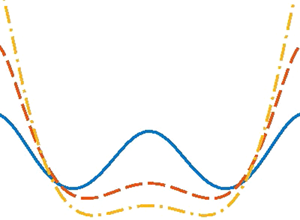
Figure 5(b,c) presents spatial profiles of the free surface  $z=\zeta _1$ and interface
  $z=-h+\zeta _2$. As
  $\epsilon$ increases, crests and troughs steepen in both the free-surface and interface profiles. Combining the results of figure 5(b,c), we find that the primary components of the surface and interface waves are out of phase, and the resonant components of the surface and interface waves have the same phase. This phase relation is identical to that found by Parau & Dias (Reference Parau and Dias2001).
3.1.3. Finite amplitude waves
We now consider the effect of upper-layer depth on finite amplitude interfacial waves. Figure 6 presents the variation in energy proportions of surface and interface waves, and all primary and resonant components in the whole wave field, with the upper-layer depth parameter  $kh$. Square symbols represent the
  $1:2$ exactly resonant case. For small upper-layer depth (
 $kh=0.597$), both the surface and interface waves carry a similar amount of energy. As the upper-layer depth increases, energy is transferred from the interface waves to the surface waves. Energy transported by the surface waves reaches a maximum (
 $71\,\%$ of total energy) near the exactly resonant value of upper-layer depth parameter (
 $kh=0.675$). As the upper-layer depth further increases, energy is transferred back from the surface waves to the interface waves. At
  $kh=0.942$, the energy carried by the surface waves is nearly equal to that carried by the interface waves. For surface waves, as
  $kh$ increases, energy carried by the primary component
  $E^{S}_{1}$ first increases and then decreases slowly, while energy transported by the resonant component
  $E^{S}_{2}$ keeps decreasing. For interface waves,
  $E^{I}_{1}$ increases while
  $E^{I}_{2}$ decreases, both progressively, with
  $kh$. Note that the wavelength of the primary component is twice that of the resonant component. Therefore, as the upper-layer depth increases, wave energy transfers from the shorter resonant component to the longer primary component for both surface and interface waves.

Figure 6. Variations of energy proportion in (a) surface and interface waves, and (b) primary and resonant components with upper-layer depth parameter  $kh$ when
  $\varDelta =0.1$ and
  $\epsilon =1.05$. The square symbols indicate
  $1:2$ exact resonance.
Figure 7(a) shows the dimensionless amplitudes of the four largest components  $|kC^{\eta _1}_{1}|$,
  $|kC^{\eta _1}_{2}|$,
  $|kC^{\eta _2}_{1}|$ and
  $|kC^{\eta _2}_{2}|$ for different values of the upper-layer depth parameter
  $kh$. The amplitude of each component changes continuously with
  $kh$. Here the superimposed square symbols indicate the
  $1:2$ exactly resonant case. The energy carried by surface waves and interface waves exhibits mirror symmetry, even though the density of the upper layer,
  $\rho _1$, is smaller than that of the lower layer,
  $\rho _2$. For almost all
  $kh$, the amplitudes of the primary and resonant components of surface waves are larger than the corresponding amplitudes of interface waves. At
  $kh=0.597$, the resonant surface component
  $|kC_{2}^{\eta _1}|$ is largest. As
  $kh$ increases, the amplitudes of the primary components of both surface and interface increase more rapidly than those of the resonant components. Hence at
  $kh=0.942$, the largest component is the primary surface component
  $|kC_{1}^{\eta _1}|$.

Figure 7. Variations in (a) wave amplitude  $|kC^{\eta _j}_{i}|$, and spatial profiles of (b) free surface
  $z=\zeta _1$ and (c) interface
  $z=-h+\zeta _2$ at
  $t=0$ s with upper-layer depth parameter
  $kh$ when
  $\varDelta =0.1$ and
  $\epsilon =1.05$. The square symbols indicate
  $1:2$ exact resonance.
Figure 7(b,c) presents spatial profiles of the free surface  $z=\zeta _1$ and interface
  $z=-h+\zeta _2$ for three different values of the upper-layer depth parameter
  $kh$. The wave heights of the free-surface and interface profiles both increase with
  $kh$. In this case, the wavelength of the primary component
  $\cos (\xi )$ is twice that of the resonant component
  $\cos (2\xi )$. Due to the energy transfer shown in figure 6(b), the shapes of the free surface and interface both tend to a single sinusoidal wave as the upper-layer depth parameter
  $kh$ increases.
Figure 8(a) displays vertical profiles of the horizontal fluid particle velocity component  $u$ at the crest of the surface wave for three different values of upper-layer depth parameter
  $kh$. In all cases, the horizontal velocity gradient exhibits a jump at the interface, with the horizontal velocity component increasing with
  $z$ in the upper layer. As the upper-layer depth parameter
  $kh$ increases, the difference in horizontal velocity component across the interface increases along with the wave heights of both surface and interface, leading to a rapid increase in fluid particle velocity near the free surface. Though the non-viscous model in this paper inevitably involves a discontinuity in the velocity profile at the interface, the foregoing qualitative findings should nevertheless be reasonable.

Figure 8. Vertical profile of the horizontal fluid particle velocity component: (a)  $u=u_{ch}+u_{sh}$ in both layers, and (b) hyperbolic cosine contribution
  $u_{ch}$ and (c) hyperbolic sine contribution
  $u_{sh}$ in the upper layer at the crest of the surface wave at
  $t=0$ s, with the upper-layer depth parameter
  $kh$ when
  $\varDelta =0.1$ and
  $\epsilon =1.05$.
For the upper fluid layer, the horizontal fluid particle velocity component  $u$ in figure 8(a) comprises a hyperbolic cosine part
  $u_{ch}$ and a hyperbolic sine part
  $u_{sh}$ (
 $u=u_{ch}+u_{sh}$) as evident in the solution expression (2.24). Figure 8(b,c) shows vertical profiles of these velocity contributions,
  $u_{ch}$ and
  $u_{sh}$, for three values of the upper-layer depth parameter
  $kh$. It can be seen that
  $u_{ch}$ tends to increase with the upper-layer depth parameter
  $kh$, whereas
  $u_{sh}$ decreases with
  $kh$. At
  $kh=0.942$, the hyperbolic sine contribution
  $u_{sh}$ is sufficiently small to be ignored. As
  $kh$ decreases,
  $u_{sh}$ becomes increasingly important compared with
  $u_{ch}$.
In general, the amplitudes of finite amplitude interfacial waves change continuously with upper-layer depth parameter  $kh$. The energy carried by surface waves with varying water depth mirrors that carried by interface waves. As the upper-layer depth increases, energy flux transfers within surface and interface waves occur from the shorter resonant component to the longer primary one.
3.2. The $1:3$ resonance

Taking  $1:3$ resonance as an example, we consider the third-harmonic resonance of steady-state interfacial waves with free-surface boundary conditions. Weakly nonlinear cases with
  $\epsilon =1.0002$ are considered, and convergent series solutions obtained in the vicinity of the exactly resonant point. Figure 9 shows the dimensionless amplitudes of the four largest components
  $|kC^{\eta _1}_{1}|$,
  $|kC^{\eta _1}_{3}|$,
  $|kC^{\eta _2}_{1}|$ and
  $|kC^{\eta _2}_{3}|$ for different values of upper-layer depth parameter
  $kh$. Here the square symbols represent
  $1:3$ exact resonance. The amplitudes of all four components increase with
  $kh$. For small
  $kh$, the surface wave resonant component
  $\cos (3\xi )$ dominates. As
  $kh$ increases, the situation alters so that the primary component
  $\cos (\xi )$ and resonant component
  $\cos (3\xi )$ of the surface wave instead become dominant.

Figure 9. Variation in wave amplitude  $|kC^{\eta _j}_{i}|$ with upper-layer depth parameter
  $kh$, when
  $\varDelta =0.1$ and
  $\epsilon =1.0002$. The superimposed square symbols indicate
  $1:3$ exact resonance.
4. Concluding remarks
We have investigated steady-state periodic interfacial gravity waves with  $1:2$ and
  $1:3$ exact- and near-harmonic resonances. The interfacial waves exist in a two-layer fluid with a free surface. A robust solution procedure based on a modification to the HAM framework has been used to remove the singularity and small divisor respectively caused by exact and near resonance. Convergent series solutions have been obtained and the continuum of steady-state interfacial waves in parameter space is established.
For interfacial waves with  $1:2$ exact resonance, as nonlinearity increases, energy carried by the primary component transfers to the resonant component within the surface waves, whereas energy carried by the resonant component transfers to the primary one within interface waves. The amplitude of the primary component is invariably larger than that of the resonant component for both surface and interface waves. And the amplitudes of surface wave components are much larger than those of the interface wave.
For finite amplitude interfacial waves with  $1:2$ near resonance, energy carried by surface and interface waves exhibits mirror symmetry as the upper-layer depth varies. For both surface and interface waves, energy transfers from the shorter resonant component to the longer primary component as the upper-layer depth increases. This explains why the spatial profiles of both free surface and interface tend to a single sinusoidal waveform as the upper layer becomes deeper. By considering vertical profiles of the horizontal fluid particle velocity component, an increasingly rapid rise in horizontal velocity is found to occur near the free surface as the upper-layer depth and wave heights of both the free surface and interface jointly increase. The analytical solutions show that the horizontal fluid particle velocity is composed of hyperbolic components, with the hyperbolic sine contribution growing in importance over the hyperbolic cosine contribution as the upper-layer depth decreases.
For weakly nonlinear interfacial waves around the  $1:3$ exact resonance point, convergent series solutions are obtained. A steady-state triad resonant system in a two-layer fluid with free surface subject to more realistic conditions will be studied in the future.
Harmonic resonance with small  $N$ does not exist for two-layer fluids with large density ratio
  $\varDelta$, as demonstrated by the resonant curves in figure 2. Without loss of generality,
  $\varDelta =0.1$ has been chosen for all cases considered in this paper to facilitate the occurrence of
  $1:2$ and
  $1:3$ resonances. In this work, the small divisors associated with near resonance for interfacial waves are removed by the HAM. It should be noted that several advanced perturbation methods (such as the multiple scales method) that work for finite amplitude waves and over long duration could also treat singularities and small divisors in an elegant, rigorous, simple way. For steeper wave groups than considered in this work, the present formulation based on potential flow theory becomes invalid as soon as viscosity and wave breaking come into play.
Funding
This work was partly supported by the National Natural Science Foundation of China (approval nos. 12072126, 51609090 and 11432009) and the State Key Laboratory of Ocean Engineering of China (approval no. 1806).
Declaration of interests
The authors report no conflict of interest.
Appendix A. Interface deformation conditions
The two kinematic interface conditions are
 \begin{equation} \frac{\partial\zeta_2}{{\partial}t}+\boldsymbol{\nabla}\phi_{1}\boldsymbol{\cdot}\boldsymbol{\nabla}\zeta_{2}-\frac{\partial\phi_{1}}{{\partial}z}=0, \quad \text{at}\ z={-}h+\zeta_{2} \end{equation}
and
 \begin{equation} \frac{\partial\zeta_2}{{\partial}t}+\boldsymbol{\nabla}\phi_{2}\boldsymbol{\cdot}\boldsymbol{\nabla}\zeta_{2}-\frac{\partial\phi_{2}}{{\partial}z}=0, \quad \text{at}\ z={-}h+\zeta_{2}. \end{equation}
The dynamic interface condition is
 \begin{equation} \rho_{1}\left(\frac{\partial\phi_{1}}{{\partial}t}+g\zeta_2+\frac{1}{2}{\left|\boldsymbol{\nabla}\phi_{1} \right|}^{2}\right)-\rho_{2}\left(\frac{\partial\phi_{2}}{{\partial}t} +g\zeta_2+\frac{1}{2}{\left|\boldsymbol{\nabla}\phi_{2}\right|}^{2}\right)=0, \quad \text{at}\ z={-}h+\zeta_{2}. \end{equation}
Given that  $\varDelta =\rho _{1}/\rho _{2}$, the interface disturbance
  $\zeta _2$ is obtained by solving equation (A3) to give
 \begin{equation} \zeta_{2}=\frac{1}{g(1-\varDelta)}\left[\varDelta\left(\frac{\partial\phi_{1}}{\partial t}+\frac{1}{2}{\left|\boldsymbol{\nabla}\phi_{1}\right|}^{2}\right)-\left(\frac{\partial\phi_{2}}{\partial t}+\frac{1}{2}{\left|\boldsymbol{\nabla}\phi_{2}\right|}^{2}\right)\right], \quad \text{at}\ z={-}h+\zeta_{2}. \end{equation}
 Carrying out partial differentiation of (A4) with respect to  $x$,
$x$,  $y$ and
  $t$, and substituting into (A1)–(A2),
  $\zeta _2$ is then eliminated to give
 \begin{gather} \frac{\partial^{2}\phi_{2}}{\partial t^{2}}+g(1-\varDelta)\frac{\partial\phi_{2}}{\partial z}-\varDelta\frac{\partial^{2}\phi_{1}}{\partial t^{2}}+\frac{\partial ({\left|\boldsymbol{\nabla}\phi_{2}\right|}^{2})} {\partial t}-\varDelta\frac{\partial \left(\frac{1}{2}{\left|\boldsymbol{\nabla}\phi_{1}\right|}^{2}\right)}{\partial t}+\boldsymbol{\nabla}\phi_{2}\boldsymbol{\cdot}\boldsymbol{\nabla} \left(\frac{1}{2}{\left|\boldsymbol{\nabla}\phi_{2}\right|}^{2}\right)\nonumber\\ -\varDelta\boldsymbol{\nabla}\phi_{2}\boldsymbol{\cdot}\boldsymbol{\nabla}\left(\frac{\partial\phi_{1}}{\partial t}+\frac{1}{2}{\left|\boldsymbol{\nabla}\phi_{1}\right|}^{2}\right)=0, \quad \text{at}\ z={-}h+\zeta_{2} \end{gather}
and
 \begin{gather} \frac{\partial^{2}\phi_{2}}{\partial t^{2}}+g(1-\varDelta)\frac{\partial\phi_{1}}{\partial z}-\varDelta\frac{\partial^{2}\phi_{1}}{\partial t^{2}}+\frac{\partial \left(\frac{1}{2}{\left|\boldsymbol{\nabla}\phi_{2}\right|}^{2}\right)}{\partial t}-\varDelta\frac{\partial ({\left|\boldsymbol{\nabla}\phi_{1}\right|}^{2})} {\partial t}-\varDelta\boldsymbol{\nabla}\phi_{1}\boldsymbol{\cdot}\boldsymbol{\nabla} \left(\frac{1}{2}{\left|\boldsymbol{\nabla}\phi_{1}\right|}^{2}\right)\nonumber\\ +\boldsymbol{\nabla}\phi_{1}\boldsymbol{\cdot}\boldsymbol{\nabla} \left(\frac{\partial\phi_{2}}{\partial t}+\frac{1}{2}{\left|\boldsymbol{\nabla}\phi_{2}\right|}^{2}\right)=0, \quad \text{at}\ z={-}h+\zeta_{2}. \end{gather}
Subtracting (A6) from (A5), we obtain
 \begin{gather} g(1-\varDelta)\frac{\partial(\phi_{2}-\phi_{1})}{\partial z}+\frac{\partial \left(\frac{1}{2}{\left|\boldsymbol{\nabla}\phi_{2}\right|}^{2}\right)}{\partial t}+\boldsymbol{\nabla}\phi_{2}\boldsymbol{\cdot}\boldsymbol{\nabla} \left(\frac{1}{2}{\left|\boldsymbol{\nabla}\phi_{2}\right|}^{2}\right) -\boldsymbol{\nabla}\phi_{1}\boldsymbol{\cdot}\boldsymbol{\nabla} \left(\frac{\partial\phi_{2}}{\partial t}+\frac{1}{2}{\left|\boldsymbol{\nabla}\phi_{2}\right|}^{2}\right)\nonumber\\ +\varDelta\left[\frac{\partial \left(\frac{1}{2}{\left|\boldsymbol{\nabla}\phi_{1}\right|}^{2}\right)}{\partial t}+\boldsymbol{\nabla}\phi_{1}\boldsymbol{\cdot}\boldsymbol{\nabla} \left(\frac{1}{2}{\left|\boldsymbol{\nabla}\phi_{1}\right|}^{2}\right)\right.\nonumber\\ \left. -\boldsymbol{\nabla}\phi_{2}\boldsymbol{\cdot}\boldsymbol{\nabla} \left(\frac{\partial\phi_{1}}{\partial t}+\frac{1}{2}{\left|\boldsymbol{\nabla}\phi_{1}\right|}^{2}\right)\right]=0, \quad \text{at}\ z={-}h+\zeta_{2}. \end{gather}
Subsequent derivation is then based on the kinematic interface conditions (A5), (A7) and dynamic interface condition (A4). Note that (A5) is (2.5), (A7) is (2.6) and (A4) is (2.7).
Appendix B. High-order deformation equations in the HAM
Substituting the series (2.37a,b)–(2.38a,b) into the zeroth-order deformation equations (2.32)–(2.36), and then equating like-powers of  $q$, the following five linear equations (called high-order deformation equations) are obtained:
 \begin{gather} {\mathcal{L}}_{1}[\varphi_{m,1}]|_{z=0}=c_{0}\varDelta_{m-1,1}^{\varphi}+\chi_{m}(S_{m-1,1}-\bar{S}_{m,1}),\quad m\geq1, \end{gather}
 \begin{gather} {\mathcal{L}}_{i+1}[\varphi_{m,1},\varphi_{m,2}]|_{z={-}h}=c_{0}\varDelta_{m-1,i}^{\varphi}+\chi_{m}(S_{m-1,i}-\bar{S}_{m,i}),\quad i=2,3,\quad m\geq1, \end{gather}
 \begin{gather} \eta_{m,i}=c_{0}\varDelta_{m-1,i}^{\eta}+\chi_{m}\eta_{m-1,i},\quad i=1,2,\quad m\geq1, \end{gather}
where
 \begin{gather} \varDelta_{m,1}^{\varphi}=\sigma^2\bar{\phi}_{m}^{2,1,1}+g\bar{\phi}_{z,m}^{0,1,1} +\varLambda_{m,1}^{1,1,1}-2\sigma\varGamma_{m,1}^{1,1}, \end{gather}
 \begin{gather} \varDelta_{m,2}^{\varphi}=\sigma^2\bar{\phi}_{m}^{2,2,2}+g(1-\varDelta)\bar{\phi}_{z,m}^{0,2,2} -\varDelta\sigma^2\bar{\phi}_{m}^{2,1,2}+\varLambda_{m,1}^{2,2,2}\nonumber\\ -2\sigma\varGamma_{m,1}^{2,2}+\varDelta(\sigma\varGamma_{m,1}^{1,2}-\varLambda_{m,2}^{2,1,2}-\varLambda_{m,1}^{2,1,2}), \end{gather}
 \begin{gather} \varDelta_{m,3}^{\varphi}=g(1-\varDelta)(\bar{\phi}_{z,m}^{0,2,2} -\bar{\phi}_{z,m}^{0,1,2})-\sigma\varGamma_{m,1}^{2,2} +\varLambda_{m,1}^{2,2,2}-\varLambda_{m,2}^{1,2,2}-\varLambda_{m,1}^{1,2,2}\nonumber\\ +\varDelta(\varLambda_{m,1}^{1,1,2}-\varLambda_{m,2}^{2,1,2}-\varLambda_{m,1}^{2,1,2}-\sigma\varGamma_{m,1}^{1,2}), \end{gather}
 \begin{gather} \varDelta_{m,1}^{\eta}=\eta_{m,1}-\frac{1}{g}(\sigma\bar{\phi}_{m}^{1,1,1}-\varGamma_{m,0}^{1,1}), \end{gather}
 \begin{gather} \varDelta_{m,2}^{\eta}=\eta_{m,2}+\frac{1}{g(1-\varDelta)}[\varGamma_{m,0}^{2,2}-\sigma\bar{\phi}_{m}^{1,2,2} +\varDelta(\sigma\bar{\phi}_{m}^{1,1,2}-\varGamma_{m,0}^{1,2})], \end{gather}
in which
 \begin{gather} \varGamma_{m,0}^{\bar{k},p}=\sum_{n=0}^{m}\left(\frac{k^{2}}{2}\bar{\phi}_{n}^{1,\bar{k},p}\bar{\phi}_{m-n}^{1,\bar{k},p} +\frac{1}{2}\bar{\phi}_{z,n}^{0,\bar{k},p}\bar{\phi}_{z,m-n}^{0,\bar{k},p}\right),\quad \bar{k},p=1,2, \end{gather}
 \begin{gather} \varGamma_{m,1}^{\bar{k},p}=\sum_{n=0}^{m}[k^{2}\bar{\phi}_{n}^{1,\bar{k},p} \bar{\phi}_{m-n}^{2,\bar{k},p}+\bar{\phi}_{z,n}^{0,\bar{k},p}\bar{\phi}_{z,m-n}^{1,\bar{k},p}],\quad \bar{k},p=1,2, \end{gather}
 \begin{gather} \varGamma_{m,3}^{\bar{k},p}=\sum_{n=0}^{m}[k^{2}\bar{\phi}_{n}^{1,\bar{k},p}\bar{\phi}_{z,m-n}^{1,\bar{k},p} +\bar{\phi}_{z,n}^{0,\bar{k},p}\bar{\phi}_{zz,m-n}^{0,\bar{k},p}],\quad \bar{k},p=1,2, \end{gather}
 \begin{gather} \varLambda_{m,1}^{i,j,p}=\sum_{n=0}^{m}[k^{2}\bar{\phi}_{n}^{1,i,p}\varGamma_{m-n,1}^{j,p} +\bar{\phi}_{z,n}^{0,i,p}\varGamma_{m-n,3}^{j,p}],\quad i,j,p=1,2, \end{gather}
 \begin{gather} \varLambda_{m,2}^{i,j,p}={-}\sigma\sum_{n=0}^{m}[k^{2}\bar{\phi}_{n}^{1,i,p}\bar{\phi}_{m-n}^{2,0,j,p}+\bar{\phi}_{z,n}^{0,i,p}\bar{\phi}_{z,m-n}^{1,j,p}],\quad i,j,p=1,2, \end{gather}
 \begin{gather} \mu_{m,n,p}=\left\{ \begin{array}{@{}cc} \eta_{n,p}, & m=1,\quad n\geq1,\\ \displaystyle\sum_{i=m-1}^{n-1}\mu_{m-1,i,p}\eta_{n-i,p}, & m\geq2,\quad n\geq m, \end{array} \right. \end{gather}
 \begin{gather} \psi_{i,\bar{k},1}^{n,m}=\frac{\partial^{i}}{\partial\xi^{i}}\left.\left(\frac{1}{m!}{\frac{\partial^{m}\varphi_{n,\bar{k}}}{\partial z^{m}}}\right|_{z=0}\right),\quad \bar{k}=1,2, \end{gather}
 \begin{gather} \psi_{i,\bar{k},2}^{n,m}=\frac{\partial^{i}}{\partial\xi^{i}}\left.\left(\frac{1}{m!}{\frac{\partial^{m}\varphi_{n,\bar{k}}}{\partial z^{m}}}\right|_{z={-}h}\right),\quad \bar{k}=1,2, \end{gather}
 \begin{gather} \beta_{i,\bar{k},p}^{n,m}=\left\{ \begin{array}{@{}cc} \psi_{i,\bar{k},p}^{n,0}, & m=0,\\ \displaystyle\sum_{s=1}^{m}\psi_{i,\bar{k},p}^{n,s}\mu_{s,m,p}, & m\geq1, \end{array} \right. \end{gather}
 \begin{gather} \gamma_{i,\bar{k},p}^{n,m}= \left\{ \begin{array}{@{}cc} \psi_{i,\bar{k},p}^{n,1}, & m=0,\\ \sum_{s=1}^{m}(s+1)\psi_{i,\bar{k},p}^{n,s+1}\mu_{s,m,p}, & m\geq1, \end{array} \right. \end{gather}
 \begin{gather} \delta_{i,\bar{k},p}^{n,m}=\left\{ \begin{array}{@{}cc} 2\psi_{i,\bar{k},p}^{n,2}, & m=0,\\ \displaystyle\sum_{s=1}^{m}(s+1)(s+2)\psi_{i,\bar{k},p}^{n,s+2}\mu_{s,m,p}, & m\geq1, \end{array} \right. \end{gather}
 \begin{gather} \bar{\phi}_{n}^{i,\bar{k},p}=\sum_{m=0}^{n}\beta_{i,\bar{k},p}^{n-m,m},\quad \bar{\phi}_{z,n}^{i,\bar{k},p}=\sum_{m=0}^{n}\gamma_{i,\bar{k},p}^{n-m,m},\quad \bar{\phi}_{zz,n}^{i,\bar{k},p}=\sum_{m=0}^{n}\delta_{i,\bar{k},p}^{n-m,m}. \end{gather}
Expressions for  ${\mathcal {L}}_{i}$,
  $S_{m-1,i}$ and
  $\bar {S}_{m,i}$ are given in § 2.3.2.


