


1. Introduction
The Reynolds number is one of the most fundamental dimensionless numbers in fluid mechanics. In the literature it is often referred to as the ratio of inertial to viscous forces, both of which are key ingredients of Newtonian fluid mechanics. The ratio can be defined locally at any given position  ${{\boldsymbol {x}}}$ and time
  $t$. In this paper this ratio is called the local Reynolds number and denoted as
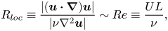
  $R_{loc}$, i.e.
 \begin{equation} R_ {loc} \equiv \frac {| ({{\boldsymbol{u}}} \boldsymbol{\cdot} \boldsymbol{\nabla}) {{\boldsymbol{u}}}|}{|\nu \nabla^{2} {{\boldsymbol{u}}}|}, \end{equation}
where  ${{\boldsymbol {u}}}={{\boldsymbol {u}}} ({{\boldsymbol {x}}},t)$ is the fluid velocity at the position
  ${{\boldsymbol {x}}}$ and time
  $t$,
$t$,  $\nu \equiv \mu /\rho$ is the kinematic viscosity, and
  $\mu$ and
  $\rho$ are the fluid viscosity and density, respectively. In the following, we may omit writing
  $({{\boldsymbol {x}}},t)$. (Note: In some of the literature, the word ‘inertial force’ is used to mean
 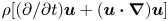 $\rho [(\partial /\partial t){{\boldsymbol {u}}}+ ({{\boldsymbol {u}}} \boldsymbol {\cdot } \boldsymbol {\nabla }) {{\boldsymbol {u}}}]$, and the term
  $\rho ({{\boldsymbol {u}}} \boldsymbol {\cdot } \boldsymbol {\nabla }) {{\boldsymbol {u}}}$ is called the advective term. In this paper, the word ‘inertial force’ is used to mean
  $\rho ({{\boldsymbol {u}}} \boldsymbol {\cdot } \boldsymbol {\nabla }) {{\boldsymbol {u}}}$.)
Let  $L$ and
  $U$ be representative length and velocity scales characterizing the flow field in a global sense, and let the (global) Reynolds number
  $Re$ be defined by
 \begin{equation} Re \equiv \frac{UL}{\nu}. \end{equation}
Here,  $L$ and
  $U$ are independent of the position, so that
  $Re$ is too. For example, in the context of homogeneous turbulence, one may put
  $L$ and
  $U$ to be respectively the characteristic length and velocity scales of energy-containing eddies. Equation (1.2) is one of the most commonly used definitions of Reynolds number.
The use of simple estimates  ${{\boldsymbol {u}}} \sim U$ and
  $\boldsymbol {\nabla } \sim 1/L$ yields
 \begin{equation} ({{\boldsymbol{u}}} \boldsymbol{\cdot} \boldsymbol{\nabla}) {{\boldsymbol{u}}} \sim \frac{U^{2}}{L}, \quad \nu \nabla^{2} {{\boldsymbol{u}}} \sim \nu \frac{U}{L^{2}}, \end{equation}
so that one might think
 \begin{equation} R_ {loc} \equiv \frac {| ({{\boldsymbol{u}}} \boldsymbol{\cdot} \boldsymbol{\nabla}) {{\boldsymbol{u}}}|}{|\nu \nabla^{2} {{\boldsymbol{u}}}|} \sim Re\equiv \frac{UL}{\nu}, \end{equation}
where the symbol ‘ $\sim$’ means equality in a certain appropriate sense of the order of magnitude. However, as is well known, (1.4) is not necessarily correct, and the distribution of the ratio
  $R_{loc}$ is in general not uniform and indeed can be very non-uniform.
In the case of certain classes of laminar flows, such as slow flows past a body at small but finite  $Re$ and flows past a solid wall of simple geometry at high
  $Re$, it is not difficult to get some idea of the distribution of the ratio
  $R_{loc}$ analytically. By contrast, for complex flows, in particular turbulent flows, it is difficult to get analytically information about
  $R_{loc}$. Little is known about the distribution of
  $R_{loc}$ in turbulent flows, as compared with laminar flows.
In general, flows at high  $Re$ are turbulent, and such flows exhibit strong non-uniformity in the distributions of flow characteristics such as the velocity fluctuation, velocity gradients, etc. The fluctuations at small scales are strong in some regions (called active regions), while they are weak in others (called calm or non-active regions); see, e.g. figures 1 and 4 in Ishihara, Gotoh & Kaneda (Reference Ishihara, Gotoh and Kaneda2009). Even if the flow is statistically homogeneous, the spatial distribution of ‘activeness’ is in general not uniform; thus, the distribution of the ratio
  $R_{loc}$ may not be uniform, in accordance with the non-uniformity of the activeness. Then, one can ask, for example, the following questions: ‘Is the estimate
  $R_{loc} \sim Re$, i.e. (1.4), acceptable?’; and if not, ‘How large or small is the difference between
  $R_{loc}$ and
  $Re$?’; ‘How is the influence of activeness on the statistics of the inertial and viscous forces, and on the ratio
  $R_{loc}$?’; and so on. (Regarding the first two questions, it may be worthwhile to note that Orszag (Reference Orszag1977) gave the estimate
  $R_{loc} =O(Re^{1/4})$; see § 4.)
Although it is difficult to answer these questions analytically, it is at least in principle not difficult to estimate  $R_{loc}$ in direct numerical simulation (DNS) of the flow field. Thanks to developments in computation, it is now possible for us to simulate turbulent flows at considerably high Reynolds numbers, and estimate
  $R_{loc}$. In this study we consider the statistics of
  $R_{loc}$ on the basis of the data of a series of DNS of forced turbulence of an incompressible fluid in a periodic box, so-called box turbulence, with the Taylor-microscale Reynolds number
  $R_\lambda$ up to approximately 1100.
In order to get some idea of the influence of the activeness on the statistics of  $R_{loc}$, particular attention is paid in this study to joint probability distribution functions (p.d.f.s)
  $P(X,Y)$, where
  $X=X({{\boldsymbol {x}}},t)$ is a measure representing the activeness at
  $({{\boldsymbol {x}}},t)$, and
  $Y=Y({{\boldsymbol {x}}},t)$ is the magnitude of the inertial or viscous force under appropriate normalization, or the ratio
  $R_{loc}({{\boldsymbol {x}}},t)$. Among measures that can represent activeness, we use here the normalised squared vorticity
  ${{\omega ^{2}/\langle \omega ^{2} \rangle }}$ or the normalised local energy dissipation rate per unit mass
  ${{\epsilon /\langle \epsilon \rangle }}$, where
  $\omega ^{2}\equiv |\boldsymbol {\nabla } \times {{{\boldsymbol {u}}}}|^{2}$,
  $\epsilon \equiv 2 \nu s^{2}$,
  $s^{2}\equiv S_{ij}S_{ij}$, and
  $S_{ij}\equiv (\partial u_i/\partial x_j+\partial u_j/\partial x_i)/2$. In the following,
  $\epsilon$ is called simply the energy dissipation rate. The brackets
  $\langle \cdots \rangle$ denote the spatial average over the space, and the summation convention is used for repeated indices. The present work stemmed from a study of the small-scale structure of turbulence on the basis of high-resolution DNS of box turbulence (Kaneda & Morishita Reference Kaneda and Morishita2013).
(Note: In our study, the local Reynolds number  $R_{loc}$ is defined by (1.1). It is different from another local Reynolds number
  $R_r$ defined by
 \begin{equation} R_r \equiv \frac{V_r r}{\nu}, \end{equation}
where  $V_r$ is the order of magnitude of the turbulent velocity variation over distances of the order of
  $r$ at
  $({{{\boldsymbol {x}}}},t)$ (e.g. Kolmogorov Reference Kolmogorov1962; Monin & Yaglom Reference Monin and Yaglom1975; Landau & Lifshitz Reference Landau and Lifshitz1987). In the theory of Kolmogorov and Oboukhov (Kolmogorov Reference Kolmogorov1962),
  $V_r$ is given by
  $V_r=(\epsilon _r r)^{1/3}$, where
  $\epsilon _r$ is the average of the energy dissipation rate per unit mass over the sphere of radius
  $r$ centred at the position
  ${{\boldsymbol {x}}}$. Here we assume that
  $r \ll L$, i.e.
  $r$ is in the small-scale range. The idea that
  $R_r$ is different from
  $Re$ and non-uniformly distributed is well known in studies of small-scale intermittency.
One should distinguish  $R_r$ and
  $R_{loc}$ from each other. While
  $R_{loc}$ depends only on the position and time
  $({{{\boldsymbol {x}}}}, t)$,
  $R_r$ depends not only on
  $({{{\boldsymbol {x}}}},t)$ but also on the scale
  $r$. In contrast to
  $R_r$, the advective term and
  $R_{loc}$ are not invariant under Galilean transformation. This implies that
  $R_{loc}$ is not free from the so-called random sweeping effects by large eddies. This suggests that the statistics of
  $R_{loc}$ can be significantly influenced not only by the small-scale statistics, but also the statistics of large-scale energy-containing eddies, which are in general non-universal. Therefore, it would not be surprising if the statistics of
  $R_{loc}$ are fundamentally different from those of
  $R_r$. The knowledge of the statistics of only
  $V_r$, or
  $\epsilon _r$ if
  $V_r$ is given by
  $V_r=(\epsilon _r r)^{1/3}$ at small scales, is not sufficient to fix the statistics of
  $R_{loc}$, in contrast to
  $R_r$, because the large-scale statistics may have significant influence on
  $R_{loc}$.)
2. Direct numerical simulation method and run conditions
The results presented below are based on the analysis of data of DNS of turbulent flow of an incompressible fluid obeying the Navier–Stokes (NS) equation in a periodic box. The fluid is forced at only low wavenumber modes by using negative viscosity. The total energy per unit mass  $\langle {{\boldsymbol {u}}}\boldsymbol {\cdot }{{\boldsymbol {u}}} \rangle /2$ is maintained at an almost time-independent constant
  $\approx 0.5$, and there is no mean flow, i.e.
  $\langle {{\boldsymbol {u}}}\rangle =\textbf {0}$. The DNS is based on a Runge–Kutta method for time advancing, and an alias-free spectral method. For some details of the DNS method and numerical results, readers may refer to Ishihara et al. (Reference Ishihara, Morishita, Yokokawa, Uno and Kaneda2016) and Ishihara et al. (Reference Ishihara, Kaneda, Morishita, Yokokawa and Uno2020), which respectively show the energy spectrum and the second-order structure functions.
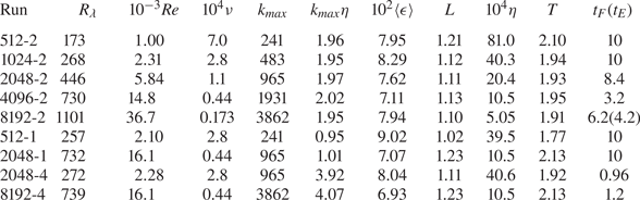
Some DNS parameters are given in table 1, where  $R_\lambda$ is the Taylor-microscale Reynolds number,
  $Re=u'L/\nu$,
  $3 u'^{2} =\langle {{\boldsymbol {u}}}\boldsymbol {\cdot }{{\boldsymbol {u}}} \rangle$,
  $k_{ max}$ is the maximum wavenumber retained in the DNS, the minimum wavenumber is 1,
  $\eta$ is the Kolmogorov microscale given by
  $\eta =(\nu ^{3}/\langle \epsilon \rangle )^{1/4}$, and
  $L$ is the characteristic length scale of the energy-containing eddies defined by
 \begin{equation} L \equiv \frac{\rm \pi}{2u'^{2}} \int_0^{k_{ max}} \frac{E(k)}{k}\,\textrm{d}k, \end{equation}
in which  $E(k)$ is the energy spectrum, satisfying
  $3u'^{2}/2=\int _0^{k_{ max}} E(k) \textrm {d} k$, and
  $T$ is the eddy turnover time given by
  $T=L/u'$.
Table 1. Direct numerical simulation parameters and turbulence characteristics at time  $t=t_{F}$.
The numbers such as  $4096$ and
  $2$ in the run names stand for the number
  $N$ of the grid points in each direction of the Cartesian coordinates and the resolution
  $k_{ max} \eta$ at time
  $t_{F}$; ‘run
  $m$–
$m$– $n$’, except run 8192-2, was advanced in time with
  $N=m$ and
  $k_{ max} \eta \approx n$ until time at least
  $t_{F}$. Run 8192-2 was first advanced in time with
  $k_{ max} \eta \approx 1$ and
  $N=4096$ until the time
  $t=t_{E}$ before the setting to
  $N=8192$ and
  $k_{ max} \eta \approx 2$. The data of runs 512-2, 1024-2, 2048-2, 512-1 and 2048-1 are from the runs used in Ishihara et al. (Reference Ishihara, Kaneda, Yokokawa, Itakura and Uno2007). The initial fields of runs 4096-2 (8192-2, 8192-4) and 2048-4, were respectively given by the fields at the final time step of runs 2048-1 and 1024-2 in Ishihara et al. (Reference Ishihara, Kaneda, Yokokawa, Itakura and Uno2007). The computation used double-precision arithmetic.
3. Influence of squared vorticity  $\omega ^{2}$

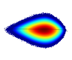
Figure 1(a–c) shows the pre-multiplied joint p.d.f.s  $XYP(X,Y)$ for
  $X \equiv \omega ^{2}/\langle \omega ^{2} \rangle$ and
  $Y=|({{\boldsymbol {u}}} \boldsymbol {\cdot } \boldsymbol {\nabla }) {{\boldsymbol {u}}}|/(u'u_\eta /\eta )$,
 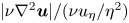 $| \nu \nabla ^{2} {{\boldsymbol {u}}}|/(\nu u_\eta /\eta ^{2})$, and
  $R_{loc}$, respectively, where
  $u_\eta$ is the Kolmogorov microscale velocity given by
  $u_\eta =(\langle \epsilon \rangle \nu )^{1/4}$. The DNS data presented in this paper are from those at the instant
  $t=t_{F}$, and unless otherwise stated they are from run 8192-2.
Figure 1. Pre-multiplied joint p.d.f.s  $XYP(X,Y)$ for
  $X=\omega ^{2}/\langle \omega ^{2}\rangle$, and (a)
  $Y=|({{\boldsymbol {u}}}\boldsymbol {\cdot }\boldsymbol {\nabla }){{\boldsymbol {u}}}|/(u'u_\eta /\eta )$, (b)
  $Y=|\nu \nabla ^{2} {{\boldsymbol {u}}}|/(\nu u_\eta /\eta ^{2})$ and (c)
  $Y=R_{loc}$ in run 8192-2. (d–f) The same as (a–c), respectively, but for the random field. Vertical colour bars indicate the mapping of
  $XYP(X,Y)$ values into the colour map. Dashed lines show the conditional averages
  $\langle Y|X \rangle$ for a given
  $X=\omega ^{2}/\langle \omega ^{2}\rangle$. The solid lines in (a,b) and the dotted line in (b) respectively show
  $Y = X^{1/2}$ and
  $Y = X^{3/4}$ (see (4.16a,b)).
The dashed lines show the conditional averages of  $Y$ for a given
  $X=\omega ^{2}/\langle \omega ^{2} \rangle$. These figures are to be compared with figure 1(d–f), which plot the same statistics as figure 1(a–c), respectively, but for an artificial random structureless field
  ${{\boldsymbol {u}}}_R$ generated by randomizing the phases of the Fourier velocity components of the DNS field as
 \begin{equation} \hat{{\boldsymbol{u}}}_R({{\boldsymbol{k}}})= \left( \hat{{\boldsymbol{u}}}({{{\boldsymbol{k}}}})\cos \phi({{{\boldsymbol{k}}}} )+ \frac{{{{\boldsymbol{k}}}}}{k} \times \hat{{\boldsymbol{u}}}({{{\boldsymbol{k}}}}) \sin \phi({{{\boldsymbol{k}}}}) \right) e^{i \theta({{{\boldsymbol{k}}}}) }, \end{equation}
where  ${{\boldsymbol {k}}}$ is the wave vector,
  $\hat {{\boldsymbol {u}}}_R({{\boldsymbol {k}}})$ and
  $\hat {{\boldsymbol {u}}}({{\boldsymbol {k}}})$ are respectively the Fourier transforms of
  ${{\boldsymbol {u}}}_R({{\boldsymbol {x}}})$ and
  ${{\boldsymbol {u}}}({{\boldsymbol {x}}})$,
  $\hat {{\boldsymbol {u}}}_R({{\boldsymbol {k}}})$ satisfies the reality condition of
  ${{\boldsymbol {u}}}_R({{\boldsymbol {x}}})$,
  $\theta ({{{\boldsymbol {k}}}})$ and
  $\phi ({{{\boldsymbol {k}}}})$ are random numbers distributed statistically uniformly over the range
  $[0, 2{\rm \pi} )$, and
  $( \theta ({{{\boldsymbol {k}}}}), \phi ({{{\boldsymbol {k}}}}), \theta ({{{\boldsymbol {k}}}'}), \phi ({{{\boldsymbol {k}}}'}) )$ are statistically independent from each other provided that
  ${{{\boldsymbol {k}}}}\ne {{{\boldsymbol {k}}}}'$ and
  ${{\boldsymbol {k}}}\ne -{{{\boldsymbol {k}}}}'$. Note that
  $\hat {{\boldsymbol {u}}}_R({{\boldsymbol {k}}}) \boldsymbol {\cdot } {{{\boldsymbol {k}}}}= \hat {{\boldsymbol {u}}}({{\boldsymbol {k}}}) \boldsymbol {\cdot } {{{\boldsymbol {k}}}}=\textbf {0}$, and
  $|\hat {{\boldsymbol {u}}}_R({{\boldsymbol {k}}})|=|\hat {{\boldsymbol {u}}}({{\boldsymbol {k}}})|$ for any
  ${{{\boldsymbol {k}}}}$. Here
  $u', u_\eta$ and
  $\eta$ are the same in DNS and random fields.
3.1. Statistics of the inertial force
With regard to the inertial force per unit mass, the normalised averages  $\langle |({{\boldsymbol {u}}} \boldsymbol {\cdot } \boldsymbol {\nabla }) {{\boldsymbol {u}}}|\rangle /(u' u_\eta /\eta )$ over the fundamental periodic box are 0.697 in the DNS and 0.815 in the random field, respectively. Thus, the average is smaller in the NS field than in the random structureless field. Here the field obeying the NS equation is called the NS field. This smallness in the NS field is consistent with the phenomenon known as the depression of nonlinearity in the sense that a moment in the NS field is smaller than its random counterpart; averages such as
  $\langle |{{{\boldsymbol {u}}}}\times {\boldsymbol \omega }|^{2}\rangle$ and
  $\langle | ({{{\boldsymbol {u}}}}\boldsymbol {\cdot } \boldsymbol {\nabla } ){{{\boldsymbol {u}}}} - (1/\rho )\boldsymbol {\nabla } p|^{2} \rangle$ are known to be smaller than their Gaussian counterparts, where
  $p$ is the pressure; see Kraichnan & Panda (Reference Kraichnan and Panda1988), Chen et al. (Reference Chen, Herring, Kerr and Kraichnan1989), She, Jackson & Orszag (Reference She, Jackson and Orszag1991), Tsinober (Reference Tsinober2009), and the references cited therein. (However, it is to be noted that the smallness of a moment, say
  $\langle |f| \rangle$ does not necessarily mean the smallness of
  $\langle |f|^{2} \rangle$ as compared with its random counterpart. In fact, as seen below, the average
  $\langle |f| \rangle$ for
  $f$=viscous term is smaller in the NS field than in the random field, while Parseval's identity implies that
  $\langle |f|^{2} \rangle$ in the NS is the same as that in the random field, provided that the energy spectra in the two fields are the same as in the case given by (3.1).)
Comparison of figure 1(a,d) shows that the depression of the conditional average  $\langle |({{\boldsymbol {u}}} \boldsymbol {\cdot } \boldsymbol {\nabla }){{\boldsymbol {u}}} |{{\big {\vert }}}X \rangle$ for a given
  $X \equiv {{\omega ^{2}/\langle \omega ^{2} \rangle }}$ occurs only for small
  $X$ (e.g.
  $X< X_i$) but not for larger X, where
  $X_i \approx 10^{-1}$. Figure 1(a) shows that
  $|({{\boldsymbol {u}}} \boldsymbol {\cdot } \boldsymbol {\nabla }) {{\boldsymbol {u}}}|$ and
  $X={{\omega ^{2}/\langle \omega ^{2} \rangle }}$ in DNS are not statistically independent of each other, but correlated at large
  $X$, where the conditional average sharply increases with
  $X$ in the DNS field. The increase in the DNS field is much faster than that in the random field (see figure 1d). According to figure 1(a), the former is approximately given by
 \begin{equation} \langle |({{\boldsymbol{u}}} \boldsymbol{\cdot} \boldsymbol{\nabla}) {{\boldsymbol{u}}}| {{\big{\vert}}}X\rangle \propto X^{\alpha} =\left(\frac{\omega^{2}}{\langle\omega^{2} \rangle} \right) ^{\alpha}, \quad \alpha \approx \frac{1}{2}, \end{equation}
for large  $X$ (e.g.
  $X>X_I$), where
  $X_I \approx 1$.
Note that the NS equation is invariant under any Galilean transformation, while the term  $({{\boldsymbol {u}}} \boldsymbol {\cdot } \boldsymbol {\nabla }) {{\boldsymbol {u}}}$ is not, as noted in the introduction. Its value depends on the choice of the frame, i.e. the value measured in one frame is in general different from that in a different moving frame. In the DNS used in this paper,
  $\langle {{\boldsymbol {u}}}\rangle =\textbf {0}$. Therefore, the values presented in this paper are to be understood to be those measured in the frame in which the mean flow is zero, and
  $\langle {{\boldsymbol {u}}}\boldsymbol {\cdot } {{\boldsymbol {u}}}\rangle =3u'^{2}$.
3.2. Statistics of the viscous force
Regarding the viscous force, the normalised averages  $\langle | \nu \nabla ^{2} {{\boldsymbol {u}}} | \rangle /(\nu u_\eta /\eta ^{2})$ over the fundamental periodic box are 0.280 and 0.419 in DNS and random fields, respectively. Thus, the average is again smaller in the NS field than in the random field.
It is remarkable that the pre-multiplied joint p.d.f. in figure 1(b) is similar to the one in figure 1(a). The comparison of figures 1(b) and 1(e) shows that, just like  $\langle |({{\boldsymbol {u}}} \boldsymbol {\cdot } \boldsymbol {\nabla }){{\boldsymbol {u}}} |{{\big {\vert }}}X \rangle$,
  $\langle | \nu \nabla ^{2} {{\boldsymbol {u}}} |{{\big {\vert }}}X \rangle$ is also smaller in the DNS field than in the random field for small
  $X$ (e.g.
  $X< X_v$), where
  $X_v \approx 1$, but not for larger
  $x$. That is, depression or smallness of
  $\langle | \nu \nabla ^{2} {{\boldsymbol {u}}} |{{\big {\vert }}}X \rangle$ for a given
  $X={{\omega ^{2}/\langle \omega ^{2} \rangle }}$ in the DNS field compared with the random field occurs only for small
  $X$. Figure 1(b) shows that
  $| \nu \nabla ^{2} {{\boldsymbol {u}}}|$ and
  $X={{\omega ^{2}/\langle \omega ^{2} \rangle }}$ in DNS are not statistically independent of each other but correlated at large
  $X$, where the conditional average sharply increases with
  $X$ in DNS, in contrast to the random field shown in figure 1(e). As in figure 1(b), the increase is approximately given by
 \begin{equation} \langle |\nu \nabla^{2} {{\boldsymbol{u}}} | {{\big{\vert}}}X \rangle \propto X^{\alpha}, \quad \alpha \approx \tfrac{1}{2}, \end{equation}
for large  $X$ (e.g.
  $X>X_V$), where
  $X_V \approx X_I \approx 1$.
3.3. Statistics of the local Reynolds number $R_{loc}$

For the local Reynolds numbers, the averages  $\langle R_{loc} \rangle$ over the fundamental periodic box are 67.2 and 41.8 in the DNS and the random fields, respectively. Thus, the average
  $\langle R_{loc} \rangle$ is larger in the NS field. It is observed that
  $\langle R_{loc}| X \rangle$ in figure 1(c) is almost independent of
  $X$ in the DNS field, in contrast to the random field (figure 1f). The independence of the former is consistent with the similarity between figures 1(a) and 1(b) noted above, and implies that there is a certain mechanism in the NS dynamics, which suppresses an increase in
  $R_{loc}$ with
  $X$ that is observed at large
  $X$ in figure 1(f) for the random field.
The comparison of figures 1(d) and 1(e) suggests that in the random field, the dependence of conditional average  $\langle | \nu \nabla ^{2} {{\boldsymbol {u}}} |{{\big {\vert }}}X \rangle$ on
  $X$ at large
  $X$ is considerably weaker than that of
  $\langle |({{\boldsymbol {u}}} \boldsymbol {\cdot } \boldsymbol {\nabla }) {{\boldsymbol {u}}}| {{\big {\vert }}}X \rangle$, while in the DNS field, they are similar; both of them increase sharply with
  $X$ at large
  $X$. In this sense, the difference between DNS and random fields is larger in the viscous force than in the inertial force. The enhancement of viscous force implies the suppression of
  $R_{loc}$. Figure 1(b,e) shows that the conditional average
  $\langle | \nu \nabla ^{2} {{\boldsymbol {u}}} |{{\big {\vert }}}X \rangle$ in the random field is almost independent of
  $X$, while the average in the DNS field sharply increases with
  $X$, and is larger than the average in the random field, at large
  $X$.
$X$.
To understand the NS dynamics responsible for this difference in viscous forces in DNS and random fields at large  $X$-regions (i.e. active regions), suppose that there is a blob of high vorticity (enstrophy) embedded in a certain large-scale flow field, say
  ${{\boldsymbol {U}_{L}}}$, whose characteristic time scale is much larger than that of the small-scale structure of the blob. Let the shape of the blob, which may be anisotropic, be characterized by a few length scales, typically in three directions, and let
  $\ell$ be the shortest of the length scales, and
  $u_\ell$ be the velocity scale characterizing the velocity jump/difference across the distance
  $\ell$. For example, if the region is sheet-like, then
  $\ell$ and
  $u_\ell$ are, respectively, the sheet thickness and velocity jump across the sheet, while if it is tube-like, then they are, respectively, the tube radius and an appropriate circumferential velocity on the tube surface.
If  $\ell$ happens to be too large, so that the viscous force is too small at a certain instance, then it is natural to assume that the length scale
  $\ell$ would be decreased by a certain mechanism of NS dynamics; for example, by stretching of the vortex tube or sheet along the direction(s) parallel to the tube axis or sheet, by the interaction with large-scale flow
  ${{\boldsymbol {U}_{L}}}$ or eddies outside the blob or both. (The incompressibility condition implies the compression of the blob in at least one of the directions perpendicular to the direction of stretching.) Such a mechanism can reduce the length scale
  $\ell$ and, thereby, increase the viscous force. Readers may refer to Kida & Yanase (Reference Kida and Yanase1999), Davidson (Reference Davidson2004) and references cited therein for examples of concentrated vortex regions (Burgers’ vortex tube and sheet) that show the growth/decrease of the length scale
  $\ell$ under the NS dynamics.
The similarity of figures 1(a) and 1(b), in particular the similarity between conditional averages (shown by black dashed lines), suggests that the structure of the blob is so organized that the viscous force appropriately balances the inertial force at each position  ${{\boldsymbol {x}}}$. Figure 1(c) suggests it is unlikely under the NS dynamics for viscous and inertial forces to be too imbalanced with each other; it is natural to assume that, if they are too imbalanced, the blob structure is unlikely to survive for very long.
Figure 2 shows the plots of  $\langle R_{loc}|X\rangle$ as a function of
  $X= {{\omega ^{2}/\langle \omega ^{2} \rangle }}$ in runs with
  $k_{ max}\eta \approx 2$ (
 $R_\lambda \approx 170-1100$). It is observed that
  $\langle R_{loc}|X \rangle$ is almost independent of
  $X$ except at low and large
  $X$ at each
  $Re$. The large fluctuations/noise at large and small
  $X$ are presumably due to the sparseness of the corresponding data. The statistics at very large
  $X$ may be sensitive to the spatial resolution of DNS, i.e. the cut-off wavenumber
  $k_{ max}$, as shown in Yeung, Sreenivasan & Pope (Reference Yeung, Sreenivasan and Pope2018).
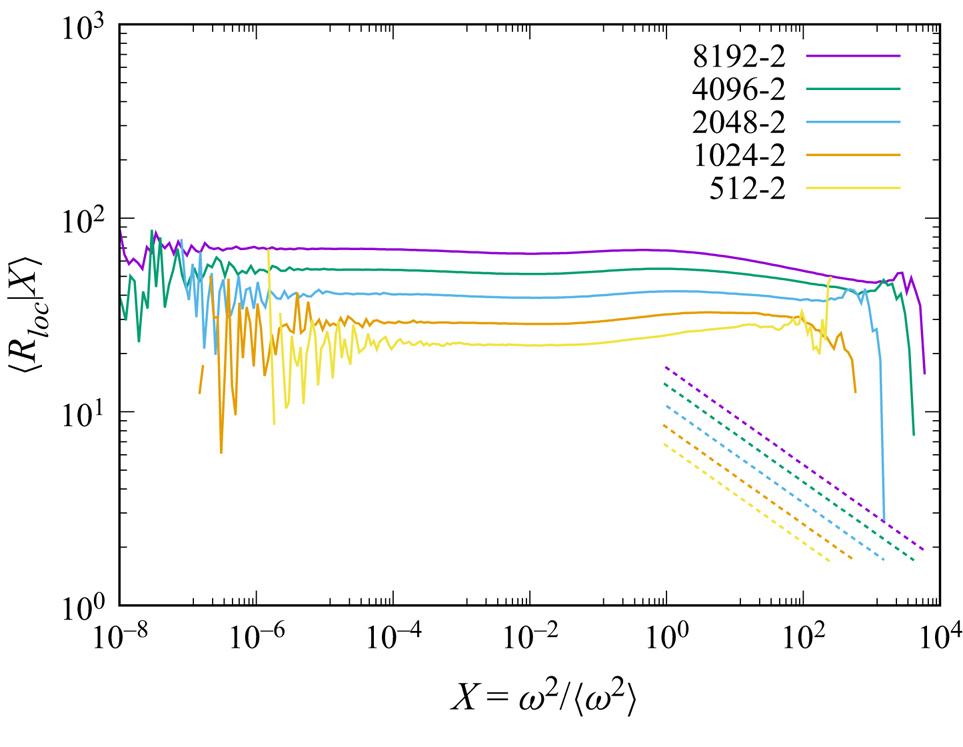
Figure 2. Plot of  $\langle R_{loc}| X \rangle$ vs
  $X= {{\omega ^{2}/\langle \omega ^{2} \rangle }}$ in runs 512-2, 1024-2,
  $\ldots$, 8192-2 (
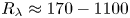 $R_\lambda \approx 170-1100$). Dashed lines show
  $\langle R_{loc}| X \rangle = (u' \eta /\nu )X^{-1/4}$ (see (4.16c)).
In order to see the potential influence of spatial resolution, we have compared  $\langle R_{loc} |X\rangle$ obtained by DNS at
  $R_\lambda \approx 268$ and
  $730$ with
  $k_{ max}\eta \approx 2$ with those obtained by DNS at similar
  $R_\lambda$ but with a lower resolution
  $k_{ max}\eta \approx 1$ and a higher resolution
  $k_{ max}\eta \approx 4$. The comparison is shown in figure 3. It is seen that although there are some differences between
  $\langle R_{loc} |X\rangle$ by DNS with
  $k_{ max}\eta \approx 1$ and
  $k_{ max}\eta \approx 2$ or 4, the difference between the plots for
  $k_{ max}\eta \approx 2$ and
  $4$ (solid and dashed lines) is not so significant, i.e. the plots agree well with each other, at least to the extent that can be seen in figure 3, except at low
  $X$ and large
  $X$, say, e.g.
  $X>10^{2}$. The comparison suggests that the result ‘that
  $\langle R_{loc}|X \rangle$ is almost independent of
  $X$ except at low and large
  $X$ at each
  $Re$’ noted above is not much affected by the resolution, provided that
  $k_{ max}\eta \approx 2$ or larger. In this paper we use the data by DNS with
  $k_{ max}\eta \approx 2$, unless otherwise stated.
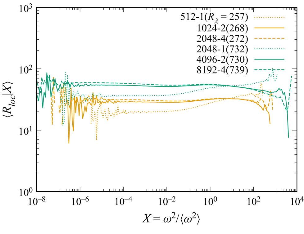
Figure 3. Comparison of  $\langle R_{loc}| X \rangle$ by DNS with the resolution
  $k_{ max}\eta \approx 2$ (runs 1024-2 and 4096-2) and those by a lower resolution
  $k_{ max}\eta \approx 1$ (runs 512-1, 2024-1) and a higher resolution
  $k_{ max}\eta \approx 4$ (runs 2048-4 and 8192-4).
After reading a preliminary version of this paper, an anonymous reviewer commented that the present study is related to the joint p.d.f. of the local energy transfer vs enstrophy studied in Faller et al. (Reference Faller2021). They found that the local energy transfer, defined as an inner product of vectors related to the velocity and the inertia forces, is proportional to  $\omega ^{2}$. The reviewer noted that we can expect the constancy of the ratio of local energy transfer to local viscous dissipation, if we approximate the local energy dissipation by
  $\nu \omega ^{2}$ (the equality holds exactly only for global averages). It is to be noted here that the local energy transfer studied in Faller et al. (Reference Faller2021) is defined in terms of the velocity difference between two points, so that it is invariant under any Galilean transformation. This suggests that the transfer is free from the so-called random sweeping effects by large eddies, while the term
  $({{\boldsymbol {u}}}\boldsymbol {\cdot }\boldsymbol {\nabla }){{\boldsymbol {u}}}$ used in the definition of
  $R_{loc}$, (1.1), in the present study is not invariant under Galilean transformation, and is in general dominated by the sweeping effect by large eddies. In the authors’ view, it is therefore questionable that the statistics of the ratio studied in Faller et al. (Reference Faller2021) are similar to those of
  $R_{loc}$.
Figure 1(c) (black dashed line) and figure 2 show that the dependence of  $\langle R_{loc}| X \rangle$ on the activeness
 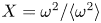 $X=\omega ^{2}/\langle \omega ^{2} \rangle$ is weak, i.e.
  $\langle R_{loc}| X \rangle$ is almost independent of
  $X$. The weakness of the dependence of the statistics of
  $R_{loc}$ on
  $X$ is also observed in figures 4 and 5. Figure 4 shows the plot of the pre-multiplied joint p.d.f.
  $F(Y) \equiv XYP(X,Y)$ at
  $X\equiv \omega ^{2}/\langle \omega ^{2} \rangle = 10^{n} \ (n=-5, -4, \ldots , 3)$ as a function of
  $Y=R_{loc}$. It is observed that the profiles of the curves are similar. The similarity is more pronounced in figure 5, which shows the plots of the normalised p.d.f.
  $f$ defined by
 \begin{equation} f(\xi) \equiv C F(Y)=C XY P(X,Y) \end{equation}
for any fixed  $X$, where
  $C$ is an appropriate normalization factor, which is chosen so that
 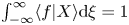 $\int _{-\infty }^{\infty } \langle f| X \rangle \textrm {d} \xi =1$, and
  $\xi =\xi (Y)$ is given by
 \begin{equation} \xi =\xi(Y)\equiv \log_{10} Y-\langle \log_{10} Y|X \rangle. \end{equation}
It is observed in figure 5 that the curves for different values of  $X$ overlap well, and
  $f(\xi )$ fits well to
  $f(\xi ) \propto \xi ^{8/3}$ and
  $\xi ^{-3}$ at
  $\xi \approx -2$ and
  $2$, respectively.
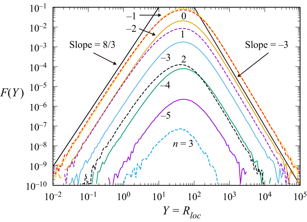
Figure 4. Pre-multiplied joint p.d.f.  $F(Y)\equiv XYP(X,Y)$ as a function of
  $Y=R_{loc}$ at
  $X=\omega ^{2}/\langle \omega ^{2}\rangle = 10^{n} \ (n=-5, -4, \ldots , 3)$ in run 8192-2. Solid lines are for
  $n=-5, -4, -3, -2, -1$ from bottom to top, and dashed lines are for
  $n=0, 1, 2, 3$ from top to bottom. Left and right solid lines show the slopes of
  $F \propto Y^{ 8/3}$ and
  $F \propto Y^{-3}$, respectively.
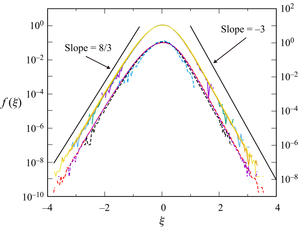
Figure 5. The same as figure 4 but for normalised p.d.f.  $f(\xi )$ defined by (3.4). To avoid excessive overlap, the lines for
  $n=0, 1,2,3$ are shifted downward and plotted with the right-hand side scale. Left and right solid lines show the slopes of
  $f \propto \xi ^{ 8/3}$ and
  $f \propto \xi ^{-3}$, respectively.
4. Local Reynolds number vs Re, and Re-dependence of moments
Given (1.3a,b), one might expect (1.4), i.e.  $Re \sim \langle R_{loc}\rangle$, but this is not so. In fact,
 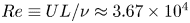 $Re\equiv UL/\nu \approx 3.67\times 10^{4}$ in the DNS field which yields figure 1, where
  $U=u'$ and
  $L$ is the characteristic length scale of energy-containing eddies defined by (2.1). The value
  $3.67\times 10^{4}$ is much larger than
  $\langle R_{loc} \rangle =67.2$. This implies that in the DNS,
 \begin{equation} Re \equiv \frac{UL}{\nu} \gg R_{loc} \equiv \frac{|({{\boldsymbol{u}}} \boldsymbol{\cdot} \boldsymbol{\nabla}) {{\boldsymbol{u}}}|}{|\nu \nabla^{2} {{\boldsymbol{u}}}|}. \end{equation}
 The large difference between  $\langle R_{loc} \rangle$ and
  $Re$ is not surprising because high
  $Re$ turbulence is a multi-scale phenomenon involving eddies of a very wide scale range. In general, the viscous term is not dominated by large eddies but by small ones. Hence, the second estimate of (1.4) is not necessarily correct. An estimate
  $\langle R_{loc} \rangle$ that is rough but better than (1.4) can be obtained by assuming that
(i) velocity gradients in the advective and viscous terms are dominated by small-scale eddies of size
$\sim \eta$ and characteristic velocity $\sim u_\eta$, and(ii) eddies of large scales (
$\sim L$) and small scales ($\sim \eta$) are statistically independent from each other (see, e.g. Tennekes Reference Tennekes1975).


These assumptions imply that
 \begin{equation} |({{{\boldsymbol{u}}}}\boldsymbol{\cdot} \boldsymbol{\nabla}) {{{\boldsymbol{u}}}}| \sim \frac{u' u_\eta}{\eta}, \quad |\nu \nabla^{2} {{{\boldsymbol{u}}}}|\sim \nu \frac{u_\eta}{\eta^{2}}, \end{equation}
instead of (1.3a,b). If we further introduce a bold assumption, i.e.
 \begin{equation} \left\langle \frac{ |({{\boldsymbol{u}}} \boldsymbol{\cdot} \boldsymbol{\nabla}) {{\boldsymbol{u}}}|}{ \nu |\nabla^{2} {{\boldsymbol{u}}}|}\right\rangle \sim \frac{\langle |({{\boldsymbol{u}}} \boldsymbol{\cdot} \boldsymbol{\nabla}) {{\boldsymbol{u}}}| \rangle }{ \langle \nu |\nabla^{2} {{\boldsymbol{u}}}|\rangle}, \end{equation}
then we obtain
 \begin{equation} \langle R_{loc} \rangle \sim \frac{u' \eta}{\nu} \ \propto Re^{1/4}, \end{equation}
at high  $Re$, where we assumed
  $u' \eta /\nu = u'/(\nu \left\langle\epsilon\right\rangle)^{1/4} \propto Re^{1/4}$ at high
  $Re$. The estimate (4.4) gives
 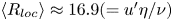 $\langle R_{loc} \rangle \approx 16.9(=u' \eta /\nu )$, which is much better than
  $3.67\times 10^{4}$ given by (1.4).
Equation (4.4) is also given by the estimate 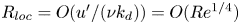 $R_{loc}= O(u'/(\nu k_d) )=O(Re^{1/4})$ by Orszag (Reference Orszag1977), who obtained it by using
 \begin{equation} \langle |({{{\boldsymbol{u}}}}\boldsymbol{\cdot} \boldsymbol{\nabla}){{{\boldsymbol{u}}}}|^{2} \rangle =O(u'^{2} \varOmega)= O( \langle\epsilon\rangle u'^{2}/\nu), \end{equation}
and
 \begin{equation} \langle |\nu \nabla^{2} {{{\boldsymbol{u}}}})|^{2} \rangle =O\left(\nu^{2} \int_0^{\infty} k^{4}E(k)\,\textrm{d}k \right) =O(\nu k_d^{2} \langle\epsilon\rangle ), \end{equation}
where  $\varOmega ^{2}=(1/2)\langle \omega ^{2} \rangle$ and
  $k_d\equiv 1/\eta$.
Figure 6 shows the plot of  $\langle R_{loc} \rangle$ vs
  $Re$ by DNS. The values
  $u'\eta /\nu$ and
  ${\langle |({{\boldsymbol {u}}} \boldsymbol {\cdot } \boldsymbol {\nabla }) {{\boldsymbol {u}}}| \rangle }/{ \langle |\nabla ^{2} {{\boldsymbol {u}}}|\rangle }$ in (4.3) are also plotted. This gives a direct check of (4.3); it is seen that the right-hand side of (4.3) is closer than
  $u'\eta /\nu$ to the left-hand side, i.e.
  $\langle R_{loc} \rangle$, although (4.3) is not exact as could be expected. It is also observed that the slope is not far from
  $1/4$, as predicted by (4.4), although it looks slightly steeper than
  $1/4$.
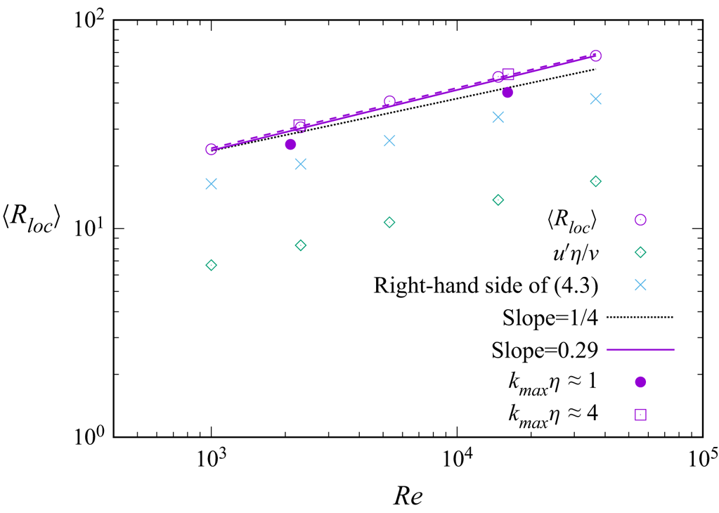
Figure 6. Plots of  $\langle R_{loc} \rangle$ (
 $\circ$),
  $u'\eta /\nu$ (
 $\diamond$) and
  $\langle |({{\boldsymbol {u}}} \boldsymbol {\cdot } \boldsymbol {\nabla }) {{\boldsymbol {u}}}| \rangle /\langle \nu |\nabla ^{2} {{\boldsymbol {u}}}|\rangle$ in (4.3) (
 $\times$) vs
  $Re$, in runs 512-2, 1024-2,
  $\ldots$, 8192-2. The symbols
  $\bullet$ and
  $\square$ show
  $\langle R_{loc} \rangle$ by runs 512-1, 2048-1 (
 $k_{ max}\eta \approx 1$) and runs 2048-4, 8192-4 (
 $k_{ max}\eta \approx 4$), respectively. Dashed, solid and dotted lines show the fit of (4.12), the slopes by the multi-fractal model and the slopes
  $1/4$, respectively.
The anonymous reviewer noted in § 3 commented that in the view of the reviewer the result that the slope of  $\langle R_{loc} \rangle$ is slightly steeper than
  $1/4$ can be easily explained by intermittency, and the use of the same arguments developed in Dubrulle (Reference Dubrulle2019) based on multi-fractal theory yields
  $\langle R_{loc} \rangle \sim Re^{0.29}$. (See Appendix A for the derivation of this result as well as (4.7)–(4.11a–d) and (4.16a–c) shown below.)
One can apply similar arguments not only to  $\langle R_{loc} \rangle$, but also to
  $\langle (R_{loc} )^{n} \rangle$ for
  $n\ne 1$. The application gives
 \begin{equation} \langle (R_{loc}) ^{n}\rangle \propto Re^{r_n}, \end{equation}
where
 \begin{equation} r_1=0.29, \quad r_2= 0.60, \quad r_3=0.93, \quad r_4=1.26. \end{equation}
If there was no intermittency,  $\langle (R_{loc} )^{n} \rangle \propto Re^{n/4}$, i.e.
  $r_n=n/4$, provided that
  $\eta /L \propto Re^{-3/4}$.
One can apply similar arguments also to the moments of the inertial and viscous forces. The application gives
 \begin{equation} \left\langle \left( \frac{ |({{{\boldsymbol{u}}}}\boldsymbol{\cdot} \boldsymbol{\nabla}) {{{\boldsymbol{u}}}}| }{ u'u_\eta/\eta } \right)^{n} \right\rangle \propto Re^{i_n}, \quad \left\langle \left( \frac{ |\nu \nabla^{2} {{{\boldsymbol{u}}}}| }{\nu u_\eta/\eta^{2}} \right)^{n} \right\rangle\propto Re^{v_n}, \end{equation}
where
 \begin{gather} i_1={-}0.04, \quad i_2=0, \quad i_3=0.13, \quad i_4=0.36, \end{gather}
 \begin{gather} v_1={-}0.03, \quad v_2= 0.13, \quad v_3=0.52, \quad v_4=1.26. \end{gather}
If there was no intermittency, the assumption (4.2a,b) would give  $i_n=v_n=0$ for any
  $n$.
$n$.
Figures 7, 8 and 9 show  $\langle (R_{loc})^{n} \rangle$,
  $\langle [ |({{{\boldsymbol {u}}}}\boldsymbol {\cdot } \boldsymbol {\nabla }) {{{\boldsymbol {u}}}}|/({u'u_\eta /\eta } )]^{n} \rangle$ and
 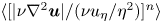 $\langle [ |\nu \nabla ^{2} {{{\boldsymbol {u}}}}|/(\nu u_\eta /\eta ^{2})]^{n}\rangle$, respectively, for
  $n=1,2,3$ and
  $4$ by DNS. A least square fitting of the DNS data in the figures to the form
 \begin{equation} \log_{10} \langle Y^{n} \rangle = a_n + b_n \log_{10} Re, \end{equation}
gives
 \begin{gather} r_1= 0.29, \quad r_2=0.58, \quad r_3=0.97, \quad r_4=1.85, \end{gather}
 \begin{gather} i_1={-}0.01, \quad i_2=0.03, \quad i_3=0.13, \quad i_4=0.31, \end{gather}
 \begin{gather} v_1={-}0.02, \quad v_2= 0.07, \quad v_3=0.25, \quad v_4=0.51, \end{gather}
where  $a_n$ and
  $b_n$ are constants, and
  $b_n=r_n, i_n$ and
  $v_n$ for
  $Y=R_{loc}$,
 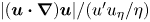 $|({{{\boldsymbol {u}}}}\boldsymbol {\cdot } \boldsymbol {\nabla }) {{{\boldsymbol {u}}}}| /(u'u_\eta /\eta )$ and
  $|\nu \nabla ^{2} {{{\boldsymbol {u}}}}|/(\nu u_\eta /\eta ^{2})$, respectively.
Figure 7. Plot of  $\langle (R_{loc} )^{n} \rangle$ vs
  $Re$ for
  $n=1,2,3$ and 4. Dotted lines show the slopes
  $n/4$. The meanings of the symbols and the solid and dashed lines are the same as in figure 6, but for
  $\langle (R_{loc} )^{n} \rangle$.
Figure 8. The same as in figure 7, but for  $\langle [ |({{{\boldsymbol {u}}}}\boldsymbol {\cdot } \boldsymbol {\nabla }) {{{\boldsymbol {u}}}}|/({u'u_\eta /\eta } )]^{n}\rangle$. The slopes for
  $i_n=0$ are omitted.
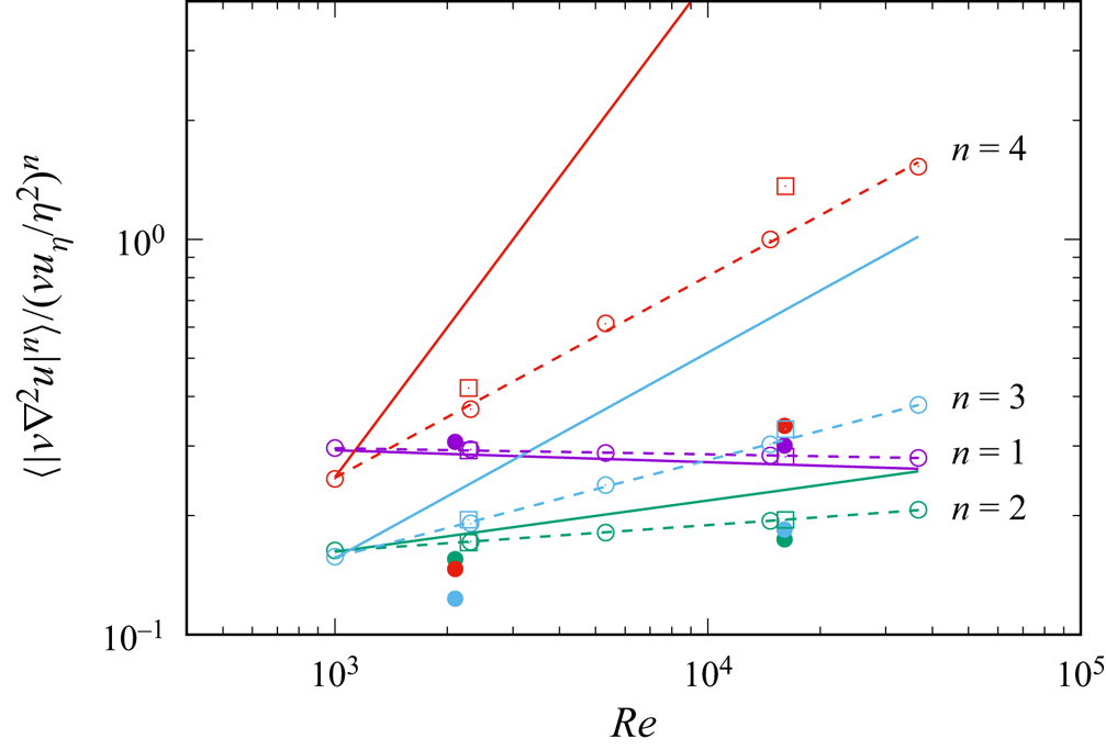
Figure 9. The same as in figure 7, but for  $\langle [ |\nu \nabla ^{2} {{{\boldsymbol {u}}}}|/(\nu u_\eta /\eta ^{2})]^{n}\rangle$. The slopes for
  $v_n=0$ are omitted.
Although a close inspection shows that the theoretical estimates (4.8a–d), (4.10a–d) and (4.11a–d) do not accurately agree with (4.13a–d), (4.14a–d) and (4.15a–d), especially for large  $n$, the theory captures well the tendency that the intermittency effect is considerably small for
  $n=1$ and
  $2$, and it is not so small for larger
  $n$, i.e.
  $n=3,4$. The numerical disagreement of the theory with the DNS especially for large
  $n$ is not surprising because the moments for large
  $n$ (in other words, moments including many ‘
 $\boldsymbol {\nabla }$’), are in general sensitive to the resolution. Figures 6–9, which include some data by DNS with a lower resolution (
 $k_{{max}} \eta \approx 1$) and higher resolution (
 $k_{{max}} \eta \approx 4$), give an idea on the potential influence of the resolution. The figures suggest that the influence of the resolution is not particularly significant for small
  $n$, say for
  $n=1,2$, provided that
  $k_{ max}\eta \approx 2$ or larger. By the way, the figures also suggest that, regarding the low-order moments for
  $n=1$ and
  $2$, the exponents by DNS with
  $k_{{max}} \eta \approx 1$ are not that different from those with
  $k_{{max}} \eta \approx 2$ or
  $4$.
$4$.
The disagreement between the theory and the DNS is not surprising also in view of the fact that the theory is based on assumptions which one may think to be questionable in a strict sense especially at finite  $Re$. Among them are the assumption of the statistical independence of eddies at small scales (
 $\sim \eta$) from those of eddies at large scales (
 $\sim L$) as noted in the derivation of (4.2a,b), and the assumption of applicability of the intermittency model not only to the active regions (large
  $X$-region) but also to the non-active regions (or ignoring the potential difference of statistics in non-active regions); it would not be surprising if the non-active regions may have non-negligible influence on low-order moments at finite
  $Re$.
$Re$.
By the way, as shown in Appendix A, the application of the idea of multi-fractal theory to the vorticity yields
 \begin{equation} \frac{|({{{\boldsymbol{u}}}}\boldsymbol{\cdot} \boldsymbol{\nabla}) {{{\boldsymbol{u}}}}|}{u'u_\eta/\eta} \sim X^{1/2}, \quad \quad \frac{|\nu \nabla^{2} {{{\boldsymbol{u}}}}|}{\nu u_\eta/\eta^{2}} \sim X^{3/4}, \quad \frac{R_{loc}}{u'\eta/\nu} \sim X^{{-}1/4}, \end{equation}
where  $X \equiv \omega ^{2}/\langle \omega ^{2} \rangle$. Concerning the inertial force, the exponent
  $1/2$ in (4.16a) is in good agreement with the exponent of the conditional average for a given
  $X$ by the DNS (see (3.2)). As regards the viscous force and
  $R_{loc}$, (4.16b,c) is consistent with the increase (decrease at high
  $R_\lambda$) of the conditional average of the viscous force (
 $R_{loc}$) with
  $X$ at large
  $X$ in the DNS as seen in figures 1(b,c) and 2, but the exponents
  $3/4$ and
  $-1/4$ seem not that close to those of the conditional averages by the DNS.
At present, it is not known if the agreement between the theory and DNS would be improved by increasing the resolution and/or  $Re$ of DNS.
5. Influence of energy dissipation rate $\epsilon$

Figures 10, 11 and 12 show the same plots as figures 1, 2 and 5, respectively, but for  $X=\epsilon /\langle \epsilon \rangle$, where
 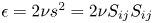 $\epsilon =2 \nu s^{2}=2 \nu S_{ij}S_{ij}$. Overall, figures 10, 11 and 12 are similar to figures 1, 2 and 5, respectively. In particular, it is observed that
(i) the pre-multiplied joint p.d.f.s
$XYP(X, Y)$ in figures 10(a) and 10(b) are similar to each other, like those in figures 1(a) and 1(b), where $Y=|({{\boldsymbol {u}}} \boldsymbol {\cdot } \boldsymbol {\nabla }) {{\boldsymbol {u}}}|/(u' u_\eta /\eta )$ and $Y=| \nu \nabla ^{2} {{\boldsymbol {u}}}|/(\nu u_\eta /\eta ^{2})$ in figures 10(a) and 10(b), respectively;(ii) the conditional averages
$\langle Y {{\big {\vert }}}X \rangle$ increase with $X$ at large $X$, and the increases are nearly proportional to $X^{1/2}$, in figure 10(a,b) just like in figure 1(a,b), where $X={{\omega ^{2}/\langle \omega ^{2} \rangle }}$ in figure 1, whereas $X={{\epsilon /\langle \epsilon \rangle }}$ in figure 10;(iii) both of the conditional averages of the inertial and viscous forces in the DNS field are smaller than those in the random field at small
$X$, and the depression of conditional averages occurs only for small $X$, but not for large $X$;(iv) the dependence of the conditional average
$\langle R_{loc}{{\big {\vert }}}X \rangle$ on $X$ is weak in figures 10(c) and 11, just as in figures 1(c) and 2;(v) the normalised p.d.f.
$f(\xi )$ given by (3.4) is almost independent of $X$ as seen in the overlap of the curves in figure 12, just as in figure 5.

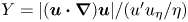


Figure 10. The same as figure 1 but with  $X=s^{2}/\langle s^{2}\rangle = \epsilon /\langle \epsilon \rangle$.
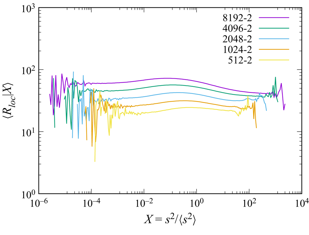
Figure 11. The same as figure 2 but with  $X=s^{2}/\langle s^{2}\rangle = \epsilon /\langle \epsilon \rangle$. Lines for
  $\langle R_{loc}| X \rangle = (u' \eta /\nu ) X^{-1/4}$ are omitted.
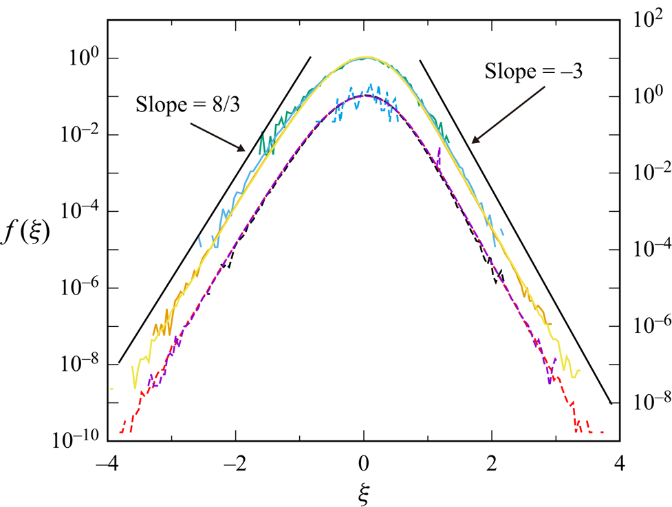
Figure 12. The same as figure 5 but with 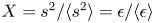 $X=s^{2}/\langle s^{2}\rangle = \epsilon /\langle \epsilon \rangle$. The line for
  $n=-5$ is omitted.
It is shown in the same way as the derivation of (4.16a–c) in Appendix A that one has (4.16a–c) not only for  $X={{\omega ^{2}/\langle \omega ^{2} \rangle }}$, but also for
  $X={{\epsilon /\langle \epsilon \rangle }}$. As in the case of
  $X=\omega ^{2}/\langle \omega ^{2} \rangle$, the exponent
  $1/2$ in (4.16a) by the intermittency model is in good agreement with DNS (figure 10(a)), but the exponents
  $3/4$ and
  $-1/4$ in (4.16b,c) look to be not close to those of the conditional averages by DNS, in figures 10(b,c) and 11.
6. Conclusion
In this paper we studied the statistics of the local Reynolds number  $R_{loc}$, defined as the ratio of inertial to viscous forces, in DNS of forced turbulence in a periodic box with the Taylor microscale Reynolds number
  $R_\lambda$ up to approximately
  $1100$. Particular attention is paid to the influence of the local activeness of the field on the statistics of
  $R_{loc}$. We analysed the joint p.d.f.
  $P(X,Y)$, where
  $X=X({{\boldsymbol {x}}},t)$ is a measure representing the activeness at
  $({{\boldsymbol {x}}},t)$, and
  $Y=Y({{\boldsymbol {x}}},t)$ is the magnitude of the inertial or viscous force under appropriate normalization, or the ratio
  $R_{loc}({{\boldsymbol {x}}},t)$. Among the measures that can represent activeness, we used the normalised squared vorticity
  ${{\omega ^{2}/\langle \omega ^{2} \rangle }}$ and the normalised energy dissipation rate
  ${{\epsilon /\langle \epsilon \rangle }}$.
The analysis of the DNS data shows that both of the conditional averages of inertial and viscous forces for a given activeness  $X$ represented by
  $X={{\omega ^{2}/\langle \omega ^{2} \rangle }}$ or
  $X={{\epsilon /\langle \epsilon \rangle }}$ increase nearly in proportion to
  $X^{1/2}$ in active regions. By contrast, the conditional average of
  $R_{loc}$ for a given
  $X$ is almost independent of
  $X$ over a wide range of
  $X$, i.e. the increase in the conditional averages of inertia and viscous forces at large
  $X$ cancel each other. A comparison of the DNS field with a structureless random field having the same energy spectrum suggests that there is a certain mechanism in the NS dynamics which suppresses the increase of the
  $R_{loc}$ with the activeness, at large
  $X$.
$X$.
Not only the conditional average  $R_{loc}$, but also the conditional p.d.f. of
  $R_{loc}$ for a given
  $X$ is observed to be almost independent of
  $X$ after an appropriate normalization. Under an appropriate normalization, the p.d.f. is almost independent of
  $X$ and fits well to certain simple power law forms in certain ranges of
  $X$ for both
  $X=\omega ^{2}/\langle \omega ^{2} \rangle$ and
  $X={{\epsilon /\langle \epsilon \rangle }}$.
The DNS data also show that the average  $\langle R_{loc}\rangle$ over the entire space is much smaller than the global Reynolds number defined by
  $Re\equiv UL/\nu$, and scales with
  $Re$ as
  $\propto Re^{\alpha }$, where
  $L$ and
  $U$ are respectively the integral length scale and root mean square of the fluctuating velocity in one direction, and
  $\alpha$ is approximately 1/4, which is consistent with the estimate
  $R_{loc}=O(Re^{1/4})$ by Orszag (Reference Orszag1977), but a little larger than 1/4. This result is shown to be consistent with the simple multi-fractal model of intermittency of Dubrulle (Reference Dubrulle2019). The idea of the model is applicable also to the estimates of the
  $n$th order moments of
  $R_{loc}$ as well as those of inertial and viscous forces. Although the theoretical estimates do not accurately agree with DNS, the theory captures well the tendency for the influence of intermittency on the Re scaling of the moments to generally increase with n.
Acknowledgements
The authors are grateful to anonymous reviewers for valuable comments, in particular those on the intermittency model discussed in § 4. Y.K. is grateful to P.A. Davidson, K. Moffatt, K.R. Sreenivasan and D. Tranah for their warm encouragements at an early stage of this study. Some results of the analysis of  $R_{loc}$ and the influence of squared vorticity using DNS data at
  $R_\lambda\approx 429$ were reported at a meeting held at the Kavli Institute for Theoretical Physics, UC Santa Barbara, (web site: http://online.kitp.ucsb.edu/online/turbulence11/kaneda/).
Funding
This study was partly supported by JSPS KAKENHI, grant numbers JP16H06339, JP19H00641 and 20H01948. The computational resources of the K computer and the supercomputer Fugaku provided by the RIKEN Advanced Institute for Computational Science through the HPCI System Research project (Projects ID: hp180109, ID: hp190076, ID: hp200184 and ID: hp210138) were partly used in this study. This study was also partly supported by ‘Joint Usage/Research Center for Interdisciplinary Large-scale Information Infrastructures’ (Projects ID: jh190068, ID: jh200021 and ID: jh210034).
Declaration of interests
The authors report no conflict of interest.
Data availability statement
The data that support the findings of this study are available in the electronic supplementary material upon reasonable request.
Appendix A. Derivation of (4.7)–(4.11a–d) and (4.16a–c)
We assume here that there exists a local ‘Kolmogorov scale’  $\eta _h$ for each local exponent
  $h$. (Such an
  $\eta _h$ scales with viscosity like
  $\propto \nu ^{1/(1+h)}$, and if
  $h=1/3$ we recover the Kolmogorov microscale.) Then, by replacing
  $u_\eta$ and
  $\eta$ in (4.2a,b) to
  $u'(\eta _h/L)^{h}$ and
  $\eta _h$, respectively, we have
 \begin{equation} |({{{\boldsymbol{u}}}}\boldsymbol{\cdot} \boldsymbol{\nabla}) {{{\boldsymbol{u}}}}| \sim u'\left[ u'\left( \frac{\eta_h}{L} \right)^{h}\right] \frac{1}{\eta_h}, \quad \quad |\nu \nabla^{2} {{{\boldsymbol{u}}}} |\sim \nu \left[ u' \left( \frac{\eta_h}{L} \right)^{h} \right]\frac{1}{ (\eta_h) ^{2}}, \end{equation}
instead of (4.2a,b), so that
 \begin{equation} R_{loc} \sim \frac{u'}{\nu}\eta_h \sim Re\frac{\eta_h}{L}, \end{equation}
which gives
 \begin{equation} \langle R_{loc} \rangle \sim Re \left\langle \frac{\eta_h}{L} \right\rangle. \end{equation}
If there was no intermittency,  $\eta _h=\eta$ everywhere and we recover the
  $Re^{1/4}$ scaling (4.4). But if there is intermittency, described by a multi-fractal spectrum
  $C(h)$, we obtain instead
 \begin{equation} \langle R_{loc} \rangle \propto Re^{1-\chi(1)}, \end{equation}
where
 \begin{equation} \chi(1)= \min_h \chi(1;h), \quad \chi( \xi;h)\equiv \left( \frac{\xi+C(h)}{1+h} \right), \end{equation}
in which we have used 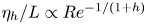 $\eta _h/L \propto Re^{-1/(1+h)}$. Using a parabolic fit for
  $C(h)$, i.e.
 \begin{equation} C(h)=\frac{1}{2b}(h-a)^{2}, \quad b=0.045, \quad a=\frac{1}{3}+\frac{3b}{2} \end{equation}
(see Dubrulle Reference Dubrulle2019), we obtain 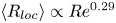 $\langle R_{loc} \rangle \propto Re^{0.29}$. The authors are grateful to an anonymous reviewer for these comments. Readers may refer to, for example, Frisch (Reference Frisch1995), Dubrulle (Reference Dubrulle2019) and the references cited therein for more about multi-fractal models.
Similar arguments can be applied also to  $\langle (R_{loc} )^{n} \rangle$ for
  $n\ne 1$. Equation (A2) and the multi-fractal model with (A6) give (4.7), where
 \begin{equation} r_n=n-\min_h \chi(n;h). \end{equation}
This gives among others (4.8a–d).
Similar arguments can be applied also to the moments of the inertial and viscous forces. Since (A1) can be written as
 \begin{equation} \frac{|({{{\boldsymbol{u}}}}\boldsymbol{\cdot} \boldsymbol{\nabla}) {{{\boldsymbol{u}}}}|}{u'u_\eta/\eta} \sim Re^{{-}1/2}\left( \frac{\eta_h}{L} \right)^{h-1}, \quad \frac{|\nu \nabla^{2} {{{\boldsymbol{u}}}}|}{\nu u_\eta/\eta^{2}} \sim Re^{{-}5/4 }\left( \frac{\eta_h}{L} \right)^{h-2}, \end{equation}
(A1) and the multi-fractal model with (A6) give (4.9a,b), where
 \begin{equation} i_n ={-}\frac{n}{2}-\min_h \chi(n(h-1);h) , \quad v_n ={-}\frac{5n}{4}-\min_h \chi(n(h-2);h), \end{equation}
and we have used 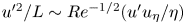 $u'^{2}/L \sim Re^{-1/2}({u'u_\eta /\eta } )$ and
 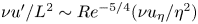 $\nu u'/L^{2} \sim Re^{-5/4 }(\nu u_\eta /\eta ^{2})$. Consequently, we have among others (4.10a–d) and (4.11a–d). The result
  $i_2=0$ in (4.10b) implies that
  $\min _h \chi (2(h-1);h)=-1$. This is consistent with the relation
  $\langle \epsilon \rangle \equiv 2 \nu \langle S_{ij}S_{ij}\rangle \propto Re^{0}$ obtained by Frisch & Vergassola (Reference Frisch and Vergassola1991) in the framework of multi-fractal theory.
The argument leading to (A1) can be applied also to the vorticity field. By setting  $\omega \sim u/\eta _h$ with
  $u\sim u'(\eta _h/L)^{h}$, we have
  $\omega \sim u'(\eta _h/L)^{h}/\eta _h =(u'/L)(\eta _h/L)^{h-1}$. This implies that
 \begin{equation} X^{1/2} =\frac{\omega}{u_\eta/\eta} \sim Re^{{-}1/2}\left( \frac{\eta_h}{L} \right)^{h-1}, \end{equation}
where we have used  $u'/L \sim Re^{-1/2}(u_\eta /\eta )$ and
  $X = \omega ^{2}/\langle \omega ^{2} \rangle = \omega ^{2}/(u_\eta /\eta )^{2}$, the last equality of which is verified by
 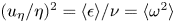 $(u_\eta /\eta )^{2}=\langle \epsilon \rangle /\nu =\langle \omega ^{2}\rangle$. It is shown by straightforward algebra that (A8) and (A10) with
  $(\eta _h/L) \sim Re^{-1/(1+h)}$ give (4.16a–c).


