3.1 Time-averaged statistics

The distributions of the mean velocity in wall coordinates, $\langle \overline{U_{x}}^{+}\rangle$ , for turbulent channel flows of Newtonian and viscoelastic solutions are displayed in figure 1(a). The bar indicates the time average and ‘ $\langle \,\rangle$ ’ denotes the $x$ – $y$ plane average. The grey circles represent the Newtonian mean velocity profile at $Re_{\unicode[STIX]{x1D70F}_{0}}=180$ while the other symbols represent the viscoelastic flows. In the viscous sublayer ( $0<z^{+}<5$ ), where the total stress is predominantly associated with viscous effects, the mean velocities converge to the same linear shape $\langle \overline{U_{x}}^{+}\rangle =z^{+}$ represented by the solid grey line. As the wall distance increases, the Reynolds stress becomes important and comparable to the viscous stress within the Newtonian buffer layer ( $5<z^{+}<30$ ). Then, the Newtonian mean velocity departs quickly from the linear profile, taking on a logarithmic dependence on $z^{+}$ (grey dashed line) in the Newtonian log-law region, $z^{+}>30$ , $\langle \overline{U_{x}}^{+}\rangle =(1/\unicode[STIX]{x1D705})\ln (z^{+})+A_{1}$ where $\unicode[STIX]{x1D705}$ is commonly called the von Kármán coefficient ( $1/\unicode[STIX]{x1D705}$ is the slope) and $A_{1}$ is the intercept at $z^{+}=1$ . For Newtonian channel flows over a hydraulically smooth wall, $\unicode[STIX]{x1D705}=0.4$ and $A_{1}=5.5$ (Kim, Moin & Moser Reference Kim, Moin and Moser1987). In order to better describe our results, we use the boundaries of the viscous sublayer, the buffer layer and the log-law Newtonian regions to define regions I, II and III, respectively. It is important to emphasize, however, that regions II and III do not necessarily represent the buffer layer and the log-law region for the viscoelastic cases, since the polymers can increase the former layer, reducing the latter.

Figure 1. Mean velocity profiles in the streamwise direction (a), $\langle \overline{U_{x}}^{+}\rangle$ , and normal components of the Reynolds stress (b–d) for Newtonian and viscoelastic channel flows, against the normalized wall distance.

The interactions between the viscoelastic fluid dynamics and the turbulent flow dynamics result in changes in the mean velocity profile relative to the Newtonian fluid. The polymer drag reduction phenomenon leads to an increased bulk mean velocity, as observed by comparing the viscoelastic profiles plotted in figure 1. When a high enough polymer concentration is used, the maximum level of drag reduction (MDR) is attained. In that state, the velocity profile is commonly represented by the Virk’s asymptote (Virk et al. Reference Virk, Mickley and Smith1970), $\langle \overline{U_{x}}^{+}\rangle =11.7\ln (z^{+})+17.8$ which is a matter of recent controversy (White, Dubief, & Klewicki Reference White, Dubief and Klewicki2012). Experimental and recent numerical results based on DNS (Escudier, Presti & Smith Reference Escudier, Presti and Smith1999; Ptasinski et al. Reference Ptasinski, Nieuwstadt, Van den Brule and Hulsen2001; Escudier, Nickson, & Poole Reference Escudier, Nickson and Poole2009; Thais et al. Reference Thais, Gatski and Mompean2012) indicate a parallel upward shift of the logarithmic region of the mean velocity profile with increasing DR, which is clearly perceived at high Reynolds numbers (see Thais et al. Reference Thais, Gatski and Mompean2013). Such a behaviour suggests a significant extension of the buffer layer region into the channel caused by the polymers. For viscoelastic fluids, the cross-over to a presumed Newtonian plug flow occurs at a distance from the wall where the Reynolds stress momentum flux is no longer negligible compared to that of the polymer/viscous stress. Figure 1(b–d) show the normal components of the Reynolds stress tensor, whose components are defined as the time average of the velocity fluctuation product ( $\overline{{u^{\prime }}_{i}{u^{\prime }}_{j}}^{+}$ ). The mean effect of the polymer on the turbulence is anisotropic and induces an increase in the streamwise normal Reynolds stress component (figure 1 b), while weakening both the spanwise (figure 1 c) and the wall-normal (figure 1 d) terms, as experimentally found by many researchers such as Pinho & Whitelaw (Reference Pinho and Whitelaw1990), Warholic, Massah & Hanratty (Reference Warholic, Massah and Hanratty1999) and White, Somandepalli & Mungal (Reference White, Somandepalli and Mungal2004). This effect is more pronounced as the elasticity increases, as indicated by the solid black arrows. In the most elastic flow at $Re_{\unicode[STIX]{x1D70F}_{0}}=180$ (orange inverted triangles), for instance, the peak of  $\langle \overline{{u^{\prime }}_{x}{u^{\prime }}_{x}}^{+}\rangle$ moves from $z^{+}\approx 12$ (region II) to $z^{+}\approx 32$ and its value is one order of magnitude greater than the Newtonian one (grey open circles). In addition, the other components also shift away from the wall, but their peaks decrease by one order of magnitude compared to the Newtonian flow. Since vortices produce significant transverse fluctuations, the reduction of both ${u^{\prime }}_{y}$ and ${u^{\prime }}_{z}$ suggests a strong interaction between these intermittent structures and polymers (Dubief et al. Reference Dubief, White, Terrapon, Shaqfeh, Moin and Lele2004). Lastly, the dashed arrows indicate that the normal Reynolds stress components are an increasing function of $Re_{\unicode[STIX]{x1D70F}_{0}}$ . Their peaks move towards the channel centre with increasing Reynolds number.

Figure 2. (a) Evolution of the mean relative polymer extension, $\langle \text{tr}(\overline{\unicode[STIX]{x1D63E}})/L^{2}\rangle$ , against the normalized wall distance. (b) Effects of mean shear stress profile on polymer extension.

The variations in polymer mean stresses across the channel can be highlighted by analysing the polymer mean stretch, which is linked with the former by the Peterlin function (2.3). The distribution of the relative polymer mean stretch $\langle \text{tr}(\overline{\unicode[STIX]{x1D63E}})/L^{2}\rangle$ as a function of $z^{+}$ is displayed in figure 2(a), for all viscoelastic cases studied in the present paper. As a common point, the polymer molecules exhibit a significant extension at the wall, which increases in the buffer layer, where its peak is attained. This peak magnitude, as well as its location, is a decreasing function of $L$ , but increases with increasing $Wi_{\unicode[STIX]{x1D70F}_{0}}$ (these trends are discussed in § 4.1). As the wall distance increases further, $\langle \text{tr}(\overline{\unicode[STIX]{x1D63E}})/L^{2}\rangle$ becomes less pronounced until achieving its minimum level at $z^{+}=180$ . A very simple method to clarify the polymer stretching mechanism consists in solving (2.4) using different mean velocity profiles. The result is illustrated in figure 2(b), where the less elastic flow is considered (grey open circles), as well as the polymer extension produced in this fluid by a turbulent-channel-like velocity profile $\overline{U_{x}}=(9/8)[1-(z/h)^{8}]$ (Dallas et al. Reference Dallas, Vassilicos and Hewitt2010). As the derivative of the mean velocity with respect to the wall-normal direction increases, the polymers stretch considerably, due to the increase of the shear stress. More specifically, the profile of $\langle \text{tr}(\overline{\unicode[STIX]{x1D63E}})/L^{2}\rangle$ follows the mean viscous shear stress feature. Comparing the relative polymer extensions obtained from a turbulent-like mean velocity profile (orange inverted triangles) and DNS results (grey open circles), it is interesting to observe that both curves depart from the same level ( ${\approx}0.54$ ), at $z^{+}=0$ . However, as the wall distance increases, the discrepancy between them becomes pronounced. In fact, near the wall, the increasing $\langle \text{tr}(\overline{\unicode[STIX]{x1D63E}})/L^{2}\rangle$ noticed for the grey circles curve suggests that in this region there is a particular flow topology capable of producing an increase in the polymer extension beyond the viscous mean shear level represented by the orange inverted triangles. In other words, the viscous mean stress is responsible for a relevant polymer stretching, which is incremented since the turbulent structures interact with the polymer molecules, providing a supplementary polymer extension. We believe these intermittent polymer–turbulence interactions are also responsible for the polymer coil–stretch process, which will be analysed in later subsections from statistical and tensorial perspectives.

All the trends discussed above considering $Re_{\unicode[STIX]{x1D70F}_{0}}=180$ are also observed at higher zero shear friction Reynolds numbers, as previously reported by Thais et al. (Reference Thais, Gatski and Mompean2012) and Thais et al. (Reference Thais, Gatski and Mompean2013).

4.1 Polymer stretching

The three-dimensional structures shown in figure 3 represent the isosurfaces of the vortical regions, defined as the positive second invariant of the velocity gradient tensor, $\unicode[STIX]{x1D735}\boldsymbol{u}$ , in Newtonian (a) and viscoelastic (b–e) flows. For incompressible flows, the second invariant of $\unicode[STIX]{x1D735}\boldsymbol{u}$ , $Q$ , can be used to identify vortical structures, the so-called $Q$ -criterion (see Hunt et al. Reference Hunt, Wray and Moin1988), and simplified as

which indicates the spatial regions where the Euclidean norm of the rate-of-rotation tensor, $\Vert \unicode[STIX]{x1D652}\Vert$ , dominates that of the rate of strain, $\Vert \unicode[STIX]{x1D63F}\Vert$ (the Euclidean norm of a generic second-order tensor $\unicode[STIX]{x1D63C}$ is $\Vert \unicode[STIX]{x1D63C}\Vert =\sqrt{\text{tr}(\unicode[STIX]{x1D63C}\boldsymbol{\cdot }\unicode[STIX]{x1D63C}^{\unicode[STIX]{x1D64F}})}$ ). These structures follow an organized hierarchy across the channel. In the vicinity of the wall ( $z^{+}<20$ ), eddies are found to be pairs of counter-rotating quasi-streamwise vortices, while for $z^{+}>30$ , these eddies resemble hairpins (the so-called horseshoe vortices). The formation of such morphologies is induced by combined second-quadrant ejection ( $u_{x}^{\prime }<0,u_{z}^{\prime }>0$ ; Q2 event) and fourth-quadrant sweep ( $u_{x}^{\prime }>0,u_{z}^{\prime }<0$ ; Q4 event) events within the flow (see Adrian Reference Adrian2007). Specifically, the hairpin vortices are composed of three well defined parts. The legs are regions of rotation quasi-aligned with the streamwise direction. The head is a rotation part aligned with the spanwise direction. The necks are the connections between the legs and the head of the hairpin. These three parts, as well as the velocity fluctuations associated with them, can be seen in detail in figure 4, where a typical hairpin extracted from our less elastic flow ( $Re_{\unicode[STIX]{x1D70F}_{0}}=180$ , $Wi_{\unicode[STIX]{x1D70F}_{0}}=50$ and $L=30$ ) is coloured by the $Q$ events.

Figure 4. Typical hairpin extracted from a viscoelastic flow ( $Re_{\unicode[STIX]{x1D70F}_{0}}=180$ ; $Wi_{\unicode[STIX]{x1D70F}_{0}}=50$ ; $L=30$ ) with $Q=0.7$ and coloured by the Q1 ( $u_{x}^{\prime }>0,u_{z}^{\prime }>0$ ), Q2 ( $u_{x}^{\prime }<0,u_{z}^{\prime }>0$ ), Q3 ( $u_{x}^{\prime }<0,u_{z}^{\prime }<0$ ) and Q4 ( $u_{x}^{\prime }>0,u_{z}^{\prime }<0$ ) events.

Comparing figure 3(a–e), it can be seen that the number of vortices with a value of the $Q$ -criterion equal to 0.7 decreases with increasing elasticity ( $We$ and $L$ ). For $Wi_{\unicode[STIX]{x1D70F}_{0}}=115$ and $L=100$ , which provides $DR=62.3\,\%$ , the vortices with $Q=0.7$ are completely gone and the vortices with $Q=0.1$ (figure 3 e) are only found close to the walls. In viscoelastic flows, the vortical structures are significantly weaker than in the Newtonian flow, which is considered fundamental evidence of the polymer–turbulence interactions and the consequent drag reduction (Terrapon et al. Reference Terrapon, Dubief, Moin, Shaqfeh and Lele2004; Kim et al. Reference Kim, Li, Sureshkumar, Balachandar and Adrian2007, Reference Kim, Adrian, Balachandar and Sureshkumar2008; White & Mungal Reference White and Mungal2008). As the elasticity increases, some characteristics of the vortices change: their thicknesses and streamwise lengths increase, while their strengths weaken, which is clearly observed by comparing figure 3(a,e). Furthermore, the vortices become more parallel to the wall. In the log-law region, the hairpin head is strongly weakened. It has been experimentally and numerically shown that in drag reducing flows, the streamwise component of the Reynolds normal stresses increases relative to the Newtonian case, while the other components of the Reynolds stress tensors decrease (Wei & Willmarth Reference Wei and Willmarth1992; Warholic et al. Reference Warholic, Massah and Hanratty1999; Ptasinski et al. Reference Ptasinski, Nieuwstadt, Van den Brule and Hulsen2001; Kim et al. Reference Kim, Li, Sureshkumar, Balachandar and Adrian2007; Thais et al. Reference Thais, Gatski and Mompean2012). These variations seem to be closely connected with the coil–stretch polymer transition and the consequent vortex structural changes (Dimitropoulos et al. Reference Dimitropoulos, Dubief, Shaqfeh, Moin and Lele2005). The colours in figure 3(b–e) indicate the relative polymer stretch, $\text{tr}(\unicode[STIX]{x1D63E})/L^{2}$ . The $y$ – $z$ planes show that for all four viscoelastic flows, the polymers are more stretched close to the wall (yellow and red regions). In contrast, the polymer extensions are less pronounced in the middle of the channel (blue regions). The isosurface colours and those of the intersections between vortical structures and $y$ – $z$ planes show that the polymers are more extended around the near-wall vortices.

Figure 5. Normalized conformation tensor as a function of the normalized wall distance. Streamwise normal components of $\unicode[STIX]{x1D63E}$ and $\text{tr}(\unicode[STIX]{x1D63E})/L^{2}$ (open and solid in a, respectively). Spanwise normal component of $\unicode[STIX]{x1D63E}$ (b). Wall-normal component of $\unicode[STIX]{x1D63E}$ (c). Cross-components (d).

The stretching of the polymers can be seen more clearly in figure 5(a), where the evolution of the $x$ – $y$ -plane-averaged normalized trace of the instantaneous conformation tensor, $\langle \text{tr}(\unicode[STIX]{x1D63E})/L^{2}\rangle$ , is plotted against the wall distance $z^{+}$ (solid symbols) together with the normalized streamwise normal component of the conformation tensor, $\langle C_{xx}/L^{2}\rangle$ (open symbols). The percentage of polymer extension, $\langle \text{tr}(\unicode[STIX]{x1D63E})/L^{2}\rangle$ , is relatively high at the wall, achieving a peak in the very near-wall region ( $z^{+}<20$ ), the exact location of which varies with $L$ and $Wi_{\unicode[STIX]{x1D70F}_{0}}$ . This peak is commonly associated with the streamwise vortices (see Dubief et al. Reference Dubief, White, Terrapon, Shaqfeh, Moin and Lele2004; Dimitropoulos et al. Reference Dimitropoulos, Dubief, Shaqfeh, Moin and Lele2005; Dallas et al. Reference Dallas, Vassilicos and Hewitt2010). After this point, $\langle \text{tr}(\unicode[STIX]{x1D63E})/L^{2}\rangle$ starts to decrease, until reaching its minimum at the channel centre. In comparing the grey solid circles with the red solid diamonds, or the blue solid triangles with the green solid squares, it can be clearly seen that $\langle \text{tr}(\unicode[STIX]{x1D63E})/L^{2}\rangle$ decreases with increasing $L$ , for fixed $Re_{\unicode[STIX]{x1D70F}_{0}}$ and $Wi_{\unicode[STIX]{x1D70F}_{0}}$ , which suggests that the large polymer molecules could be less susceptible to chain scission degradation (Pereira & Soares Reference Pereira and Soares2012). A further comparison of the grey solid circles with the blue solid triangles, or of the red solid diamonds with the green solid squares, reveals that the relative polymer extension becomes greater as the friction Weissenberg number increases, since higher values of the polymer time scale induce the polymer molecules to be influenced by a wider spectrum of time scales of the flow (Dallas et al. Reference Dallas, Vassilicos and Hewitt2010). Figure 5(a) also shows that the dominant contribution to the trace of the conformation tensor comes from $C_{xx}$ , i.e. $\langle \text{tr}(\unicode[STIX]{x1D63E})/L^{2}\rangle \approx \langle C_{xx}/L^{2}\rangle$ (especially near the wall and for the highest value of $L$ , $L=100$ ). This distribution suggests a significant stretching of the polymers in the streamwise direction. The other component with a non-zero wall value is the off-diagonal component $C_{xz}$ , normalized and displayed in figure 5(d). However, its value at the wall is almost two orders of magnitude smaller than that of the $C_{xx}$ component. Moreover, as $Wi_{\unicode[STIX]{x1D70F}_{0}}$ and $L$ increase, the profile of $\langle C_{xz}/L^{2}\rangle$ follows the same tendencies noted in figure 5(a), reaching its peaks at $z^{+}$ not much different from those observed for $C_{xx}$ . The peak magnitude of the off-diagonal component $C_{xz}$ is comparable to that of the $C_{zz}$ component (plotted in figure 5 b), although both are only slightly smaller than the peak magnitude of the $C_{yy}$ component (shown in figure 5 c). It is worth noting that $\langle C_{xz}/L^{2}\rangle$ is an increasing function of the molecular relaxation time (the variations of which are here computed by changing $Wi_{\unicode[STIX]{x1D70F}_{0}}$ at fixed $Re_{\unicode[STIX]{x1D70F}_{0}}$ ) although a saturation effect is observed when increasing the elasticity (the red diamonds and green square curves are close). This saturation effect is also seen for $C_{zz}$ (figure 5 b) and $C_{yy}$ (figure 5 c). The peak magnitude of the normal components $C_{zz}$ and $C_{yy}$ are both one order of magnitude smaller than that of the $C_{xx}$ component, starting with a zero wall value. Lastly, as $Wi_{\unicode[STIX]{x1D70F}_{0}}$ increases, $C_{zz}$ and $C_{yy}$ increase. The opposite behaviour is observed with increasing $L$ . These two normal components exhibit maximum values within region III ( $60<z^{+}<90$ ), as previously reported by Thais et al. (Reference Thais, Gatski and Mompean2012), which is currently linked to the straining flows around the vortices (Dubief et al. Reference Dubief, White, Terrapon, Shaqfeh, Moin and Lele2004; Dimitropoulos et al. Reference Dimitropoulos, Dubief, Shaqfeh, Moin and Lele2005).

In figure 5, it is worth noting that $C_{xx}\gg C_{yy}>C_{zz}\approx C_{xz}$ indicates a strong anisotropic behaviour of the conformation tensor. This anisotropy seems to dramatically influence the statistics of the fluctuating velocity fields, especially at small scales. The analysis of the trace of the conformation tensor reveals two locations of interest that will be systematically explored in this paper: $z^{+}=8.2$ , the approximate position where $\langle \text{tr}(\unicode[STIX]{x1D63E})/L^{2}\rangle$ is a maximum; $z^{+}=180$ , where the trace of the conformation tensor reaches its minimum value with respect to $L^{2}$ .

4.2 Polymer alignment

Figure 6 shows the average values in the $x$ – $y$ plane of the cosines of the angles $\unicode[STIX]{x1D6F9}$ between the first principal direction, $e_{1}$ , of our three relevant tensor entities (the eigenvector related to the largest eigenvalue) and the three unit vectors $e_{x}$ (streamwise; figure 6 a), $e_{y}$ (spanwise; figure 6 b) and $e_{z}$ (wall normal; figure 6 c) against the normalized wall distance, for the Newtonian case.

The alignment between the first principal direction of the velocity fluctuation product tensor, $\unicode[STIX]{x1D749}^{\prime }$ (whose components are defined by $u_{i}^{\prime }u_{j}^{\prime }$ ), and $e_{x}$ , indicated in figure 6(a) by the blue open triangles, is accentuated near the wall, growing within the buffer layer, where $\langle \cos \unicode[STIX]{x1D6F9}(e_{1}^{\unicode[STIX]{x1D749}^{\prime }},e_{x})\rangle$ achieves its peak magnitude ( ${\approx}0.85$ ) at $z^{+}\approx 8.2$ . This is consistent with the fact that $u_{x}^{\prime }u_{x}^{\prime }$ is the most important component of $\unicode[STIX]{x1D749}^{\prime }$ in the near-wall region. However, as the wall distance increases, $u_{y}^{\prime }u_{y}^{\prime }$ , $u_{z}^{\prime }u_{z}^{\prime }$ and $u_{x}^{\prime }u_{z}^{\prime }$ become important while $u_{x}^{\prime }u_{x}^{\prime }$ decreases, considerably reducing $\langle \cos \unicode[STIX]{x1D6F9}(e_{1}^{\unicode[STIX]{x1D749}^{\prime }},e_{x})\rangle$ in the middle of the channel ( ${\approx}$ 0.57). A different behaviour is observed by analysing the angles between $e_{1}^{\unicode[STIX]{x1D749}^{\prime }}$ and both the spanwise and wall-normal directions as functions of $z^{+}$ , as shown in figures 6(b) and 6(c), respectively. Firstly, at the wall, $\langle \cos \unicode[STIX]{x1D6F9}(e_{1}^{\unicode[STIX]{x1D749}^{\prime }},e_{y})\rangle \approx 0.48$ while $\langle \cos \unicode[STIX]{x1D6F9}(e_{1}^{\unicode[STIX]{x1D749}^{\prime }},e_{z})\rangle =0$ . Although an increase in $\langle \cos \unicode[STIX]{x1D6F9}(e_{1}^{\unicode[STIX]{x1D749}^{\prime }},e_{z})\rangle$ with $z^{+}$ is noted, the buffer layer favours the alignment between $\unicode[STIX]{x1D749}^{\prime }$ and the streamwise direction. Consequently, $\langle \cos \unicode[STIX]{x1D6F9}(e_{1}^{\unicode[STIX]{x1D749}^{\prime }},e_{y})\rangle$ decreases, reaching a minimum value of $0.37$ at $z^{+}\approx 15$ . Lastly, in the middle of the channel, both $\langle \cos \unicode[STIX]{x1D6F9}(e_{1}^{\unicode[STIX]{x1D749}^{\prime }},e_{y})\rangle$ and $\langle \cos \unicode[STIX]{x1D6F9}(e_{1}^{\unicode[STIX]{x1D749}^{\prime }},e_{z})\rangle$ are approximately $0.5$ , indicating a random tendency of the alignment of $\unicode[STIX]{x1D749}^{\prime }$ with both the $y$ and $z$ directions.

The orientation of the rate-of-strain tensor presented in figure 6(a–c) exhibits an interesting behaviour as the wall distance increases. Since in the viscous sublayer the Reynolds stress tensor is negligible compared to the viscous stress tensor (Dubief et al. Reference Dubief, White, Terrapon, Shaqfeh, Moin and Lele2004), the flow in this region is laminar and, consequently, $\langle \cos \unicode[STIX]{x1D6F9}(e_{1}^{\unicode[STIX]{x1D63F}},e_{x})\rangle \approx \sqrt{2}/2$ , $\langle \cos \unicode[STIX]{x1D6F9}(e_{1}^{\unicode[STIX]{x1D63F}},e_{y})\rangle \approx 0$ , and $\langle \cos \unicode[STIX]{x1D6F9}(e_{1}^{\unicode[STIX]{x1D63F}},e_{z})\rangle \approx \sqrt{2}/2$ . In contrast, in the log-law region, the flow is driven by the turbulence, and $\langle \cos \unicode[STIX]{x1D6F9}(e_{1}^{\unicode[STIX]{x1D63F}},e_{x})\rangle \approx \langle \cos \unicode[STIX]{x1D6F9}(e_{1}^{\unicode[STIX]{x1D63F}},e_{y})\rangle \approx \langle \cos \unicode[STIX]{x1D6F9}(e_{1}^{\unicode[STIX]{x1D63F}},e_{z})\rangle \approx 0.5$ , which emerges from a weak velocity gradient, of which the tendency of direction is not clear.

The green open squares in figure 6(a–c) show the orientation of the vorticity vector. Following the rate-of-strain tensor, beyond the buffer layer ( $60<z^{+}<180$ ), a chaotic alignment is perceived, since $\langle \cos \unicode[STIX]{x1D6F9}(\unicode[STIX]{x1D74E},e_{x})\rangle =\langle \cos \unicode[STIX]{x1D6F9}(\unicode[STIX]{x1D74E},e_{y})\rangle =\langle \cos \unicode[STIX]{x1D6F9}(\unicode[STIX]{x1D74E},e_{z})\rangle \approx 0.5$ . However, close to the wall ( $z^{+}<20$ ), the vorticity vector tends to be strongly aligned with the spanwise direction.

Figure 6. Average values in the $x$ – $y$ plane of the cosines of the angles between the principal directions of a given tensor and the three unit vectors $e_{x}$ , $e_{y}$ and $e_{z}$ (which represent the streamwise, spanwise and wall-normal directions) against the normalized wall distance.

Figure 7. Average values in the $x$ – $y$ plane of the cosines of the angles between the principal directions of a given tensor and the three unit vectors $e_{x}$ , $e_{y}$ and $e_{z}$ against the normalized wall distance.

Figure 8. Average values in the $x$ – $y$ plane of the cosines of the angles between the principal directions of a given tensor and the three unit vectors $e_{x}$ , $e_{y}$ and $e_{z}$ , against the normalized wall distance.

Following the method described above, the effects of a polymer on the average orientation of our three relevant tensor entities are plotted against the wall distance in figures 7 and 8 for two drag reduction regimes: the less elastic ( $DR=28.5\,\%$ , $Wi_{\unicode[STIX]{x1D70F}_{0}}=50$ and $L=30$ ) and the most elastic ( $DR=62.3\,\%$ , $Wi_{\unicode[STIX]{x1D70F}_{0}}=115$ and $L=100$ ). In this subsection, we use the acronyms LDR and HDR to refer to these two cases. The orientation of the conformation tensor is also considered.

The polymer alignment in the LDR case is shown in figure 7(a–c). The grey open symbols indicate that in the viscous sublayer, the conformation tensor is well oriented along the streamwise direction. This preferential alignment between $e_{1}^{\unicode[STIX]{x1D63E}}$ and $e_{x}$ is maintained within the buffer layer. However, it weakens as $\langle \cos \unicode[STIX]{x1D6F9}(e_{1}^{\unicode[STIX]{x1D63E}},e_{y})\rangle$ and $\langle \cos \unicode[STIX]{x1D6F9}(e_{1}^{\unicode[STIX]{x1D63E}},e_{z})\rangle$ increase from $z^{+}=30$ to $z^{+}=180$ , at which point both profiles reach a peak ( ${\approx}0.4$ ) and $\langle \cos \unicode[STIX]{x1D6F9}(e_{1}^{\unicode[STIX]{x1D63E}},e_{x})\rangle$ exhibits its minimum value ( ${\approx}0.6$ ). Nevertheless, it is worth noting that even in the LDR middle region, where the Reynolds stresses are more pronounced, a slight preferential orientation of $\unicode[STIX]{x1D63E}$ with $e_{x}$ is observed. A comparison of figures 7 and 8 reveals that $\cos \unicode[STIX]{x1D6F9}(e_{1}^{\unicode[STIX]{x1D63E}},e_{x})$ is an increasing function of the elasticity. In the HDR case, the angle between $e_{1}^{\unicode[STIX]{x1D63E}}$ and $e_{x}$ is approximately zero for all $z^{+}$ , indicating that the polymers are strongly aligned with the streamwise direction throughout the whole channel.

The alignment between the first principal direction of $\unicode[STIX]{x1D749}^{\prime }$ and $e_{x}$ for the LDR case displayed in figure 7(a) is accentuated at the wall ( ${\approx}0.85$ ), where $\langle \cos \unicode[STIX]{x1D6F9}(e_{1}^{\unicode[STIX]{x1D749}^{\prime }},e_{x})\rangle$ is approximately $6\,\%$ greater than that of the Newtonian case. In addition, the peak magnitude of $\langle \cos \unicode[STIX]{x1D6F9}(e_{1}^{\unicode[STIX]{x1D749}^{\prime }},e_{x})\rangle$ , which is located in the buffer layer ( $z^{+}\approx 8.2$ ), is also $6\,\%$ larger than for the Newtonian flow. As the wall distance increases, the alignment between $e_{1}^{\unicode[STIX]{x1D749}^{\prime }}$ and $e_{x}$ decreases, achieving its minimum value ( $\langle \cos \unicode[STIX]{x1D6F9}(e_{1}^{\unicode[STIX]{x1D749}^{\prime }},e_{x})\rangle \approx 0.6$ ) at the middle of the channel. Analysing the angles between $e_{1}^{\unicode[STIX]{x1D749}^{\prime }}$ and both spanwise and wall-normal directions, we initially note that at the wall, $\langle \cos \unicode[STIX]{x1D6F9}(e_{1}^{\unicode[STIX]{x1D749}^{\prime }},e_{y})\rangle \approx 0.35$ and $\langle \cos \unicode[STIX]{x1D6F9}(e_{1}^{\unicode[STIX]{x1D749}^{\prime }},e_{z})\rangle =0$ . The increasing fluctuation in the streamwise velocity in the buffer layer favours the alignment between $\unicode[STIX]{x1D749}^{\prime }$ and $e_{x}$ , which reduces $\langle \cos \unicode[STIX]{x1D6F9}(e_{1}^{\unicode[STIX]{x1D749}^{\prime }},e_{y})\rangle$ to its minimum value ( ${\approx}0.3$ ) at $z^{+}\approx 15$ . After this point, similar to the Newtonian behaviour, $\langle \cos \unicode[STIX]{x1D6F9}(e_{1}^{\unicode[STIX]{x1D749}^{\prime }},e_{y})\rangle$ and $\langle \cos \unicode[STIX]{x1D6F9}(e_{1}^{\unicode[STIX]{x1D749}^{\prime }},e_{z})\rangle$ increase, reaching their peak magnitude ( ${\approx}0.45$ ) at the middle of the channel. Since, at this location, $\langle \cos \unicode[STIX]{x1D6F9}(e_{1}^{\unicode[STIX]{x1D749}^{\prime }},e_{x})\rangle \approx 0.6$ , we can conclude that the addition of a polymer reduces the initial random tendency of the orientation of $\unicode[STIX]{x1D749}^{\prime }$ observed for the Newtonian flow. This polymer effect is more clearly perceived in figure 8(a–c). In the HDR case, $\langle \cos \unicode[STIX]{x1D6F9}(e_{1}^{\unicode[STIX]{x1D749}^{\prime }},e_{x})\rangle$ changes from $0.96$ , at the wall, to the maximum value of $0.98$ within the region II. In contrast, $\langle \cos \unicode[STIX]{x1D6F9}(e_{1}^{\unicode[STIX]{x1D749}^{\prime }},e_{x})\rangle$ decreases across the region III, reaching its minimum value ( ${\approx}0.85$ ) at $z^{+}=180$ . Additionally, $\langle \cos \unicode[STIX]{x1D6F9}(e_{1}^{\unicode[STIX]{x1D749}^{\prime }},e_{y})\rangle$ changes from $0.12$ , at $z^{+}=0$ , to $0.1$ , in the region II, after which it starts to increase, achieving its peak magnitude ( ${\approx}0.26$ ) at $z+=180$ . Moreover, $\langle \cos \unicode[STIX]{x1D6F9}(e_{1}^{\unicode[STIX]{x1D749}^{\prime }},e_{z})\rangle$ smoothly increases from zero to $0.22$ across one half of the channel. Lastly, it is important to note that in the HDR case, $\langle \cos \unicode[STIX]{x1D6F9}(e_{1}^{\unicode[STIX]{x1D749}^{\prime }},e_{x})\rangle >0.85$ and $\langle \cos \unicode[STIX]{x1D6F9}(e_{1}^{\unicode[STIX]{x1D749}^{\prime }},e_{z})\rangle <\langle \cos \unicode[STIX]{x1D6F9}(e_{1}^{\unicode[STIX]{x1D749}^{\prime }},e_{y})\rangle <0.3$ for all $z^{+}$ . In other words, the addition of polymers induces a preferable alignment of $\unicode[STIX]{x1D749}^{\prime }$ with the streamwise direction in the whole channel.

The effects of a polymer on the orientation of the rate of strain in the LDR case are indicated by the red open diamonds in figure 7(a–c). In the viscous sublayer, a laminar characteristic eigenvector emerges. Consequently, $\langle \cos \unicode[STIX]{x1D6F9}(e_{1}^{\unicode[STIX]{x1D63F}},e_{x})\rangle =\langle \cos \unicode[STIX]{x1D6F9}(e_{1}^{\unicode[STIX]{x1D63F}},e_{z})\rangle \approx \sqrt{2}/2$ , and $\langle \cos \unicode[STIX]{x1D6F9}(e_{1}^{\unicode[STIX]{x1D63F}},e_{y})\rangle \approx 0$ . These typical orientations gradually change to random orientations at $z^{+}=180$ , which differs from the fast transition observed in the Newtonian case, for which a chaotic tendency of alignment is noted throughout the entire log-law region. In the HDR regime, the alignment is not random, as can be seen in figure 8(a–c). The angle between $e_{1}^{\unicode[STIX]{x1D63F}}$ and $e_{x}$ is equal to $45^{\circ }$ from the wall to $z^{+}=155$ . In addition, $\langle \cos \unicode[STIX]{x1D6F9}(e_{1}^{\unicode[STIX]{x1D63F}},e_{y})\rangle <0.5$ and $\langle \cos \unicode[STIX]{x1D6F9}(e_{1}^{\unicode[STIX]{x1D63F}},e_{z})\rangle >0.4$ for all $z^{+}$ . Such a behaviour is consistent with the fact that polymers weaken the normal components of $\unicode[STIX]{x1D63F}$ while no significant difference is perceived for its off-diagonal terms compared with the Newtonian case. Thus, polymers act in the flow by partially suppressing the turbulence, making the rate-of-strain tensor more laminar.

Figure 7(a–c) also shows the orientation of the vorticity vector in the LDR regime. The green open squares indicate that although the variations of $\langle \cos \unicode[STIX]{x1D6F9}(\unicode[STIX]{x1D74E},e_{\unicode[STIX]{x1D6FC}})\rangle$ across the half-channel are smoother than those for the Newtonian flow, there are similarities between both the LDR and the Newtonian cases, such as the preferable alignment of $\unicode[STIX]{x1D74E}$ with the $y$ direction in the region I, and the chaotic orientation of this vector within the region III. Nevertheless, the analysis of the alignment of the vorticity for the HDR flow displayed in figure 8(a–c) reveals that an increasing elasticity amplifies $\langle \cos \unicode[STIX]{x1D6F9}(\unicode[STIX]{x1D74E},e_{y})\rangle$ , which results from the fact that polymers weaken both $\langle \unicode[STIX]{x1D714}_{x}\rangle$ and $\langle \unicode[STIX]{x1D714}_{z}\rangle$ in the region III, but do not affect $\langle \unicode[STIX]{x1D714}_{y}\rangle$ .

Figures 6–8 bring out the complexity of the near-wall dynamics in a Newtonian turbulent flow and how much this region is affected by polymers. In the high drag reduction regime, polymer effects are perceived even far from the wall ( $60<z+<180$ ). The most evident polymer effects shown in these figures are the strong alignment of $\unicode[STIX]{x1D63E}$ and $\unicode[STIX]{x1D749}^{\prime }$ with $x$ , which increase with increasing elasticity. These preferable streamwise orientations indicate not only that the most significant turbulence–polymer energy exchanges should occur in the $x$ direction, but also that $\unicode[STIX]{x1D63E}$ and $\unicode[STIX]{x1D749}^{\prime }$ present an significant alignment between them, which can be linked with the coil–stretch process of the polymer. Thus, in order to clarify the role played by the three considered tensors in the polymer extension mechanism, it is convenient to compute their alignments with respect to the local conformation tensor (the eigenvectors of $\unicode[STIX]{x1D63E}$ are the local reference frames), as shown in figures 9 and 10 for the same LDR and HDR regimes previously analysed in this subsection.

Figure 9. Average values in the $x$ – $y$ plane of the cosines of the angles between the principal directions of the conformation tensor and other relevant entities.

The cosines of the angles between the eigenvectors of $\unicode[STIX]{x1D63E}$ and $e_{1}^{\unicode[STIX]{x1D749}^{\prime }}$ in the LDR case are displayed in figure 9. Following the blue open triangles in figure 9(a), we notice that $\langle \cos \unicode[STIX]{x1D6F9}(e_{1}^{\unicode[STIX]{x1D63E}},e_{1}^{\unicode[STIX]{x1D749}^{\prime }})\rangle$ departs from an accentuated value at the wall ( ${\approx}0.85$ ). Furthermore, the alignment between $e_{1}^{\unicode[STIX]{x1D63E}}$ and $e_{1}^{\unicode[STIX]{x1D749}^{\prime }}$ becomes more pronounced while moving across the viscous sublayer, achieving its peak magnitude ( ${\approx}0.9$ ) at $z^{+}=8.2$ , the exact same location as the maximum polymer extension ( $\langle \text{tr}(\unicode[STIX]{x1D63E})/L^{2}\rangle \approx 0.8$ ) observed in figure 5. This peak is maintained until $z^{+}\approx 12$ , from which point $\langle \cos \unicode[STIX]{x1D6F9}(e_{1}^{\unicode[STIX]{x1D63E}},e_{1}^{\unicode[STIX]{x1D749}^{\prime }})\rangle$ starts to decrease to its minimum value ( ${\approx}0.58$ ), located at the middle of the channel. In contrast, $\langle \cos \unicode[STIX]{x1D6F9}(e_{2}^{\unicode[STIX]{x1D63E}},e_{1}^{\unicode[STIX]{x1D749}^{\prime }})\rangle$ and $\langle \cos \unicode[STIX]{x1D6F9}(e_{3}^{\unicode[STIX]{x1D63E}},e_{1}^{\unicode[STIX]{x1D749}^{\prime }})\rangle$ exhibit opposite behaviours across the channel, as shown by the blue open triangles in figure 9(b,c), respectively. The former is small at the wall and, after reaching its minimum value ( ${\approx}0.27$ ) at $z^{+}=8.2$ , tends to $0.5$ . The latter is very close to zero in the viscous sublayer. However, it slightly increases as the wall distance increases, achieving a peak of $0.4$ at $z^{+}=180$ . In the HDR case, shown in figure 10(a–c), $\langle \cos \unicode[STIX]{x1D6F9}(e_{1}^{\unicode[STIX]{x1D63E}},e_{1}^{\unicode[STIX]{x1D749}^{\prime }})\rangle$ changes from $0.96$ , at the wall, to $0.98$ at $z^{+}\approx 10$ , which represents a peak magnitude $9\,\%$ greater than that of the LDR case. This value is sustained until $z^{+}\approx 15$ , from which point the alignment between $e_{1}^{\unicode[STIX]{x1D63E}}$ and $e_{1}^{\unicode[STIX]{x1D749}^{\prime }}$ gently decreases to its minimum value ( ${\approx}0.85$ ), situated at the centre of the channel. In the opposite sense, increasing elasticity decreases $\langle \cos \unicode[STIX]{x1D6F9}(e_{2}^{\unicode[STIX]{x1D63E}},e_{1}^{\unicode[STIX]{x1D749}^{\prime }})\rangle$ and $\langle \cos \unicode[STIX]{x1D6F9}(e_{3}^{\unicode[STIX]{x1D63E}},e_{1}^{\unicode[STIX]{x1D749}^{\prime }})\rangle$ . It is worth noting that the alignment between the first eigenvectors of $\unicode[STIX]{x1D63E}$ and $\unicode[STIX]{x1D749}^{\prime }$ is significant even at the middle of the channel, where $\langle \cos \unicode[STIX]{x1D6F9}(e_{1}^{\unicode[STIX]{x1D63E}},e_{1}^{\unicode[STIX]{x1D749}^{\prime }})\rangle$ is approximately $47\,\%$ greater than in the case of the LDR. This indicates that the interaction between $\unicode[STIX]{x1D63E}$ and $\unicode[STIX]{x1D749}^{\prime }$ is an increasing function of the elasticity, whose effects are perceptible not only near the wall, but also in the region III.

Figure 10. Average values in the $x$ – $y$ plane of the cosines of the principal directions of the conformation tensor and other relevant entities.

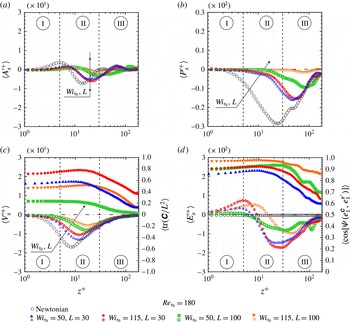
Figure 11. The open symbols show the normalized instantaneous streamwise work fluctuating terms against the normalized wall distance. The solid symbols in (c,d) show the profiles of $\langle \text{tr}(\unicode[STIX]{x1D63E})/L^{2}\rangle$ and $\langle \cos \unicode[STIX]{x1D6F9}(e_{1}^{\unicode[STIX]{x1D63E}},e_{1}^{\unicode[STIX]{x1D749}^{\prime }})\rangle$ across the channel half-width, respectively.

In the viscous sublayers of both the low and the high drag reduction regimes (figures 9 and 10, respectively), while $e_{2}^{\unicode[STIX]{x1D63E}}$ and $e_{1}^{\unicode[STIX]{x1D63F}}$ are almost orthogonal, there is an angle of ${\approx}45^{\circ }$ between $e_{3}^{\unicode[STIX]{x1D63E}}$ and $e_{1}^{\unicode[STIX]{x1D63F}}$ , as well as between $e_{1}^{\unicode[STIX]{x1D63E}}$ and $e_{1}^{\unicode[STIX]{x1D63F}}$ . Interestingly, $\unicode[STIX]{x1D6F9}(e_{1}^{\unicode[STIX]{x1D63E}},e_{1}^{\unicode[STIX]{x1D63F}})$ is maintained across the channel. In contrast, in the LDR scenario, both $\unicode[STIX]{x1D6F9}(e_{3}^{\unicode[STIX]{x1D63E}},e_{1}^{\unicode[STIX]{x1D63F}})$ and $\unicode[STIX]{x1D6F9}(e_{2}^{\unicode[STIX]{x1D63E}},e_{1}^{\unicode[STIX]{x1D63F}})$ become random as the wall distance increases. However, in the HDR regime, this tendency of chaotic alignment within the region III is attenuated, and, in consequence, $\langle \cos \unicode[STIX]{x1D6F9}(e_{3}^{\unicode[STIX]{x1D63E}},e_{1}^{\unicode[STIX]{x1D63F}})\rangle \approx 0.6$ and $\langle \cos \unicode[STIX]{x1D6F9}(e_{2}^{\unicode[STIX]{x1D63E}},e_{1}^{\unicode[STIX]{x1D63F}})\rangle \approx 0.25$ . Thus, as $Wi_{\unicode[STIX]{x1D70F}_{0}}$ and $L$ increase, the polymer becomes more exposed to the rate-of-strain tensor not only in regions I and II, but also in region III.

Near the wall, the polymer molecules exhibit a weak tendency to lie in the plane perpendicular to $\unicode[STIX]{x1D74E}$ since $\langle \cos \unicode[STIX]{x1D6F9}(e_{1}^{\unicode[STIX]{x1D63E}},\unicode[STIX]{x1D74E})\rangle$ and $\langle \cos \unicode[STIX]{x1D6F9}(e_{3}^{\unicode[STIX]{x1D63E}},\unicode[STIX]{x1D74E})\rangle$ are almost zero, as can be seen in figures 9 and 10. However, one can note that in this region, $\langle \cos \unicode[STIX]{x1D6F9}(e_{2}^{\unicode[STIX]{x1D63E}},\unicode[STIX]{x1D74E})\rangle \approx 1.0$ . This occurs because, near the wall, $e_{2}^{\unicode[STIX]{x1D63E}}$ is oriented along the $e_{y}$ direction (not shown here), as is $\unicode[STIX]{x1D74E}$ (see figures 7 and 8).

5.1 Global exchanges of energy

As pointed out in previous subsections, near-wall polymers are highly aligned with $\unicode[STIX]{x1D749}^{\prime }$ and, consequently, strongly exposed to flow stress fluctuations. The latter are responsible for the generation of intermittent quasi-streamwise vortices, which play a very important role in the momentum exchange as well as in the increase of the turbulent friction drag (see Kravchenko, Choi & Moin Reference Kravchenko, Choi and Moin1993). Hence, our tensorial and statistical analyses suggest that polymers primarily interact with these intermittent structures, exchanging energy with them. Aiming to characterize such energy exchanges, we consider the work fluctuation terms. These energy terms are that exclusively related to the fluctuating fields which appear in the right-hand side of the work fluctuation equation, which in turn is obtained by decomposing the variables of the momentum equation into mean flow ( $\overline{U}_{\unicode[STIX]{x1D6FC}}^{+}$ , $\overline{p}^{+}$ and $\overline{\unicode[STIX]{x1D6EF}}_{\unicode[STIX]{x1D6FC}j}^{+}$ ) and fluctuations ( ${u_{\unicode[STIX]{x1D6FC}}^{\prime }}^{+}$ , ${p^{\prime }}^{+}$ and ${\unicode[STIX]{x1D6EF}_{\unicode[STIX]{x1D6FC}j}^{\prime }}^{+}$ ), and then multiplying the resulting equation by the streamwise velocity fluctuations ( ${u_{\unicode[STIX]{x1D6FC}}^{\prime }}^{+}$ ). A detailed deduction of the work equations is provided in appendix A. The work terms exclusively linked with the fluctuating fields are then: ${E_{\unicode[STIX]{x1D6FC}}^{\prime }}^{+}=({u_{\unicode[STIX]{x1D6FC}}^{\prime }}^{+}(\unicode[STIX]{x2202}{\unicode[STIX]{x1D6EF}_{\unicode[STIX]{x1D6FC}j}^{\prime }}^{+}/\unicode[STIX]{x2202}x_{j}^{+}))$ , ${A_{\unicode[STIX]{x1D6FC}}^{\prime }}^{+}=[{-u_{\unicode[STIX]{x1D6FC}}^{\prime }}^{+}(\unicode[STIX]{x2202}({u_{\unicode[STIX]{x1D6FC}}^{\prime }}^{+}{u_{j}^{\prime }}^{+})/\unicode[STIX]{x2202}x_{j}^{+})]$ , ${P_{\unicode[STIX]{x1D6FC}}^{\prime }}^{+}=({-u_{\unicode[STIX]{x1D6FC}}^{\prime }}^{+}(\unicode[STIX]{x2202}{p^{\prime }}^{+}/\unicode[STIX]{x2202}x^{+}))$ and ${V_{\unicode[STIX]{x1D6FC}}^{\prime }}^{+}=[(\unicode[STIX]{x1D6FD}_{0}){u_{\unicode[STIX]{x1D6FC}}^{\prime }}^{+}(\unicode[STIX]{x2202}^{2}{u_{\unicode[STIX]{x1D6FC}}^{\prime }}^{+}/\unicode[STIX]{x2202}{x_{j}^{+}}^{2})]$ . Since the turbulent energy exchanges in the $x$ direction constitute more than $90\,\%$ of that considering the streamwise, the spanwise and the wall-normal directions, we analyse here only the streamwise work fluctuation terms ( $\unicode[STIX]{x1D6FC}=x$ ). Hence, the instantaneous polymer work term, ${E_{x}^{\prime }}^{+}$ , indicates the amount of energy stored ( ${E_{x}^{\prime }}^{+}<0$ ) or released ( ${E_{x}^{\prime }}^{+}>0$ ) by the polymers from the fluctuating velocity field in the streamwise direction, ${u_{x}^{\prime }}^{+}$ (the fluctuations are denoted by the superscript ‘ $\prime$ ’). The supplementary fluctuating work terms denote the advection, ${A_{x}^{\prime }}^{+}$ , the pressure redistribution, ${P_{x}^{\prime }}^{+}$ , and the viscous stress, ${V_{x}^{\prime }}^{+}$ . The sum ${A_{x}^{\prime }}^{+}+{P_{x}^{\prime }}^{+}+{V_{x}^{\prime }}^{+}$ is referred to as the Newtonian fluctuating work, ${N_{x}^{\prime }}^{+}$ .

Figure 12. The open symbols show the normalized instantaneous streamwise work fluctuating terms against the normalized wall distance. The solid symbols in (c,d) show the profiles of $\langle \text{tr}(\unicode[STIX]{x1D63E})/L^{2}\rangle$ and $\langle \cos \unicode[STIX]{x1D6F9}(e_{1}^{\unicode[STIX]{x1D63E}},e_{1}^{\unicode[STIX]{x1D749}^{\prime }})\rangle$ across the channel half-width, respectively.

In figures 11 and 12, the $x$ – $y$ plane average of the instantaneous streamwise work fluctuating terms against the normalized wall distance are considered. In addition, both $\langle \text{tr}(\unicode[STIX]{x1D63E})/L^{2}\rangle$ and $\langle \cos \unicode[STIX]{x1D6F9}(e_{1}^{\unicode[STIX]{x1D63E}},e_{1}^{\unicode[STIX]{x1D749}^{\prime }})\rangle$ are plotted. These quantities are denoted by the solid symbols in figures 11(d) and 11(f), respectively. Different levels of elasticity are considered in figure 11 fixing the Reynolds number, while the effects of $Re_{\unicode[STIX]{x1D70F}_{0}}$ are shown in figure 12 maintaining $Wi_{\unicode[STIX]{x1D70F}_{0}}=115$ and $L=100$ . Our lowest Reynolds number case ( $Re_{\unicode[STIX]{x1D70F}_{0}}=180$ ) and the seven viscoelastic flows detailed in table 1 are considered.

Very close to the wall (I), where the turbulent stresses are negligible, the work fluctuation terms are close to zero. The streamwise viscous work fluctuation (figures 11 c and 12 c) and the streamwise polymer work fluctuation (figures 11 d and 12 d) exhibit a different behaviour in the vicinity of the wall. For the less elastic case (blue open triangles), the former decreases from the wall to $z^{+}\approx 10$ , where its minimum value is located. The latter, one order of magnitude smaller than $V_{x}^{\prime }$ , increases throughout the viscous sublayer, reaching its peak magnitude at $z^{+}\approx 5$ . It is worth noting that both the inflexion point of $\langle {E_{x}^{\prime }}^{+}\rangle$ and the minimum value of $\langle {V_{x}^{\prime }}^{+}\rangle$ are located at the same wall distance for each case analysed here. Additionally, the maximum values of $\langle \text{tr}(\unicode[STIX]{x1D63E})/L^{2}\rangle$ (solid symbols in figures 11 c and 12 c) and $\langle \cos \unicode[STIX]{x1D6F9}(e_{1}^{\unicode[STIX]{x1D63E}},e_{1}^{\unicode[STIX]{x1D749}^{\prime }})\rangle$ (solid symbols in figures 11 d and 12 d), quantities which develop parallel profiles, are observed at the same location ( $z^{+}\approx 10$ for the less elastic case). Both the advection and pressure terms become less pronounced as elasticity increases, playing a less important role in the fluctuating energy budget under LDR flow conditions (figure 11). In the opposite trend, more significant values of $\langle {A_{x}^{\prime }}^{+}\rangle$ and $\langle {P_{x}^{\prime }}^{+}\rangle$ are observed at higher $Re_{\unicode[STIX]{x1D70F}_{0}}$ (figure 12).

The black arrows in figure 11 indicate that increasing elasticity makes $\langle {A_{x}^{\prime }}^{+}\rangle$ , $\langle {P_{x}^{\prime }}^{+}\rangle$ , and $\langle {V_{x}^{\prime }}^{+}\rangle$ close to zero. This effect of increasing elasticity is more pronounced in the viscous term and, consequently, in the Newtonian term ( ${A_{x}^{\prime }}^{+}+{P_{x}^{\prime }}^{+}+{V_{x}^{\prime }}^{+}$ ) of which the minimum value changes from $\langle {N_{x}^{\prime }}^{+}\rangle \approx 0.225$ for the Newtonian case to $\langle {N_{x}^{\prime }}^{+}\rangle \approx -0.07$ for the most elastic case (not shown). Furthermore, the minimum and the maximum values observed in figure 11 move away from the wall as $Wi_{\unicode[STIX]{x1D70F}_{0}}$ and $L$ increase. On the other hand, as indicated by the black arrows in figure 12, for a fixed elasticity, the magnitude of the energy budget terms increases with increasing Reynolds number.

Intermittent energy transfers may be hidden even by instantaneous spatial-averaging procedures. Further evidence regarding such energy transfers are provided by figure 13, which shows five different joint probability density functions (JPF) for the $x$ – $y$ planes related to the less elastic case and located at $z^{+}\approx 5.0$ , where $\langle {E_{x}^{\prime }}^{+}\rangle$ is a maximum, as well as that situated at $z^{+}\approx 50$ , where $\langle {E_{z}^{\prime }}^{+}\rangle$ is a minimum (not shown here). The black solid line represents the JPF of $E_{\unicode[STIX]{x1D6FC}}^{\prime }$ versus $u_{\unicode[STIX]{x1D6FC}}^{\prime }$ (where $\unicode[STIX]{x1D6FC}$ can denote either $x$ or  $z$ ), whereas the red solid line represents the JPF which considers the instantaneous streamwise polymer work fluctuation and the cosine of the angle between the first principal directions of $\unicode[STIX]{x1D63E}$ and $\unicode[STIX]{x1D749}^{\prime }$ . Similar JPFs are displayed in figure 14 for the Newtonian work fluctuation at the same $x$ – $y$ planes. The work fluctuation terms were normalized by their temporal root mean square spatially averaged over the corresponding $x$ – $y$ plane. In this figure, the most probable events are indicated by internal lines. Although only our less elastic fluid is treated in this figure, all the supplementary viscoelastic cases present qualitatively similar trends.

Figure 13. Joint probability density functions of instantaneous polymer work versus instantaneous velocity fluctuation for the $x$ – $y$ planes located at $z^{+}=5.0$ (a,b) and $z^{+}=50$ (c,d). Fluctuation terms are normalized by their temporal root mean square spatially averaged over the corresponding $x$ – $y$ plane.

Figure 14. Joint probability density functions of instantaneous Newtonian work versus instantaneous velocity fluctuation over the $x$ – $y$ planes located at $z^{+}=5.0$ (a,b) and $z^{+}=50$ (c,d). Fluctuation terms are normalized by their respective temporal root mean square spatially averaged over the corresponding $x$ – $y$ plane.

Firstly, with regard to figure 13(a), it is important to observe that the polymer molecules are allowed to coil ( $E_{x}^{\prime }>0$ ) and stretch ( $E_{x}^{\prime }<0$ ) within the near-wall region ( $z^{+}\approx 5.0$ ). At such a location, the polymer molecules are predominantly injecting energy into the flow ( $E_{x}^{\prime }>0$ ) and, as a consequence, increasing both the negative and the positive streamwise velocity fluctuations as well as the absolute value of $T_{x}^{\prime }$ (see figure 11). Moreover, this injection of energy is closely related (has a higher probability) to negative values of $u_{z}^{\prime }$ , as shown in figure 13(b). Interestingly, the red solid lines in figure 13(b) reveal that more pronounced polymer–turbulence exchanges of energy occur when the conformation tensor is predominantly oriented along the first principal direction of $\unicode[STIX]{x1D749}^{\prime }$ ( $\cos \unicode[STIX]{x1D6F9}(e_{1}^{\unicode[STIX]{x1D63E}},e_{1}^{\unicode[STIX]{x1D749}^{\prime }})\approx 1$ ), which reinforces the relevance of the alignment between $\unicode[STIX]{x1D63E}$ and $\unicode[STIX]{x1D749}^{\prime }$ for the polymer–turbulence exchange of energy.

Figure 13 also shows that at $z^{+}\approx 50$ , polymers primarily extract energy from the flow ( $E_{z}^{\prime }<0$ ), which preferentially occurs where $u_{x}^{\prime }<0$ (figure 13 c) and $u_{z}^{\prime }<0$ (figure 13 d). However, the suppression of ejection flows ( $u_{x}^{\prime }<0$ and $u_{z}^{\prime }>0$ ; Q2 region) is also a moderately likely event.

Comparing figures 13 and 14, it is interesting to note that in the very near-wall region, $E_{x}^{\prime }$ and $N_{x}^{\prime }$ tend to have opposite signs. Hence, at $z^{+}\approx 5$ , injection events are strongly related to $E_{x}^{\prime }>0$ and $N_{x}^{\prime }<0$ . Similarly, at $z^{+}\approx 50$ , the ejection and injection events are linked with $E_{z}^{\prime }<0$ and $N_{z}^{\prime }>0$ .

5.2 Elliptical and hyperbolic exchanges of energy

In order to better understand the polymer coil–stretch process from the energy perspective, we divide the flow into three different regions by using the $Q$ -criterion discussed in § 4.1. Instead of the usual approach, where a threshold is chosen to produce a Boolean picture of the flow, as in figure 3, for example, we adopt the $Q$ -criterion as a measure of the intensity of stretching/rotation activity, i.e. we plot the $Q$ field. To this end, $Q$ is normalized in order to produce values between 0 and 1 (Martins et al. Reference Martins, Pereira, Mompean, Thais and Thompson2016) and thus takes the form

Normalized values $0\leqslant Q_{norm}<0.5$ represent swirling-like or elliptical regions, whereas $0.5<Q_{norm}\leqslant 1$ indicates a non-swirling-like or hyperbolic region. A value of $Q_{norm}=0.5$ represents transition surfaces where the magnitudes of $\unicode[STIX]{x1D652}$ and $\unicode[STIX]{x1D63F}$ are equal. This normalized vortex identification criterion was applied to the centre $x{-}z$ plane (at $y=0.75\unicode[STIX]{x03C0}$ ) for all viscoelastic flows corresponding to $Re_{\unicode[STIX]{x1D70F}_{0}}=180$ , as shown in figure 15. The vortical regions (swirling-like) are shown in blue, while the extensional regions (non-swirling-like) are shown in red. Green indicates the transition regions, generally referred to as parabolic, where the intensities of the rotational and extensional motions are close to each other. The lines around vortical regions represent the intersections between the $x$ – $y$ plane and vortices with $Q=0.01$ (consequently, the lines surround the blue parts). These lines are black or white, which indicates polymer stretching ( $E_{x}^{\prime }<0$ ) or coiling ( $E_{x}^{\prime }>0$ ) in the streamwise direction, respectively.

Figure 15. Contour of normalized $Q$ -criterion,  $Q_{norm}$ . The lines around vortical regions (blue and green regions) represent intersections between the $x$ – $y$ plane and vortices with $Q=0.01$ . These lines are black or white, which indicates polymer stretching or coiling, respectively.

Analysing figure 15, we first notice that both the vortical and extensional motion are weakened by increasing elasticity. Hence, green regions are more frequent in the HDR cases (c,d). Furthermore, the lines indicate that the morphology of the vortices changes with an increase of $Wi_{\unicode[STIX]{x1D70F}_{0}}$ and/or $L$ , since their thicknesses and streamwise lengths increase, while they become more parallel to the wall, something also seen in figure 3. Concerning the polymer–vortex interactions, it is apparent that the lines around the elliptical parts are predominantly black. Such a result reveals that polymers essentially stretch in such a region, extracting energy from the vortices. In addition, we note that far from the wall, polymers also store a significant amount of energy from the hyperbolic regions, which are mostly surrounded by black lines as well (not shown for clarity).

The extraction of energy from the elliptical and hyperbolic structures by the polymer is further explored in figure 16, where the contours of the normalized $Q$ -criterion were applied to the centre $y$ – $z$ plane (at $x=4.0\unicode[STIX]{x03C0}$ ) for our less elastic case. The arrows in figure 16(a) indicate the direction and the sense of the vectors resulting from $u_{y}^{\prime }$ and $u_{z}^{\prime }$ , while those in figure 16(b) illustrate the direction and the sense of the vectors resulting from polymer force fluctuations ( $f_{\unicode[STIX]{x1D6FC}}^{\prime }=E_{\unicode[STIX]{x1D6FC}}^{\prime }/u_{\unicode[STIX]{x1D6FC}}^{\prime }$ ) in both the spanwise and wall-normal directions (the vector magnitudes are not considered in these figures). Comparing both of these figures, it is apparent that, fundamentally, the polymer forces oppose the vortical motion (blue regions) by imposing a counter-torque around such structures. However, it is important to stress that in the extensional structures (yellow and red regions) the polymer forces also oppose the fluctuating velocities. Similar results were obtained for the other case (not shown here).

Figure 16. Velocity (a) and polymer body force (b) fluctuation vectors on the $y$ – $z$ plane at $x=4.0\unicode[STIX]{x03C0}$ . Contours of the normalized $Q$ -criterion,  $Q_{norm}$ , are also overlaid, with blue regions indicating large swirling strength and red regions representing large extensional deformations.

The energy exchanges between the polymers and turbulent structures are highlighted by the open symbols in figures 17 and 18, where the $x$ – $y$ plane average of the streamwise polymer work fluctuations (a) and the streamwise Newtonian work fluctuations (b) are plotted against the wall distance for both the elliptical (c,d) and the hyperbolic (e,f) regions, separately. Additionally, a similar analysis is displayed for $\langle \cos \unicode[STIX]{x1D6F9}(e_{1}^{\unicode[STIX]{x1D63E}},e_{1}^{\unicode[STIX]{x1D749}^{\prime }})\rangle$ plotted against $z^{+}$ (solid symbols in figures a,c,e).

Figure 17. The open symbols show the normalized streamwise polymer (a,c,e) and Newtonian (b,d,f) work fluctuations against the wall ( $z^{+}$ ) distance considering the whole channel (a,b) as well as the elliptical (c,d) and hyperbolic (e,f) regions, separately. The solid symbols in (a,c,e) show the profile of $\langle \cos \unicode[STIX]{x1D6F9}(e_{1}^{\unicode[STIX]{x1D63E}},e_{1}^{\unicode[STIX]{x1D749}^{\prime }})\rangle$ against the wall distance, in the same three domains.

Figure 18. The open symbols show the normalized streamwise polymer (a,c,e) and Newtonian (b,d,f) work fluctuations against the wall ( $z^{+}$ ) distance considering the whole channel (a,b) as well as the elliptical (c,d) and hyperbolic (e,f) regions, separately. The solid symbols in (a,c,e) show the profile of $\langle \cos \unicode[STIX]{x1D6F9}(e_{1}^{\unicode[STIX]{x1D63E}},e_{1}^{\unicode[STIX]{x1D749}^{\prime }})\rangle$ against the wall distance, in the same three domains.

Considering the whole channel evaluated in figures 17(a,b) and 18(a,b) it is found that polymers essentially release energy within the viscous sublayer, since $\langle {E_{x}^{\prime }}^{+}(z^{+}<5)\rangle >0$ . In contrast, after reaching its maximum value at $z^{+}\approx 5.0$ , $\langle {E_{x}^{\prime }}^{+}\rangle$ becomes negative and reaches expressive negative values in region II ( $20\leqslant z^{+}\leqslant 30$ ). Negative values of $\langle {E_{x}^{\prime }}^{+}\rangle$ are also observed within region III. Hence, the polymers store turbulent energy in both regions II and III ( $E_{\unicode[STIX]{x1D6FC}}^{\prime }<0$ ), and release it into the viscous sublayer ( $E_{x}^{\prime }>0$ ) by coiling along the streamwise direction, which increases the streamwise velocity fluctuations (see figure 1 b).

Inside the elliptical and hyperbolic structures, the streamwise polymer work fluctuation profiles follow the same trends as those described for the whole channel. Polymers release energy to elliptical (figures 17 c and 18 c) and hyperbolic (figures 17 e and 18 e) parts located in the near-wall region (I), which had been previously extracted from such structures in regions II and III. These results corroborate those shown in figure 15. On the other hand, in the wall-normal direction as well as in the spanwise direction (not shown here), the polymer molecules predominantly store turbulent energy from the elliptical and hyperbolic structures by stretching in region III, which reinforces our remarks concerning figure 16. It is important to emphasize that the polymer–turbulence exchanges of energy are more pronounced in hyperbolic regions, especially in the streamwise direction. Lastly, regarding $\langle \cos \unicode[STIX]{x1D6F9}(e_{1}^{\unicode[STIX]{x1D63E}},e_{1}^{\unicode[STIX]{x1D749}^{\prime }})\rangle$ (solid symbols), the more significant alignments between $\unicode[STIX]{x1D63E}$ and $\unicode[STIX]{x1D749}^{\prime }$ are situated in the hyperbolic regions (figures 17 e and 18 e). These alignments decrease monotonically from the viscous sublayer to the centre of the channel.

More significant elastic and inertial effects are observed for $\langle {N_{x}^{\prime }}^{+}\rangle$ (figures 17 b and 18 b), which is essentially negative along $z^{+}$ and reaches its minimum value in the region II ( $z^{+}\approx 20$ ). This term is one order of magnitude greater than $\langle {E_{x}^{\prime }}^{+}\rangle$ and becomes close to zero as $Wi_{\unicode[STIX]{x1D70F}_{0}}$ and $L$ increase, and $Re_{\unicode[STIX]{x1D70F}_{0}}$ decreases. Within the elliptical region (figures 17 d and 18 d), no positive values of $\langle {N_{x}^{\prime }}^{+}\rangle$ are observed (figures 17 d and 18 d). However, in the hyperbolic regions (figures 17 f and 18 f), after achieving its minimum value, $\langle {N_{x}^{\prime }}^{+}\rangle$ increases and reaches a positive peak magnitude at $z^{+}\approx 70$ .

Concerning figures 17 and 18, it is also important to note that, for each viscoelastic case, the profiles given by the sum of the energy terms shown in figure 17(c,e), and in figure 18(c,e) at each $z^{+}$ are approximately equal to those displayed in figures 17(a) and 18(a), respectively, which is also valid for figures 17(b,d,f) and 18(b,d,f). Such a result indicates that the amount of energy exchanged between the polymers and turbulence in the parabolic regions is negligible compared to that occurring in elliptical or hyperbolic regions.

Figure 19. The three-dimensional structures represent the isosurfaces of hyperbolic regions defined as a negative value of the second invariant of the velocity gradient tensor, $\unicode[STIX]{x1D735}\boldsymbol{u}$ . The colours indicate polymer stretching, $\text{tr}(\unicode[STIX]{x1D63E})/L^{2}$ .

In order to illustrate the role played by the addition of a polymer in the hyperbolic structures of the domain, consider the hyperbolic counterpart of figure 3. Since the magnitude of the second invariant of the velocity gradient is not altered when one interchanges the Euclidean norms of $\unicode[STIX]{x1D63F}$ and $\unicode[STIX]{x1D652}$ , a negative value of $Q$ with the same magnitude as the ones depicted in figure 3 would give the hyperbolic structure an intensity corresponding to the elliptical structure intensity of that figure, as measured by $Q$ . In this connection, what is seen in figure 19 is a distribution over the domain of hyperbolic structures corresponding to: $Q=-0.7$ for the Newtonian (figure 19 a); $Q=-0.7$ for the viscoelastic case with $Wi_{\unicode[STIX]{x1D70F}_{0}}=50$ , $L=30$ (figure 19 b); $Q=-0.7$ for the viscoelastic with $Wi_{\unicode[STIX]{x1D70F}_{0}}=115$ , $L=30$ (figure 19 c); $Q=-0.7$ for the viscoelastic case with $Wi_{\unicode[STIX]{x1D70F}_{0}}=50$ , $L=100$ (figure 19 d); and $Q=-0.1$ for the viscoelastic case with $Wi_{\unicode[STIX]{x1D70F}_{0}}=115$ , $L=100$ (figure 19 e). A direct comparison between figures 3 and 19 shows a remarkable similarity in the intensity of the structures. Although there are clear differences in the morphology of the corresponding hyperbolic structures, figure 19 shows that these turbulent entities are also weakened by the action of the polymer. As the elastic character of the polymer becomes more prominent, the hyperbolic structures are reduced in intensity and size in a quite similar fashion to what happened with the elliptical structures displayed in figure 3. We can deduce that the polymer molecules interact with the turbulence, damping the elliptical and hyperbolic turbulent structures and leading to a tendency of a dominant parabolic character in the flow domain.

Figure 20. Sketch of the polymer-induced drag reduction mechanism.