3.1. Decomposition of wall-attached structures

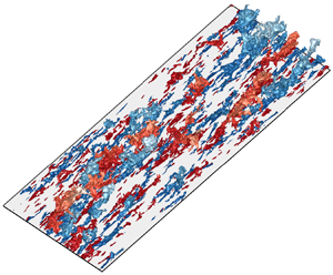
First, we decompose the wall-attached structures of $u$ in order to extract the self-similar structures. Figure 1 shows the isosurfaces of wall-attached structures ($y_{min}^+ \approx 0$) identified in all three flows. Here, light to dark shading indicates an increase in the wall-normal location. As seen, we can observe the coexisting streaky structures over a wide range of $l_y$ distributed over the surface. A noteworthy feature is that very tall structures with heights approaching $\delta$ are more evident in internal flows (figure 1$b$,$c$) compared with TBL (figure 1$a$). These large structures meander in the spanwise direction (Hutchins & Marusic Reference Hutchins and Marusic2007) and appear with the streamwise length over $10\delta$ in internal flows (Monty et al. Reference Monty, Stewart, Williams and Chong2007, Reference Monty, Hutchins, Ng, Marusic and Chong2009). Such a difference in very long structures may imply that we need to filter out those structures to examine the self-similar features of energy-containing motions in the logarithmic region.

Figure 1. Isosurfaces of wall-attached structures in an instantaneous flow field: ($a$) TBL; ($b$) channel; and ($c$) pipe. Red and blue isosurfaces indicate positive and negative streamwise velocity fluctuations, respectively. Light to dark shading indicates an increase in $y/\delta$.

To quantify the geometrical features of wall-attached structures, the joint probability density functions of the sizes of the identified structures are plotted in figure 2. Here, the shaded, red line and blue line contours denote the datasets of the TBL, channel and pipe flows, respectively. In general, the length ($l_x$) and width ($l_z$) of the structures increase with increasing heights ($l_y$) in all three flows. Interestingly, the distributions of $l_x$ and $l_z$ show a reasonably good collapse over a wide range of $l_y$ except for $l_y \approx O(\delta )$. This result indicates that the geometric features of the wall-attached $u$ structures in the inner region are presumably universal in canonical wall turbulence. On the other hand, there are very large-scale structures with $l_y \approx O(\delta )$, and some with $l_y \approx 2\delta$, in internal flows (red and blue line contours), which is consistent with the largest clusters of ejections or sweeps in channel flows (Lozano-Durán et al. Reference Lozano-Durán, Flores and Jiménez2012). The sizes of these structures are analogous to those of very large-scale motions (Kim & Adrian Reference Kim and Adrian1999) or global modes (del Álamo et al. Reference del Álamo, Jiménez, Zandonade and Moser2004) reported in internal flows. In TBL, very tall structures ($l_y \approx O(\delta )$) are associated with superstructures (Hutchins & Marusic Reference Hutchins and Marusic2007) because $l_x$ extends over $6\delta$ (see figure 1$a$) and they are physically attached to the wall (i.e. footprints in the near-wall region). Recent studies (Hwang & Sung Reference Hwang and Sung2018; Baars & Marusic Reference Baars and Marusic2020a; Yoon et al. Reference Yoon, Hwang, Yang and Sung2020) have reported that tall wall-attached structures are non-geometrically similar (or non-self-similar). In other words, this may reflect the fact that the statistical characteristics of these motions are non-universal and can be directly affected by the flow geometry. Hence, we need to filter out tall wall-attached structures in order to analyse the existence of self-similar features in the logarithmic layer (Hwang & Sung Reference Hwang and Sung2018; Baars & Marusic Reference Baars and Marusic2020a).

Figure 2. ($a$,$b$) Joint probability density functions of the logarithms of the streamwise length ($l_x$) and spanwise width ($l_z$) of wall-attached structures with respect to their wall-normal heights ($l_y$). Here, the shaded, red line and blue line contours indicate the datasets of the TBL, channel and pipe, respectively. Contour levels are logarithmically distributed.

Figure 3 presents the variation of the mean streamwise length $\langle l_x \rangle$ and the mean spanwise width $\langle l_z \rangle$ at a given $l_y$. The growth rates of $\langle l_x \rangle$ and $\langle l_z \rangle$ with respect to $l_y$ are comparable in all three flows. In figure 3($b$), we can see the linear relationship $\langle l_z \rangle \sim l_y$ over $l_y^+ > 3Re_{\tau }^{1/2}$. In contrast, $\langle l_x \rangle$ shows a power-law behaviour (i.e. $\langle l_x \rangle \sim l_y^{0.74}$) over $3Re_{\tau }^{1/2} < {l_y}^+ < 0.6\delta ^+$ (figure 3$a$) in all three flows. For $l_y^+ \ge 0.6\delta ^+$, the distribution of $\langle l_x \rangle$ starts to deviate away from the power law ($\langle l_x \rangle \sim l_y^{0.74}$). Although there is no linear relationship for the wall-attached $u$ structures over $3Re_{\tau }^{1/2} \le l_y^+ < 0.6\delta ^+$ in figure 3($a$), the sizes of the structures are scaled with $l_y$ and show a good agreement regardless of flow geometry. This result supports the supposition that the wall-attached structures in this range may share similar features. Moreover, the mean length $\langle l_x \rangle$ is approximately $3\delta$ at the upper limit $l_y^+ = 0.6\delta ^+$, which is consistent with the criteria to distinguish between large-scale and very large-scale motions (Guala et al. Reference Guala, Hommema and Adrian2006; Balakumar & Adrian Reference Balakumar and Adrian2007; Wu, Baltzer & Adrian Reference Wu, Baltzer and Adrian2012; Hwang, Lee & Sung Reference Hwang, Lee and Sung2016a; Hwang et al. Reference Hwang, Lee, Sung and Zaki2016b). This limit also corresponds to the criteria that distinguish self-similar structures from non-self-similar ones in an adverse-pressure-gradient TBL (Yoon et al. Reference Yoon, Hwang, Yang and Sung2020). Notably, $l_y^+ = 0.6\delta ^+$ is larger than the wall-normal location of the outer peak in the one-dimensional premultiplied spectra of $u$, which characterises very large-scale motions or superstructures. Given that $l_y$ is measured from the bounding box of each structure, the wall-parallel area of each structure is close to zero as $y$ approaches $l_y$, and they have the maximum wall-parallel area at $y < l_y$.

Figure 3. Mean length ($\langle l_x \rangle$) and width ($\langle l_z \rangle$) of wall-attached structures as a function of $l_y$. In panel ($a$), the dashed line is $\langle l_x \rangle \sim l_y^{0.74}$ (Hwang & Sung Reference Hwang and Sung2018). In panel ($b$), the solid line corresponds to $\langle l_z \rangle \approx l_y$.

Hence, the wall-attached $u$ structures can be classified into three components in terms of $l_y$: buffer-layer, self-similar and non-self-similar structures defined as $l_y^+ < 3Re_{\tau }^{1/2}$, $3Re_{\tau }^{1/2} \le l_y^+ < 0.6\delta ^+$ and $0.6\delta \le l_y^+$, respectively. Here, the lower bound ($= 3Re_{\tau }^{1/2}$ of self-similar structures corresponds to that of the logarithmic region in Marusic et al. (Reference Marusic, Monty, Hultmark and Smits2013) and Hwang & Sung (Reference Hwang and Sung2019), which is a mesolayer scaling (Afzal Reference Afzal1982; Wei et al. Reference Wei, Fife, Klewicki and McMurtry2005). Given that the viscous effect may affect the coherent motions in the logarithmic region (Hwang Reference Hwang2016), the bound $3Re_{\tau }^{1/2}$ is used in the present study. The present Reynolds number is $Re_{\tau } \approx 1000$ in which, in turn, the lower bound is approximately 100 wall units (i.e. $3Re_{\tau }^{1/2} \approx 100$), that is, a classical scaling for the lower bound of the logarithmic region (Perry & Chong Reference Perry and Chong1982). Since we focus on the logarithmic region where $y^+ > 100$, the variation of the lower bounds does not have a major impact on our conclusions.

The power law ($\langle l_x \rangle \sim l_y^{0.74}$) for the WASS could be attributed to the low Reynolds number of the present data. At $Re_{\tau } \approx 3000$, the linear relationship ($\langle l_x \rangle \sim l_y$) was observed for $l_y^+ > 400$ in a turbulent pipe flow (Hwang & Sung Reference Hwang and Sung2019). Given $\langle l_z \rangle \sim l_y$, the wall-attached structures with $3Re_{\tau }^{1/2} \le l_y^+ < 0.6\delta ^+$ follow $\langle l_x \rangle l_y \sim \langle l_z \rangle ^{1.74}$, which is roughly quadratic. This behaviour is consistent with the scaling of the two-dimensional spectra of $u$ at $Re_{\tau } < 2000$ (del Álamo et al. Reference del Álamo, Jiménez, Zandonade and Moser2004) in which the energetic ridges of the spectra are aligned along $\lambda _x y \sim \lambda _z^2$ in the logarithmic region. Chandran et al. (Reference Chandran, Baidya, Monty and Marusic2017) reported that the two-dimensional spectra at low Reynolds number follow $\lambda _x y \sim \lambda _z^2$ whereas the larger scales tend to exhibit the linear law ($\lambda _x \sim \lambda _z$) at high Reynolds numbers ($Re_{\tau } = 26\,000$). Although we defined the length scales of wall-attached structures based on the sizes ($l_x, l_y$ and $l_z$) of the bounding box of each structure, this result supports the inference that $l_x, l_y$ and $l_z$ can be used to describe the characteristic length scales of the energetic motions in the logarithmic region. It should be noted that these scales are measured from the physically connected volumes of intense $u$, which consist of the energy contributions from a wide range of scales (or wavelengths). In § 3.2, the two-dimensional energy spectra are examined to elucidate the wavelength scales contained within the WASS.

To test the reliability of the present decomposition, we compute the streamwise turbulence intensity distributed among the three components of wall-attached $u$ structures. The streamwise velocity fluctuations associated with each component ($u_i$) can be conditionally sampled based on the bounded volume of each object,

(3.1)\begin{equation} \left. \begin{gathered} u_{b}(\boldsymbol{x}) = \left\{ \begin{array}{ll} u(\boldsymbol{x}), & \text{if}\ \boldsymbol{x} \in \varOmega_b, \\ 0, & \text{otherwise}, \end{array} \right.\\ u_{ws}(\boldsymbol{x}) = \left\{ \begin{array}{ll} u(\boldsymbol{x}), & \text{if}\ \boldsymbol{x} \in \varOmega_{ws}, \\ 0, & \text{otherwise}, \end{array} \right.\\ u_{wn}(\boldsymbol{x}) = \left\{ \begin{array}{ll} u(\boldsymbol{x}), & \text{if}\ \boldsymbol{x} \in \varOmega_{ws}, \\ 0, & \text{otherwise}, \end{array} \right. \end{gathered} \right\} \end{equation}

where $\varOmega _i$ denotes the positions of all contiguous points of each object. The subscripts $i$ b, ws and wn refer to wall-attached buffer-layer ($l_y^+ < 3Re_{\tau }^{1/2}$), self-similar ($3Re_{\tau }^{1/2} \le l_y^+ < 0.6\delta ^+$) and non-self-similar structures ($0.6\delta \le l_y^+$), respectively. This classification yields a computation of the streamwise turbulence intensity corresponding to the specific structure. For example, the streamwise turbulence intensity carried by WASS $\langle uu \rangle _{ws}$ can be obtained through the ensemble average of $u_{ws}u_{ws}$ at a given wall-normal position.

Figure 4 shows the wall-normal distributions of the streamwise turbulence intensity carried by the specific motion. Notably, we can observe the presence of the near-wall peak in all streamwise turbulence intensities because the identified structures physically adhere to the wall. Hence, the near-wall part (or footprint) of each object is related to the near-wall streaks (Kline et al. Reference Kline, Reynolds, Schraub and Runstadler1967), reflecting that the identified structures could be responsible for the near-wall turbulence. However, this is beyond the scope of the present work, which focuses on the logarithmic region. The total streamwise turbulence intensity ($\langle uu \rangle _{w}$) contained within all three components is shown in figure 4($a$). Here, $\langle uu \rangle _{w}$ is obtained using the streamwise velocity fluctuations within the wall-attached structures ($= u_b + u_{ws} + u_{wn}$). As seen, there is a complete collapse of the wall-normal profiles of $\langle uu \rangle _{w}$ in internal flows across the wall-normal direction. In contrast, the $\langle uu \rangle _{w}$ of TBL shows a discrepancy above the logarithmic region ($y^+ > 100$). This discrepancy occurs at a lower wall-normal location compared with the results of Monty et al. (Reference Monty, Hutchins, Ng, Marusic and Chong2009), who reported that the difference in $\langle uu \rangle$ between internal and external flows appears at $y > 0.5\delta$. Given that $\langle uu \rangle _{w}$ represents the collective contributions of the wall-attached structures, the deviation in figure 4($a$) is due to the structures with $l_y^+ > 100$, which include WASS and wall-attached non-self-similar structures (WANS). The weak-$u$ region ($|u| < u_{rms}$) also significantly contributes to the total streamwise turbulence intensity because this region has a larger area fraction than the intense $u$ region (2.1). The area fraction of the wall-attached $u$ structures is only 6–7 % in the logarithmic region. However, the contribution of the wall-attached $u$ structures to the total turbulence intensity is approximately 40 %, which is comparable to that of the weak-$u$ region. This may lead to the absence of the logarithmic variation in the total streamwise turbulence intensity at the present $Re_{\tau }$ (Hwang & Sung Reference Hwang and Sung2018).

Figure 4. Wall-normal profiles of streamwise turbulence intensity carried by wall-attached structures: ($a$) $\langle uu \rangle _w^+$; ($b$) $\langle uu \rangle _{ws}^+$; ($c$) $\langle uu \rangle _{b}^+$; and ($d$) $\langle uu \rangle _{wn}^+$. In panel ($b$), the solid line denotes a logarithmic variation corresponding to $\langle uu \rangle _{ws}^+ = 0.4 - 0.37\ln (y/\delta )$.

Figure 4($b$) displays the streamwise turbulence intensity carried by the WASS ($\langle uu \rangle _{ws}$). In all three flows, the profiles of $\langle uu \rangle _{ws}$ show good agreement (figure 4$b$), indicating that the WASS are independent of the flow geometry (Perry et al. Reference Perry, Henbest and Chong1986). In addition, there is a logarithmic variation of up to $y = 0.3\delta$ in all three flows, reminiscent of Townsend's attached eddies. In figure 4($c$), the streamwise turbulence intensity of the buffer-layer structures $\langle uu \rangle _b$ also exhibits a reasonable match in all three flows. Hence, the similarity in the streamwise turbulence intensity in all three flows (figure 4$b$,$c$) suggests that geometrical differences are negligible in the near-wall region.

In contrast, figure 4($d$) shows that the $\langle uu \rangle _{wn}$ of internal flows appears to be larger than that of TBL in the outer region. This supports that the discrepancy in $\langle uu \rangle _w$ over the logarithmic region (figure 4$a$) originates from the non-self-similar nature of very tall structures (i.e. WANS), which extend from the near-wall region to the core region of internal flows. In addition, comparing pipe and channel data, $\langle uu \rangle _{wn}$ of the channel flow is larger than that of the pipe flow in the logarithmic region. This might be attributable to a larger population of very long $u$ streaks in the channel flow (Lee et al. Reference Lee, Ahn and Sung2015). Owing to pipe curvature, the sizes of very large structures could be restricted in pipe flows; this leads to the dominant contributions of large scales in the channel flow (Hwang et al. Reference Hwang, Lee and Sung2016a; Han et al. Reference Han, Hwang, Yoon, Ahn and Sung2019).

It is worth mentioning that the magnitude of the slope of the logarithmic variation in figure 4($b$) is 0.37, which is lower than the Townsend–Perry constant reported in previous studies (1.26 by Marusic et al. (Reference Marusic, Monty, Hultmark and Smits2013), 0.98 by Baars & Marusic (Reference Baars and Marusic2020b) and 0.8–1.0 by Hu et al. (Reference Hu, Yang and Zheng2020)). This is due to the decomposition method used here in which $u_{ws}$ is zero at the outside of the identified structures (3.1). As a result, the magnitude of $\langle uu \rangle _{ws}$ decreases, which leads to a lower slope of the logarithmic variation. However, we primarily focus on the presence of the logarithmic variation in streamwise turbulence intensity and the collapse of the corresponding profiles in all three flows obtained from the classification of wall-attached $u$ structures in terms of height. The presence of the logarithmic variation could be a consequence of the spatial organisation (self-similarity and distributions) of WASS in the context of the AEH.

The present decomposition method filters wall-attached structures that are geometrically self-similar. By filtering out the contributions of WANS in the logarithmic region, we can analyse the spectral signature of self-similar coherent motions. In the next section, the two-dimensional energy spectra of $u_{ws}$ are examined by focusing on the self-similar scaling laws proposed by Perry and coworkers (Perry & Abell Reference Perry and Abell1977; Perry & Chong Reference Perry and Chong1982; Perry et al. Reference Perry, Henbest and Chong1986), and on the energy distribution across the streamwise and spanwise wavelengths ($\lambda _x$ and $\lambda _z$) in the logarithmic region.

3.2. Two-dimensional spectra of WASS

The contribution of coherent motions ingrained within WASS to the streamwise variance is explored by computing the two-dimensional spectrum. The premultiplied two-dimensional spectrum of $u_{ws}$, $\varPhi ^{2D}$, is defined as

(3.2)\begin{equation} \varPhi^{2D}(k_x, k_z, y) = k_x k_z \langle \hat{u}_{ws}(k_x, k_z, y) \hat{u}^{*}_{ws}(k_x, k_z, y) \rangle, \end{equation}

where $k_x (= 2{\rm \pi} /\lambda _x)$ and $k_z (= 2{\rm \pi} /\lambda _z)$ are the streamwise and spanwise wavenumbers, $\hat {u}_{ws}$ indicates the Fourier coefficient of $u_{ws}$ and the asterisk denotes a complex conjugate. The streamwise variance of WASS ($\langle uu \rangle _{ws}$) is the integral of the corresponding two-dimensional spectrum over the wall-parallel wavenumbers. Notably, $l_x$ and $l_z$ of the identified structures, measured from the bounding box, do not necessarily represent the characteristic scales at a given wall-parallel plane ($y < l_y$) because the structures are inclined with respect to the wall and meander in the spanwise direction. Given that $u_{ws}$ represents the conditionally sampled $u$ which are contained within the WASS with $y \le l_y < 0.6\delta$, $\varPhi ^{2D}$ could provide the energy distributions from the collective contribution of WASS. In other words, although the ranges of the corresponding physical length and width are 5–6$y < \langle l_x \rangle < 2\delta$ and $y < \langle l_z \rangle < 0.6\delta$ (figure 3), the energy in $\varPhi ^{2D}$ is distributed across a wide range of wavelengths. This also supports the inference that the structures identified in the physical space consist of a broad range of turbulent motions related to the concept of nested hierarchies (Hwang & Sung Reference Hwang and Sung2018). Here, the energy contained in the very long and wide wavelengths ($\lambda _x > 6\delta$ and $\lambda _z > \delta$), which correspond to global modes (del Álamo et al. Reference del Álamo, Jiménez, Zandonade and Moser2004; Jiménez & Hoyas Reference Jiménez and Hoyas2008), is negligible because the velocity fluctuations associated with WANS are subtracted. Hence, we can expect that the energy distribution demonstrates the spectral signature of self-similar coherent motions. The effect of the threshold $\alpha$ was examined and the results reported in this section remained qualitatively unchanged (see the Appendix).

Figure 5 shows the contours of $\varPhi ^{2D}$ at various wall-normal positions located in the logarithmic region ($y^+ = 100, 110, 120$ and $130$) for all three flows. Here, $\varPhi ^{2D}$ as a function of the wavelengths scaled with $y$ and $\delta$ is plotted in panels (a,c,e) and (b,d,f), respectively. In general, all three flows show that $\varPhi ^{2D}$ scales reasonably well with $y$ in the range $y < \lambda _x < 10y$ (figure 5$a{,}c{,}e$) and with $\delta$ in the range $\lambda _x > \delta$ (figure 5$b{,}d{,}f$). To further examine the spectral behaviour, the bounds of the constant energy distribution are denoted by the green lines. Here, the dashed and solid lines represent a square root $\lambda _x \sim \lambda _z^2$ and linear relationship $\lambda _x \sim \lambda _z$, respectively. The contours of $\varPhi ^{2D}$ in figure 5($a{,}c{,}e$) are bounded by $\lambda _x \sim \lambda _z^2$ over the range $y < \lambda _x < 10y$. This is consistent with the results of the two-dimensional spectra of $u$, which include all coexisting motions, at low $Re_{\tau } \approx O(10^3)$ in the works of del Álamo et al. (Reference del Álamo, Jiménez, Zandonade and Moser2004) and Chandran et al. (Reference Chandran, Baidya, Monty and Marusic2017). According to del Álamo et al. (Reference del Álamo, Jiménez, Zandonade and Moser2004) and Chandran et al. (Reference Chandran, Baidya, Monty and Marusic2017), the linear relationship was absent in the large-scale range at low $Re_{\tau }$. In the large-scale range ($\lambda _x > 12y$), however, $\varPhi ^{2D}$ are roughly aligned along $\lambda _x \sim \lambda _z$ (solid lines), which is an indicator of self-similarity. Moreover, the contour lines of $\varPhi ^{2D}$ collapse reasonably well along the lower bound $\lambda _x = 10\lambda _z$ with both $y$ and $\delta$ scaling in this large-scale range, reflecting the overlap arguments of self-similar energy-containing motions (Perry & Abell Reference Perry and Abell1977; Perry & Chong Reference Perry and Chong1982; Perry et al. Reference Perry, Henbest and Chong1986). This result also supports the existence of Townsend's attached eddies, even in low $Re_{\tau }$ (Hwang & Sung Reference Hwang and Sung2018), and further reveals that the WASS, defined in physical space, is tightly connected to the spectral signatures of the AEH in the framework used by Perry and coworkers.

Figure 5. Premultiplied two-dimensional energy spectra $\varPhi ^{2D}$ across the logarithmic region ($y^+ = 100, 110, 120$ and $130$): ($a{,}b$) TBL; ($c{,}d$) channel; and ($e{,}f$) pipe. Light to dark shading indicates an increase in $y$. The contour level is $0.4$ times each of the maxima. Here $\varPhi ^{2D}$ is plotted as a function of the wall-parallel wavelengths ($\lambda _x$ and $\lambda _z$) normalised by $y$ ($a$,$c$,$e$) and $\delta$ ($b$,$d$,$f$). The green dashed and solid lines denote $\lambda _x \sim \lambda _z^2$ and $\lambda _x \sim \lambda _z$, respectively. The vertical dashed line indicates $\lambda _x = 12y$.

It is worth noting that the linear relationship of the upper bound in the large-scale range ($\lambda _x \approx 2\text{--}3\lambda _z$) seems to appear over a small range owing to low $Re_{\tau }$. At high $Re_{\tau } = O(10^4)$, the upper and lower bounds of the two-dimensional spectra follow the linear relationship in the large-scale range (Chandran et al. Reference Chandran, Baidya, Monty and Marusic2017; Deshpande et al. Reference Deshpande, Chandran, Monty and Marusic2020). As shown in figure 5($b{,}d{,}f$), the contour lines of $\varPhi ^{2D}$ in the large scale range are aligned along the horizontal line $\lambda _z \approx 0.8\delta$. Given that the growth of energy-containing motions can be restricted as their heights reach $\delta$, there may not be enough space to maintain large-scale self-similar motions at the present Reynolds number. According to the AEH, self-similar energy-containing motions fill in the scale separation between $\nu /u_{\tau }$ and $\delta$. At high Reynolds numbers, it can be conjectured that the contours of $\varPhi ^{2D}$ in the outer scaling would move to the bottom left-hand corner and lead to a clear upper bound that follows the linear behaviour. This upper bound may lie below $\lambda _x = \lambda _z$ (i.e. a higher slope than unity) due to the inclination nature of wall-attached $u$ structures (figures 1 and 3$a$). In other words, it may imply that self-similar behaviour can be observed when large-scale energy-containing motions have a high aspect ratio $\lambda _x/\lambda _z$ (Chandran et al. Reference Chandran, Baidya, Monty and Marusic2017).

As discussed, the linear behaviour of the lower bound ($\lambda _x = 10\lambda _z$) is observed in the large-scale range where $\lambda _x > 12y$ (denoted by vertical dashed lines in figure 5$a{,}c{,}e$). Such a feature is found in all three flows indicative of the universality of the self-similar nature of the large scales contained within WASS. In addition, $\lambda _x > 12y$ is consistent with the lower limit of the $k_x^{-1}$ region in channel flows (Hwang Reference Hwang2015), and is close to the inner-scaling limit ($\lambda _x = 14y$) of self-similar motions in TBLs over a wide range of $Re_{\tau }$ (Baars et al. Reference Baars, Hutchins and Marusic2017). A recent study by Deshpande et al. (Reference Deshpande, Chandran, Monty and Marusic2020) also found the existence of linear behaviour in two-dimensional cross-spectra of wall-coherent $u$ motions over a similar range (i.e. $\lambda _x > 15y$). This shows that the WASS identified in the present study is directly related to the self-similar behaviour in the wavenumber space. In § 3.3, the one-dimensional spectra of WASS are examined to observe the presence of the $k_x^{-1}$ region over a similar large-scale range ($\lambda _x > 12y$), which was absent in the aforementioned study.

It is worth mentioning that $u_{ws}$ could demarcate the rapid change in the raw $u$. Wall-attached $u$ structures are composed of multiple UMZs (Hwang & Sung Reference Hwang and Sung2018). Given that the UMZs are demarcated by a thin shear layer or large velocity gradient (Meinhart & Adrian Reference Meinhart and Adrian1995; Adrian et al. Reference Adrian, Meinhart and Tomkins2000), the boundaries of the identified structures may be one of the internal shear layers where the streamwise momentum exhibits a sharp change in the velocity. We can observe a rapid variation of the raw velocity signals near the edges of the identified structure; see figure 9 in Hwang & Sung (Reference Hwang and Sung2018). This result supports the inference that $u_{ws}$ can retain the spectral characteristics of the raw $u$ signals even if we artificially impose zero velocity outside of the identified structures. Srinath et al. (Reference Srinath, Vassilicos, Cuvier, Laval, Stanislas and Foucaut2018) also reported that binary representation of the negative-$u$ structures could preserve the spectral information of raw $u$ because of large changes in $u$ at the edges of the identified structures.

To further explore the energy contribution from self-similar motions, the spectral ridge of $\varPhi ^{2D}$ is plotted in figure 6. Here, the spectral ridge is determined by identifying $\lambda _z$ corresponding to the maximum value of $\varPhi ^{2D}$ at a given $\lambda _x$. Hence, figure 6 represents the length scale ($\lambda _x$ and $\lambda _z$) relationship of the energetic motions. All of the spectral ridges are found to agree reasonably well over a wide range of scales. We can observe two growth rates: one with the power-law behaviour $\lambda _x \sim \lambda _z^2$ (dashed green line), and one with the linear relationship $\lambda _x \sim \lambda _z$ (solid green line) at relatively large scales. In addition, the transition of the ridges from the power law to the linear law appears at $\lambda _x = 12y$. This result is consistent with the variation of the lower and upper bounds of $\varPhi ^{2D}$ found in figure 5 and reflects that the dimensions of the energetic motions behave in an analogous manner to the wavelength relationship of the bounds (i.e. self-similarity). It is noted that the spectral ridges flatten for $\lambda _x > 3\text{--}4\delta$ because at this very long $\lambda _x$ the spanwise wavelength $\lambda _z$ reaches $\delta$, and the growth of $\lambda _z$ is restricted. A similar spectral trend was observed in Chandran et al. (Reference Chandran, Baidya, Monty and Marusic2017) and Deshpande et al. (Reference Deshpande, Chandran, Monty and Marusic2020). Given that the wall-attached $u$ structures follow $\langle l_z \rangle \approx l_y$ (figure 3$b$), it may reflect the saturation in their spanwise growth. Although the motions related to these scales are non-self-similar, the energy contribution from the range $\lambda _x > 3\text{--}4\delta$ and $\lambda _z > 0.8\delta$ is negligible, as shown in figure 5, since $\varPhi ^{2D}$ is obtained from $u_{ws}$ (3.1).

Figure 6. Energetic ridges of the premultiplied two-dimensional energy spectra $\varPhi ^{2D}$ at $y^+ = 120$. Here, the positions of the ridges are obtained by identifying $\lambda _z$ of the maximum $\varPhi$ at a given $\lambda _x$. The dashed and solid green lines represent the power-law ($\lambda _x = (4\lambda _z)^2$) and linear relationships ($\lambda _x = 4\lambda _z$), respectively. In panel ($a$), the inset shows the lin–lin plot of the ridge scale ratio $\lambda _x / \lambda _z$ for the TBL and channel data. The horizontal dashed line denotes a constant ratio $\lambda _x / \lambda _z \approx 4.$.

In figure 6, the linear behaviour seems to follow $\lambda _x \approx 4\lambda _z$ over the range $12y < \lambda _x < 3\text{--}4\delta$. Here, the inset shows the ridge scale ratio $\lambda _x / \lambda _z$ for the TBL and channel data. The data over this range are not very far from the dashed line ($\lambda _x / \lambda _z \approx 4$). Hence, the range of the self-similar energetic motions ingrained in WASS can be expressed by

(3.3a)\begin{gather} 12y < \lambda_x < 3\text{--}4\delta, \end{gather}

(3.3b)\begin{gather}3y < \lambda_z < 0.8\text{--}1\delta. \end{gather}

Here, the upper limit for the streamwise wavelength in (3.3a) is $3\text{--}4\delta$, similar to that of the criteria that distinguishes large-scale motions and very large-scale motions (Guala et al. Reference Guala, Hommema and Adrian2006; Balakumar & Adrian Reference Balakumar and Adrian2007; Wu et al. Reference Wu, Baltzer and Adrian2012; Hwang et al. Reference Hwang, Lee and Sung2016a). In particular, the upper limit of the TBL ($\approx 3\delta$) is relatively smaller than that of the internal flows ($\approx 4\delta$), which may be related to the dominant contribution of very long scales in internal flows (Monty et al. Reference Monty, Hutchins, Ng, Marusic and Chong2009). Given that the contours of $\varPhi ^{2D}$ are restricted to below $\lambda _x \approx 3\text{--}4\delta$ in figure 5, this result also supports that $\varPhi ^{2D}$ is composed of the contribution from the turbulence motions that include large-scale motions and relatively smaller motions.

It is worth mentioning that a similar linear relationship of wall-attached $u$ structures was found by Hwang & Sung (Reference Hwang and Sung2019), who showed that the physical length and width of WASS exhibit $\langle l_x \rangle = 4\langle l_z \rangle$ in a higher Reynolds number pipe flow ($Re_{\tau } \approx 3000$). This result may reflect that, although there is no linear behaviour in the physical length ($\langle l_x \rangle$) of WASS (figure 2), the large-scale motions ingrained in WASS are self-similar at a lower $Re_{\tau }$. In addition, these motions become prominent in the physical space when there is enough space in the logarithmic region caused by the length scale separation. According to Deshpande et al. (Reference Deshpande, Chandran, Monty and Marusic2020), the two-dimensional spectra of wall-coherent motions at $Re_{\tau } \approx 15\,000$ are aligned along a linear ridge $\lambda _x = 7 \lambda _z$, which is slightly steeper compared with the proportionality $\lambda _x = 4\lambda _z$ found in the present work. However, the spectra reported by Deshpande et al. (Reference Deshpande, Chandran, Monty and Marusic2020) include the contributions from both wall-attached self-similar and non-self-similar motions. Given that very large scales can contaminate self-similar behaviours of turbulent motions (Jiménez & Hoyas Reference Jiménez and Hoyas2008; Hwang & Sung Reference Hwang and Sung2018; Han et al. Reference Han, Hwang, Yoon, Ahn and Sung2019), it would be instructive in future efforts to examine the energetic ridges of $\varPhi ^{2D}$ over a wide range of $Re_{\tau }$.

The two distinct ridges might reflect a bimodal behaviour of self-similar energy-containing motions. In turbulent channel flows, Hwang (Reference Hwang2015) found that the energy-containing motions consist of two distinct motions, of which one is related to long streaky motions ($\lambda _x \approx 10\lambda _z$) and the other is associated with packets or clusters of vortical motions ($\lambda _x \approx 2\text{--}3\lambda _z$). The aspect ratio ($\lambda _x/\lambda _z$) of the latter motion carrying all velocity components of the turbulent kinetic energy is approximately similar to that of the WASS in the present work. This also agrees with the dimensions of tall vortex clusters (del Álamo et al. Reference del Álamo, Jiménez, Zandonade and Moser2006) and tall ejection/sweep clusters (Lozano-Durán et al. Reference Lozano-Durán, Flores and Jiménez2012); here, the use of ‘tall’ denotes structures that extend beyond the logarithmic region. Owing to low $Re_{\tau }$ in the present work, the growth of self-similar motions was restricted by (3.3), which in turn leads to a lower contribution of self-similar motions with a high aspect ratio in the logarithmic region. As shown in figure 5, the lower bound of $\varPhi ^2D$ is aligned along $\lambda _x = 10 \lambda _z$ and presents the $y$ and $\delta$ scalings simultaneously. The high aspect ratio motions are dominantly ingrained in WANS at the present $Re_{\tau }$ and thus we may not observe the self-similarity of the high aspect ratio motions ($\lambda _x/\lambda _z = 7$) in the range (3.3a).

3.3. One-dimensional spectra of WASS

In this section, we examine the one-dimensional spectra to further analyse the self-similar scaling observed in the two-dimensional spectra. According to Perry and coworkers (Perry & Abell Reference Perry and Abell1977; Perry & Chong Reference Perry and Chong1982; Perry et al. Reference Perry, Henbest and Chong1986), the $k_x^{-1}$ scaling in the one-dimensional spectra of $u$ can serve as a spectral signature of energy-containing motions satisfying the AEH. Although Nickels et al. (Reference Nickels, Marusic, Hafez and Chong2005) reported the presence of the $k_x^{-1}$ region, such a scaling has remained ambiguous at extremely high $Re_{\tau }$ (Rosenberg et al. Reference Rosenberg, Hultmark, Vallikivi, Bailey and Smits2013). It seems that the $k_x^{-1}$ region may exist when the one-dimensional spectra are plotted in the log–log form (Vallikivi et al. Reference Vallikivi, Ganapathisubramani and Smits2015), but the log–log plot of the one-dimensional spectra without premultiplication exaggerates the $k_x^{-1}$ scaling (Baars & Marusic Reference Baars and Marusic2020a). The ambiguity of such a scaling law is also related to the aliasing in the one-dimensional spectra because the one-dimensional streamwise spectra are a measure of average energy distribution without including the spanwise information; thus, the energy carried by smaller wavenumbers (i.e. large scales) can be contaminated (Tennekes & Lumley Reference Tennekes and Lumley1972; Davidson et al. Reference Davidson, Nickels and Krogstad2006). Given the fact that self-similar behaviours appear at large scales, this supports the claim that the $k_x^{-1}$ law is relatively hard to observe even when we can observe the logarithmic variation in the streamwise turbulence intensity (Hultmark et al. Reference Hultmark, Vallikivi, Bailey and Smits2012; Marusic et al. Reference Marusic, Monty, Hultmark and Smits2013). It is worth noting that Srinath et al. (Reference Srinath, Vassilicos, Cuvier, Laval, Stanislas and Foucaut2018) showed the relation between the wall-attached $u$ structures and one-dimensional spectra, i.e. the one-dimensional spectra follow a $k_x^{-1-p}$ scaling in which the exponent $p$ is related to the streamwise turbulence intensity within the identified structures. Although they found that the exponent $p$ becomes zero (i.e. $k_x^{-1}$ scaling) over $y^+ = 100\text {--}200$, it has not been revealed whether this spectral behaviour is associated with the self-similar scaling in the two-dimensional spectra.

The analysis of the two-dimensional spectra can avoid the aliasing issue. By analysing the two-dimensional spectra, Chandran et al. (Reference Chandran, Baidya, Monty and Marusic2017) and Deshpande et al. (Reference Deshpande, Chandran, Monty and Marusic2020) successfully showed the existence of self-similar turbulent motions in the logarithmic region. However, there is no clear $k_x^{-1}$ region over the range where the self-similarity appears in the two-dimensional spectra, although Deshpande et al. (Reference Deshpande, Chandran, Monty and Marusic2020) obtained the spectra of wall-coherent motions of $u$. The absence of the $k_x^{-1}$ region presumably originates from coexisting scales that are non-self-similar (Baars & Marusic Reference Baars and Marusic2020a; Yoon et al. Reference Yoon, Hwang, Yang and Sung2020). According to our previous work (Hwang & Sung Reference Hwang and Sung2018, Reference Hwang and Sung2019; Yoon et al. Reference Yoon, Hwang, Yang and Sung2020), it is necessary to identify self-similar structures in order to reveal the asymptotic behaviours of wall turbulence predicted by the AEH because of the multiscale nature of turbulence. As shown in § 3.2, the large scales ($\lambda _x > 12y$) contained in WASS exhibit self-similarity, and in particular the spectral ridges follow $\lambda _x = 4\lambda _z$ over the range (3.3). Hence, the one-dimensional streamwise and spanwise spectra of WASS are computed over the range of (3.3), and the corresponding premultiplied spectra are defined as

(3.4a)\begin{gather} \varPhi^{1D}(k_x,y) = \int_{3y}^{0.8-1\delta}\varPhi^{2D}(k_x,k_z,y)\frac{{\rm d}\lambda_z}{\lambda_z}, \end{gather}

(3.4b)\begin{gather}\varPhi^{1D}(k_z,y) = \int_{12y}^{3-4\delta}\varPhi^{2D}(k_x,k_z,y)\frac{{\rm d}\lambda_x}{\lambda_x}. \end{gather}

Here, the upper ends of the TBL and the internal flows are $\lambda _x = 3\delta$ and $\lambda _x = 4\delta$, respectively, as discussed in § 3.2. The corresponding upper ends of the spanwise wavelength are $\lambda _z = 0.8\delta$ and $\lambda _x = \delta$ according to the linear relationship $\lambda _x = 4\lambda _z$ of the spectral ridge.

Figure 7 displays $\varPhi ^{1D}(k_x)$ (panels a,c,e) and $\varPhi ^{1D}(k_z)$ (panels b,d,f) normalised by the energy of the fluctuations at a given $y$ obtained by integrating each $\varPhi ^{1D}$. In the TBL and channel data, we can see a plateau region in both $\varPhi ^{1D}(k_x)$ and $\varPhi ^{1D}(k_z)$, implying the possible $k_x^{-1}$ and $k_z^{-1}$ scaling. The lower limits of these regions are located at $\lambda _x = 12y$ and $\lambda _z = 3y$ (denoted by vertical dashed lines), consistent with those of the linear behaviour in the energetic ridges in (3.3). The plateau appears from $\lambda _x = 12y$ to $\lambda _x = 20y$ in figure 7($a{,}c$). Given $y^+ \approx 100$ and $Re_{\tau } \approx 1000$, the upper limit of the $k_x^{-1}$ region in the outer unit is $\lambda _x \approx 2\delta$. Similarly, the $k_z^{-1}$ region is bounded by $3y < \lambda _z < 0.5\delta$ in figure 7($b{,}d$). Interestingly, the range of the $k_x^{-1}$ spectra ($12y < \lambda _x < 2\delta$) is consistent with the bound suggested by Hwang (Reference Hwang2015) who examined an artificial channel flow that only resolves turbulent structures at a given spanwise length scale. This result supports the conjecture that the identification of self-similar motions is required in order to observe the $k_x^{-1}$ scaling region. Furthermore, such a scaling can be observed even for a low $Re_{\tau }$ if one extracts energy-containing motions properly. This claim also reflects the hierarchical nature of self-similar motions in the context of the AEH (Perry & Chong Reference Perry and Chong1982; Hwang & Sung Reference Hwang and Sung2018). Notably, Baars & Marusic (Reference Baars and Marusic2020a) also investigated the range of the $k_x^{-1}$ region based on the spectral filter obtained from spectral coherent analysis. Their filter depends on the Reynolds number leading to the dependence of the $k_x^{-1}$ region with $Re_{\tau }$ and they predicted that such a scaling region can appear for $Re_{\tau } > 60\,000$ at $y^+ = 100$. Srinath et al. (Reference Srinath, Vassilicos, Cuvier, Laval, Stanislas and Foucaut2018) also reported the appearance of the $k_x^{-1}$ region at $y^+ = 100$. These results give some evidence to support that $Re_{\tau }^{1/2}$ scaling may not be appropriate for representing the lower bound of the attached eddies (Baars & Marusic Reference Baars and Marusic2020a).

Figure 7. Premultiplied one-dimensional streamwise ($a$,$c$,$e$) and spanwise ($b$,$d$,$f$) spectra $\varPhi ^{1D}$ obtained over the range (3.3) at $y^+ = 100$ (solid), $110$ (dashed) and 120 (dashed-dot): ($a$,$b$) TBL; ($c$,$d$) channel; and ($e$,$f$) pipe. Here, each spectrum is normalised by the energy of the fluctuations at a given $y$, obtained by integrating $\varPhi ^{1D}$. The horizontal dashed lines represent the plateaus or peaks of the respective spectra. The vertical lines denote $\lambda _x = 12y$ ($a$,$c$) and $\lambda _z = 3y$ ($b$,$d$).

According to Chandran et al. (Reference Chandran, Baidya, Monty and Marusic2017), the ratio of the peaks (or plateaus) in the one-dimensional streamwise and spanwise spectra corresponds to the power of the functions that characterise the lower and upper bounds in the two-dimensional spectra. In other words, the ratio ($m$) is unity when the energy distribution in the two-dimensional spectra is bounded by the linear relationship, and thus the same magnitudes of the plateaus in the one-dimensional spectra indicate the existence of self-similar motions (Chandran et al. Reference Chandran, Baidya, Monty and Marusic2017; Deshpande et al. Reference Deshpande, Chandran, Monty and Marusic2020). In figure 7, the plateau magnitudes of $\varPhi ^{1D}(k_x)$ and $\varPhi ^{1D}(k_z)$ are approximately $0.4$ in the TBL and in the channel flow, which also supports the self-similarity in the large-scale region. In contrast to the TBL and channel data, there is no clear plateau in the pipe data (figure 7$e{,}f$). However, the magnitude of the peak is approximately $0.5$ in $\varPhi ^{1D}(k_x)$ and $\varPhi ^{1D}(k_z)$, indicating that the turbulent motions over the range (3.3) are responsible for the self-similar behaviour in the pipe flow. The absence of the $k^{-1}$ scaling in pipe flows may be a consequence of a difference in the flow geometry in which there is less space for wall-attached structures in the pipe flows with increasing $y$ when compared with the TBL or channel flows (Chung et al. Reference Chung, Marusic, Monty, Vallikivi and Smits2015). Given $m \approx 1.0$ in all three flows (figure 7), the present work solely extracts large-scale self-similar motions (3.3) contained in WASS.

The one-dimensional spectrum $\varPhi ^{1D}$ shown in the present study was obtained by integrating $\varPhi ^{2D}$ over (3.3), where some evidence for self-similar scaling ($\lambda _x \sim \lambda _z$) is observed. Although the range of the $k^{-1}$ scaling region is relatively narrow owing to the low $Re_{\tau }$ of our data, the present study shows that such a region appears in a similar subrange of the self-similar scaling in $\varPhi ^{2D}$. Moreover, the ratio between the magnitudes of the plateau in the one-dimensional streamwise and spanwise spectra is close to unity, supporting that $\varPhi ^{2D}$ over (3.3) is characterised by $\lambda _x \sim \lambda _z$. Even at high $Re_{\tau }$ ($\approx 26\,000$), this ratio was found to be 0.79 by Chandran et al. (Reference Chandran, Baidya, Monty and Marusic2017) and 0.85 by Deshpande et al. (Reference Deshpande, Chandran, Monty and Marusic2020).

Given that $\varPhi ^{1D}$ was computed over (3.3), and not the entire range of wavelengths, the integration of $\varPhi ^{1D}$ does not correspond to the streamwise turbulence intensity $\langle uu \rangle _{ws}$ in figure 4($b$). Hence, the magnitude of the plateau in $\varPhi ^{1D}$ does not match with the slope in figure 4($b$). However, the results support the inference that only the energy contained within (3.3) contribute to the $k^{-1}$ scaling and the energy contributions from other motions (i.e. the scales that are out of the range (3.3)) can contaminate the presence of the $k^{-1}$ region. This contamination could ultimately lead to the absence of the $k^{-1}$ region even when the turbulence intensity appears to follow the logarithmic variation in experiments with a high Reynolds number. This conclusion aligns with the work of Davidson et al. (Reference Davidson, Nickels and Krogstad2006) who argued the aliasing problem in the one-dimensional spectra was due to the shifting of energy to a longer wavelength Tennekes & Lumley (Reference Tennekes and Lumley1972). In other words, one-dimensional spectra can be contaminated when the spectra are measured over all the wavelengths; e.g. the energy contribution from short $\lambda _z$ ($\lambda _z < 3y$) is included at relatively long $\lambda _x$ (3.3a) in the one-dimensional streamwise spectra.