2.1. Forward equations and data acquisition

The flow evolution is governed by the incompressible Navier–Stokes equations,

(2.2)\begin{gather} \boldsymbol{\nabla} \boldsymbol{\cdot} \boldsymbol{u} = 0 , \end{gather}

(2.3)\begin{gather}\frac{\partial \boldsymbol{u} }{\partial t} + \boldsymbol{\nabla} \boldsymbol{\cdot} (\boldsymbol{uu}) ={-} \boldsymbol{\nabla} p + \frac{1}{Re} \nabla^2 \boldsymbol{u} , \end{gather}

where $t$ is time and $p$ is pressure. These equations are also referred to as the forward model because they are adopted to advance the flow state in time.

The Navier–Stokes equations are solved using a fractional-step method with a local volume flux formulation on a staggered grid (Rosenfeld, Kwak & Vinokur Reference Rosenfeld, Kwak and Vinokur1991). The advection terms are discretized by the Adams–Bashforth scheme, and the Crank–Nicolson scheme is adopted for the diffusion terms. The pressure Poisson equation is solved using a Fourier transform in the periodic directions and tridiagonal inversion in the wall-normal direction. The algorithm has been applied in a number of direct numerical simulations (DNS) of transitional and turbulent flows (Zaki & Durbin Reference Zaki and Durbin2005; Zaki et al. Reference Zaki, Wissink, Rodi and Durbin2010; Zaki Reference Zaki2013; Lee & Zaki Reference Lee and Zaki2017). For simplicity, the discretized Navier–Stokes equations will be denoted as

(2.4)\begin{equation} \boldsymbol{q}^{n+1} = \boldsymbol{\mathsf{G}}^n \boldsymbol{q}^n, \end{equation}

where $\boldsymbol {q}^n$ is the state vector, including the velocity and pressure at every grid point, and $\boldsymbol{\mathsf{G}}^n$ is a matrix that represents the discretized Navier–Stokes operator. Note that $\boldsymbol{\mathsf{G}}^n$ is also a function of $\boldsymbol {q}^n$ because the equations are nonlinear.

The true state is statistically stationary turbulence, and is sustained by a known constant pressure gradient in the streamwise direction. Except in § 3.5, where we explore the effect of Reynolds numbers, we set $Re_{\tau } = 180$. While the forward model at these conditions has been extensively studied (Kim, Moin & Moser Reference Kim, Moin and Moser1987; Jelly, Jung & Zaki Reference Jelly, Jung and Zaki2014), this Reynolds number is higher than previously attempted in the context of adjoint-variational state estimation in channel flow. The domain size and the grid resolution are summarized in table 1. The computational domain is the same as that adopted by Kim et al. (Reference Kim, Moin and Moser1987), who used a pseudo-spectral algorithm. For our finite-volume scheme, we have doubled the resolution in each direction and performed extensive validation (see e.g. Jelly et al. Reference Jelly, Jung and Zaki2014). The grid resolution is also reported in viscous units, denoted by superscript plus $(\cdot )^+$, $\Delta x^+ \equiv (\Delta x/h)Re_{\tau }$. The time-step size is $\Delta t^+ \equiv (\Delta t U_b/h) (Re_{\tau }^2/Re) = 0.058$ such that the Courant–Friedrichs–Lewy (CFL) number is lower than one-half.

Table 1. Domain size and grid resolution.

We consider two types of observations: subsampled velocity data (e.g. figure 2) and stresses on both channel walls. The observations set-up is summarized in table 2. In all cases, the estimation window is $T = 4.5$ ($T^+ = 50$). This choice is motivated by the following considerations. The duration $T$ should be sufficiently long that each point in the fluid is within the domain of dependence of observations. It should also be longer than the time to ‘fill’ the turbulence energy spectra starting solely form observations. Finally, $T$ should not appreciably exceed the Lyapunov time scale ($\tau ^+_{\sigma } = 48$ at $Re_{\tau } = 180$ according to Nikitin (Reference Nikitin2018)). If $T \gg \tau _{\sigma }$, any infinitesimal perturbation in the initial condition will exponentially amplify and the accuracy of the state estimation deteriorates (Li et al. Reference Li, Zhang, Dong and Abdullah2020; Chandramouli, Mémin & Heitz Reference Chandramouli, Mémin and Heitz2020). We start with a benchmark case (§ 3.1, case B1), where the velocity field is observed every eighth point in each dimension, including space and time. The velocity at the observation locations is assumed to be known precisely, without measurement noise. Subsequently (§ 3.2, cases N1–N2), the data will be contaminated with Gaussian random noise with standard deviation proportional to the local velocity, for example, for the streamwise velocity,

(2.5a,b)\begin{equation} u_m = u_{true} + \eta, \quad \eta \sim N(0, \sigma |u_{true}|). \end{equation}

The effect of spatial and temporal data resolution is explored in § 3.3 (cases RZ1–RZ4, RX1–RX4 and RT1–RT4), and in § 3.4 the velocity observations in the viscous sublayer and buffer layer are removed. Finally, in § 3.5, we evaluate the influence of Reynolds number when the only observations are the wall stresses.

Table 2. Parameters of observations relative to the reference DNS. The sampling rate is $\Delta M$, with a subscript that denotes the spatial or temporal dimension; subscript $m$ denotes the resolution of the observation grid, superscript ‘$+$’ denotes viscous scaling, $T$ is the observation time horizon, and $\sigma$ is the standard deviation of the Gaussian noise.

Figure 2. Visualization of observation data of spanwise velocity in the $x$–$y$ plane, subsampled at one-eighth the DNS resolution. Coloured regions represent the observation locations, and line contours are the full DNS field.

2.2. Adjoint equations and the state estimation algorithm

In order to minimize the cost function (2.1) while satisfying the Navier–Stokes constraint, we introduce the Lagrangian,

(2.6)\begin{equation} L = J - \sum_{n=0}^{N-1} (\boldsymbol{q}^{{\dagger} (n+1)} )^\textrm{T} (\boldsymbol{q}^{n+1} - \boldsymbol{\mathsf{G}}^n \boldsymbol{q}^n ). \end{equation}

Note that the Lagrangian is a function of $\{ \boldsymbol {q}\}_{n=0}^N$ and $\{ \boldsymbol {q}^{{\dagger} }\}_{n=1}^N$. Taking the derivative of the Lagrangian with respect to $\boldsymbol {q}^{{\dagger} (n)}$ and setting it to zero, we obtain the forward Navier–Stokes equations (2.4). By setting the derivatives of the Lagrangian with respect to $\boldsymbol {q}^n$ to zero ($1 \leqslant n \leqslant N-1$), we obtain the discrete adjoint equations,

(2.7)\begin{equation} \boldsymbol{q}^{{\dagger} (n)} = (\boldsymbol{\mathsf{G}}^n)^\textrm{T} \boldsymbol{q}^{{\dagger} (n+1)} + \frac{\partial J}{\partial \boldsymbol{q}^n}, \quad 1 \leqslant n \leqslant N-1, \end{equation}

which are marched backwards in time, and are forced by the gradient of the cost function with respect to the state. The forward operator $\boldsymbol{\mathsf{G}}^n$ contains the forward variables $\boldsymbol {q}^n$, which means that the full spatiotemporal evolution of the forward fields are required and must be stored for the solution of the adjoint equations. The second term on the right-hand side of (2.7) can be analytically derived from the expression of the cost function.

When the adjoint equations are marched back to $n=0$, the following relation is obtained:

(2.8)\begin{equation} \frac{\partial L}{\partial \boldsymbol{q}^0} = (\boldsymbol{\mathsf{G}}^0)^\textrm{T} \boldsymbol{q}^{{\dagger} 1} + \frac{\partial J}{\partial \boldsymbol{q}^0} \equiv \boldsymbol{q}^{{\dagger} 0}. \end{equation}

The initial adjoint field is therefore the gradient of the Lagrangian, and also the gradient of the cost function when both the forward and adjoint equations are satisfied,

(2.9)\begin{equation} \boldsymbol{\nabla}_{\boldsymbol{q}^0} J = \frac{\partial L}{\partial \boldsymbol{q}^0} = \boldsymbol{q}^{{\dagger} 0}. \end{equation}

Note that $\boldsymbol {q}^0$ contains the velocity field $\boldsymbol {u}^0$ only, because the initial pressure field is not required to solve the incompressible Navier–Stokes equations. Similarly, the initial adjoint field $\boldsymbol {q}^{{\dagger} 0}$ comprises $\boldsymbol {u}^{{\dagger} 0}$ only. Since the above derivation starts from the discrete Navier–Stokes equations, the gradient obtained using the discrete adjoint in (2.8) is accurate to machine precision. Detailed expressions of the discrete adjoint and verification of the forward-adjoint relation are provided in Wang et al. (Reference Wang, Wang and Zaki2019a).

With the gradient of the cost function, we adopt the limited-memory Broyden–Fletcher–Goldfarb–Shanno(L-BFGS) optimization algorithm to minimize the cost function (Nocedal Reference Nocedal1980). In order to guarantee that the estimated initial condition is divergence-free, we slightly modify the L-BFGS algorithm by introducing a symmetric projector. The basic idea is to update the new estimate of the initial condition using

(2.10)\begin{equation} \boldsymbol{u}^0_{k+1} = \boldsymbol{\mathsf{P}}(\boldsymbol{u}^0_k + \alpha_k \boldsymbol{d}_k ), \end{equation}

where subscript $k$ denotes the $k$th iteration of the optimization procedure, and $\boldsymbol {d}_k = - \boldsymbol{\mathsf{B}}_k \boldsymbol{\mathsf{P}} \boldsymbol {u}^{{\dagger} 0}$ is the search direction; the matrix $\boldsymbol{\mathsf{B}}_k$ is a rank-two approximation of the inversion of the Hessian matrix of the cost function; and the matrix $\boldsymbol{\mathsf{P}}$ is a symmetric projector, which projects any velocity field $\boldsymbol {u}^0$ or gradient $\boldsymbol {u}^{{\dagger} 0}$ onto the divergence-free space. The symmetry of $\boldsymbol{\mathsf{P}}$ ensures that $\boldsymbol{\mathsf{P}} \boldsymbol {u}^{{\dagger} 0}$ is the gradient of the cost function with respect to $\boldsymbol {u}^0$ when $\boldsymbol {u}^0$ is projected and before being advanced by the forward equations. The step size $\alpha _k$ is computed by the line search routine CVRSCH (Moré & Thuente Reference Moré and Thuente1994), which enforces the strong Wolfe condition and adopts cubic interpolation to update $\alpha _k$.

Combining the forward solver (§ 2.1) with the adjoint solver and optimization algorithm (§ 2.2), we obtain the adjoint-variational state estimation algorithm. A summary is provided in algorithm 1. In all the examined configurations, the algorithm is always performed for 100 L-BFGS iterations, and, as such, comparisons are made using the same computational cost. It is important to emphasize that, in addition to the storage requirements associated with saving the forward fields at full spatiotemporal resolution, the computational cost is also substantial because each of the 100 L-BFGS iterations comprises at least one forward and one adjoint computation.

Algorithm 1 Adjoint-variational state estimation.

3.1. Performance of the algorithm: the benchmark case

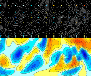
In order to provide a qualitative perspective on the performance of the algorithm, figure 3 shows realizations of the flow from case B1 (see table 2), at both (i) the initial and (ii) the final ($t^+ = T^+ = 50$) times within the assimilation window. At each instant, the field is visualized using (a) the observational data only, (b) the adjoint-variational prediction, and (c) a detailed comparison of the predicted (colour) and true (lines) states. Recall that the observations from benchmark case B1 are at 1/4096 the resolution of the simulation, since the velocity is observed at every eighth point in each spatial dimension and in time. The quality of the reconstruction is evident in figure 3, with the predictions at the initial time capturing the large scales of the flow, but appearing to contain some small-scale, or high-wavenumber, deviations (figure 3ci). At the final time, in contrast, these small-scale deviations have mostly vanished and the reconstruction quality is, qualitatively, improved (figure 3cii).

Figure 3. Instantaneous spanwise velocity $w$ at $z=L_z/2$ visualized using (a) observational data and (b) true fields (lines) and adjoint-variational prediction (colours) at (i) $t=0$ and (ii) $t=T$ ($T^+=50$). (c) Zoom-in views of (b).

The convergence history of the cost function that generated the assimilated initial condition is shown in figure 4(a). The normalization is performed using the cost function associated with advancing the initial guess which was obtained by spline interpolation of the observations and their projection onto the divergence-free space. The monotonic decrease of the cost function is ensured by the accurate evaluation of its gradient using the discrete adjoint. After 100 L-BFGS iterations, the cost function is reduced to $2.8\,\%$ of its initial value.

Figure 4. (a) Convergence history of the cost function, normalized by its initial value. (b) Volume-averaged error (3.1) of the instantaneous velocity field estimated using different strategies: black dashed line, interpolated initial condition (red circle) is projected onto divergence-free space (black cross) and advanced using the Navier–Stokes equations; black solid line, estimated initial condition using data within $t \in [0,T]$ (grey region) is evolved in time; green solid line, estimated state at $t=2T$ using data within $t \in [2T,3T]$ (green region) is evolved in time.

A quantitative assessment of prediction accuracy starts with an evaluation of the root-mean-square (r.m.s.) errors between the predicted and true states,

(3.1)\begin{equation} {\mathcal{E}}_V({\boldsymbol{u}}) = \langle \| \boldsymbol{u} - \boldsymbol{u}_{{true}} \|^2 \rangle_{V}^{1/2}, \end{equation}

where $\langle \,{\cdot }\, \rangle$ denotes averaging, and the subscript indicates the averaging domain, here over the volume $V$; the same convention is adopted throughout the work for errors $\mathcal {E}$ and correlation coefficients $\mathcal {C}$. When errors and correlation coefficients between the predicted and true fields are reported, they are evaluated throughout the domain, and not only at observation locations.

The time dependence of the estimation error is plotted in figure 4(b). At the initial time, the spline interpolation of the observations (red circle), projection onto the solenoidal space (cross) and the adjoint-variational state all have seemingly similar errors – the last being obtained after 100 L-BFGS iterations. A mild reduction in the initial errors is achieved by the projection, and a further modest improvement is achieved by the variational approach, but the initial errors remain approximately $4\,\%$ of the bulk velocity, which is of the same order of magnitude as the r.m.s. fluctuations. An important difference arises, however, when the initial conditions are advanced in time. When the interpolated observations are projected onto the divergence-free field and marched using the Navier–Stokes equations (dashed line), without any data assimilation, the errors amplify as expected due to the chaotic nature of the flow. At long times, after a transient divergence, nonlinear effects become dominant and thus the estimation error saturates. Simply performing spatiotemporal interpolation of the observations would maintain lower errors, similar to the red circle, although that would not be a solution to the governing equations. Now consider the errors when the initial condition is obtained from the adjoint-variational state estimation (solid line). The initial errors in the assimilated field decay with time, and the flow more closely tracks the trajectory of the true field in state space during the observation window (shaded region, $0 \leqslant t \leqslant 4.5$). At $t=T$, the errors are an order of magnitude smaller than those from interpolating and advancing the initial condition or performing spatiotemporal interpolation of observations.

Beyond the observation window, the estimated state again diverges from the truth but remains more accurate than evolving the interpolated initial field during the interval $[T, 3T]$. These results demonstrate the potential of the algorithm to provide a better prediction of the future state $t>T$, when observations are not available. If new data do become available at later times, the estimated state can be adopted as the initial guess, and the same variational procedure can be applied to drive the estimated state towards the true state, again. This idea is demonstrated in figure 4(b): new observation data were provided in the interval $t \in [2T, 3T]$, which is marked by the light grey region. The adjoint-variational algorithm was applied in that new interval, and the predicted state at $t=2T$ now yields a new trajectory that more closely follows the true flow (green line). While this point was noteworthy, the focus of the present effort is on characteristics of the state estimation in the first window $t \in [0, T]$, which are generally applicable to any subsequent interval of new observations.

The r.m.s. estimation error evaluated in the horizontal plane, $\mathcal {E}_{xz} (q)$, are plotted as a function of wall-normal direction in figure 5. The errors in the interpolated initial guess (dashed lines) are proportional to the level of physical fluctuations in the velocity field and, as a result, the errors in the streamwise component are most dominant especially in the near-wall region where $u$-perturbations are most energetic. The estimated initial condition (thin black line) is slightly improved relative to the interpolated state. The key observation is, however, at $t=T$, where all three components of errors in the estimated state are an order of magnitude more accurate than advancing the interpolated state using the forward model. For the streamwise component, the error is less than $0.5\,\%$ of the bulk velocity, or, equivalently, $8\,\%$ of the peak value of r.m.s. streamwise fluctuation. Figure 5(b) also shows the correlation coefficient,

(3.2)\begin{equation} \mathcal{C}_{xz}(q) = \frac{ \langle q\,q_{{true}}\rangle_{xz} } {{\langle q^2 \rangle_{xz}^{1/2}} { \langle q_{{true}}^2 \rangle_{xz}^{1/2}}}. \end{equation}

At $t=T$, the estimated and the true fields are nearly perfectly correlated, which highlights the capacity of the assimilated field to reproduce the true trajectory of the flow in state space.

Figure 5. Wall-normal profiles of (black curves) horizontally averaged errors $\mathcal {E}_{xz} (q)$ and (red curves) correlation coefficient $\mathcal {C}_{xz}(q)$ (3.2) between the estimated and true flow states: (a) streamwise, (b) wall-normal and (c) spanwise components. Lines: black dashed line, spline interpolation of observed velocity field at $t=0$; black and red solid thin lines, adjoint-variational estimation at $t=0$; and black and red solid thick lines, estimation at $t=T$ ($T^+ = 50$).

In order to explain the improvement in accuracy during the observation time horizon, we evaluate the spectra of the estimation error,

(3.3)\begin{equation} \mathcal{E}_y (\hat{\boldsymbol{u}}) = \langle \| \hat{\boldsymbol{u}} - \hat{\boldsymbol{u}}_{{true}} \|^2 \rangle_y^{1/2}, \end{equation}

where $\hat {\boldsymbol {u}}$ is the Fourier transform of $\boldsymbol {u}$ in the streamwise and spanwise directions. The spectra of the errors are reported in figure 6(a) as a function of the horizontal $(k_x, k_z)$ wavenumbers; also shown in figure 6(b) is the spectrum of the true velocity field. Errors appear largest in the low-wavenumber modes, but they should be viewed relative to the high energy content in these modes in figure 6(b). Normalized by the spectral density in the true field (see figure 6c), low wavenumbers are better reconstructed since they are encoded in the sparse observations. A more important observation is the behaviour of the high-wavenumber components of the errors. The estimated initial condition (figure 6ai) has appreciable errors in those wavenumbers (higher than the interpolated state – not shown). However, since most of these modes decay with time (figure 6aii), they have little impact on the estimation quality later within the assimilation time horizon. In addition, due to their rapid decay, these high-wavenumber initial errors do not appreciably affect the value of the cost function, which is integrated over the entire observation window. As a result, they persist in the initial condition during the optimization procedure. An effective strategy to reduce these initial high-wavenumber errors is to incorporate time-dependent weights in the cost function, which amplify the contribution of early observations near $t=0$ (Wang et al. Reference Wang, Wang and Zaki2019a). One should caution, however, that not all the initial high-wavenumber errors are stable and decaying. Small components of that error are unstable and amplify at the Lyapunov rate, and, although they are not perceptible within the present time horizon, they will dominate at longer times.

Figure 6. (a) Fourier spectrum of errors from adjoint-variational estimation, averaged in $y$ and normalized by the bulk velocity, $\log _{10}\mathcal {E}_y (\hat {\boldsymbol {u}})$. (b) Spectrum of the true velocity field averaged in time and wall-normal direction, $\log _{10} \langle \| \hat {\boldsymbol {u}}_{{true}} \|^2 \rangle ^{1/2}_{yt}$. (c) Same as (a) with the errors normalized by $\langle \| \hat {\boldsymbol {u}}_{{true}} \|^2 \rangle ^{1/2}_{yt}$. Panels: (i) $t=0$ and (ii) $t=T$ ($T^+ = 50$). Wavenumbers $(k_x,k_z)$ are normalized by the half channel height.

Consistent with the above integral and spectral measures of the estimation quality, the reconstructed velocity field at $t = T$ is almost identical to the true one (side views in figure 7). An accurate estimation of vortical structures is, however, more challenging since the computation involves velocity gradients. These structures are visualized using the $\lambda _2$ vortex identification criterion (Jeong & Hussain Reference Jeong and Hussain1995) and compared in figure 7 (grey isosurfaces). The prediction of vortical structures is very compelling, in both the near-wall and outer regions. In the former, the vortical tubes are attached to the wall and elongated in the streamwise direction. Farther from the wall, the lifted vortical tubes break down and generate small-scale structures that are mostly captured by the estimated state. In practice, reconstructing the vorticity field from coarse-resolution experimental data is a challenge (Suzuki Reference Suzuki2012). The satisfactory estimation quality in figure 7($b$) demonstrates the potential of our algorithm to augment under-resolved turbulent data from experiments.

Figure 7. Comparison of (a) true and (b) adjoint-variational estimated state at $t=T$ ($T^+ = 50$). Grey isosurfaces: vortical structures visualized using the $\lambda _2\ $ vortex identification criterion with threshold $\lambda _2 = -2$. Side view: contours of spanwise velocity.

3.2. The influence of noise in the observation data

In the previous section, the observation data were free of any noise. In practice, however, experimental measurements invariably contain errors and, as such, may violate the governing equations, lead to statistical errors and severely preclude accurate evaluation of derivatives, especially in turbulent flows where strong velocity gradients are expected (see e.g. Bardet, Peterson & Savaş Reference Bardet, Peterson and Savaş2010). For example, Abrahamson & Lonnes (Reference Abrahamson and Lonnes1995) assessed the ability of conventional circulation and least-squares methods to reproduce the vorticity field from a randomly perturbed DNS velocity field. When $5\,\%$ noise was superposed onto the fully resolved velocity data, the uncertainty in the computed vorticity field reached $40\,\%$, and most of the small-scale structures were absent in the reconstruction.

In order to evaluate the performance of the adjoint-variational algorithm with noisy data, we contaminate the observed velocities by Gaussian random noise with standard deviation that is proportional to the local velocity component (2.5a,b). The spatiotemporal resolution of the data and the estimation window $T^+ = 50$ remain the same as in the benchmark case. We consider three levels of noise: $\sigma = \{0, 5, 10\}\,\%$, which correspond to cases B1, N1 and N2 in table 2. The first guess of the initial condition is interpolation of the noisy data at $t=0$.

After 100 L-BFGS iterations, the cost function is decreased to $\{2.8 , 27 , 45\}\,\%$ for the three levels of contamination. Since the cost function is defined as the difference between the estimated and contaminated data, and the latter do not satisfy the Navier–Stokes equations, the cost function cannot decrease to zero. The r.m.s. error of the estimated state relative to the true, uncontaminated flow field was evaluated and shows a similar decay from the initial to the final time as in the benchmark case without noise. Therefore, only the results at $t=T$ are examined here (figure 8). The estimation error increases with the noise level (from light grey to black lines), but remains within $2\,\%$ of the bulk velocity. Note that, due to the mean flow, the observation noise in the streamwise direction can exceed $\sigma$ times the bulk velocity, which means that the estimation accuracy of the streamwise velocity actually exceeds the precision of observation data. Comparatively, the estimation errors of the wall-normal and spanwise velocity components are bounded by the observation noise, which is approximately $\sigma$ times the r.m.s. turbulence fluctuations. Overall, even with the highest noise level ($\sigma = 10\,\%$), the correlation coefficient (3.2) between the estimated and true state is close to unity at all the $y$ locations, as shown by the red lines in figure 8(b).

Figure 8. Effect of observation noise level on (grey to black, $\sigma = \{0, 5, 10\}\,\%$) estimation error $\mathcal {E}_{xz}(q)$ and (red, $\sigma = 10\,\%$) correlation coefficient $\mathcal {C}_{xz}(q)$ at $t=T$ ($T^+ = 50$): (a) streamwise, (b) wall-normal and (c) spanwise components.

The reconstructed vortical structures are visualized in figure 9. Although some of the small-scale structures are not captured, most of the reconstructed wall-attached and detached vortical structures remain nearly identical to the true flow, and the estimation quality is almost independent of the noise level. A quantitative assessment of the quality of the vorticity field is provided in figure 10. When noisy observations are interpolated and vorticity is evaluated, the error (dashed lines) in the near-wall region reaches 10–40 % of the mean vorticity at the wall. The error of the vorticity field from adjoint-variational estimation (black solid lines) is within $4\,\%$ of the wall vorticity, and the estimation accuracy is robust against observation noise. These results demonstrate the superiority of the adjoint-variational approach for evaluating velocity gradients and its robustness to observation noise.

Figure 9. Comparison of (a) true vortical structures and (b,c) the adjoint-variational reconstruction when $\sigma = \{5, 10\}\,\%$ at $t=T$ ($T^+ = 50$) within the bottom half channel, visualized using the $\lambda _2$ vortex identification criterion with threshold $\lambda _2 = -2$.

Figure 10. Horizontally averaged error $\mathcal {E}_{xz}(q)$ of vorticity field at $t=T$ ($T^+ = 50$), estimated by (black dashed line) interpolating noisy velocity data and (black solid line) adjoint-variational approach (grey to black, noise level $\sigma = \{0, 5, 10\}\,\%$): (a) streamwise, (b) wall-normal and (c) spanwise components. The error is normalized by mean vorticity $\langle \textrm {d}u / {\textrm {d} y}\rangle$ at the wall.

3.3. The effect of spatial and temporal data resolution

Although the results thus far have demonstrated the accuracy of the flow reconstructions, it is expected that the estimation quality depends on the spatiotemporal resolution of the observations. And it is also of interest to query the lowest resolution requirement for accurate estimation. In homogeneous isotropic turbulence, it has been reported that reconstruction of the full field is successful only if the resolution of spatial observations satisfies $\varDelta _m < 15 \eta$ (Li et al. Reference Li, Zhang, Dong and Abdullah2020), where $\eta$ is the Kolmogorov length scale. An equivalent criterion has not, however, been proposed for anisotropic, wall-bounded turbulence, where the effects of mean shear, advection and the no-slip boundary may alter the resolution requirements of the observations. Hereafter, we revert to adopting noise-free data and focus on the influence of spatiotemporal resolution of observations on the accuracy of state estimation within the time horizon $T^+ = 50$.

We first consider the impact of spanwise spacing of observations that are fully resolved in the $x$–$y$ plane (cases RZ1–RZ4 in table 2). With the most coarse observations ($\Delta z_m^+ = 112$, case RZ4), the estimated state is visualized in figure 11 and compared to the true one. At the observation locations ($z = z_m$), velocity data are reproduced by the algorithm. At the midpoint between observation planes ($z = z_m + 0.5 \Delta z_m$), however, the estimation accuracy is notably compromised.

Figure 11. The (lines) true streamwise fluctuation $u - \langle u \rangle$ at $t=T$ ($T^+ = 50$) and (colours) estimation with data resolution $\Delta z_m^+ = 112$ (case RZ4 in table 2). The fields are visualized at (a) an observation plane, $z = z_m$, and (b) the midpoint between two observation planes, $z = z_m + 0.5 \Delta z_m$.

Since our interest is in the distribution of errors between observation planes, the estimation error is phase-averaged in the span in addition to averaging in the streamwise direction, and is denoted $\mathcal {E}_{xz_m}(q)$. The results for cases RZ1–RZ4 are shown in figure 12. Only the error for the $u$ component is plotted, and the results for the $v$ and $w$ components are similar. With the most poorly resolved data (figure 12a), the estimation error increases by an order of magnitude from the observation planes to the midpoint between them. The error in the near-wall region is of the same order of magnitude as the local turbulence fluctuations, which is significantly higher than the error at the channel centre. As better-resolved observations are adopted (figure 12b–d), the inhomogeneity of the error distribution in the spanwise direction becomes weaker.

Figure 12. Streamwise- and phase-averaged estimation error $\mathcal {E}_{xz_m}(u)$ between two $x$–$y$ observation planes at $t=T$ ($T^+ = 50$), normalized by the true local r.m.s. fluctuations $u^{\prime }_{rms}$: (a–d) $\Delta z^+_m = \{112,56,28,14\}$, respectively.

The effect of spanwise data resolution can be explained by examining the spanwise two-point correlations $\mathcal {R}_u(\Delta z)$ in figure 13(ai). Since the dominant structures in the wall layer are streaks and streamwise vortices that are narrow in the span, the two-point correlation decays faster at locations closer to the wall. As a result, the domain of dependence of the observation planes shrinks from channel centre to the wall, which explains the high estimation error in the wall layer. Figure 13(aii) shows the reconstruction quality at $t=T$ in terms of the correlation coefficient between the true and estimated states from the least-resolved data ($\Delta z_m^+ = 112$). The profiles are qualitatively similar to the two-point correlations within $\Delta z^+ < 20$. However, while the turbulent structures decorrelate at larger distances, the accuracy of the reconstruction remains relatively higher, and $\mathcal {C}_{xz_m}(u^{\prime })$ returns to approximately unity as we approach the next observation plane at $z^+ - z^+_m = 112$.

Figure 13. (ai) Two-point correlations $\mathcal {R}_u$ of the true streamwise fluctuation as a function of spanwise separation; and (aii) correlation coefficient $\mathcal {C}_{xz_m}(u^{\prime })$ between estimated (case RZ4, $\Delta z_m^+ = 112$) and true streamwise fluctuations at $t = T$ ($T^+ = 50$) as a function of distance from observation planes. Grey to black correspond to $y^+ = \{17, 51, 180\}$. The horizontal dotted line marks zero correlation. (b) Wall-normal profiles of (red dashed line) Kolmogorov length scale and Taylor microscales based on (black solid thin line) correlation coefficient $\mathcal {C}_{xz_m}(u^{\prime })$ and (black dashed line) spanwise two-point correlations. (c) Streamwise Taylor microscales based on two-point correlations of (black dashed line) $u$, (blue dashed line) $v$ and (green dashed line) $w$ components.

Similar to the notion of the Taylor microscale,

(3.4)\begin{equation} \varLambda_{z,u} = \left(\left.-\frac{1}{2}\frac{\textrm{d}^2 \mathcal{R}_u}{\textrm{d} (\Delta z)^2} \right|_{\Delta z = 0} \right)^{{-}1/2}, \end{equation}

we introduce a length scale for the domain of dependence of one observation plane by replacing $\mathcal {R}_u$ in (3.4) by the correlation coefficient $\mathcal {C}_{xz_m}(u^{\prime })$. The resulting length scale, which we denote $\varLambda _{Cz}$, is representative of the domain of accurate estimation. Both $\varLambda _{z,u}$ and $\varLambda _{Cz}$ are plotted in figure 13(b), and have similar values across the height of the channel: the spanwise size of the domain of dependence of observations is similar in the Taylor microscale. Therefore, the criterion

(3.5)\begin{equation} \Delta z_m \lesssim 2\varLambda_{z,u} \end{equation}

must be satisfied to guarantee an accurate estimation of the local $u$ field. Similar criteria can be adopted for accurate estimation of the $v$ and $w$ components using the Taylor microscales $\varLambda _{z,v}$ and $\varLambda _{z,w}$, respectively. Since those length scales are commensurate with $\varLambda _{z,u}$, the condition (3.5) suffices. Using (3.5), we can also interpret the estimation results with different spanwise data resolutions (figure 12). When $\Delta z^+_m = 56$ (figure 12b), the criterion (3.5) is satisfied for the bulk of the channel ($2\varLambda ^+_{z,u} \approx 80$, cf. figure 13b) and starts to be violated for $y^+ < 70$. As such, while figure 12(b) reports high prediction accuracy in the bulk ($\mathcal {C}_{xz_m}(u') = 0.97$), errors increase in that near-wall region ($\mathcal {C}_{xz_m}(u') = 0.83$) and become inhomogeneous in the span. When $\Delta z^+_m = 28 < \min _y 2\varLambda _{z,u}^+$ (figure 12c), every point in the flow is covered by the domain of dependence of observations, so the estimation quality becomes more accurate and uniform at all the $y$ locations ($\mathcal {C}_{xz_m}(u') = 0.99$).

We compare the criterion (3.5) to that for homogeneous isotropic turbulence (Yoshida et al. Reference Yoshida, Yamaguchi and Kaneda2005; Lalescu et al. Reference Lalescu, Meneveau and Eyink2013; Li et al. Reference Li, Zhang, Dong and Abdullah2020) that $\varDelta _m \lesssim 15 \eta$. The Kolmogorov scale in our case is $\eta \equiv (Re^3 \mathcal {D})^{-1/4}$, where $\mathcal {D} = (2/Re) \langle s'_{ij} s'_{ij}\rangle$ is the viscous rate of dissipation and $s'_{ij} = (\partial _i u_j^{\prime } + \partial _j u_i^{\prime })/2$ is the fluctuating strain-rate tensor. The criterion $15 \eta$ is plotted as the red dashed line in figure 13(b). Since the average dissipation is affected by the streamwise-elongated structures in the channel, $\eta$ is larger than the spanwise size of the smallest eddies. Nonetheless, the trend is similar to the Taylor microscale condition provided above. Physically, both criteria demonstrate that the critical data resolution for accurate estimation of the entire flow is within the transition zone between the inertial and viscous dissipation ranges.

Next, we consider fully resolved observations in the cross-flow $y$–$z$ planes, and under-resolved in the streamwise direction (cases RX1–RX4 in table 2). Before examining the state estimation results, we report the Taylor microscales $\varLambda _{x,i}$ ($i=u,v,w$) in figure 13(c), which is computed from the streamwise two-point correlations. Owing to the near-wall elongated streaky structures, $\varLambda _{x,u}$ is largest among all three components, peaks near the wall and decays towards the channel centre. We therefore expect that the estimation, particularly of the $u$ component, should be most accurate in the inner layer relative to the accuracy in the outer flow.

The r.m.s. estimation error is plotted in figure 14, where $\mathcal {E}_{x_mz}(u)$ is averaged in the span and phase-averaged in the streamwise direction, and also normalized by the r.m.s. fluctuations. Overall, the estimation error decreases as better-resolved data are included (figure 14a–d). For each observation resolution, the estimation quality deteriorates from the wall to the channel centre, as expected. Two notable differences from the effect of spanwise resolution are observed: (i) the estimation error is not symmetric with respect to the midpoint between observation planes, especially in figure 14(a,b); and (ii) although the separation of observation planes in figure 14(a) is larger than $2\varLambda ^+_{x,u}\ (\approx 118)$ in the bulk (cf. figure 13c), the estimation error does not increase appreciably between streamwise observation locations and remains within approximately $10\,\%$ of the local r.m.s. fluctuations ($\mathcal {C}_{x_mz}(u^{\prime }) \geqslant 0.95$ while $\mathcal {R}_{u}(\Delta x^+=96) \approx 0.6$). Both points are caused by the mean advection in the streamwise direction. Conceptually, every instant when data are recorded in the cross-flow $y$–$z$ plane corresponds to an accurately estimated ‘layer’ in the spatiotemporal evolution of the flow, propagating by the advection velocity $U_a$. The thickness of such layers is approximately the Taylor microscale $\varLambda _{x,u}$, and the distance between two adjacent ones is approximately $U_a \Delta t_m$. Since the observation data are temporally well resolved, $U_a \Delta t_m \ll 2\varLambda _{x,u}$, the accurately estimated layers overlap with one another and lead to commensurate accuracy between observation locations. An example that further highlights this conceptual interpretation is considered next, where the temporal sampling rate is sufficiently low ($U_a \Delta t_m > 2\varLambda _{x,u}$) in order to distinguish the accurately predicted layers associated with different ($x_m,t_m$).

Figure 14. Spanwise- and phase-averaged estimation error $\mathcal {E}_{x_m z}(u)$ between two $y$–$z$ observation planes at $t=T$ ($T^+ = 50$), normalized by the true local r.m.s. fluctuations $u^{\prime }_{rms}$: (a–d) $\Delta x^+_m = \{192,96,48,24\}$, respectively.

Consider the same coarse spatial resolution from case RX4 ($\Delta x^+_m = 192$), and we now adopt a long time between observations, $\Delta t^+_m = 7.4$. This case is denoted RT4, and a temporal evolution of the estimation error from $t = 0$ to $t = \Delta t_m$ is shown in figure 15. Three layers of small errors are observed: $A$ originates at the observation station at $t=0$ and advects downstream; $B$ emerges between observation locations and times, such that the field accurately reproduces measurements at a downstream observation point at a subsequent measurement time $t = \Delta t_m$; and $B^{\prime }$ is similar to $B$ but reaches the observation station at $t = 2\Delta t_m$. Once $A$ leaves the observation plane, the error increases, at least initially, due to the chaotic nature of turbulence and the absence of a nearby observation station to correct the field – behaviour later in time is discussed below. By comparison, the error in $B$ decays with time as it approaches the observation location at time $t=\Delta t_m$.

Figure 15. Spanwise- and phase-averaged estimation error $\mathcal {E}_{x_mz}(u)$ within the first observation time interval ($\Delta t^+_m = 7.4$, $T^+ = 50$, case RT4): (a–e) $t = \{0.00, 0.25, 0.50, 0.75, 1.00\}\Delta t_m$, respectively. Blue regions: $A$, regions where error is low at $(x,t) = (x_m,0)$ and advected downstream; $B$, emergent region of small error that later coincides with observation plane $(x,t)=(x_m,\Delta t_m)$; and similarly $B^{\prime }$ coincides with $(x,t)=(x_m,2\Delta t_m)$.

A detailed space–time representation of the estimation error at the channel centre is shown in figure 16. All the regions of small errors (blue) belong to one of the three classes described above, and can be associated with at least one observation station (black plus signs). The pattern of the errors is repeated, anchored at $(\Delta x_m, \Delta t_m)$ and inclined according to the advection speed. Since $3U_a \Delta t_m \approx 2 \Delta x_m$, regions $A_i$ that originate from $(x,t) = (x_m, 0)$ will reach another observation station at $(x,t) = (x_m + 2 \Delta x_m, 3 \Delta t_m)$; the errors in that region thus initially increase moving away from $(x_m,0)$ and reduce as that later observation point is approached. For a general spatiotemporal resolution of observations, regions $A_i$ may not coincide with another observation position and time, and hence the errors would not undergo the later decay. From figure 16, it is evident that an accurate estimation of the entire flow state can be achieved by refining either the spatial or temporal data resolution such that the low-error regions overlap. This view is demonstrated in figure 17(a–d) where the panels correspond to increasing temporal resolution (cases RT4–RT1, respectively, in table 2). When the true state is observed sufficiently frequently, the estimation error in the bulk region approaches homogeneity in the streamwise direction (figure 17c,d). Specifically, accurate reconstruction is achieved when the distance between the thin layers that sample observation points is within the domain of dependence of observations,

(3.6)\begin{equation} U_a \Delta t_m \lesssim 2\varLambda_{x,u}. \end{equation}

Recalling that $\varLambda _{x,v} \approx \varLambda _{x,w} < \varLambda _{x,u}$ (cf. figure 13c), the equivalent criterion for accurate estimation of $v$ and $w$ is more restrictive. When the observations only satisfy the bound for $u$, the reconstruction is less accurate for the other two velocity components (e.g. $\mathcal {C}_{x_mz}(u',v,w) = \{0.95, 0.86, 0.79\}$ when $\Delta x^+_m = 192$ and $\Delta t^+_m = 7.4$).

Figure 16. Space–time evolution of the spanwise-averaged estimation error $\mathcal {E}_z(u)$ at the channel centre. Black plus sign, observation location and time; $A_i, B_i, B_i^{\prime }$, same as $A, B, B^{\prime }$ in figure 15; and the subscript denotes the $i\textrm {th}$ interval between streamwise observations.

Figure 17. Spanwise- and phase-averaged estimation error $\mathcal {E}_{x_mz}(u)$ at $t=T$ ($T^+ = 50$) with different observation time interval: (a–d) $\Delta t^+_m = \{7.4, 3.7, 1.8, 0.9\}$, respectively.

In summary, to guarantee an accurate estimation of local velocity component $i$, the streamwise and temporal data resolution must satisfy either one of two conditions:

(3.7)\begin{equation} \textrm{(i)}\ \Delta x_m \lesssim 2\varLambda_{x,i}\ \textrm{and}\ \Delta t_m \lesssim \tau_{\sigma} \quad \textrm{or} \quad \textrm{(ii)}\ \Delta t_m \lesssim 2\varLambda_{x,i}/U_a\ \textrm{and}\ \Delta x_m \lesssim U_b\tau_{\sigma} . \end{equation}

The first condition is similar to that for the spanwise data resolution, namely that the Taylor microscale must be resolved by observations. Note that it is supplemented by a statement regarding the observation time, which must be smaller than the Lyapunov time scale $\tau _\sigma$ because even a near-perfect estimate of the flow state will diverge from the true solution over that period unless additional data are available for assimilation. The second condition is a reinterpretation that accounts for mean advection: should the temporal resolution resolve the advected Taylor scale, the only requirement for spatial resolution becomes a condition based on the travel distance within the Lyapunov time. These two conditions are plotted in figure 18. We performed additional tests with $\Delta x_m^+ = 48$ and $\Delta t^+_m = \{0.45, 0.90, 1.80, 3.70, 7.40\}$. When the correlation coefficient between the true and estimated states was higher than 90 %, the outcome was deemed successful; these cases are marked by circles. Inaccurate, or unsuccessful, reconstructions are marked by crosses. The outcomes of all the cases agree with the above two conditions.

Figure 18. Criteria for streamwise and temporal data resolutions: (black line) $\Delta t_m = \tau _{\sigma }$ and $\Delta x_m = \min _{y,i} (2\varLambda _{x,i})$; (blue line) $\Delta t_m = \min _{y,i} (2\varLambda _{x,i}) / U_b$ and $\Delta x_m = U_b \tau _{\sigma }$; (empty circles) successful estimation with correlation coefficient higher than 0.9; (crosses) unsuccessful estimation.

3.4. Estimation without wall-layer data

In all the above cases, observations were distributed throughout the wall-normal extent of the channel, spanning both the inner and outer layers. In reality, however, experimental observations become progressively more difficult to obtain near the wall (Hutchins, Hambleton & Marusic Reference Hutchins, Hambleton and Marusic2005; Smits, McKeon & Marusic Reference Smits, McKeon and Marusic2011). And since most of the turbulence kinetic energy is produced near the wall (peak production at $y^+ \approx 12$) and transported into the bulk region, lack of observation in this region may severely compromise the estimation of the full state. We therefore explore the accuracy of reconstructing the flow within the inner region when observations are only available in the outer layer and directly on the wall. Previous efforts for this configuration are limited and have generally focused on use of linear models (Baars, Hutchins & Marusic Reference Baars, Hutchins and Marusic2016; Illingworth, Monty & Marusic Reference Illingworth, Monty and Marusic2018). The present test case is the first attempt to perform a reconstruction based on the full nonlinear Navier–Stokes equations.

Specifically, we consider two types of observations: (i) subsampled velocity data available in the outer layer, $y^+>30$, with the same spatial and temporal resolution as the benchmark case; (ii) shear stresses $\boldsymbol {\tau } = (\tau _{xy}, \tau _{zy})$ on both channel walls with the same resolution as velocity data. The observation time horizon is the same as the benchmark case, $T^+ = 50$. These observations are weighted in the cost function,

(3.8)\begin{equation} J(\boldsymbol{u}^0) = \tfrac{1}{2} \sum_{n=0}^N [ \| \boldsymbol{u}^n_m - \mathcal{M}_u(\boldsymbol{u}^n) \|^2 + \left(\beta Re / Re_\tau \right)^2 \| \boldsymbol{\tau}^n_m - \mathcal{M}_{\tau}(\boldsymbol{u}^n) \|^2_w ], \end{equation}

where $\| \cdot \|_w$ represents integration over top and bottom walls and the weight $\beta = 1/5$. The choice of weighting parameter $\beta$ may be motivated by different objectives, such as balancing the two contributions in the cost function or their gradients or minimizing the condition number of the Hessian of $\mathcal {J}$. Here we adopt $\beta =1/5$ such that the stress term is commensurate with the velocity at the first fluid grid point that was observed in our benchmark case. The estimated state is compared with the benchmark case to highlight the impact of missing observations in the wall layer.

The predicted statistics without wall-layer observations, evaluated at $t=T$, are plotted in figure 19 and are compared with the true statistics. The quantities shown are horizontally averaged; the corresponding turbulence kinetic energy equation is

(3.9)\begin{equation} \frac{\partial E}{\partial t} = \underbrace{-\langle u'_i u'_j \rangle \frac{\partial \langle u_i\rangle }{\partial x_j}}_{\mathcal{P}} -\frac{\partial }{\partial x_j} \left(\frac{1}{2}\langle u'_i u'_i u_j\rangle + \langle u'_j p\rangle - \frac{2}{Re} \langle u'_i s'_{ij} \rangle \right) - \underbrace{\frac{2}{Re} \langle s'_{ij} s'_{ij}\rangle }_{\mathcal{D}}. \end{equation}

The estimated profiles are accurate, even within the viscous sublayer and buffer layer, which are void of observations and where production and dissipation predominate. Although the interpolated initial condition also converges to the true statistics after a long time ($t \approx 4T$), our estimated state reaches the statistically stationary state faster ($t \approx 1.5T$), especially for dissipation. The errors in the estimated instantaneous velocity fields are shown in figure 20. Compared with the benchmark case (grey lines), the estimation quality in the outer layer is almost unaffected when the wall-layer data are removed. In the near-wall region, however, the estimation error reaches a maximum and exceeds twice the error in the benchmark case. The streamwise component is the most poorly reconstructed. Without data in the wall layer, the data assimilation algorithm starts with an interpolated velocity field as a first guess, which underestimates the mean flow near the wall; the final prediction of the algorithm retains a similar deficit in the mean, and hence the estimation error is largest in the streamwise component (black lines in figure 20). At $t=T$, the highest estimation error is approximately $4\,\%$ of the bulk velocity, which is smaller than the $16\,\%$ local r.m.s. streamwise turbulence fluctuations. In addition, the correlation coefficient between the true and estimated states at $t=T$ is above 0.8 for all three components of the velocity field.

Figure 19. Comparison of the instantaneous ($t=T$, $T^+ = 50$), horizontally averaged flow statistics for the (grey circles) true and (black lines) estimated fields, without wall-layer observation data: (a) r.m.s. fluctuations; and (b) turbulence kinetic energy (TKE) production and dissipation. Dashed lines, $y^+ = 30$.

Figure 20. Comparison of the estimation errors $\mathcal {E}_{xz}(q)$ (grey) with and (black) without wall-layer observation data: (a) streamwise, (b) wall-normal and (c) spanwise components at (thin) $t=0$ and (thick) $t=T$ ($T^+ = 50$). Red: correlation coefficient $\mathcal {C}_{xz}(q)$ between the true and estimated states without wall-layer observation data at $t=T$. Dashed line, $y^+ = 30$.

The wall layer is host to coherent structures, such as streaks and streamwise vortices, that play an important role in the dynamics of the near-wall turbulence cycle (Hamilton, Kim & Waleffe Reference Hamilton, Kim and Waleffe1995) and in flow control. For example, the streak spacing must be resolved by a controller in order to effectively relaminarize turbulent channel flow (Sharma et al. Reference Sharma, Morrison, McKeon, Limebeer, Koberg and Sherwin2011). Accurate prediction of these structures is therefore important. The error of our estimation at different length scales is reported in figure 21. The most accurately reconstructed structures are long in the streamwise direction ($\lambda _x \approx O(L_x)$) and large waves in the span ($\lambda ^+_z \in (10^2,10^3)$), which are typical features of near-wall streaks and streamwise vortices (Jiménez Reference Jiménez2018). The estimation error of these structures is mildly affected by removing the wall-layer data, due to their coherence across wall-normal locations, which facilitates the estimation even without near-wall observations. In contrast, reconstruction of small-scale near-wall structures is more sensitive to the lack of observations in that region, which is symptomatic of the weaker sensitivity of the outer flow to these structures.

Figure 21. One-dimensional Fourier spectra of estimation error at $y^+ = 15$, averaged within $t\in [0.5, 1.5]T$ and normalized by the amplitude of the corresponding Fourier modes: (a) streamwise spectrum averaged in the span; and (b) spanwise spectrum averaged in the streamwise direction. Estimation (grey line) with and (black line) without wall-layer observation data.

Despite the overall increase of estimation errors when wall-layer data are not available, the instantaneous visualization of the coherent structures can still be compelling. Figure 22 shows a visualization of the predicted instantaneous streamwise fluctuation velocities for two predictions: without and with observations in the wall layer. The estimated streaky structures without wall-layer observations (figure 22ai) are irregularly spaced in the spanwise direction and meander downstream, as expected from a realistic channel flow. The zoomed-in view (figure 22aii) also includes the true state (line contours), which confirms that the state estimation is predictive: the true streaks are reproduced. The estimation accuracy is in fact comparable to the case when observations are available in the wall layer (figure 22b). The successful estimation of the missing wall layer is directly tied to the sensitivity of the observations in the outer flow and at the walls to the state in this region at the initial time. In other words, accurate reconstruction of the inner layer at the initial time is indispensable to match future observations far from the wall, and is manifest in figure 22 by the accurate prediction of the flow state at the final time.

Figure 22. Streamwise fluctuations at $y^+ = 15$ and $t=T$ ($T^+ = 50$), calculated by subtracting the true mean velocity: estimations (a) without and (b) with wall-layer data. Lines: true fluctuation fields.

3.5. Estimation from wall observations

In practice, control of wall-bounded turbulence may rely on sensing and actuation at the wall, and effective strategies are often predicated on decoding the wall signature of outer turbulence structures. It has been demonstrated both mathematically (Lighthill Reference Lighthill1963; Constantin & Iyer Reference Constantin and Iyer2011) and numerically (Eyink, Gupta & Zaki Reference Eyink, Gupta and Zaki2020a,Reference Eyink, Gupta and Zakib) that all the interior vorticity is generated at the wall. The converse problem, specifically to what extent the initial flow state can be predicted from wall observations, has not been addressed as comprehensively. Previous efforts at $Re_{\tau }=100$, and using a variety of approaches, yielded an estimated state that is nearly uncorrelated with the true flow beyond the buffer layer (Bewley & Protas Reference Bewley and Protas2004; Suzuki & Hasegawa Reference Suzuki and Hasegawa2017; Liu & Hasegawa Reference Liu and Hasegawa2020). The modest Reynolds number in those studies does not support the presence of large-scale outer structures that appreciably influence the wall stress fluctuations (Abe, Kawamura & Choi Reference Abe, Kawamura and Choi2004). LSE has been applied at higher $Re_{\tau }$ to reconstruct large-scale structures in the log layer from wall observations (Encinar & Jiménez Reference Encinar and Jiménez2019). However, the predicted state from LSE does not satisfy the Navier–Stokes equations. Here we focus on adjoint-variational state estimation, specifically on the accuracy of the predicted state and the domain of dependence of wall observations. The dependence on Reynolds number will be examined for $Re_{\tau } = \{100, 180, 392, 590\}$. The computational domain and grid resolution are summarized in table 3. Note that a smaller domain size is adopted for the $Re_{\tau } = \{392, 590\}$ cases due to the limited computational resources.

Table 3. Computational set-up of cases with wall observations (§ 3.5).

The observations are fully resolved shear stresses $\boldsymbol {\tau } = (\tau _{xy}, \tau _{yz})$ and pressure $p$ at both walls, similar to those adopted by Bewley & Protas (Reference Bewley and Protas2004) at the lower Reynolds number. The corresponding cost function is defined as

(3.10)\begin{equation} J(\boldsymbol{u}^0) = \tfrac{1}{2} \sum_{n=0}^N [ \| \boldsymbol{\tau}^n_m - \mathcal{M}_{\tau}(\boldsymbol{u}^n) \|^2_w + \| p^n_m - p^n \|^2_w ]. \end{equation}

For all the different $Re$ cases, the estimation window is the same in viscous units, $T^+ = 50$, which is long enough for perturbation in the bulk region to affect wall signals. The first guess of the initial condition is an LSE of the flow using observations at $t=0$. The stochastic estimator was constructed with a completely independent time series. All the estimated flows are obtained after 100 L-BFGS iterations of the state estimation 4DVar algorithm.

The correlation coefficients of the estimated and true fluctuating velocities at $t=T$ are shown in figure 23. The $Re_{\tau } = 100$ results are comparable to those in figure 6(a) of Bewley & Protas (Reference Bewley and Protas2004) at the same Reynolds number. As $Re_{\tau }$ is increased, the correlation near the wall slightly deteriorates but remains sufficiently high to provide confidence in predictions. Precisely, for all Reynolds numbers, $C_{xz} > 0.8$ when $y^+ < 15$. The correlations start to decay beyond the buffer layer, and those for $v$ and $w$ (figure 23b,c) do so nearly monotonically and with a similar slope for all $Re_\tau$. This trend highlights the challenge of interpreting turbulent flows from wall observations: the accurately predicted near-wall layer is a diminishingly smaller physical region as the Reynolds number is increased. A noteworthy exception is recorded in the correlation coefficients of the streamwise velocity (figure 23a) at $Re_{\tau }=\{392,590\}$: the initial decay outside the buffer layer is followed by a plateau within ($30 < y^+, y < 0.3$) where the reconstruction remains marginally accurate because the large-scale structures in that region superimpose a footprint on wall signals (Abe et al. Reference Abe, Kawamura and Choi2004; Mathis, Hutchins & Marusic Reference Mathis, Hutchins and Marusic2009).

Figure 23. Correlation coefficient $\mathcal {C}_{xz}(q)$ (3.2) between the true and estimated fluctuation fields at $t=T$ ($T^+=50$), evaluated relative to the true mean flow: (a) streamwise, (b) wall-normal and (c) spanwise components. Grey to black: $Re_{\tau }=\{100,180,392,590$}, respectively.

The history of the correlation coefficient $C_{xz}(u')$ at the highest Reynolds number $Re_{\tau }=590$ is shown in figure 24. The adjoint-variational approach yields an evolution of the near-wall flow that is strongly correlated with the true state throughout the observation horizon. It also sustains the plateau in $C_{xz}(u')$ in the outer region that was observed at the final time in figure 23, and which is related to the estimation of the outer large-scale motions. This relation is evident in visualizations of the perturbation fields, e.g. the instantaneous views in figure 25 at $t=T$. In the outer layer, the estimated field matches the mean flow and large-scale motions, while the small-scale fluctuations in the bulk and vortices that are detached from the wall are not captured. These results indicate that the wall signature at these Reynolds numbers is not sensitive to the wall-detached motions in the initial condition – a demonstration of the inherent difficulty of turbulence reconstruction from wall observations.

Figure 24. Time dependence of the horizontally averaged correlation coefficient $\mathcal {C}_{xz}(u^{\prime })$ between true state and adjoint-variational estimation at $Re_{\tau }=590$.

Figure 25. Comparison of (a) true streamwise fluctuation and (b) estimation using wall observations at $t=T$ ($T^+ = 50$), $Re_{\tau }=590$.

In light of the importance of the near-wall turbulence regeneration cycle, we turn to the detail of the true and estimated states in that region. The near-wall streaks (bottom $x$–$z$ planes in figure 25) are accurately reconstructed, and many of the vortical structures (grey isosurfaces in figure 26) are reproduced in the estimated field. Sheng, Malkiel & Katz (Reference Sheng, Malkiel and Katz2009) reported that violent near-wall ejections and sweeps contribute appreciably to the local turbulence energy. Examples of both events are shown in panels (i) and (ii) in figure 26: the true vortex lines above the stress local extrema are closely followed by the estimation, which demonstrates that the extreme events in the buffer layer are encoded in the wall signatures.

Figure 26. (a) True and (b) estimated vortical structures at $t=T$ ($T^+ = 50$) within $y^+ \in [0, 30]$ ($Re_{\tau }=590$), visualized using the $\lambda _2\ $ vortex identification criterion with threshold $\lambda _2 = -15$. Panels (i) and (ii) show (dashed grey) true and (black solid line) estimated vortex lines associated with extreme events: (i) sweep, $(x_s, z_s) = (3.0,0.9)$, vortex lines initiated at $y^+ = 7.6$; (ii) ejection, $(x_e, z_e) = (1.3,2.8)$, vortex lines initiated at $y^+ = 2.3$.

The accuracy of the estimated state can be viewed against the backdrop of the near-wall ‘autonomous cycle’ (Jiménez & Pinelli Reference Jiménez and Pinelli1999; Jiménez & Moser Reference Jiménez and Moser2007). By artificially removing the outer flow in DNS, Jiménez & Pinelli (Reference Jiménez and Pinelli1999) demonstrated that the near-wall dynamics, especially the regeneration cycle of streaks and vortices, is self-sustained. And, as observed in experiments, ‘ejection’ and ‘sweep’ events in that cycle have a wall signature in the form of minima and maxima of the wall shear stress (Sheng et al. Reference Sheng, Malkiel and Katz2009). Here we demonstrate that the wall stress is in fact encoded with the entire dynamics of the regeneration cycle, and our state estimation algorithm decodes these observations to discover the entire flow within the wall layer. The algorithm can also reconstruct the outer large-scale motions when their footprint is encoded in the wall measurements.