2.1 Governing equations and base flow

We consider convective flow in a homogeneous and unbounded three-dimensional porous medium. The flow $\boldsymbol{u}$ is incompressible and satisfies Darcy’s law. The density $\unicode[STIX]{x1D70C}$ of the fluid is linearly related to the temperature $T$ , which is assumed to be locally equilibrated between the solid and fluid phases of the medium and satisfies an advection–diffusion transport equation. These equations are given by

(2.1a,b ) $$\begin{eqnarray}\unicode[STIX]{x1D735}\boldsymbol{\cdot }\boldsymbol{u}=0,\quad \boldsymbol{u}=-\frac{K}{\unicode[STIX]{x1D707}}[\unicode[STIX]{x1D735}p+\unicode[STIX]{x1D70C}g\hat{\boldsymbol{z}}],\end{eqnarray}$$

(2.2a,b ) $$\begin{eqnarray}\unicode[STIX]{x1D70C}=\unicode[STIX]{x1D70C}_{0}(1-bT),\quad \overline{\unicode[STIX]{x1D719}}\frac{\unicode[STIX]{x2202}T}{\unicode[STIX]{x2202}t}+\boldsymbol{u}\boldsymbol{\cdot }\unicode[STIX]{x1D735}T=D\unicode[STIX]{x1D6FB}^{2}T,\end{eqnarray}$$

where $K$ is the permeability of the medium, $\unicode[STIX]{x1D707}$ is the viscosity of the fluid, $p$ is the pressure, $g$ is the gravitational acceleration, $\hat{\boldsymbol{z}}$ is the unit upwards vertical direction, $\unicode[STIX]{x1D70C}_{0}$ is a reference density, $b$ is the coefficient of thermal expansion and $D$ is the average thermal diffusivity, all of which are assumed to be constant. The weighted mass fraction $\overline{\unicode[STIX]{x1D719}}=[\unicode[STIX]{x1D719}+(1-\unicode[STIX]{x1D719})(\unicode[STIX]{x1D70C}_{s}c_{s}/\unicode[STIX]{x1D70C}_{l}c_{l})]$ is defined in terms of the porosity $\unicode[STIX]{x1D719}$ and the specific heats and densities of the solid and liquid phases, $c_{s}$ , $c_{l}$ , $\unicode[STIX]{x1D70C}_{s}$ and $\unicode[STIX]{x1D70C}_{l}$ respectively, and is also assumed to be constant.

Since the velocity field $\boldsymbol{u}=(u,v,w)$ has vanishing vertical vorticity and divergence, it can be written in terms of a scalar velocity-potential function $\unicode[STIX]{x1D713}$ that satisfies

(2.3) $$\begin{eqnarray}\boldsymbol{u}=\unicode[STIX]{x1D735}\boldsymbol{\wedge }(\unicode[STIX]{x1D735}\,\boldsymbol{\wedge }\,\unicode[STIX]{x1D713}\hat{\boldsymbol{z}})=\left(\begin{array}{@{}c@{}}\unicode[STIX]{x1D713}_{xz}\\ \unicode[STIX]{x1D713}_{yz}\\ -\unicode[STIX]{x1D713}_{xx}-\unicode[STIX]{x1D713}_{yy}\end{array}\right).\end{eqnarray}$$

Given this form, Darcy’s law (2.1b ) reduces to $\unicode[STIX]{x1D735}_{H}[\unicode[STIX]{x1D6FB}^{2}\unicode[STIX]{x1D713}+(Kg\unicode[STIX]{x1D70C}_{0}b/\unicode[STIX]{x1D707})T]=\mathbf{0}$ , where $\unicode[STIX]{x1D735}_{H}=(\unicode[STIX]{x2202}_{x},\unicode[STIX]{x2202}_{y})$ is the gradient operator in the $(x,y)$ plane. In fact, given that the velocity is unchanged by the addition of an arbitrary function of $z$ to the velocity potential $\unicode[STIX]{x1D713}$ , we are free to scale the integrated form of this equation by any function of $z$ , and can thus set

(2.4) $$\begin{eqnarray}\unicode[STIX]{x1D6FB}^{2}\unicode[STIX]{x1D713}=-\frac{Kg\unicode[STIX]{x1D70C}_{0}b}{\unicode[STIX]{x1D707}}T.\end{eqnarray}$$

Columnar convection in the vertical direction with a rectangular horizontal planform provides a steady solution to these equations, with horizontal wavevector $(k^{\ast },\unicode[STIX]{x1D709}k^{\ast })$ (see figure 1) and thermal amplitude $\widehat{A}^{\ast }$ ,

(2.5a ) $$\begin{eqnarray}\displaystyle & \displaystyle T_{0}=\widehat{A}^{\ast }\cos (k^{\ast }x)\cos (\unicode[STIX]{x1D709}k^{\ast }y)-\frac{\unicode[STIX]{x1D707}Dk^{\ast 2}(1+\unicode[STIX]{x1D709}^{2})z}{Kg\unicode[STIX]{x1D70C}_{0}b}, & \displaystyle\end{eqnarray}$$

(2.5b ) $$\begin{eqnarray}\displaystyle & \displaystyle \unicode[STIX]{x1D713}_{0}=\frac{Kg\unicode[STIX]{x1D70C}_{0}b\widehat{A}^{\ast }}{\unicode[STIX]{x1D707}k^{\ast 2}(1+\unicode[STIX]{x1D709}^{2})}\cos (k^{\ast }x)\cos (\unicode[STIX]{x1D709}k^{\ast }y)+\frac{Dk^{\ast 2}(1+\unicode[STIX]{x1D709}^{2})z^{3}}{6}. & \displaystyle\end{eqnarray}$$

$(u_{0},v_{0})$

$w_{0}\propto \cos (k^{\ast }x)\cos (\unicode[STIX]{x1D709}k^{\ast }y)$

$k^{\ast }$

$\unicode[STIX]{x1D709}\rightarrow 0$

$\unicode[STIX]{x1D709}=1$

Figure 1. A schematic of the base flow (2.5) in the region $0\leqslant x\leqslant 2\unicode[STIX]{x03C0}/k^{\ast }$ and $0\leqslant y\leqslant 2\unicode[STIX]{x03C0}/(\unicode[STIX]{x1D709}k^{\ast })$ in the $(x,y)$ plane (shown here with $\unicode[STIX]{x1D709}<1$ ). The pattern periodically repeats outside this range. The temperature and the sign of the vertical velocity ( $w$ ) in each rectangle are marked.

2.2 Non-dimensionalization

We rescale the problem using the length scale $1/k^{\ast }$ of the base columnar flow and a diffusive time scale to give the dimensionless variables

(2.6a-d ) $$\begin{eqnarray}(X,Y,Z)=k^{\ast }(x,y,z),\quad \unicode[STIX]{x1D70F}=\frac{k^{\ast 2}D}{\overline{\unicode[STIX]{x1D719}}}t,\quad \unicode[STIX]{x1D6F9}=\frac{k^{\ast }}{D}\unicode[STIX]{x1D713},\quad \unicode[STIX]{x1D6E9}=\frac{Kg\unicode[STIX]{x1D70C}_{0}b}{\unicode[STIX]{x1D707}Dk^{\ast }}T,\end{eqnarray}$$

together with $\boldsymbol{U}=(U,V,W)=\boldsymbol{u}/(k^{\ast }D)$ . The governing equations and base columnar flow become

(2.7a,b ) $$\begin{eqnarray}\unicode[STIX]{x1D6FB}^{2}\unicode[STIX]{x1D6F9}=-\unicode[STIX]{x1D6E9},\quad \unicode[STIX]{x1D6E9}_{\unicode[STIX]{x1D70F}}+\unicode[STIX]{x1D6F9}_{XZ}\unicode[STIX]{x1D6E9}_{X}+\unicode[STIX]{x1D6F9}_{YZ}\unicode[STIX]{x1D6E9}_{Y}-(\unicode[STIX]{x1D6F9}_{XX}+\unicode[STIX]{x1D6F9}_{YY})\unicode[STIX]{x1D6E9}_{Z}=\unicode[STIX]{x1D6FB}^{2}\unicode[STIX]{x1D6E9},\end{eqnarray}$$

(2.8a ) $$\begin{eqnarray}\displaystyle & \displaystyle \unicode[STIX]{x1D6E9}_{0}=A\cos X\cos \unicode[STIX]{x1D709}Y-(1+\unicode[STIX]{x1D709}^{2})Z, & \displaystyle\end{eqnarray}$$

(2.8b ) $$\begin{eqnarray}\displaystyle & \displaystyle \unicode[STIX]{x1D6F9}_{0}=\frac{A}{(1+\unicode[STIX]{x1D709}^{2})}\cos X\cos \unicode[STIX]{x1D709}Y+\frac{(1+\unicode[STIX]{x1D709}^{2})Z^{3}}{6}, & \displaystyle\end{eqnarray}$$

$X$

$Y$

$\unicode[STIX]{x1D70F}$

(2.9) $$\begin{eqnarray}A=\frac{Kg\unicode[STIX]{x1D70C}_{0}b}{\unicode[STIX]{x1D707}Dk^{\ast }}\widehat{A}^{\ast }\end{eqnarray}$$

is the rescaled and dimensionless amplitude. We note that $A$ can also be thought of as an effective Rayleigh number for the problem, based on the length and temperature scale of the columnar flow. We note for later discussion that, if the system were instead non-dimensionalized with respect to an external temperature and length scale, as might be the case in a Rayleigh–Darcy cell of dimensional height $L$ and temperature difference $\unicode[STIX]{x1D6E5}$ , the parameter $A$ would be related to the resultant Rayleigh number $Ra$ for that system by $A=\widehat{A}^{\ast }Ra/k^{\ast }L\unicode[STIX]{x1D6E5}=\widehat{A}Ra/k$ , where $\widehat{A}\equiv \widehat{A}^{\ast }/\unicode[STIX]{x1D6E5}$ and $k\equiv Lk^{\ast }$ would be the dimensionless amplitude and wavenumber with respect to the new temperature and length scales. We return to use this relationship in the discussion of § 5.

2.3 Linear stability equations

In order to assess the stability of the base flow (2.8), we introduce small perturbations $[\tilde{\unicode[STIX]{x1D6E9}},\tilde{\unicode[STIX]{x1D6F9}}]$ of the form

(2.10a,b ) $$\begin{eqnarray}\tilde{\unicode[STIX]{x1D6E9}}=\text{Re}\{G(X,Y)\exp [\unicode[STIX]{x1D70E}\unicode[STIX]{x1D70F}+\text{i}\unicode[STIX]{x1D6FC}Z]\},\quad \tilde{\unicode[STIX]{x1D6F9}}=\text{Re}\{F(X,Y)\exp [\unicode[STIX]{x1D70E}\unicode[STIX]{x1D70F}+\text{i}\unicode[STIX]{x1D6FC}Z]\},\end{eqnarray}$$

where $|G|,|F|\ll 1$ . Perturbations grow or decay exponentially if the growth rate $\text{Re}\{\unicode[STIX]{x1D70E}\}$ is positive or negative respectively. The perturbations satisfy the linearized set of equations

(2.11a ) $$\begin{eqnarray}\unicode[STIX]{x1D6FC}^{2}F-F_{XX}-F_{YY}=G,\end{eqnarray}$$

(2.11b ) $$\begin{eqnarray}\displaystyle & & \displaystyle \unicode[STIX]{x1D70E}G+\text{i}\unicode[STIX]{x1D6FC}A(G\cos X\cos \unicode[STIX]{x1D709}Y-F_{X}\sin X\cos \unicode[STIX]{x1D709}Y-\unicode[STIX]{x1D709}F_{Y}\cos X\sin \unicode[STIX]{x1D709}Y)\nonumber\\ \displaystyle & & \displaystyle \qquad +\,(1+\unicode[STIX]{x1D709}^{2})(F_{XX}+F_{YY})=-\unicode[STIX]{x1D6FC}^{2}G+G_{XX}+G_{YY}.\end{eqnarray}$$

$G$

$F$

(2.12) $$\begin{eqnarray}\left(\begin{array}{@{}c@{}}F\\ G\\ \end{array}\right)=\exp [\text{i}\unicode[STIX]{x1D6FD}X+\text{i}\unicode[STIX]{x1D709}\unicode[STIX]{x1D6FE}Y]\mathop{\sum }_{n,m=-\infty }^{+\infty }\left(\begin{array}{@{}c@{}}\unicode[STIX]{x1D60D}_{nm}\\ \unicode[STIX]{x1D60E}_{nm}\end{array}\right)\exp [\text{i}nX+\text{i}\unicode[STIX]{x1D709}mY],\end{eqnarray}$$

with leading-order horizontal ( $x$ and $y$ ) wavenumbers $\unicode[STIX]{x1D6FD}$ and $\unicode[STIX]{x1D709}\unicode[STIX]{x1D6FE}$ respectively. Furthermore, due to the symmetries of the problem, we can restrict attention to the range $0\leqslant \unicode[STIX]{x1D6FD},\,\unicode[STIX]{x1D6FE}\leqslant 0.5$ .

After eliminating $\unicode[STIX]{x1D60D}_{nm}$ , the resultant perturbation equations form an infinite matrix eigenvalue problem, $\unicode[STIX]{x1D614}_{nmjk}\unicode[STIX]{x1D60E}_{jk}=\unicode[STIX]{x1D70E}\unicode[STIX]{x1D60E}_{nm}$ , for a fourth-rank tensor $\unicode[STIX]{x1D648}$ with coefficients

(2.13a ) $$\begin{eqnarray}\displaystyle & \displaystyle \unicode[STIX]{x1D614}_{n,m,\,n,m}=-\unicode[STIX]{x1D6E4}_{n,m}^{2}+\frac{(1+\unicode[STIX]{x1D709}^{2})(\unicode[STIX]{x1D6E4}_{n,m}^{2}-\unicode[STIX]{x1D6FC}^{2})}{\unicode[STIX]{x1D6E4}_{n,m}^{2}}, & \displaystyle\end{eqnarray}$$

(2.13b ) $$\begin{eqnarray}\displaystyle & \displaystyle \unicode[STIX]{x1D614}_{n,m,\,n+1,m+1}=\frac{-\text{i}A\unicode[STIX]{x1D6FC}}{4}\left\{1+\left[\frac{\unicode[STIX]{x1D6FD}+n+1+\unicode[STIX]{x1D709}^{2}(\unicode[STIX]{x1D6FE}+m+1)}{\unicode[STIX]{x1D6E4}_{n+1,m+1}^{2}}\right]\right\}, & \displaystyle\end{eqnarray}$$

(2.13c ) $$\begin{eqnarray}\displaystyle & \displaystyle \unicode[STIX]{x1D614}_{n,m,\,n+1,m-1}=\frac{-\text{i}A\unicode[STIX]{x1D6FC}}{4}\left\{1+\left[\frac{\unicode[STIX]{x1D6FD}+n+1-\unicode[STIX]{x1D709}^{2}(\unicode[STIX]{x1D6FE}+m-1)}{\unicode[STIX]{x1D6E4}_{n+1,m-1}^{2}}\right]\right\}, & \displaystyle\end{eqnarray}$$

(2.13d ) $$\begin{eqnarray}\displaystyle & \displaystyle \unicode[STIX]{x1D614}_{n,m,\,n-1,m+1}=\frac{-\text{i}A\unicode[STIX]{x1D6FC}}{4}\left\{1-\left[\frac{\unicode[STIX]{x1D6FD}+n-1-\unicode[STIX]{x1D709}^{2}(\unicode[STIX]{x1D6FE}+m+1)}{\unicode[STIX]{x1D6E4}_{n-1,m+1}^{2}}\right]\right\}, & \displaystyle\end{eqnarray}$$

(2.13e ) $$\begin{eqnarray}\displaystyle & \displaystyle \unicode[STIX]{x1D614}_{n,m,\,n-1,m-1}=\frac{-\text{i}A\unicode[STIX]{x1D6FC}}{4}\left\{1-\left[\frac{\unicode[STIX]{x1D6FD}+n-1+\unicode[STIX]{x1D709}^{2}(\unicode[STIX]{x1D6FE}+m-1)}{\unicode[STIX]{x1D6E4}_{n-1,m-1}^{2}}\right]\right\}, & \displaystyle\end{eqnarray}$$

(2.13f ) $$\begin{eqnarray}\displaystyle & \displaystyle \unicode[STIX]{x1D614}_{n,m,\,i,j}=0\quad \text{otherwise}, & \displaystyle\end{eqnarray}$$

$\unicode[STIX]{x1D6E4}_{n,m}^{2}=\unicode[STIX]{x1D6FC}^{2}+(\unicode[STIX]{x1D6FD}+n)^{2}+\unicode[STIX]{x1D709}^{2}(\unicode[STIX]{x1D6FE}+m)^{2}$

$\unicode[STIX]{x1D60E}_{nm}$

$\unicode[STIX]{x1D60D}_{nm}$

$\unicode[STIX]{x1D60D}_{nm}=\unicode[STIX]{x1D60E}_{nm}/\unicode[STIX]{x1D6E4}_{n,m}^{2}$

$F$

$G$

3.1 No flow: $A=0$

If $A=0$ , there is no columnar flow and the growth rate is

(3.1) $$\begin{eqnarray}\unicode[STIX]{x1D70E}=\frac{(1+\unicode[STIX]{x1D709}^{2})(\unicode[STIX]{x1D6FD}^{2}+\unicode[STIX]{x1D6FE}^{2})}{\unicode[STIX]{x1D6FC}^{2}+\unicode[STIX]{x1D6FD}^{2}+\unicode[STIX]{x1D6FE}^{2}}-(\unicode[STIX]{x1D6FC}^{2}+\unicode[STIX]{x1D6FD}^{2}+\unicode[STIX]{x1D6FE}^{2}).\end{eqnarray}$$

This is the usual overturning instability of the linearly unstable background temperature gradient (the Rayleigh mode), and takes the form of large-scale rolls. The maximum growth rate $\text{Re}\{\unicode[STIX]{x1D70E}\}=1+\unicode[STIX]{x1D709}^{2}$ is attained in the limit of zero wavenumber, $\unicode[STIX]{x1D6FC}=\unicode[STIX]{x1D6FD}=\unicode[STIX]{x1D6FE}=0$ . Equation (3.1) also gives the growth rate for $A>0$ when we only consider the largest scale of perturbations, such that only one term from the Floquet sums in (2.12) is included.

3.2 Numerical solutions for $A>0$

If $A>0$ and $\unicode[STIX]{x1D6FC}>0$ , then the columnar flow is coupled to the instability. We solve the eigenvalue problem numerically by first truncating the double sums in (2.12) to $-N\leqslant n\leqslant N$ and $-M\leqslant m\leqslant M$ for some positive integers $N$ and $\unicode[STIX]{x1D648}$ . We solve the resultant $N\times M$ matrix equation using an Arnoldi iteration scheme, which returns the eigenvalue $\unicode[STIX]{x1D70E}=\unicode[STIX]{x1D70E}_{0}(A,\unicode[STIX]{x1D6FC},\unicode[STIX]{x1D6FD},\unicode[STIX]{x1D6FE};\unicode[STIX]{x1D709},N,M)$ that has the largest real part, and the corresponding eigenmatrix $\unicode[STIX]{x1D60E}_{0}$ . For given values of $\unicode[STIX]{x1D6FC}$ , $\unicode[STIX]{x1D6FD}$ , $\unicode[STIX]{x1D6FE}$ and $\unicode[STIX]{x1D709}$ , we determined the cutoff integers $N$ and $\unicode[STIX]{x1D648}$ by sequentially increasing their values until the relative error in the largest growth rate $\text{Re}\{\unicode[STIX]{x1D70E}_{0}\}$ was below $10^{-5}$ . More precisely, the integers were increased in one of two ways. For moderate values of $\unicode[STIX]{x1D709}$ , we set $M=\lfloor \unicode[STIX]{x1D706}N\rfloor$ , where $\lfloor \,\rfloor$ indicates the integer part and $\unicode[STIX]{x1D706}>1$ is a parameter, and then we sequentially increased $N$ until the growth rate had converged. For the smallest values of $\unicode[STIX]{x1D709}$ for which we computed solutions, we instead first solved the equivalent two-dimensional problem to determine a suitable value for $N(A,\unicode[STIX]{x1D6FC},\unicode[STIX]{x1D6FD})$ . We then used this value for the corresponding three-dimensional calculation, while sequentially increasing $\unicode[STIX]{x1D648}$ until the growth rate had converged. As an illustrative example, the eigenvalue problem for the most unstable mode at $(A,\unicode[STIX]{x1D709})=(2^{11},2^{-2})$ used $N=16$ and $M=22$ , while that for $(A,\unicode[STIX]{x1D709})=(2^{17},2^{-10})$ used $N=35$ and $M=130$ . These values are particularly sensitive to the vertical wavenumber $\unicode[STIX]{x1D6FC}$ of the mode: in general, both $N$ and $\unicode[STIX]{x1D648}$ increased significantly for larger values of $\unicode[STIX]{x1D6FC}$ , which indicates that shorter modes in the vertical direction have a finer horizontal structure.

By examination of the symmetries of the original perturbation equations (2.8), we can see that, given any solution $(F,G)$ , a new linearly independent solution can be constructed with the same eigenvalue $\unicode[STIX]{x1D70E}$ by the transformation $(X,Y)\rightarrow (X+\unicode[STIX]{x03C0},Y+\unicode[STIX]{x03C0}/\unicode[STIX]{x1D709})$ . Moreover, two further linearly independent solutions with the same growth rate can be constructed by only translating in one direction, such that $X\rightarrow X+\unicode[STIX]{x03C0}$ or $Y\rightarrow Y+\unicode[STIX]{x03C0}/\unicode[STIX]{x1D709}$ ; the eigenvalue for these solutions has the same real part but an imaginary part with the opposite sign to $\unicode[STIX]{x1D70E}$ . As such, we anticipate four linearly independent eigenmodes with the same value of $\text{Re}\{\unicode[STIX]{x1D70E}_{0}\}$ , between which the iteration procedure described above cannot distinguish. We will return to discuss the effect of these independent solutions in § 3.3 below.

3.2.2 Square planform: $\unicode[STIX]{x1D709}=1$

For a given value of $\unicode[STIX]{x1D6FC}$ and $\unicode[STIX]{x1D6FD}$ , we denote by $\unicode[STIX]{x1D70E}_{\ast }(\unicode[STIX]{x1D6FC},\unicode[STIX]{x1D6FD};\unicode[STIX]{x1D709})$ the eigenvalue with the largest real part maximized over $\unicode[STIX]{x1D6FE}$ . Figure 2 shows contours of the growth rate $\text{Re}\{\unicode[STIX]{x1D70E}_{\ast }\}$ for a square planform of convection ( $\unicode[STIX]{x1D709}=1$ ), and for different values of the amplitude $A$ . For $A=0$ , the growth rate is given by (3.1) and maximized at $\unicode[STIX]{x1D6FC}=\unicode[STIX]{x1D6FD}=\unicode[STIX]{x1D6FE}=0$ , where $\text{Re}\{\unicode[STIX]{x1D70E}_{\ast }\}=1+\unicode[STIX]{x1D709}^{2}=2$ (figure 2 a). As $A$ is increased, the contours bend slightly around $\unicode[STIX]{x1D6FD}=0.5$ , and the most significant variation in the growth rate becomes confined to an increasingly narrow region near $\unicode[STIX]{x1D6FC}=0$ (e.g. figure 2 e,f). However, the mode with zero wavenumber remains the most unstable. Thus, the large-scale overturning instability of the background density gradient remains the dominant instability, irrespective of the strength of the square columnar flow, and there is no transition to a ‘columnar’ most unstable mode. This behaviour is quite different from the two-dimensional case ( $\unicode[STIX]{x1D709}\rightarrow 0$ ) discussed above.

Figure 2. Density maps and contours of the maximum growth rate $\text{Re}\{\unicode[STIX]{x1D70E}_{\ast }\}$ maximized over $\unicode[STIX]{x1D6FE}$ for each value of $(\unicode[STIX]{x1D6FC},\unicode[STIX]{x1D6FD})$ for a square base planform ( $\unicode[STIX]{x1D709}=1$ ) and different amplitudes: (a) $A=0$ , (b) $A=1$ , (c) $A=4$ , (d) $A=10$ , (e) $A=100$ and (f) $A=500$ . The most unstable mode always has $\unicode[STIX]{x1D6FC}=\unicode[STIX]{x1D6FD}=\unicode[STIX]{x1D6FE}=0$ .

3.2.3 Rectangular planform: $\unicode[STIX]{x1D709}<1$

Given that the most unstable mode is coupled to the columnar flow for a two-dimensional planform, it seems likely that a similar instability will be present with a rectangular three-dimensional planform, provided that the aspect ratio $\unicode[STIX]{x1D709}$ is sufficiently small. Furthermore, since no such instability is present for a square planform, there must be a transition in the stability properties of the columnar flow as the aspect ratio of its planform is decreased from one.

Figure 3. Density maps and contours of the maximum growth rate for $A=32$ and different aspect ratios. (a–d) The growth rate $\text{Re}\{\unicode[STIX]{x1D70E}_{\ast }\}$ maximized over $\unicode[STIX]{x1D6FE}$ for each value of $(\unicode[STIX]{x1D6FC},\unicode[STIX]{x1D6FD})$ . (e–h) The growth rate $\text{Re}\{\unicode[STIX]{x1D70E}_{0}\}$ for fixed $\unicode[STIX]{x1D6FD}=0.5$ as a function of $\unicode[STIX]{x1D6FE}$ and $\unicode[STIX]{x1D6FC}$ . The aspect ratios are (a,e) $\unicode[STIX]{x1D709}=1$ , (b,f) $\unicode[STIX]{x1D709}=0.5$ , (c,g) $\unicode[STIX]{x1D709}=0.25$ and (d,h) $\unicode[STIX]{x1D709}=0.125$ . As $\unicode[STIX]{x1D709}$ is decreased from $\unicode[STIX]{x1D709}=1$ , a local maximum appears at $\unicode[STIX]{x1D6FD}=0.5$ and $\unicode[STIX]{x1D6FC}>0$ , and the growth rate of this mode becomes independent of $\unicode[STIX]{x1D6FE}$ .

Figure 4. (a,b) The maximum growth rate $\text{Re}\{\unicode[STIX]{x1D70E}_{0}\}$ at fixed $\unicode[STIX]{x1D6FD}=0.5$ and $\unicode[STIX]{x1D6FE}=0$ for different aspect ratios $\unicode[STIX]{x1D709}$ of the base state as marked and (a) $A=2^{5}$ , (b) $A=2^{8}$ . In each case, the dashed line shows the two-dimensional result (i.e. the limit $\unicode[STIX]{x1D709}\rightarrow 0$ ). (c) The critical aspect ratio $\unicode[STIX]{x1D709}_{c}$ , below which the columnar mode is the most unstable mode.

Contours of the growth rate $\text{Re}\{\unicode[STIX]{x1D70E}_{\ast }\}$ are shown in figure 3(a–d) for various values of the aspect ratio $\unicode[STIX]{x1D709}$ . As $\unicode[STIX]{x1D709}$ is decreased, the growth rate grows around a point centred on $\unicode[STIX]{x1D6FD}=0.5$ and $\unicode[STIX]{x1D6FC}>0$ , which indicates the presence of a new mode of instability which is linked to the base columnar flow with double its periodicity in the $X$ -direction. For sufficiently small values of $\unicode[STIX]{x1D709}$ , this new mode has a larger growth rate than the overturning instability of the background temperature gradient (figure 3 d). Interestingly, as the aspect ratio is reduced, the growth rate becomes essentially independent of $\unicode[STIX]{x1D6FE}$ , as shown in figure 3(e–h), which indicates that the new columnar mode is independent of the periodicity of the flow in the $Y$ -direction.

The presence of a new mode can be seen more clearly in figure 4(a,b), which shows the growth rate at fixed $\unicode[STIX]{x1D6FD}=0.5$ and $\unicode[STIX]{x1D6FE}=0$ as a function of the vertical wavenumber $\unicode[STIX]{x1D6FC}$ . For square planforms with $\unicode[STIX]{x1D709}=1$ , the growth rate decreases monotonically with $\unicode[STIX]{x1D6FC}$ from $\unicode[STIX]{x1D6FC}=0$ , as discussed above, but for smaller aspect ratios there is a local maximum in $\text{Re}\{\unicode[STIX]{x1D70E}^{\ast }\}$ at $\unicode[STIX]{x1D6FC}>0$ , which becomes a global maximum as $\unicode[STIX]{x1D709}$ is decreased past some critical value $\unicode[STIX]{x1D709}_{c}$ . As $\unicode[STIX]{x1D709}$ is decreased further and the base planform becomes increasingly long in the $Y$ -direction, the growth rate of this columnar mode increases towards the two-dimensional result.

More formally, we define the critical aspect ratio $\unicode[STIX]{x1D709}_{c}$ to be the largest value of $\unicode[STIX]{x1D709}$ such that $\text{Re}\{\unicode[STIX]{x1D70E}^{\ast }(\unicode[STIX]{x1D6FC},\unicode[STIX]{x1D6FD}=0.5;\unicode[STIX]{x1D709})\}\geqslant \text{Re}\{\unicode[STIX]{x1D70E}^{\ast }(0,0;\unicode[STIX]{x1D709})\}\equiv 1+\unicode[STIX]{x1D709}^{2}$ for some $\unicode[STIX]{x1D6FC}>0$ . Calculations of $\unicode[STIX]{x1D709}_{c}$ extracted using a root-finding algorithm (figure 4 c) show that $\unicode[STIX]{x1D709}_{c}$ approaches one very slowly as $A\rightarrow \infty$ , and that $\unicode[STIX]{x1D709}_{c}\rightarrow 0$ as $A$ approaches the critical value of $17.2$ , below which the background overturning instability is always the most unstable mode.

Figure 5. Data (dots) as a function of aspect ratio $\unicode[STIX]{x1D709}$ , for different $A$ . (a–c) The maximum growth rate $\unicode[STIX]{x1D70E}^{r}\equiv \text{Re}\{\unicode[STIX]{x1D70E}_{m}\}$ , with the corresponding vertical wavenumber $\unicode[STIX]{x1D6FC}_{m}$ and the propagation speed $c_{m}$ for $A=2^{17}$ , which tends towards the corresponding values in two dimensions (black dashed) as $\unicode[STIX]{x1D709}\rightarrow 0$ . (d–f) The scaled deviation from the two-dimensional results for the same three quantities, and for $A=2^{11}$ (black circles), $A=2^{14}$ (blue stars), $A=2^{17}$ (red squares) and $A=2^{20}$ (green triangles). The black dashed lines have unit slope. (g–i) The same data having been scaled by a suitable power of $A$ as marked, together with the asymptotic predictions for $\unicode[STIX]{x1D709}\rightarrow 0$ (black dashed), taken from (4.13) (see the asymptotic analysis in § 4).

Figure 6. Data (dots) as a function of $A$ , for different aspect ratios $\unicode[STIX]{x1D709}$ . (a–c) The maximum growth rate $\unicode[STIX]{x1D70E}^{r}\equiv \text{Re}\{\unicode[STIX]{x1D70E}_{m}\}$ , with the corresponding vertical wavenumber $\unicode[STIX]{x1D6FC}_{m}$ and the propagation speed $c_{m}$ , together with the two-dimensional results (black dashed lines), which exhibit asymptotic scalings of $\text{Re}\{\unicode[STIX]{x1D70E}_{2D}\}\sim A^{4/9}$ , $\unicode[STIX]{x1D6FC}_{2D}\sim A^{-1/9}$ and $c_{2D}\sim A$ as $A\rightarrow \infty$ . (d–f) The relative deviation from the two-dimensional results, scaled by the aspect ratio $\unicode[STIX]{x1D709}$ , for the same three quantities. The dashed lines show the asymptotic predictions for $\unicode[STIX]{x1D709}\rightarrow 0$ taken from (4.13) (see asymptotic analysis in § 4). The quantities deviate from the asymptotic predictions as $A\rightarrow \infty$ , as discussed in § 4.3. The different symbols correspond to $\unicode[STIX]{x1D709}=1/5$ (black circles), $\unicode[STIX]{x1D709}=1/10$ (blue stars), $\unicode[STIX]{x1D709}=1/20$ (red squares), $\unicode[STIX]{x1D709}=1/40$ (green triangles), $\unicode[STIX]{x1D709}=1/80$ (pink dots) and $\unicode[STIX]{x1D709}=1/160$ (grey crosses).

We define $\unicode[STIX]{x1D70E}=\unicode[STIX]{x1D70E}_{m}(A,\unicode[STIX]{x1D709})$ to be the eigenvalue with the largest real part maximized over $\unicode[STIX]{x1D6FC}$ , $\unicode[STIX]{x1D6FD}$ and $\unicode[STIX]{x1D6FE}$ , and denote the corresponding wavenumbers at which this value is attained by $\unicode[STIX]{x1D6FC}_{m}$ , $\unicode[STIX]{x1D6FD}_{m}$ and $\unicode[STIX]{x1D6FE}_{m}$ . The vertical phase speed corresponding to this mode is given by $c_{m}=-\text{Im}\{\unicode[STIX]{x1D70E}_{m}\}/\unicode[STIX]{x1D6FC}_{m}$ . As discussed above, for $\unicode[STIX]{x1D709}<\unicode[STIX]{x1D709}_{c}(A)$ , $\unicode[STIX]{x1D6FD}_{m}=0.5$ and $\unicode[STIX]{x1D70E}_{m}$ becomes independent of $\unicode[STIX]{x1D6FE}$ . We therefore choose to set $\unicode[STIX]{x1D6FE}_{m}=0$ in all subsequent calculations.

Figure 5(a–c) shows how $\unicode[STIX]{x1D70E}_{m}$ , $\unicode[STIX]{x1D6FC}_{m}$ and $c_{m}$ , calculated for a fixed large amplitude $A$ , approach the corresponding two-dimensional values $\unicode[STIX]{x1D70E}_{_{2D}}$ , $\unicode[STIX]{x1D6FC}_{_{2D}}$ and $c_{_{2D}}$ as $\unicode[STIX]{x1D709}$ is decreased towards zero. The deviation from the two-dimensional values scales linearly with $\unicode[STIX]{x1D709}$ for each of these measures (figure 5 d–f), and also has a systematic dependence on the amplitude $A$ (figure 5 g–i). The data indicate that

(3.2a ) $$\begin{eqnarray}\displaystyle & \displaystyle \text{Re}\{\unicode[STIX]{x1D70E}_{m}\}-\text{Re}\{\unicode[STIX]{x1D70E}_{_{2D}}\}\sim \unicode[STIX]{x1D709}A^{3/9}\text{Re}\{\unicode[STIX]{x1D70E}_{_{2D}}\}\sim \unicode[STIX]{x1D709}A^{7/9}, & \displaystyle\end{eqnarray}$$

(3.2b ) $$\begin{eqnarray}\displaystyle & \displaystyle \unicode[STIX]{x1D6FC}_{m}-\unicode[STIX]{x1D6FC}_{_{2D}}\sim \unicode[STIX]{x1D709}A^{3/9}\unicode[STIX]{x1D6FC}_{_{2D}}\sim \unicode[STIX]{x1D709}A^{2/9}, & \displaystyle\end{eqnarray}$$

(3.2c ) $$\begin{eqnarray}\displaystyle & \displaystyle c_{m}-c_{_{2D}}\sim \unicode[STIX]{x1D709}A^{-1/9}c_{_{2D}}\sim \unicode[STIX]{x1D709}A^{8/9}, & \displaystyle\end{eqnarray}$$

as $\unicode[STIX]{x1D709}\rightarrow 0$ and for large $A$ , given the scalings for the two-dimensional quantities reported in § 3.2.1. We will derive and explain these scalings via an asymptotic analysis in the limit of small $\unicode[STIX]{x1D709}$ in § 4 below.

If, instead, we fix the aspect ratio and consider the limit $A\rightarrow \infty$ , we find that the growth rate and the corresponding vertical wavenumber gradually deviate from the two-dimensional values (figure 6 a–c). Indeed, while the deviation from the two-dimensional values shows the same scalings as identified in (3.2) above (figure 6 d–f) for relatively low amplitudes, the quantities diverge as $A\rightarrow \infty$ . Results for smaller values of $\unicode[STIX]{x1D709}$ remain closer to the two-dimensional data up to higher amplitudes, but still follow a different trend for sufficiently large values of $A$ .

Figure 7. Eigenmodes for $A=2^{17}$ . (a) The temperature perturbation $\tilde{\unicode[STIX]{x1D6E9}}$ at a fixed depth $z$ with $\unicode[STIX]{x1D6FE}=0$ , for $\unicode[STIX]{x1D709}=\unicode[STIX]{x1D709}_{c}=0.573$ (far left), $\unicode[STIX]{x1D709}=2^{-2}$ (middle left), $\unicode[STIX]{x1D709}=2^{-6}$ (middle right) and $\unicode[STIX]{x1D709}=2^{-10}$ (far right). The perturbations are periodic, with period $4\unicode[STIX]{x03C0}$ in the $X$ -direction and $2\unicode[STIX]{x03C0}/\unicode[STIX]{x1D709}$ in the $Y$ -direction. (b) A set of linearly independent solutions with the same aspect ratios as in (a). The solutions in (a) and (b) have the same growth rate and the same (negative) phase speed; any linear combination of these modes is also a solution. (c) Contours of the corresponding background temperature field. (d) Temperature perturbations $\tilde{\unicode[STIX]{x1D6E9}}(X,Y=0)$ for the modes shown in (a), with $\unicode[STIX]{x1D709}=\unicode[STIX]{x1D709}_{c}$ (black), $\unicode[STIX]{x1D709}=2^{-2}$ (blue), $\unicode[STIX]{x1D709}=2^{-6}$ (red) and $\unicode[STIX]{x1D709}=2^{-10}$ (green). The dashed line shows the corresponding background temperature profile $\unicode[STIX]{x1D6E9}_{0}$ at $Y=0$ for reference.

Figure 8. (a) The decay of the perturbation temperature in the $Y$ -direction for $\unicode[STIX]{x1D709}=2^{-11}$ . The profiles here are taken along the line $X=5\unicode[STIX]{x03C0}/2$ , for modes that are aligned as in figure 7(a), for which there is a temperature maximum at $(X,Y)=(5\unicode[STIX]{x03C0}/2,0)$ (this maximum is scaled to one here). (b) The distance $Y_{d}$ over which profiles decay in the $Y$ -direction, as defined in the main text. The colours and symbols correspond to $A=2^{11}$ (black dots), $A=2^{14}$ (blue star), $A=2^{17}$ (red squares) and $A=2^{20}$ (green crosses).

3.3 Planform of instability

The approach of the maximum growth rate towards the two-dimensional value can in part be understood by an examination of the corresponding eigenmodes. Figure 7(a) shows profiles in the $(X,\unicode[STIX]{x1D709}Y)$ plane of a temperature perturbation $\tilde{\unicode[STIX]{x1D6E9}}$ that gives the maximum growth rate for a base state with a relatively large amplitude. This particular mode has a negative phase speed, and the corresponding background planform is shown in figure 7(c). For $\unicode[STIX]{x1D709}=\unicode[STIX]{x1D709}_{c}$ , the mode takes the form of a weak cold pulse, centred on a cold background column in the background flow, and a neighbouring warm pulse centred on the next downwelling column in the $X$ -direction, with only weak perturbations affecting the surrounding upwelling columns. As $\unicode[STIX]{x1D709}$ is decreased, this pattern becomes increasingly concentrated around $\unicode[STIX]{x1D709}Y=2n\unicode[STIX]{x03C0}$ or $\unicode[STIX]{x1D709}Y=(2n+1)\unicode[STIX]{x03C0}$ , with large regions of negligible perturbation between pulses. For very small aspect ratios, regions of near-zero perturbation cover the vast majority of the plane (figure 7 a; right-hand plots): pulses decay rapidly away from the centre of the background columns and appear to become completely isolated from neighbouring pulses in the $Y$ -direction. In addition, the temperature perturbation across a pulse in the $X$ -direction (figure 7 d) tends towards a double-peaked or claw-shaped sinusoidal profile as $\unicode[STIX]{x1D709}\rightarrow 0$ , with maxima or minima located on either side of the background downwelling columns. This is the profile of the two-dimensional columnar instability.

As previously mentioned, the symmetries of the equations permit a linearly independent solution with the same eigenvalue. This solution is shown in figure 7(b), and consists of the same pattern of pulses translated by $(\unicode[STIX]{x03C0},\unicode[STIX]{x03C0}/\unicode[STIX]{x1D709})$ . By taking any linear combination of these two solutions, one can construct a family of admissible eigenmodes which, for small $\unicode[STIX]{x1D709}$ , takes the form of a ‘chequerboard’ pattern of pulses centred on every column in the $Y$ -direction of the base profile, with an arbitrary relative magnitude between each pair of neighbouring pulses.

This observation suggests that perturbations centred on a particular column of the base flow do not interact with perturbations on the neighbouring column in the $Y$ -direction, which, in turn, suggests that the growth rate will be independent of the periodicity of the eigenmode in the $Y$ -direction. This suggestion is consistent with the previously observed independence of the maximum growth rate on the wavenumber $\unicode[STIX]{x1D6FE}$ , which dictates the periodicity in the $Y$ -direction.

The large regions of near-zero perturbation between neighbouring pulses are the result of a strong modulation of the perturbation in the $Y$ -direction. Figure 8(a) shows the decay of the perturbation away from the centre of a pulse, which takes a Gaussian-like form with a weak dependence on the amplitude $A$ . Using such profiles, we define a decay length $Y_{d}$ to be the distance in the $Y$ -direction from the centre of a pulse to the point where the magnitude of the perturbation has fallen to $10\,\%$ of its original value, averaged over $X$ . The decay length scales with $Y_{d}\sim \unicode[STIX]{x1D709}^{-1/2}$ as $\unicode[STIX]{x1D709}\rightarrow 0$ (figure 8 b), and displays a very weak dependence on $A$ (which we identify in the asymptotic analysis of § 4 as $Y_{d}\sim \unicode[STIX]{x1D709}^{-1/2}A^{-1/18}$ ). Thus, despite the apparent localization of the perturbation in $\unicode[STIX]{x1D709}Y$ space, the envelope of the modulation actually grows like $\unicode[STIX]{x1D709}^{-1/2}$ as $\unicode[STIX]{x1D709}\rightarrow 0$ .

Finally, we note that two eigenmodes complementary to those shown in figure 7 could be constructed by the translation $X\rightarrow X+\unicode[STIX]{x03C0}$ ; these modes would have the same growth rate but would consist of pulses centred on neighbouring upwelling, rather than downwelling, columns of the background flow, and would have a positive, rather than negative, phase speed.

4.1 Two-dimensional flow

We first revisit the two-dimensional problem, for which the equations reduce to

(4.1a,b ) $$\begin{eqnarray}G+F^{\prime \prime }=\unicode[STIX]{x1D6FC}^{2}F,\quad \unicode[STIX]{x1D70E}G+\text{i}\unicode[STIX]{x1D6FC}A[G\cos X-F^{\prime }\sin X]+F^{\prime \prime }=G^{\prime \prime }-\unicode[STIX]{x1D6FC}^{2}G,\end{eqnarray}$$

where $F$ and $G$ are functions of $X$ alone. The asymptotic expansion in the limit $A\rightarrow \infty$ and $\unicode[STIX]{x1D6FC}\ll 1$ gives leading-order outer solutions of $G=\sin X$ and $F=\sin X-X+\unicode[STIX]{x03C0}$ in $(0,2\unicode[STIX]{x03C0}]$ , with $\unicode[STIX]{x1D70E}=-\text{i}\unicode[STIX]{x1D6FC}A+\unicode[STIX]{x1D70E}^{\ast }$ . These solutions cannot satisfy the boundary conditions at $X=0$ , and instead match to a thin boundary layer there. A balance between horizontal diffusion, advection and growth, together with the form of the outer solution for small $X$ , suggests scalings

(4.2a-e ) $$\begin{eqnarray}\check{x}=(\unicode[STIX]{x1D6FC}A)^{1/4}X,\quad s=(\unicode[STIX]{x1D6FC}A)^{-1/2}\unicode[STIX]{x1D70E}^{\ast },\quad g=(\unicode[STIX]{x1D6FC}A)^{1/4}G,\quad f=(\unicode[STIX]{x1D6FC}A)^{3/4}F,\quad \unicode[STIX]{x1D6FC}^{\ast }=\unicode[STIX]{x1D6FC}A^{1/9}\end{eqnarray}$$

for the inner region, while (4.1) becomes

(4.3a,b ) $$\begin{eqnarray}f^{\prime \prime }+g=(\unicode[STIX]{x1D6FC}A)^{1/4}\lim _{X\rightarrow 0}\unicode[STIX]{x1D6FC}^{2}F=\unicode[STIX]{x1D6FC}^{\ast 9/4}\unicode[STIX]{x03C0},\quad \left(s-\frac{\text{i}\check{x}^{2}}{2}\right)g-\text{i}\check{x}f_{0}^{\prime }=g^{\prime \prime }.\end{eqnarray}$$

Equation (4.3) is solved subject to $g^{\prime }(0)=f^{\prime }(0)=0$ and $f^{\prime }\rightarrow -\check{x}^{2}/2-\unicode[STIX]{x1D6FC}^{\ast 9/4}\unicode[STIX]{x03C0}\check{x}$ as $\check{x}\rightarrow \infty$ . The third of these boundary conditions, which comes from matching to the leading-order outer solution, can be shown to impose two constraints on solutions of (4.3), and thus determines the dispersion relationship $s(\unicode[STIX]{x1D6FC}^{\ast })$ . Numerical solution of these equations gives a maximum for $s(\unicode[STIX]{x1D6FC}^{\ast })$ at $\unicode[STIX]{x1D6FC}^{\ast }=0.332$ , such that the leading-order maximum growth rate occurs at vertical wavenumber $\unicode[STIX]{x1D6FC}=0.332A^{-1/9}$ and is $\text{Re}\{\unicode[STIX]{x1D70E}^{\ast }\}=(\unicode[STIX]{x1D6FC}A)^{1/2}\text{Re}\{s(\unicode[STIX]{x1D6FC}^{\ast })\}=0.2308A^{4/9}$ .

4.2 Three-dimensional flow

In three dimensions, we look for solutions in the limit $\unicode[STIX]{x1D709}\ll 1$ that resemble the two-dimensional solutions but are subject to a ‘slow’ modulation in the $Y$ -direction (i.e. over a scale larger than the $O(1)$ variation in the $X$ -direction). As in two dimensions, we set $\unicode[STIX]{x1D70E}=-\text{i}\unicode[STIX]{x1D6FC}A+\unicode[STIX]{x1D70E}^{\ast }$ , with $\unicode[STIX]{x1D70E}^{\ast }$ to be determined. The governing equations in the outer region are

(4.4a ) $$\begin{eqnarray}\displaystyle & \displaystyle G+F_{XX}=\unicode[STIX]{x1D6FC}^{2}F-F_{YY}\ll 1, & \displaystyle\end{eqnarray}$$

(4.4b ) $$\begin{eqnarray}\displaystyle & \displaystyle (1-\cos X\cos \unicode[STIX]{x1D709}Y)G+(\sin X\cos \unicode[STIX]{x1D709}Y)F_{X}=O((\unicode[STIX]{x1D6FC}A)^{-1}), & \displaystyle\end{eqnarray}$$

(4.5a,b ) $$\begin{eqnarray}F=a(Y)[\sin X\cos \unicode[STIX]{x1D709}Y-X+\unicode[STIX]{x03C0}],\quad G=a(Y)\sin X\cos \unicode[STIX]{x1D709}Y\end{eqnarray}$$

for some modulating amplitude $a(Y)$ to be determined. We again expect an inner region near $X=0$ , where

(4.6a ) $$\begin{eqnarray}\displaystyle & \displaystyle G+F^{\prime \prime }=\lim _{X\rightarrow 0}\{\unicode[STIX]{x1D6FC}^{2}F-F_{YY}\}=\unicode[STIX]{x03C0}(\unicode[STIX]{x1D6FC}^{2}a-a_{YY}), & \displaystyle\end{eqnarray}$$

(4.6b ) $$\begin{eqnarray}\displaystyle & \displaystyle \unicode[STIX]{x1D70E}^{\ast }G-\text{i}\unicode[STIX]{x1D6FC}A\left[\left(\frac{X^{2}}{2}+\frac{\unicode[STIX]{x1D709}^{2}Y^{2}}{2}\right)G+\text{i}XF_{X}\right]=G_{XX}+O(F\unicode[STIX]{x1D709}^{2}Y^{2},\,F_{XX}). & \displaystyle\end{eqnarray}$$

$\unicode[STIX]{x1D709}$

$a_{YY}/(a\unicode[STIX]{x1D6FC}^{2})\sim \unicode[STIX]{x1D709}^{2}Y^{2}/X^{2}$

$Y\sim (\unicode[STIX]{x1D709}^{4}\unicode[STIX]{x1D6FC}^{5}A)^{-1/8}\sim \unicode[STIX]{x1D709}^{-1/2}A^{-1/18}$

$X\sim (\unicode[STIX]{x1D6FC}A)^{-1/4}$

$\unicode[STIX]{x1D6FF}$

$\unicode[STIX]{x1D6FF}\sim \unicode[STIX]{x1D709}(\unicode[STIX]{x1D6FC}^{-3}A)^{1/4}\sim \unicode[STIX]{x1D709}A^{3/9}$

We therefore introduce a stretched coordinate in the $Y$ -direction,

(4.7) $$\begin{eqnarray}\check{y}=(\unicode[STIX]{x1D709}^{4}\unicode[STIX]{x1D6FC}^{5}A)^{1/8}Y=\unicode[STIX]{x1D6FC}^{\ast 5/8}\unicode[STIX]{x1D709}^{1/2}A^{1/18}\,Y,\end{eqnarray}$$

together with scalings for the inner region,

(4.8) $$\begin{eqnarray}\left.\begin{array}{@{}c@{}}\check{x}=(\unicode[STIX]{x1D6FC}A)^{1/4}X,\quad s=(\unicode[STIX]{x1D6FC}A)^{-1/2}\unicode[STIX]{x1D70E}^{\ast },\\ g=(\unicode[STIX]{x1D6FC}A)^{1/4}G/a(Y),\quad f=(\unicode[STIX]{x1D6FC}A)^{3/4}F/a(Y),\quad \unicode[STIX]{x1D6FC}^{\ast }=\unicode[STIX]{x1D6FC}A^{1/9},\end{array}\right\}\end{eqnarray}$$

and the scale

(4.9) $$\begin{eqnarray}\unicode[STIX]{x1D6FF}\equiv \unicode[STIX]{x1D709}(\unicode[STIX]{x1D6FC}^{-3}A)^{1/4}\equiv \unicode[STIX]{x1D6FC}^{\ast -3/4}\unicode[STIX]{x1D709}A^{3/9},\end{eqnarray}$$

at which we expect a correction to the leading-order two-dimensional solutions.

The equations in the inner region near $X=0$ become

(4.10a ) $$\begin{eqnarray}\displaystyle & \displaystyle g+f^{\prime \prime }=\unicode[STIX]{x03C0}\unicode[STIX]{x1D702}, & \displaystyle\end{eqnarray}$$

(4.10b ) $$\begin{eqnarray}\displaystyle & \displaystyle \left(\unicode[STIX]{x1D6F4}-\frac{\text{i}\check{x}^{2}}{2}\right)g-\text{i}\check{x}f^{\prime }=g^{\prime \prime }, & \displaystyle\end{eqnarray}$$

$g^{\prime }(0)=f^{\prime }(0)=0$

$f^{\prime }\rightarrow -\check{x}^{2}/2-\unicode[STIX]{x03C0}\unicode[STIX]{x1D702}\check{x}$

$\check{x}\rightarrow \infty$

(4.11a,b ) $$\begin{eqnarray}\unicode[STIX]{x1D702}=\unicode[STIX]{x1D6FC}^{\ast 9/4}\left(1-\frac{\unicode[STIX]{x1D6FF}a_{\check{y}\check{y}}}{a}\right)\quad \text{and}\quad \unicode[STIX]{x1D6F4}=s-\frac{\unicode[STIX]{x1D6FF}\text{i}\check{y}^{2}}{2}.\end{eqnarray}$$

Equations (4.10) are identical in form to the eigenvalue problem in two dimensions (4.3), and so the eigenvalue dispersion relationship $\unicode[STIX]{x1D6F4}(\unicode[STIX]{x1D702})$ that results from solving (4.10) is precisely the relationship $s(\unicode[STIX]{x1D6FC}^{\ast })$ that we found previously, continued into the complex plane. In particular, since $\check{y}$ is just a parameter in (4.10), we can expand $\unicode[STIX]{x1D702}$ and $\unicode[STIX]{x1D6F4}$ in powers of $\unicode[STIX]{x1D6FF}$ about their two-dimensional values, to deduce both the size of the corrections to the growth rate, phase speed and vertical wavenumber, and the structure of the modulation function $a(Y)$ .

The details of this calculation are described in appendix A. The balance at $O(\unicode[STIX]{x1D6FF})$ gives predictions for the correction $S_{1}(\unicode[STIX]{x1D6FC}_{0},\unicode[STIX]{x1D6FC}_{1})$ to the eigenvalue $\unicode[STIX]{x1D70E}^{\ast }$ , where $\unicode[STIX]{x1D6FC}^{\ast }=\unicode[STIX]{x1D6FC}_{0}+\unicode[STIX]{x1D6FF}\unicode[STIX]{x1D6FC}_{1}+O(\unicode[STIX]{x1D6FF}^{2})$ . The most unstable mode occurs at a saddle point of $\text{Re}\{S_{1}\}$ (figure 9 a), as discussed in appendix A. The balance at $O(\unicode[STIX]{x1D6FF})$ also provides, as a solvability condition, an ordinary differential equation (ODE) for the modulation function $a$ , with a Gaussian solution $a=\exp (-d\check{y}^{2}/2)$ for a certain complex constant $d$ .

Figure 9. (a) Contours of the correction to the growth rate $\text{Re}\{S_{1}\}$ as a function of the wavenumbers $\unicode[STIX]{x1D6FC}_{0}$ and $\unicode[STIX]{x1D6FC}_{1}$ , as defined in appendix A. The saddle point $(\unicode[STIX]{x1D6FC}_{0},\unicode[STIX]{x1D6FC}_{1})=(0.332,-0.059)$ is marked by a cross. (b) The width $Y_{d}$ of the profiles in the $y$ -direction, as defined in figure 8(b), scaled by $A^{-1/18}$ and compared with the predicted width from the asymptotic analysis (4.12) (dashed line). (c) Temperature profiles in the $Y$ -direction for $\unicode[STIX]{x1D709}=2^{-11}$ , as in figure 8(b), scaled by $A^{-1/18}$ and compared with the Gaussian asymptotic prediction in (4.12) (dashed). In (b) and (c), the colours correspond to $A=2^{11}$ (black), $A=2^{14}$ (blue), $A=2^{17}$ (red) and $A=2^{20}$ (green).

4.3 Summary of asymptotic analysis

The resulting leading-order temperature $G$ and horizontal velocity $\unicode[STIX]{x2202}F/\unicode[STIX]{x2202}X$ perturbations of the most unstable mode, away from the thin boundary layer around $X=0$ , are

(4.12a ) $$\begin{eqnarray}\displaystyle & \displaystyle G=\exp (-\hat{\text{d}}\unicode[STIX]{x1D709}\,A^{1/9}Y^{2}/2)\sin X\cos \unicode[STIX]{x1D709}Y, & \displaystyle\end{eqnarray}$$

(4.12b ) $$\begin{eqnarray}\displaystyle & \displaystyle \frac{\unicode[STIX]{x2202}F}{\unicode[STIX]{x2202}X}=\exp (-\hat{\text{d}}\unicode[STIX]{x1D709}\,A^{1/9}Y^{2}/2)[\cos X\cos \unicode[STIX]{x1D709}Y-1], & \displaystyle\end{eqnarray}$$

(4.13a ) $$\begin{eqnarray}\displaystyle & \displaystyle \unicode[STIX]{x1D6FC}=\unicode[STIX]{x1D6FC}_{0}A^{-1/9}+\hat{\unicode[STIX]{x1D6FC}}_{1}\unicode[STIX]{x1D709}A^{2/9}+\cdots \,, & \displaystyle\end{eqnarray}$$

(4.13b ) $$\begin{eqnarray}\displaystyle & \displaystyle \text{Re}\{\unicode[STIX]{x1D70E}\}={\hat{S}}_{0}A^{4/9}+{\hat{S}}_{1}\unicode[STIX]{x1D709}A^{7/9}+\cdots \,, & \displaystyle\end{eqnarray}$$

(4.13c ) $$\begin{eqnarray}\displaystyle & \displaystyle c=A+c_{1}\unicode[STIX]{x1D709}A^{8/9}+\cdots \,, & \displaystyle\end{eqnarray}$$

(4.14a-c ) $$\begin{eqnarray}\hat{d}=\unicode[STIX]{x1D6FC}_{0}^{5/4}d=0.43-0.134\text{i},\quad \unicode[STIX]{x1D6FC}_{0}=0.332,\quad \hat{\unicode[STIX]{x1D6FC}}_{1}=\unicode[STIX]{x1D6FC}_{0}^{-3/4}\unicode[STIX]{x1D6FC}_{1}=-0.135,\end{eqnarray}$$

(4.15a,b ) $$\begin{eqnarray}{\hat{S}}_{0}=\text{Re}\{S_{0}\}=0.2308,\quad {\hat{S}}_{1}=\unicode[STIX]{x1D6FC}_{0}^{-3/4}\text{Re}\{S_{1}\}=-0.1099,\end{eqnarray}$$

(4.16) $$\begin{eqnarray}c_{1}=\unicode[STIX]{x1D6FC}_{0}^{-5/4}\text{Im}\left\{S_{1}-\frac{\unicode[STIX]{x1D6FC}_{1}S_{0}}{2\unicode[STIX]{x1D6FC}_{0}}\right\}=-0.743.\end{eqnarray}$$

The profiles are modulated in the $Y$ -direction like a Gaussian wavepacket that decays over a length $Y_{d}\sim \unicode[STIX]{x1D709}^{-1/2}A^{-1/18}$ . In fact, since $\text{Re}\{\hat{d}\}>\text{Im}\{\hat{d}\}$ , the period of the oscillation is greater than $Y_{d}$ , and the profile is dominated by the Gaussian decay. The asymptotic prediction of $Y_{d}$ gives excellent agreement with the numerical results of the Floquet analysis (figure 9 b), as does the predicted Gaussian envelope (figure 9 c). The correction terms for the growth rate, wavenumber and phase speed also all give very good agreement with the numerical results (see the dashed lines in figures 5 g–i and 6 d–f). Given that this asymptotic analysis relies on an expansion in powers of $\unicode[STIX]{x1D6FF}\sim \unicode[STIX]{x1D709}A^{1/3}$ , it is evident that the expansions will break down if $A\gtrsim \unicode[STIX]{x1D709}^{-3}$ , as can be observed in the numerical solutions shown in figure 6(d–f).

4.4 Physical mechanism of modulation

In two dimensions, the most unstable mode propagates with the maximum speed $|c|=A$ of the background flow (Hewitt et al. Reference Hewitt, Neufeld and Lister2013). Away from the thin boundary layers, it constitutes a neutral balance between horizontal advection of the base temperature field and vertical advection of the resultant thermal perturbation by the base flow. The mode grows exponentially in time because of the influence of horizontal diffusion in the thin boundary layers between neighbouring cells, which introduces an imbalance in the vertical phase of the perturbation.

We have found that the most unstable mode for long thin columnar exchange flow in three dimensions takes the same leading-order form, but is modulated in the $Y$ -direction. In order to briefly discuss the physical basis for the modulation, we consider a perturbation centred on $Y=0$ . Outside the boundary layers, the $Y$ -dependence of the perturbation induces weak variations in the vertical velocity ( ${\sim}\unicode[STIX]{x1D6F9}_{XX}+\unicode[STIX]{x1D6F9}_{YY}\sim F_{XX}+F_{YY}$ ) and vertical pressure gradients ( ${\sim}\unicode[STIX]{x1D6F9}_{ZZ}\sim \unicode[STIX]{x1D6FC}^{2}F$ ) gradients away from $Y=0$ . While these variations have no effect on the leading-order neutral interior balance discussed above, they do provide a perturbation to the temperature in the boundary-layer regions (through the right-hand side of (4.6a )). The $Y$ -dependence of the background flow does not itself affect the dominant balances in the outer region at all.

Within the boundary layers, however, the locally quadratic variation of the background profile in the $Y$ -direction weakens the base vertical velocity away from $Y=0$ , and so reduces the vertical transport of the perturbation temperature field (as demonstrated by the term proportional to $Y^{2}$ on the left-hand side of (4.6b )). As such, the temperature profile at the edge of the boundary layer is modulated in the $Y$ -direction, which balances the perturbations from the outer region in such a way as to impose the Gaussian form of the envelope $a(Y)$ . Weaker vertical advection in the boundary layer also adjusts the vertical phase of the temperature perturbation, which is the basis for the correction to the growth rate of the mode at $O(\unicode[STIX]{x1D6FF})$ .

5.1 The situation in two dimensions

In two dimensions, the flow appears to adopt a weaker scaling than the $Ra^{1/2}$ bound, with numerical data over the range $1300\lesssim Ra\leqslant 4\times 10^{4}$ suggesting a scaling of approximately $k\sim Ra^{0.4}$ (Hewitt et al. Reference Hewitt, Neufeld and Lister2012). Despite the statistical scatter in the data, compensated plots of $k/Ra^{\unicode[STIX]{x1D706}}$ for different trial exponents $\unicode[STIX]{x1D706}$ confirm that the trend in the data is distinctly weaker than $Ra^{1/2}$ (see Hewitt et al. Reference Hewitt, Neufeld and Lister2013). As discussed in the introduction, more recent numerical results (Wen et al. Reference Wen, Corson and Chini2015) over a larger range of $Ra$ reveal significant scatter in the data for $k(Ra)$ at higher values of $Ra$ , and indicate that caution is required when averaging the wavenumber for these higher values.

Hewitt et al. (Reference Hewitt, Neufeld and Lister2013) suggested that the wavenumber adopts a weaker scaling than $k\sim Ra^{1/2}$ because of a two-dimensional version of the columnar instability mechanism that we have discussed in this paper. Specifically, they identified a simple scaling balance between the asymptotic growth rate $\text{Re}\{\unicode[STIX]{x1D70E}_{2D}\}$ of the most unstable mode and the time scale for propagation of the instability across the domain, which suggested that the flow in a Rayleigh–Darcy cell would be unstable to a columnar instability if $k>O(Ra^{5/14})$ . According to this simple argument, the flow in a Rayleigh–Darcy cell is forced at the boundaries by high-wavenumber protoplumes, but coarsens due to instabilities of the columnar exchange flow until the wavenumber reaches this scaling. The argument relies on two key assumptions. First, away from the upper and lower boundaries, the interior flow behaves like an unbounded heat-exchange flow. Second, at the upper and lower boundaries, the perturbations to the interior flow associated with protoplume merging and mixing provide sufficient noise to remove any slowly growing perturbations that arrive on incoming columns and to seed a broad spectrum on outgoing columns.

Wen et al. (Reference Wen, Corson and Chini2015) approached the problem from a different direction, by noting that the formulation in an unbounded domain may have limited applicability to a finite domain where the boundaries play such a dominant role in the dynamics. They instead found exact steady solutions to the governing equations in a finite domain, which had a qualitatively similar structure to the fully time-dependent flow, comprising thin thermal boundary layers and an interior columnar exchange flow. They studied the stability of this base state in detail, and identified two types of instability, characterized by ‘bulk’ or ‘wall’ modes, with the latter strongly localized to the upper and lower boundaries. They found that, in general, the wall modes had a significantly larger growth rate than the bulk modes, unless the columnar wavelength of the base state was very short. They further argued that the nonlinear evolution towards fully developed statistically steady flow resulted, in general, from an interplay of these two modes: the wall mode drives apart wide columns by the growth of small plumes from the boundaries, and the bulk mode drives coarsening of narrow columns. In fact, while the great advantage of this approach is that it includes explicitly the upper and lower boundaries of the domain, the essence of the argument is broadly consistent with the view of Hewitt et al. (Reference Hewitt, Neufeld and Lister2013), in which the growth of protoplumes from the boundary drives apart wide columns, while narrow columns coarsen via a columnar instability.

5.2 The situation in three dimensions

Data from direct numerical simulations of convection in a three-dimensional Rayleigh–Darcy cell give an average wavenumber $k\approx 0.17Ra^{0.52\pm 0.05}$ over a range $1750\leqslant Ra\leqslant 2\times 10^{4}$ (Hewitt et al. Reference Hewitt, Neufeld and Lister2014; also shown in figure 11). It is important to reiterate the limitations of these data: the computations are numerically intensive, and so the data are both fairly sparse and possibly affected by restriction from the size of the domain, as discussed by Hewitt et al. (Reference Hewitt, Neufeld and Lister2014). Nevertheless, the data appear to show a scaling that is systematically stronger than that in two dimensions.

One aim of this study was to undertake a similar stability argument here to that of Hewitt et al. (Reference Hewitt, Neufeld and Lister2013), by using the stability of unbounded heat-exchanger flow with a square planform to predict the wavenumber in the bounded three-dimensional cell. In order to make use of the results for an unbounded domain, it is evidently necessary that the perturbations have a vertical scale that is much smaller than the height of the finite domain. In other words, since a Rayleigh–Darcy cell of (dimensional) depth $L$ has dimensionless depth $Lk^{\ast }\equiv k$ , where $k$ is the wavenumber of the background flow non-dimensionalized by the depth of the domain (see the scalings in § 2.2), the vertical wavenumber $\unicode[STIX]{x1D6FC}$ of any unstable mode must satisfy $\unicode[STIX]{x1D6FC}\gg \unicode[STIX]{x1D6FC}_{min}\equiv \unicode[STIX]{x03C0}/k$ . Here, $k=k(Ra)$ , where $Ra=Ak/\widehat{A}$ is the usual Rayleigh number and $\widehat{A}$ is the dimensionless amplitude of the base columnar flow (see § 2.2). Thus, if $k\sim Ra^{n}$ in the Rayleigh–Darcy cell, then $\unicode[STIX]{x1D6FC}_{min}\sim A^{-n/(1-n)}$ . In particular, if $n=1/2$ , then $\unicode[STIX]{x1D6FC}_{min}\sim A^{-1}$ , while smaller values of $n$ give a weaker decay for $\unicode[STIX]{x1D6FC}_{min}(A)$ .

Figure 10. (a) The growth rate of the most unstable mode maximized over $\unicode[STIX]{x1D6FD}$ and $\unicode[STIX]{x1D6FE}$ as a function of $\unicode[STIX]{x1D6FC}$ for $A$ spaced logarithmically between $A=32$ and $A=2048$ . (b) The corresponding phase speed, scaled by $A$ , and (c) the corresponding horizontal wavenumbers $\unicode[STIX]{x1D6FD}$ and $\unicode[STIX]{x1D6FE}$ , which increase like $\unicode[STIX]{x1D6FC}^{1/2}$ before jumping to $\unicode[STIX]{x1D6FD}=\unicode[STIX]{x1D6FE}=1/2$ . (d) The largest vertical wavenumber $\unicode[STIX]{x1D6FC}_{c}$ below which the phase speed is zero (black circles), together with the minimum wavenumber $\unicode[STIX]{x1D6FC}_{min}$ that would fit in the domain given the data for $k(Ra)$ from the simulations of Hewitt et al. (Reference Hewitt, Neufeld and Lister2014) (red dashed) or the predicted scaling of $k(Ra)$ in (5.1) (blue solid). In either case, the most unstable mode with $\unicode[STIX]{x1D6FC}\gtrsim \unicode[STIX]{x1D6FC}_{min}$ is a columnar mode with $\unicode[STIX]{x1D6FD}=\unicode[STIX]{x1D6FE}=0.5$ and growth rate $\text{Re}\{\unicode[STIX]{x1D70E}\}\rightarrow 1$ as $A\rightarrow \infty$ .

We have already found that the most unstable mode with a square planform in an unbounded domain is simply the usual Rayleigh mode of the background linear temperature gradient, with growth rate $\text{Re}\{\unicode[STIX]{x1D70E}\}=2$ , zero phase speed and wavenumber $\unicode[STIX]{x1D6FC}=0$ . This mode evidently cannot be contained in a finite cell, and so we must instead examine the most unstable mode that satisfies the constraint $\unicode[STIX]{x1D6FC}>\unicode[STIX]{x1D6FC}_{min}$ . Contour plots of the growth rate (e.g. figure 2) show that a region of relatively large growth rate becomes increasingly localized about $\unicode[STIX]{x1D6FC}=0$ as $A$ is increased. This behaviour is more clearly revealed in figure 10(a–c), which shows the maximum growth rate and the corresponding phase speed and horizontal wavenumbers as functions of the vertical wavenumber $\unicode[STIX]{x1D6FC}$ . As $\unicode[STIX]{x1D6FC}$ is increased from zero, the growth rate decreases slightly and the horizontal wavenumbers increase like $\unicode[STIX]{x1D6FC}^{1/2}$ (in fact, they satisfy $\unicode[STIX]{x1D6FD}^{2}+\unicode[STIX]{x1D6FE}^{2}\sim \sqrt{2}\unicode[STIX]{x1D6FC}$ , as can be predicted by maximizing the growth rate in (3.1) for $\unicode[STIX]{x1D6FC}>0$ ). The phase speed $|c|$ initially remains zero. However, at some critical $\unicode[STIX]{x1D6FC}=\unicode[STIX]{x1D6FC}_{c}(A)$ , there is a change in this behaviour: the maximizing wavenumbers jump to $\unicode[STIX]{x1D6FD}=\unicode[STIX]{x1D6FE}=0.5$ , the phase speed jumps up to $|c|=O(A)$ and there is a discontinuity in the slope of the growth rate. We denote modes with $\unicode[STIX]{x1D6FC}<\unicode[STIX]{x1D6FC}_{c}$ as large-scale Rayleigh-like modes, which have small horizontal wavenumber and zero phase speed, and those with $\unicode[STIX]{x1D6FC}>\unicode[STIX]{x1D6FC}_{c}$ as columnar modes, which propagate and have double the wavelength of the background columnar flow. For $\unicode[STIX]{x1D6FC}>\unicode[STIX]{x1D6FC}_{c}$ , the growth rate drops towards a plateau with $\text{Re}\{\unicode[STIX]{x1D70E}\}\approx 1$ and $|c|\approx A$ (figure 10 a,b).

The critical wavenumber $\unicode[STIX]{x1D6FC}_{c}(A)$ decreases like $A^{-1}$ (figure 10 d), as can be understood by observing that the correction terms to the Rayleigh mode for $\unicode[STIX]{x1D6FC}\ll 1$ in (2.13) scale with $O(\unicode[STIX]{x1D6FC}A)$ . According to the data for $k(Ra)$ from the direct numerical simulations of Hewitt et al. (Reference Hewitt, Neufeld and Lister2014), the smallest wavenumber $\unicode[STIX]{x1D6FC}_{min}\equiv \unicode[STIX]{x03C0}/k$ that could be contained within the domain similarly decreases like $A^{-1}$ , but is an order of magnitude larger than $\unicode[STIX]{x1D6FC}_{c}$ (figure 10 d). Thus, as in two dimensions, the most unstable mode that can be contained within the cell is a columnar mode, with phase speed $|c|\approx A$ , but, unlike in two dimensions, it has growth rate $\text{Re}\{\unicode[STIX]{x1D70E}\}\approx 1$ . A repeat of the argument presented by Hewitt et al. (Reference Hewitt, Neufeld and Lister2013) suggests that the base flow could be unstable if the time scale for propagation across the domain were greater than the time scale for growth of the instability, such that $k/A>1/\text{Re}\{\unicode[STIX]{x1D70E}\}\gtrsim 1$ . Given that $Ra=Ak/\widehat{A}$ (see § 2.2), this balance gives instability when

(5.1) $$\begin{eqnarray}k\gtrsim \left(\frac{\widehat{A}Ra}{\text{Re}\{\unicode[STIX]{x1D70E}\}}\right)^{1/2}\gtrsim 0.4Ra^{1/2},\end{eqnarray}$$

given $\widehat{A}\approx 0.2$ (Hewitt et al. Reference Hewitt, Neufeld and Lister2014). This is the same scaling as the upper bound identified above, and is a stronger scaling than the equivalent prediction of $k\sim Ra^{5/14}$ in two dimensions. It is also consistent with the data from direct numerical simulations, for which $k\sim Ra^{0.52\pm 0.05}$ , as can be seen in figure 11.

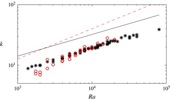
Figure 11. The predicted wavenumber from (5.1) (red dashed), together with data from direct numerical simulations (red circles) of three-dimensional convection (Hewitt et al. Reference Hewitt, Neufeld and Lister2014). The corresponding prediction and results for two-dimensional convection, taken from Hewitt et al. (Reference Hewitt, Neufeld and Lister2013), are shown for comparison (black line and stars).

The result of this argument is thus consistent with the hypothesis that the wavenumber of the interior columnar flow in two-dimensional and three-dimensional high- $Ra$ convection in porous media adopts different scalings because of the different stability properties of the columnar flow. Under this hypothesis, the interior flow is always forced at the boundaries by vigorous mixing of protoplumes (which have a wavenumber ${\sim}Ra$ ), and must coarsen to at least a wavenumber of $k\sim Ra^{1/2}$ in order to transport sufficient heat across the domain. In two dimensions, the interior flow is unstable to a columnar instability that drives coarsening of the columns down beyond this bound to an asymptotic wavenumber $k\sim Ra^{5/14}$ . In three dimensions, the corresponding instability is weaker, and drives coarsening only to an asymptotic wavenumber $k\sim Ra^{1/2}$ . In other words, the instability saturates the upper bound in three dimensions.