2.1. Governing equations

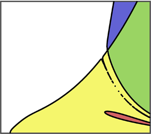
We shall consider the dynamics of an incompressible Newtonian fluid of viscosity $\mu$ and density $\rho$ falling under the influence of gravity down an infinitely long, flexible, impermeable surface inclined at an angle $\beta$ to the horizontal, shown in figure 1. Above the film lies a passive, inviscid gas of constant pressure $p_{0}$, and the surface tension coefficient of the gas–liquid interface is denoted by $\sigma$. We use a rectangular coordinate system $(x,y,z)$ with $x$ measured down the slope (streamwise), $y$ measured in the transverse direction and $z$ measured normal to the slope. As we will exclusively deal with two-dimensional instabilities, we will neglect variation in the $y$ direction. Hence, the instantaneous substrate deflection from its equilibrium position $z=0$ at time $t$ is denoted by $z=\eta (x,t)$, and the instantaneous height of the gas–liquid interface relative to $z=0$ is denoted by $z=h(x,t)$. In this coordinate system, the velocity field in the liquid is $\boldsymbol {u}=(u(x,z,t),0,v(x,z,t))$ with $u$ and $v$ the streamwise and normal velocity components, and acceleration due to gravity takes the form $\boldsymbol {g}=(g\sin \beta ,0,-g\cos \beta )$. The governing equations in the fluid are the two-dimensional Navier–Stokes equations

(2.1a)\begin{gather} u_{t}+uu_{x}+vu_{z} = -\frac{p_{x}}{\rho}+\frac{\mu}{\rho}(u_{xx}+u_{zz})+g\sin\beta, \end{gather}

(2.1b)\begin{gather}v_{t}+uv_{x}+vv_{z} = -\frac{p_{z}}{\rho}+\frac{\mu}{\rho}(v_{xx}+v_{zz})-g\cos\beta, \end{gather}

(2.1c)\begin{gather}u_{x}+v_{z}=0, \end{gather}

where $p$ is the fluid pressure and the subscripts denote partial derivatives. The boundary conditions on the liquid air interface are the kinematic condition and normal and tangential stress balances, which can be written as

(2.2a)\begin{gather} h_{t}+uh_{x} = v, \end{gather}

(2.2b)\begin{gather}(1-h_{x}^{2})(u_{z}+v_{x})+4h_{x}v_{z} = 0, \end{gather}

(2.2c)\begin{gather}-(p-p_{0})+2\mu\left(\frac{1+h_{x}^{2}}{1-h_{x}^{2}}\right)v_{z} = \frac{\sigma h_{xx}}{(1+h_{x}^{2})^{3/2}}, \end{gather}

and it is understood that they are evaluated at $z=h(x,t)$. To arrive at these, the incompressibility condition (2.1c) has been used to simplify (2.2b), and subsequently (2.2b) to simplify (2.2c). These are the typical boundary conditions for a free surface with constant surface tension used for fluid films, and the derivation of which can be seen in, for example, Matar et al. (Reference Matar, Craster and Kumar2007) and Tseluiko & Papageorgiou (Reference Tseluiko and Papageorgiou2006).

Figure 1. Schematic of the problem.

Next we consider the flexible wall. The physical model we will use is shown schematically in figure 2, and was first described in Carpenter & Garrad (Reference Carpenter and Garrad1985) to model actual coatings used by Kramer (Reference Kramer1957). To gain insight into the origin of the terms in a linear wall equation proposed by Carpenter & Garrad (Reference Carpenter and Garrad1985), and also to include the fluid's viscous traction (not present in Carpenter & Garrad (Reference Carpenter and Garrad1985)), we start with a nonlinear model that includes all the relevant physics and then simplify it using the reasonable assumption that longitudinal deflections are much smaller than transverse ones. This in turn provides a modified version of the linear wall equation used in Carpenter & Garrad (Reference Carpenter and Garrad1985). This derivation is included in appendix A.

Figure 2. Schematic representation of the flexible wall model. An elastic sheet of thickness $b$ lies above a rigid surface and backed by an array of springs embedded in a fluid. The distance between springs is much smaller than any instability wavelength, enabling a continuum description.

We will assume the surface of the compliant wall backing to be a two-dimensional inextensible elastic sheet of infinite length (in $x$ and $y$ directions), which is isotropic, and impermeable. Assume that it is thin enough for the longitudinal tension $T$ to be approximately constant across its thickness. It is supported a distance $h_{s}$ above a rigid surface by an array of springs each of stiffness $K$, with a fluid also backing the elastic plate, its motion unaffected by the presence of the springs. Provided the wavelengths of any instabilities considerably exceed the distance between the springs, we can assume the effect of the springs on the plate can be modelled as a continuous elastic foundation of stiffness $K$ for motion in the $z$ direction. We will also assume the presence of damping in the $z$ direction. The linear (in $\eta$) model equation we will use for the substrate deflection $\eta (x,t)$ is given by (see appendix A)

(2.3a)\begin{equation} \rho_{w}b\eta_{tt}+D\eta_{t}-T\eta_{xx}+B\eta_{xxxx}+K\eta=p_{s}-p+2\mu(v_{z}-\eta_{x}(u_{z}+v_{x})), \end{equation}

where $\rho _{w}$ is the plate density, $b$ is the plate thickness, $D$ is the damping coefficient, $T$ is the tension, $B$ is the flexural rigidity, $p_{s}$ is the substrate pressure on the back of the plate provided by the substrate fluid, and all fluid dynamical variables on the right-hand side are evaluated on the substrate, $z=\eta (x,t)$. The case of a viscous and interactive fluid substrate can and has been considered just as in Carpenter & Garrad (Reference Carpenter and Garrad1985), but the two interesting limits of (i) zero substrate viscosity; and (ii) $h_{s}\ll (\text {film thickness})$ can be shown to be equivalent to modifying the wall parameters $A_{D}$ and $A_{I}$ (which we define in § 2.2) while keeping $p_{s}$ constant throughout. Thus, for simplicity, we shall assume $p_{s}$ is constant, determined by the constant height solution, and corresponding to a passive substrate fluid.

Equation (2.3a) is almost identical to that of Carpenter & Garrad (Reference Carpenter and Garrad1985), except for the appearance of normal viscous wall traction from the fluid on the plate: the terms proportional to $\mu$ on the right-hand side. The wall equations used by Halpern & Grotberg (Reference Halpern and Grotberg1992), and subsequently Matar et al. (Reference Matar, Craster and Kumar2007) and Matar & Kumar (Reference Matar and Kumar2004, Reference Matar and Kumar2007), retain this term but neglect bending stresses and wall inertia to retain just damping and tension on the left-hand side (with no stiffness). For linear stability analysis, the equations of Matar et al. (Reference Matar, Craster and Kumar2007) and Matar & Kumar (Reference Matar and Kumar2004, Reference Matar and Kumar2007) are a special case of (2.3a) since for small deflections they are identical to (2.3a) but with $\rho _{w}b, B, K$ set to zero. The $\eta _{x}^{2}$ terms in their equations do not enter into their lubrication analysis anyway since they expand only up to $O(\delta )$ in the lubrication parameter, $\delta =\text {film thickness}/\text {wavelength}$. Thus, for thin films, the wall equation above is an extension of the forms used in the literature (Carpenter & Garrad Reference Carpenter and Garrad1985; Matar et al. Reference Matar, Craster and Kumar2007; Matar & Kumar Reference Matar and Kumar2004, Reference Matar and Kumar2007).

In addition to (2.3a), the linearised form of the no-slip condition on the plate surface becomes

(2.3b)\begin{equation} u=0,\quad v=\eta_{t}\quad\textrm{on}\ z=\eta. \end{equation}

In practice, the material properties $\rho _{w}b$ (mass per unit area), $B$ (flexural rigidity), $T$ (tension) and $D$ (damping coefficient) are not all independent, but related, among other quantities, via the Young's modulus, $E$, and the Poisson ratio, $\nu$, of the plate material. The flexural rigidity is given by

(2.4)\begin{equation} B=\frac{Eb^{3}}{12(1-\nu^{2})}.\end{equation}

The damping coefficient can be determined from the damping ratio, $\zeta$, via the relation

(2.5)\begin{equation} D=2\zeta\sqrt{K\rho_{w}b}. \end{equation}

If required, actual values of the above quantities would have to be determined experimentally or found in materials tables.

The steady base flow of the system (2.1a)–(2.1c) along with the conditions (2.2a)–(2.3b), with constant film thickness $h_0$ and no substrate deflection, $\eta =0$, is given by (bars denote base state quantities)

(2.6)\begin{equation} \left.\begin{array}{c@{}} \bar{u}=\dfrac{g\sin\beta}{2\nu}z(2h_{0}-z),\quad \bar{v}= 0,\\ \bar{h} = h_{0},\quad \bar{\eta} = 0, \\ \bar{p} = p_{0}+\rho g\cos\beta(h_{0}-z),\quad \bar{p}_{s} = p_{0}+\rho gh_{0}\cos\beta. \end{array}\right\}\end{equation}

2.2. Non-dimensionalisation of governing equations

Our non-dimensionalisation is identical to that of Floryan et al. (Reference Floryan, Davis and Kelly1987), with velocities scaled by the Nusselt value $u_{m}=\rho g h_{0}^{2}\sin \beta /2\mu$, lengths with the film thickness $h_{0}$, time with $h_{0} / u_{m}$ and pressure fields with typical viscous stresses $\mu u_{m} / h_{0}$ (after a shift by $p_{0}$). Writing

(2.7a–e)\begin{gather} x^{\ast}=\frac{x}{h_{0}},\quad z^{\ast}=\frac{z}{h_{0}},\quad t^{\ast}=\frac{t u_m}{h_0},\quad h^{\ast}=\frac{h}{h_{0}},\quad\eta^{\ast}=\frac{\eta}{h_{0}}, \end{gather}

(2.8a–d)\begin{gather}u^{\ast}=\frac{u}{u_{m}},\quad v^{\ast}=\frac{v}{u_{m}},\quad p^{\ast}=\frac{(p-p_{0})h_{0}}{\mu u_{m}},\quad p_{s}^{\ast}=\frac{(p_{s}-p_{0})h_{0}}{\mu u_{m}}, \end{gather}

casts the Navier–Stokes equations (2.1a)–(2.1c) into (after dropping stars)

(2.9a)\begin{gather} R \left(u_t + u u_x + v u_z\right) = -p_x + u_{xx} + u_{zz} + 2, \end{gather}

(2.9b)\begin{gather}R \left(v_t + u v_x + v v_z\right) = -p_z + v_{xx} + v_{zz} - 2 \cot \beta, \end{gather}

(2.9c)\begin{gather}u_{x}+v_{z} = 0, \end{gather}

where

(2.10)\begin{equation} R = \rho u_{m}h_0 / \mu, \end{equation}

is the Reynolds number. Note that the viscous pressure scaling is appropriate for our study since the zero-Reynolds-number limit can be taken in a straightforward way. Conditions (2.2a)–(2.2b) at the free surface $z=h$ are unchanged, while the normal stress balance (2.2c) becomes

(2.11)\begin{equation} - p + 2 \left( \frac{1 + h_x^2}{1 - h_x^2} \right) v_z = \frac{S h_{xx}}{\left(1 + h_x^2\right)^{3/2}},\end{equation}

where $S=\sigma / \mu u_{m}$ measures the ratio of capillary forces to inertial forces (it is an inverse Weber number). We note that the surface tension parameter $S$ can be written as $S=K_a R^{-2/3}(\frac {3}{2}\sin \beta )^{-1/3}$, where $K_a=(3\rho \sigma ^3/g\mu ^4)^{1/3}$ is the Kapitza number – see Floryan et al. (Reference Floryan, Davis and Kelly1987) for example – this is used in code validation comparisons with Floryan et al. (Reference Floryan, Davis and Kelly1987).

The conditions on the wall $z=\eta$ become

(2.12a)\begin{gather} u=0,\quad v=\eta_{t}, \end{gather}

(2.12b)\begin{gather}A_I \eta_{tt} + A_D \eta_t - A_T \eta_{xx} + A_B \eta_{xxxx} + A_K \eta = p_s - p + 2 \left( v_z - \eta_x \left( u_z - v_x \right) \right), \end{gather}

where five additional dimensionless groups emerge, $A_{I}$, $A_{D}$, $A_{T}$, $A_{B}$, $A_{K}$, and are defined by

(2.13a)\begin{gather} A_{I} = \frac{\text{wall inertia}}{\text{viscous stress}} = \frac{\rho_{w}bu_{m}^{2}}{h_{0}} \,\, \frac{h_{0}}{\mu u_{m}} = \rho_w b u_m / \mu, \end{gather}

(2.13b)\begin{gather}A_{D} = \frac{\text{damping}}{\text{viscous stress}} = D u_{m} \,\, \frac{h_{0}}{\mu u_{m}} = \frac{D h_{0}}{\mu}, \end{gather}

(2.13c)\begin{gather}A_{T} = \frac{\text{wall tension}}{\text{viscous stress}} = \frac{T}{h_0} \,\, \frac{h_{0}}{\mu u_{m}} = \frac{T}{\mu u_m}, \end{gather}

(2.13d)\begin{gather}A_{B} = \frac{\text{flexural rigidity}}{\text{viscous stress}} = \frac{B}{h_0^3} \,\, \frac{h_{0}}{\mu u_{m}} = \frac{B}{h_0^2 \mu u_m}, \end{gather}

(2.13e)\begin{gather}A_{K} = \frac{\text{spring stiffness}}{\text{viscous stress}} = K h_0 \,\, \frac{h_{0}}{\mu u_{m}} = \frac{K h_0^2}{\mu u_m}. \end{gather}

Note that we have chosen the same time scales for the fluid and wall equations in order to ensure the most general fluid-structure interaction. It then follows that in situations where the wall time scales are much larger than the fluid ones, the parameter $A_I$ in our model will be small (indeed it can be set to zero). With the above scalings the dimensionless base flow becomes

(2.14a–d)\begin{gather} \bar{u} = z(2-z),\quad \bar{v} = 0,\quad \bar{h} = 1,\quad \bar{\eta} = 0, \end{gather}

(2.15a,b)\begin{gather}\bar{p} = 2 \cot \beta (1-z),\quad \bar{p}_{s} = 2\cot\beta. \end{gather}

4.1. Wall parameters and surface tension of $O (1)$

In such cases $S$ and all tilde parameters in (4.3) tend to zero as $\alpha \to 0$, providing the purely imaginary quantity

(4.5)\begin{equation} c_1 = \left(\frac{8}{15} R - \frac{2}{3} \cot\beta + \frac{4}{3 A_{K}} \left(\cot \beta \right)^2 \right) \textrm{i}.\end{equation}

The stability boundary is given by

(4.6)\begin{equation} R=R_c= \frac{5}{4} \cot \beta - \frac{5 (\cot \beta)^2}{2 A_K},\end{equation}

with instability if $R>R_c$. The only wall parameter present in this result is the stiffness $A_K$, and we see immediately that the rigid wall result emerges for $A_K\gg 1$, as expected. The result (4.6) shows that stiffness induces long-wave instability in the sense that, for any finite $A_K$ and a given angle $\beta$, the critical Reynolds number $R_c$ decreases relative to that of a rigid wall. In addition, as $A_K$ decreases to values smaller than $A_K^* = 2 \cot \beta$, we find instability for all $R$, including $R=0$. Figure 3 shows the neutral curves in the $R$–$A_K$ plane, where the critical stiffness $A_K^* = 2 \cot \beta$ is located on the $R=0$ axis for a given $\beta$ as shown. The additional instability as $A_K$ is decreased is clearly seen. As the plate becomes vertical $\cot \beta \to 0$, hence, the critical Reynolds number decreases to zero for every stiffness, however large, in agreement with the rigid wall case. The figure also includes a neutral curve computed from the Orr–Sommerfeld problem and shown by the dashed curve for the case $\alpha =0.1$ and $\cot \beta =1$. We see that agreement is very good, but this would of course deteriorate as $\alpha$ increases. Such computations are described later where it is seen that short waves can become important unlike the rigid wall case.

Figure 3. Neutral curves in the $R$–$A_K$ plane for various values of $\cot \beta$. Verification of the numerical solution is also given by the dashed line for $\alpha = 0.1$, with the accuracy improving as $\alpha \to 0$.

4.2. Inclusion of damping, $\tilde {A}_D = O(1)$

Inspection of (4.3) and (4.4a–e) shows that apart from $A_K$ which is of order one, the next largest effect is due to the damping, $\tilde {A}_D=\alpha A_D$. Here we investigate its effect in the long-wave regime by assuming $\tilde {A}_D=O (1)$ with all other tilde parameters set to zero. In a spring/damper system like the one modelled here, damping controls the dissipation of energy in the system. Underdamped systems oscillate and overdamped ones return to the base state monotonically; coupling this with the fluid dynamics and interfacial perturbations is useful in understanding the fluid-structure instability mechanisms. Mathematically, it is also seen from (4.3) that, for $\alpha \ll 1$ the tension $\tilde {A}_T$, rigidity $\tilde {A}_B$ and inertia $\tilde {A}_I$ just contribute to a renormalisation of the stiffness $A_K$, whereas the inclusion of damping implies that $c_{1r} \neq 0$.

The effect of damping on neutral stability curves analogous to figure 3, is depicted in figure 4 for the fixed angle $\beta =(\rm \pi) /4$. Since $\tilde {S} = \tilde {A}_I = \tilde {A}_T = \tilde {A}_B = 0$, (4.3) gives

(4.7)\begin{equation} c_{1i}= \frac{8}{15} R - \frac{2}{3} \cot\beta + \frac{4(\cot\beta)^2 A_K}{3 \left( A_K^2 + 4\tilde{A}_D^2 \right)}. \end{equation}

It is clear from (4.7) that $\tilde {A}_D$ has a stabilizing effect, and interestingly an island of stability emerges for sufficiently small $R<(5/4)\cot \beta$ and $A_K$, as seen in figure 4 for $\tilde {A}_D=0.4$. More precisely, setting $R=0$ in (4.7) shows that $c_{1i}=0$ when $A_K=\cot \beta \pm \sqrt {(\cot \beta )^2-4\tilde {A}_D^2}$, and as long as $\tilde {A}_D\le (1/2)\cot \beta$, there will be a region of inertialess instability when

(4.8)\begin{equation} \cot\beta-\sqrt{(\cot\beta)^2-4\tilde{A}_D^2}<A_K<\cot\beta+\sqrt{(\cot\beta)^2-4\tilde{A}_D^2}.\end{equation}

This instability region disappears when $\tilde {A}_D=(1/2)\cot \beta$, with the neutral curve having a local minimum at $A_K=\cot \beta , R=0$, as seen in figure 4 for the case $\tilde {A}_D=0.5$. As the damping increases, the neutral curve tends to that for a rigid wall for all values of $A_K$ as seen from (4.7) when $\tilde {A}_D\gg 1$. It is worth noting that in the expression (4.3) the last term is due to wall flexibility, and, hence, the rigid wall result follows if any of the wall parameters become large.

Figure 4. Neutral curves in the $A_K$–$R$ plane for various $\tilde {A}_D = \alpha A_D = O(1)$, with $\cot \beta = 1$, $\tilde {S} = \tilde {A}_I = \tilde {A}_T = \tilde {A}_B = 0$.

4.3. Zero stiffness, $A_K=0$

Having $A_K\ne 0$ is critical for the validity of the expansion leading to (4.3); indeed, if the other parameters are not scaled, then the asymptotic expansion breaks down as $A_K\to 0$. This limit is not uninteresting and is comparable to the model used in Matar et al. (Reference Matar, Craster and Kumar2007); hence, for completeness, the alternative asymptotic solution with zero stiffness is included. Expanding as in (4.1a,b), we now find that $c_0$ has a non-zero imaginary part (higher-order terms need to be determined and solvability conditions imposed as before). After a lot of algebra we find that

(4.9)\begin{equation} c_0 = 1 + \frac{1}{A_D} \pm \frac{\sqrt{(A_D-b)^2-(b^2-1)}}{A_D},\quad \textrm{where}\ b=1+\frac{2}{3}(\cot\beta)^2>1.\end{equation}

Inspection of the expression under the square root shows that $c_{0i}\ne 0$ if $A_D$ satisfies

(4.10)\begin{equation} b-(b^2-1)^{1/2}<A_D<b+(b^2-1).\end{equation}

It follows that as the plate becomes vertical and $b\to 1+$, admissible damping values get squeezed in a small region around $A_D=1$. On the other hand, as the plate becomes horizontal and $b\to \infty$, we have instability for all $A_D$. For the numerical examples where we typically take $\beta =(\rm \pi) /4$, the instability window is $\frac {1}{3}<A_D<3$.

5.1. Effect of stiffness, $A_K$

The substrate stiffness is studied first as it was found to have the greatest effect among the wall parameters. The growth rate $\omega _i = \alpha c_i$ is shown in figure 5 for the choice of the other parameters $\cot \beta =S=A_D=A_T=A_B=A_I=1$. Figure 5(a) demonstrates that for $A_K$ below a critical value $A_{Kc}\approx 2.60$ the flow is unstable, as predicted qualitatively, but not quantitatively as we shall see, by the long-wave analysis. It also shows that for the special case of zero stiffness the gradient at the origin becomes non-zero and was found to match with the zero stiffness asymptotics of § 4.3. In figure 5(b) we show details of the growth rate in the interval $2<A_K<3$, and find that there is a finite wavenumber instability with $\alpha \approx 0.67$ (the wavelength is approximately 9 times the undisturbed film thickness) when $A_K$ just exceeds $A_{Kc}$. This instability occurs before the long wave one at $\alpha =0$, and as a result the earlier long-wave prediction $A_K^* = 2\cot \beta$ (yielding the value 2 in this case) gives a lower prediction for the critical $A_K$ calculated by considering all wavenumbers.

Figure 5. Growth rate curves for Stokes flow for various $A_K$ indicated on the figure. The other parameters are taken to be $\cot \beta =S=A_D=A_T=A_B=A_I=1$.

5.2. Effect of damping, $A_D$

Here we take $\cot \beta =S=A_K=A_T=A_B=A_I=1$ and consider the effect of $A_D$ on the stability. The results are shown in figure 6 with $A_D$ varying between $0$ and $2$. The overall trends are as expected with an increase in damping leading to flow stabilization. Note that the long-wave analysis as well as results at $R=0$ (omitted for brevity), show that this stabilization is limited by the rigid wall case that derives in the limit $A_D\to \infty$. Conversely, decreasing the damping destabilises the flow as expected, but as seen in figure 6 the critical wavenumber $\alpha$ below which instability is supported is weakly affected. Some interesting mode-crossing behaviour is also found at smaller $A_D$, for example, the curves corresponding to $A_D=0$ and $A_D=0.2$ in figure 6. Looking at $A_D=0.2$ for example, we observe a corner in the $\omega _i$ curve at $\alpha =\alpha _c\approx 0.35$ where two modes cross. Our computations produce results for multiple modes and plots such as figure 6 are constructed by tracking the largest value of $\omega _i$ as $\alpha$ varies. For $A_D=0.2$, long-wave instability arises due to an interfacial mode, also termed first mode in the sequel, for $0<\alpha \lessapprox \alpha _c$, and mode switching takes place at $\alpha _c$ with a wall mode, also termed second mode, becoming more unstable for $\alpha \gtrapprox \alpha _c$. The interfacial mode is characterized by being neutral at $\alpha =0$ and long-wave unstable – see below also. To clarify the switching of the most unstable mode from interfacial to wall mode, we plot them together for values of $A_D$ near $0.2$ (all other parameters as in figure 6), providing data for their growth rates and corresponding phase velocity (note that there is a countable infinity of further modes that are all stable and of no concern in this discussion). The results are shown in figure 7 for $A_D=0.25, 0.2225, 0.2$ in figures 7(a)–7(c), respectively. The interfacial mode is shown in blue and passes through the origin, and the wall mode is shown in red. For the two larger values $A_D=0.25$ and $0.2225$, the second mode is unstable but has a smaller maximum growth rate than the first mode. In addition, the wavespeed of the second mode is always larger than that of the first mode as shown in figure 7(a,b). The value $A_D=0.2225$ provides the damping that causes mode switching as we can see by comparison of figures 7(a) and 7(c) – here, the real and imaginary parts of $c$ are the same at the crossing point. Before swapping, the most unstable mode is also long-wave unstable whereas after swapping the most unstable mode is long-wave stable. It is also interesting to note that the wall mode appears to support larger phase velocities as $\alpha \to 0$, something that is analogous to gravity waves in the long-wave limit; see Whitham (Reference Whitham1999). These waves are always stable since $\omega _i<0$ for the second mode if $\alpha$ is below a critical value. The results for $A_D=0.2$ with $\alpha =0.3$, for instance, provide an interesting example where the most unstable mode travels much faster than the analogous rigid wall mode, something that could be useful in experiments.

Figure 6. Growth rate curves for Stokes flow for various $A_D$ indicated on the figure. The other parameters are $\cot \beta =S=A_K=A_T=A_B=A_I=1$. The curves for $A_D=0$ and $A_D=0.2$ indicate mode crossing at a finite $\alpha$.

Figure 7. Plots of the two most unstable modes: interfacial mode – blue, wall mode – red. (a–c) Show the growth rates $\omega _i$ and (d–f) the corresponding phase velocity $c_r$, for $A_D=0.25$ (a,d), $A_D=0.2225$ (b,e) and $A_D=0.2$ (c,f). The other parameters are $\cot \beta = S = A_T = A_B = A_K = A_I = 1$.

6.1. Numerical methods and code validation

Sections 4 and 5 produced asymptotic solutions for small $\alpha$ but arbitrary $R$, and small $R$ and arbitrary $\alpha$, respectively. The latter analysis indicates that in the presence of wall flexibility the maximally growing waves occur at order one wavenumbers; hence, it is important to extend our stability studies to arbitrary wavenumbers and Reynolds numbers computationally. We briefly describe our numerical methods used to solve the Orr–Sommerfeld eigenvalue problem (3.1) subject to the interfacial conditions (3.2), (3.3), and the wall conditions (3.7), (3.8). The solution is approximated by a truncated series of Chebyshev polynomials of the first kind, in particular, following the $D^{2}$ Chebyshev tau scheme of Dongarra, Straughan & Walker (Reference Dongarra, Straughan and Walker1996). This involves introducing $\chi (z)=({\mbox {d}^{2}}/{\mbox {d}z^{2}}-\alpha ^{2})\phi (z)$, which transforms the single fourth-order equation for $\phi$ into a pair of second-order equations for $\phi$ and $\chi$. We write

(6.1a,b)\begin{equation} \phi(z) = \sum_{n=0}^{N+2}\phi_{n}T_{n}(z),\quad \chi(z) = \sum_{n=0}^{N+2}\chi_{n}T_{n}(z), \end{equation}

where $T_{n}(z)$ is the $n$th Chebyshev polynomial, and $N$ is a measure of the truncation (with $N+3$ polynomials used). Differentiation is performed directly by operating on the $T_{n}$. Hence, substituting into the equations and BCs for $(\phi ,\chi )$ and using the orthogonality properties of the $T_{n}$ (Dongarra et al. Reference Dongarra, Straughan and Walker1996), we can write the system as a finite-dimensional nonlinear eigenvalue problem for $c$,

(6.2)\begin{equation} (c^{2}\boldsymbol{\mathsf{B}}_{2}+c\boldsymbol{\mathsf{B}}_{1}+\boldsymbol{\mathsf{B}}_{0})\boldsymbol{x}= \boldsymbol{0},\quad\mbox{where}\ \boldsymbol{x}=(\phi_{0},\ldots,\phi_{N+2},\chi_{0},\ldots,\chi_{N+2})^{\textrm{T}},\end{equation}

and $\boldsymbol{\mathsf{B}}_{2},\boldsymbol{\mathsf{B}}_{1},\boldsymbol{\mathsf{B}}_{0}$ are $2(N+3)\times 2(N+3)$ matrices with their bottom four rows representing the boundary conditions (3.2), (3.3), (3.7) and (3.8) in turn expressed in terms of the Chebyshev coefficients $\boldsymbol{x}$. Notice that we have a nonlinear $c^{2}$ term in (6.2) which is absent for this method of discretisation for the case of flow down a rigid wall. This nonlinearity is due solely to the inertia of the flexible wall, i.e. the second-order time derivative of $\eta$ in the equation for the wall deflection (2.12b). It appears only through (3.8) as the first term on the left-hand side and is proportional to $A_{I}$, implying that the matrix $\boldsymbol{\mathsf{B}}_{2}$ contains zeros everywhere except for the last row, and $\boldsymbol{\mathsf{B}}_{2}=\boldsymbol{0}$ if $A_{I}=0$. The eigenvalues are computed using the Matlab routines polyeig or eig when $A_I\ne 0$ or $A_I=0$, respectively. Spurious or infinite eigenvalues with unphysical growth rates arise due to the singular rows of the matrices $\boldsymbol{\mathsf{B}}_{2}, \boldsymbol{\mathsf{B}}_{1}$, Dawkins, Dunbar & Douglass (Reference Dawkins, Dunbar and Douglass1998): half the rows of $\boldsymbol{\mathsf{B}}_{1}$ are zero owing to the introduction of $\chi$, and another row is zero owing to boundary condition (3.7), as both $\chi$ and (3.7) are independent of $c$. We ignore these eigenvalues numerically, but the one due to (3.7) is removed entirely by elimination; see McFadden, Murray & Biosvert (Reference McFadden, Murray and Biosvert1990) for details. The numerical results were computed for zero Reynolds number and compared against the analytical results of § 5 for a variety of parameters, with excellent agreement.

The code was validated by comparing computed variations of $c_r$ and $c_i$ with $\alpha$, with their long-wave counterparts presented in § 4. For completeness, a small selection of these checks for values of the stiffness parameter $A_K=0.5, 1, 10$ are presented in figure 8, with $\cot \beta$, $R$ and the other wall parameters set to unity. The computational results are depicted with solid curves and the corresponding long wave ones by the dashed straight lines. Agreement improves as $\alpha$ decreases, as expected, and the results indicate that long-wave theory does a reasonable job for $\alpha \lessapprox 0.1$, at least for this set of parameters. Lastly, the long-wave neutral curves in the $R$–$A_{K}$ plane that were analysed in § 4 can be reproduced by the numerics for small $\alpha$. For instance, in figure 3 the computed neutral curve corresponding to $\cot \beta =1$ and $\alpha =0.1$ is seen to be in very good agreement with the long-wave neutral curve for the whole range of $R$ and $A_K$ considered.

Figure 8. Comparison between computed values (solid lines) of $c_r$ and $c_i$ with the asymptotic long-wave solution (dashed lines) for various stiffnesses $A_{K} = 0.5, 1, 10$ indicated on the figure; also, $R=1$, $A_{I}=A_{D}=A_{T}=A_{B}=1$, $N=50$ and $S=\cot \beta =1$.

6.2. Numerical results

We begin by presenting results for an inclination angle $\beta =(\rm \pi) /4$ for which the critical Reynolds number is $1.25$. Smaller angles and large Reynolds numbers will be considered later. As with the analytical results, we start by varying the stiffness parameter $A_K$ with $A_D, A_T, A_B, A_I$ set to unity. Neutral stability curves in the $\alpha$–$R$ plane are given in figures 9(a) and 9(b) for surface tension parameters $S=1$ and $S=1000$, respectively, the latter being more realistic for water. In both cases the rigid wall results begin to emerge for the largest value of $A_K=5$ (green curves), and we note the additional long-wave destabilization for the $S=1000$ case by the flattening of the curve near the critical $R$. As $A_K$ increases further, the flattened region disappears and a larger critical $R$ is found due to the larger $S$ involved. Figures 9(a) and 9(b) also show that the finite wavenumber instabilities found analytically at $R=0$ are also supported when inertia is present. For both $S=1$ and $S=1000$, we observe islands of long-wave stability when $R$ is small enough, e.g. the neutral curve for $A_K=2.6$ in figure 9(a). Larger $S$ stabilises the flow by shifting the neutral curves to the right to larger values of $R$, as seen in figure 9(b). If the stiffness is removed completely ($A_K=0$, blue curve) the flow becomes unstable to long waves at all Reynolds numbers considered. For large $A_K$, the effect of the interfacial instability is dominant, while for small $A_K$, wall flexibility becomes more important thus explaining the slight effect of $S$ in this limit.

Figure 9. Neutral stability curves in the $\alpha$–$R$ plane as the wall stiffness varies (values of $A_K$ indicated on the plot), and for surface tension values $S=1$ (a) and $S=1000$ (b). Other parameters are $\cot \beta =A_D=A_T=A_B=A_I=1$.

Corresponding growth rates from figure 9(a) are presented in figures 10(a) and 10(b) for $R=0.2$ and $R=3$, respectively, with the stiffness $A_K$ varying between $2.0$ and $2.6$. For $R=0.2$, we observe the long-wave stabilization at the largest $A_K=2.6$ in line with the $R=0$ results of figure 5(b). As inertia increases to $R=3$, however, the long-wave stabilization is lost and the band of unstable waves as well as the maximum growth rate, increase with $R$. At the same time the instability also increases with decreasing stiffness for fixed $R$, as seen in figure 10(b).

Figure 10. Effect of inertia on the growth rates $\omega _i$ as $A_K$ varies (values shown on the plots): (a) $R=0.2$, (b) $R=3$. The other parameters are $\cot \beta =S=A_D=A_T=A_B=A_I=1$.

Next, the effect of the wall damping $A_D$ is investigated for an inclination $\beta =(\rm \pi) /4$, all other parameters set to unity. Results are given in figures 11(a) and 11(b) that show the neutral curves as $A_D$ varies, and representative growth rate curves at $R=1$. From the long-wave expression (4.3) we expect that, for large $A_D$, the solution tends to the rigid wall limit, however, it is not clear from the expansion how the limit is approached and we use computations to explore this. Two things are worth pointing out from the results of figure 11(a). First, for a given Reynolds number below the critical value for a rigid wall, we see that the damping does not fully stabilize the solution but supports a small band of unstable long waves – this can be seen clearly for $A_D=64$ in figure 11(a) at a Reynolds number of $1$ and smaller for example, and is in contrast to the large $A_K$ limit where stabilization occurs at a large but finite $A_K$ (e.g. figure 9a for $A_K=5$). Second, larger $R$ damping is seen to have a stabilizing effect in the sense that it reduces the unstable region in the $\alpha$–$R$ plane; compare the cases $A_D=64$ with $A_D=4$ in figure 11(a), for example, but at the same time note that this effect is non-monotonic in $A_D$ as seen from subsequent curves for $A_D=1$ and $A_D=0.25$. This phenomenon is due to fluid inertia and is not seen at either long waves or zero Reynolds numbers. Figure 11(b) shows the largest computed growth rate versus $\alpha$ for $R=1$; we observe that an increase in damping reduces the maximum growth rate as well as the neutral wavenumber. The results for $A_D\ge 4$ also indicate the presence of a second mode as found at zero Reynolds numbers in § 5, figure 6 for instance.

Figure 11. Stability characteristics as $A_D$ varies. (a) The neutral curves for the parameter set $\cot (\beta )=S=A_T=A_B=A_K=A_I=1$ and (b) the growth rate $\omega _i$ when $R=1$.

The results above show that long-wave instability persists at large $A_D$ for the parameters chosen. Combined with the results of figure 9(a), we can surmise that this instability should in turn disappear as the stiffness $A_K$ is increased. To illustrate some of the characteristics and, in particular, to show underlying mechanisms such as mode crossings, we take $A_D=0.32$, $A_K=5$ and all other parameters equal to unity. At the chosen parameter values we also find the coexistence of unstable interfacial and wall modes over a large range of wavenumbers. Figure 12(a) shows the neutral curves in the $\alpha$–$R$ plane for the range $0\le R\le 4$. We see that there are two modes present, the usual rigid wall interfacial mode with a critical Reynolds number for long waves, along with a second wall mode that has two branches for large $R$ (the upper branch grows with $R$ while the lower one decays as $R$ increases). An interesting finding from these results is that at small Reynolds numbers wall flexibility can destabilize the flow by reducing the critical Reynolds number and inducing a finite wavenumber instability. This can be seen from figure 12(a) where the critical Reynolds number is reduced to approximately $0.332$ and the first wavenumber that becomes unstable just above critical has $\alpha \approx 0.549$. For completeness in figure 12(b), we also present growth rates. Figure 12(b) fixes $R=0.5$ (depicted by the vertical dashed line in figure 12a), and shows the effect of varying $A_D$ between $0.1$ and $0.5$ on the most dominant mode. The presence of the two modes is seen in the plots and the finite wavenumber instability due to the wall mode is clear. The maximum growth rate increases as $A_D$ is decreased but the maximally unstable wavenumber varies weakly. We also note that at much higher $R$ there is another shear instability mode and the coexistence of all three modes and their relative growth rates are considered later.

Figure 12. (a) A neutral stability diagram; and (b) growth rate curves, each showing the presence of two unstable modes, for the parameter set: $A_K = 5$, $\cot (\beta )=S=A_T= A_B=A_I =1$. The growth rate curves also show the effect of increasing the damping ($A_{D}$) on the two modes. (a) $A_D=0.32$; (b) $R=0.5$.

6.3. Instabilities at high Reynolds numbers

It is well known in falling film flows that at higher Reynolds numbers shear modes of instability enter in addition to the interfacial mode that is prominent at lower values of $R$; see Floryan et al. (Reference Floryan, Davis and Kelly1987). Our model and computational tools enable us to carry out a detailed investigation of the effect of wall flexibility on such modes, and indeed the interaction and competition between modes resulting from the three different physically supported instabilities. We will mostly present our results in the form of neutral stability curves in the $R$–$\alpha$ plane. Due to the large number of parameters, preliminary computations were carried out to identify which wall parameters are the most important, and in what follows we consider the effect of the stiffness parameter $A_K$ with a moderate amount of damping also present with $A_D=10$. The case computed has an inclination angle $\beta =4^{\circ }$ in order to extend the results of Floryan et al. (Reference Floryan, Davis and Kelly1987) to include wall flexibility. Representative results are given in figure 13 with the wall stiffness parameter $A_K$ varying from $10^5$ in panel (a) to $10$ in panel (f). All other wall parameters and surface tension are set to unity.

Figure 13. Neutral curves for the different modes in the $R$–$\alpha$ plane as the stiffness $A_K$ varies. The parameters are $\beta = 4^{\circ }$, $A_D = 10$ with all remaining parameters set to $1$. The U and S labels refer to unstable and stable regions, respectively. (a) $A_K = 10^5$ (almost rigid); (b) $A_K = 10^4$; (c) $A_K = 10^3$; (d) $A_K = 10^3$, enlargement of dotted area in (c); (e) $A_K = 10^2$; (f) $A_K = 10$ (highly flexible).

For large stiffness $A_K=10^5$, the wall is almost rigid. The results of figure 13(a) contain three different modes as labelled. These include the typical interfacial and shear mode neutral curves computed by Floryan et al. (Reference Floryan, Davis and Kelly1987), and in addition a mode due to wall flexibility; the first mode is a long-wave interfacial one supporting instability at relatively small $R$, whereas the second is a shear mode that appears at larger $R\approx 5\times 10^3$ – the shear mode was not seen in all previous results presented because the range of Reynolds numbers plotted was not large enough. The resulting plot is in full agreement with Floryan et al. (Reference Floryan, Davis and Kelly1987) once differences in non-dimensionalisation are accounted for. The wall mode enters at a critical $R\approx 5\times 10^4$, and as $A_K$ increases this critical value also increases. It is described in more detail below for lower stiffnesses when it becomes more dominant.

Reducing the stiffness by an order of magnitude to $A_K=10^4$ produces the results of figure 13(b). Several effects are notable: (i) the wall mode enters at a lower critical Reynolds number $R\approx 6\times 10^3$, and enhances the band of unstable wavenumbers to include shorter waves at lower Reynolds numbers; (ii) the shear mode becomes a little more stable entering at a critical $R\approx 6\times 10^3$, and at the same time narrowing its band of unstable wavenumbers; (iii) a break is observed in the interfacial mode with additional neutral curves appearing – this is due to an interaction between the different modes and is investigated fully for later plots by using an energy decomposition analysis.

The interaction of modes and the splitting of the interfacial mode found at large $A_K$, becomes clearer as $A_K$ decreases to $10^3$ as shown in figure 13(c). The wall mode becomes unstable at lower values of $R\approx 10^3$, and the intricate interaction behaviour in the lower right-hand corner of the figure (identified by a dashed rectangular border) becomes clearer in the enlargement given in figure 13(d). The shear mode is the lowest feature seen in the figure, and the flow is unstable everywhere. There are either one or two unstable modes in different parts of the depicted region. For example, fixing $R=2\times 10^4$ and varying $\alpha$, the number of unstable modes alternate between one and two every time a neutral curve is crossed.

In the last two figures 13(e) and 13(f) we follow the change in the neutral curves as $A_K$ is decreased to $100$ and $10$, respectively, the last case comprising the most flexible wall considered in this study. For $A_K=100$, the two main modes, namely the interfacial and wall mode, are still prominent, the former at smaller $R$ and $\alpha$ and the latter at moderate $R$ and order one $\alpha$, but the results indicate further mode interaction and switching. For example, considering a fixed value $R=500$ as $\alpha$ is increased from zero we initially encounter instability due to the interfacial mode, followed by a small window of stability before additional modes enter at moderate $\alpha$, and eventually one wall mode remains at higher wavenumbers (complete stabilisation takes place at short waves due to surface tension). The presence of an interfacial mode at small $R$, coupled with a complete stability of the system at values of $R$ below a critical value, cease to exist for higher wall flexibility as illustrated in the results of figure 13(f) for $A_K=10$. In decreasing $A_K$ from $100$ to $10$, the merged interfacial and wall modes evolve to give the uppermost neutral curve, resulting in long-wave instability at small Reynolds numbers including $R=0$, consistent with figure 5. At higher $R$ an additional mode enters with the flow remaining unstable everywhere to the right of the uppermost neutral curve that extends back to $R=0$. In figures 13(e) and 13(f) the horizontal dashed lines drawn through $\alpha =1$ indicate the parameters over which we carry out an energy analysis that helps us identify the physical origin of the different instabilities as the Reynolds number is increased. This analysis and the results are presented next.

6.4. Energy analysis

Due to the complexity of neutral stability plots such as those in figure 13, we provide results of an energy decomposition of different terms in the perturbation equations in an effort to link particular modes with their physical origin. We proceed as in the energy decomposition analysis of Kelly et al. (Reference Kelly, Goussis, Lin and Hsu1989) for rigid wall falling films. We start with the linearised equations for the perturbations in primitive variables and take inner products to derive an equation for the evolution of the kinetic energy of the system integrated over the periodic domain. The length of the period is taken to be $L = 2 {\rm \pi}/ \alpha$, thus allowing direct comparison to the neutral curves. The surface and wall parameters enter the equation through the evaluation of integrals at the boundaries. Details of the derivation are given in appendix B. The final result we need here is

(6.3)\begin{equation} \frac{1}{2}\frac{\partial\mathcal{E}}{\partial t} = {DISSI} + {REYNS} + {SURFS} + {WALLS} + {DAMP} + {WALLH}, \end{equation}

where the energy $\mathcal {E}\ge 0$ is given by

(6.4)\begin{gather} \mathcal{E}=E_{KIN} +E_{SURF} + E_{WALL} + E_{HYD}, \end{gather}

(6.5)\begin{gather}E_{KIN} = R\iint_{\Omega} (u^2+v^2) \,\textrm{d} x\,\textrm{d} z, \end{gather}

(6.6)\begin{gather}E_{SURF} = S\int_{-L/2}^{L/2} h_x^2 \,\textrm{d} x, \end{gather}

(6.7)\begin{gather}E_{WALL} = \int_{-L/2}^{L/2} \left(A_I \eta_t^2 + A_T \eta_x^2 + A_B \eta_{xx}^2 + A_K \eta^2\right) \textrm{d} x, \end{gather}

(6.8)\begin{gather}E_{HYD} = 2 \cot\beta \int_{-L/2}^{L/2} h^2 \,\textrm{d} x, \end{gather}

where $E_{KIN}$ represents the kinetic energy within the fluid, $E_{SURF}$ the energy stored in the deformed surface due to surface tension, $E_{WALL}$ the energy contribution due to wall flexibility and $E_{HYD}$ denotes the hydrostatic potential energy. The right-hand side includes the following terms that control the rate of change of the total energy:

(6.9)\begin{gather} {DISSI} = - \iint_{\Omega} \left( \left| \boldsymbol{\nabla} u \right|^2 + \left| \boldsymbol{\nabla} v \right|^2 \right) \textrm{d} x\,\textrm{d} z, \end{gather}

(6.10)\begin{gather}{REYNS} = - 2 R \iint_{\Omega} u v \left( 1 - z \right) \textrm{d} x\,\textrm{d} z, \end{gather}

(6.11)\begin{gather}{SURFS} = \int_{-L/2}^{L/2} u \left( u_z - v_x \right) |_{z=1} \,\textrm{d} x, \end{gather}

(6.12)\begin{gather}{WALLS} = - \int_{-L/2}^{L/2} u \left( u_z + v_x \right) |_{z=0} \,\textrm{d} x, \end{gather}

(6.13)\begin{gather}{DAMP} = - A_D \int_{-L/2}^{L/2} \eta_t^2 \,\textrm{d} x, \end{gather}

(6.14)\begin{gather}{WALLH} = 2 \cot(\beta) \int_{-L/2}^{L/2} \eta v \,\textrm{d} x. \end{gather}

The viscous dissipation is denoted by DISSI and the Reynolds stress by REYNS. The rate of work done by shear on the surface and the wall enter as SURFS and WALLS, respectively. The damping term in the wall model contributes to the equation with the stabilising DAMP term and, finally, WALLH denotes a term originating from the work done by the hydrostatic pressure on the wall; see appendix B.

Picking a wavenumber $\alpha$ and other system parameters, the linear stability results (eigenvalue-eigenfunction pairs) provide numerical values of each term on the right-hand side of (6.3). In what follows we present results for $\alpha =1.0026$ and follow the instability as the Reynolds number increases along the dashed lines in figures 13(e) and 13(f), with the corresponding energy decomposition results given in figures 14 and 15, respectively.

Figure 14. A growth rate plot (a) and the energy decompositions (b–d), see (6.3), of the three unstable eigensolutions for the case $\alpha = 1.0026$, $\beta = 4^{\circ }$, $A_K = 100$ and $A_D = 10$ with all other parameters set to unity.

Figure 15. Plots showing the growth rate (a) and energy decompositions (b,c), see (6.3), of the two unstable eigensolutions for the case $\alpha = 1.0026$, $\beta = 4^{\circ }$, $A_K = 10$, $A_D = 10$ with all other parameters set to $1$.

Results for $A_K=10^2$ are given in figure 14 for fixed $\alpha =1.0026$ as $R$ varies. Figure 14(a) shows the growth rates of the three most unstable modes for $R$ between $1$ and $2\times 10^3$ (we restricted the range of $R$ in order to make the results clearer). The modes are depicted by different symbols, with the corresponding energy decomposition of each mode provided in the accompanying plots as follows: mode 1 with square symbol is analysed in figure 14(b); mode 2 with circles is analysed in figure 14(c); and mode 3 with triangles in figure 14(d). In the energy decomposition panels, each term from the right-hand side of the energy equation (6.3) is included by a different colour and identified in the legend. The black curve denoted by TOTAL provides the sum of all terms, i.e. the right-hand side of (6.3). As expected, the neutral Reynolds number predicted by this curve is identical to that predicted by the corresponding growth rate of each mode in figure 14(a). In all cases the viscous dissipation (DISS) and wall damping (DAMP) are negative for all $R$ as expected, and play a significant role on the overall stability characteristics. At smaller $R$ they act to thwart growth due to other effects ensuring that a finite $R$ is needed for instability. Starting with mode 1 in figure 14(b), we see that instability is mainly associated with Reynolds stresses, surface stresses and wall stresses. As these increase with $R$, viscous dissipation and wall damping also increase and delay the appearance of instability. The instability is constrained to a small window in $R$ mainly due to the significant decrease of the Reynolds stresses from around $R\approx 7\times 10^2$. We conclude that instability for this mode is due to Reynolds and wall stresses (yellow and red curves, respectively).

For mode 2 (circles), energy growth at smaller $R$ is dominated by Reynolds and wall stresses as seen in figure 14(c). Other effects are stabilizing and in particular a sizeable viscous dissipation ensures negative growth rates. As $R$ increases to values between $10^2$ and $10^3$, Reynolds and wall stresses peak to maximum values before decaying significantly by $R\approx 10^4$. At the same time the surface shear stress term enters to provide energy growth, and coupled with weaker viscous dissipation and wall damping, an instability ensues as indicated in the figure. This instability is mainly due to the mechanism of energy growth due to surface shear stresses (SURFS, blue curve).

Mode 3 (triangular symbols) in figure 14(d) has quite different energy decomposition. At smaller $R$, energy growth is entirely due to wall stresses (red curve), but viscous dissipation dominates providing stability. As $R$ increases both wall stresses and Reynolds stresses decrease further to reach local negative minima, until $R\approx 7\times 10^2$ when they both provide energy growth; in addition, the hydrostatic pressure wall mode (WALLH) produces energy growth beyond $R\approx 10^3$. As a result, and due to the large energy growth of the Reynolds stresses, the growth rate increases substantially as seen in figure 14(a).

Finally, we present results for the smallest value $A_K=10$ considered here. As in figure 14, we fix $\alpha =1.0026$ and look at the energetics of the dominant modes as $R$ is varied along the dashed line in figure 13(f). This case is particularly interesting since instability is supported for all $R$, even $R=0$, unlike the other $A_K$ cases described. The presentation of the results in figure 15 follows that above. Only two unstable modes exist for $\alpha =1.0026$ and $0\le R\le 10^4$, and their growth rates as $R$ varies are depicted in figure 15(a). The energy decomposition of mode 1 (square symbols) is included in figure 15(b) and the corresponding data for mode 2 (circles) appear in figure 15(c). The results show that for small $R$ (including near zero) mode 1 is driven by the work done by the hydrostatic pressure on the wall (WALLH, the light blue curve) and the wall shear stresses (WALLS, red curve). At larger $R$ (higher than $25$, approximately) the Reynolds stresses dominate while the effects of SURFS and WALLH level out to approximate equal values and so the physical mechanism responsible for instability switched from boundary effects to bulk Reynolds stresses. The surface shear stresses play no role in the dynamics explaining why this mode is not observable in the absence of wall elasticity. We also note that the viscous dissipation and wall damping terms suppress the instability but are not high enough to stabilize the flow at any values of $R$ considered. The energetics of mode 2 (circles in figure 15a) follow very similar trends to those of mode 2 of the larger $A_K=10^2$ case shown in figure 14(c), and so we can conclude that they are a continuation of one another and we do not need to discuss it further.