


1 Introduction
The process of fuel injection in aeroengine combustion chambers typically relies on the azimuthal component of mean flow with swirl to enhance flame anchoring via appropriate recirculation zones that promote mixing (Candel et al.
Reference Candel, Durox, Schuller, Bourgouin and Moeck2014). Inside the combustion chamber, for sufficiently high rotation rates, this could yield complex hydrodynamic structures (see Gallaire & Chomaz Reference Gallaire and Chomaz2003; Loiseleux & Chomaz Reference Loiseleux and Chomaz2003; Liang & Maxworthy Reference Liang and Maxworthy2005; Gallaire et al.
Reference Gallaire, Ruith, Meiburg, Chomaz and Huerre2006) that may enhance flame stabilization (e.g. Huang & Yang Reference Huang and Yang2009). However, there is also the distinct possibility of resonant coupling between such hydrodynamic structures with the lower-frequency acoustic waves further upstream, inside any of the multiple swirler ducts of a modern aeroengine fuel injection system. In fact, instabilities in swirl-stabilized combustion chambers, which are sometimes manifested in the form of three-dimensional helical structures with a precessing vortex core (e.g. Huang & Yang Reference Huang and Yang2009), have often been traced to conditions inside the injector tube (see e.g. figure 3c in Candel et al.
Reference Candel, Durox, Schuller, Bourgouin and Moeck2014). In this work, the compressible rotating Hagen–Poiseuille flow (CRHPF) with variable mean density is used as a model for the near-sonic-speed premixed flow inside such air swirler ducts. In the air-assisted atomizer designs, for example, high-velocity air jets are introduced to aid in the fuel atomization process, especially at the lower fuel flow rates when the corresponding flow Mach numbers could be potentially high enough (perhaps close to choked; see e.g. Lefebvre & Ballal Reference Lefebvre and Ballal2010) for compressibility effects to be significant. The stratification in mean density of such flows could be a result of imperfect internal mixing of the multiple fuel and air streams, the former also likely to be differentially heated, a direct consequence of modern multi-swirler designs (e.g. the General Electric TAPS; see Mongia Reference Mongia2003), where the main air stream gets intermixed with multiple secondary fuel streams and also fuel vapours, normally at different temperatures (e.g. Swaminathan & Bray Reference Swaminathan and Bray2011). Typically, such injection systems are required to adapt over wide ranges of fuel flow rates, yielding variations in flow Mach and Reynolds numbers, forcing a stable CRHPF to potentially transition into a state of convective instability, perhaps even yielding an absolutely unstable state at higher
 $Re$
and rotation rates. In this work, we analyse these different stability states via specifically focusing on the roles played by the various competing disturbance energy mechanisms.
$Re$
and rotation rates. In this work, we analyse these different stability states via specifically focusing on the roles played by the various competing disturbance energy mechanisms.
The study of instabilities in swirling flow has a long history, tracing back to the linear stability analyses of Rayleigh and Synge (Rayleigh Reference Rayleigh1916; Synge Reference Synge1933), yielding the classical Rayleigh–Synge criterion, which showed a solid-body swirling flow with no axial and radial velocity components to be linearly stable at all swirl levels. Later studies included the missing axial velocity component and were further extended for non-axisymmetric disturbances (see Howard & Gupta Reference Howard and Gupta1962; Lessen & Paillet Reference Lessen and Paillet1974; Leibovich & Stewartson Reference Leibovich and Stewartson1983), all of which essentially concluded that increased swirl improves the flow stability (see also Wang & Rusak Reference Wang and Rusak1996). This directly contrasts with the observation that vortex breakdown in swirling flow is reached as the swirl crosses a certain threshold (see e.g. Leibovich Reference Leibovich1984; Escudier Reference Escudier1988; Sarpkaya Reference Sarpkaya1995). Starting with Wang & Rusak (Reference Wang and Rusak1996), a different approach for swirling flows in finite-length pipes was proposed to connect the vortex breakdown phenomenon with flow instability, which for the first time clearly demonstrated that beyond a critical swirl, the flow becomes linearly unstable, manifested via an axisymmetric vortex breakdown. It has been subsequently argued that for a swirling flow in a ‘short-length’ pipe with a vortex generator present, the overall flow dynamics is strongly coupled to specific inlet and exit conditions, which invalidates a classical stability analysis (see e.g. Wang & Rusak Reference Wang and Rusak1996; Wang et al. Reference Wang, Rusak, Gong and Liu2016).
A rotating Hagen–Poiseuille flow (RHPF) with a non-uniform axial speed has also been frequently used to model the mean flow inside a pipe, which by virtue of being a fully developed profile is independent of any effects from the pipe ends. Moreover, the absence of a jet-like or wake-like mean profile resembling that of classical vortex flows points to the difficulty in linking any vortex breakdown of RHPF with its instability, which is also something not pursued here. In practice, such profiles are applicable to a ‘narrow pipe’, where the pipe length is typically an order of magnitude larger than the pipe diameter (see e.g. the experimental set-up of Shrestha et al.
Reference Shrestha, Parras, Pino, Sanmiguel-Rojas and Fernandez-Feria2013) or the length is comparable to the wavelength of the most dominant stability mode (see e.g. Sugimoto Reference Sugimoto2010). The dimensions of typical swirler ducts, as discussed above, are such that they tend to qualify as narrow tubes and hence RHPF is a good model for the swirling flow inside. In contrast, in a full-length combustion chamber, for example, this is unlikely to be a good model as has been already demonstrated by Wang & Rusak (Reference Wang and Rusak1996) and Wang et al. (Reference Wang, Rusak, Gong and Liu2016). Linear stability analysis has been used to predict the breakdown of such swirling pipe flows, using both temporal (e.g. Pedley Reference Pedley1968, Reference Pedley1969; Mackrodt Reference Mackrodt1976; Cotton & Salwen Reference Cotton and Salwen1981; Maslowe & Stewartson Reference Maslowe and Stewartson1982) and spatial models (Fernandez-Feria & del Pino Reference Fernandez-Feria and del Pino2002), where the otherwise unconditionally linearly stable pipe flows are shown to be unstable to non-axisymmetric perturbations once swirl is introduced. For higher rotation rates, i.e. at small Rossby numbers
 $\unicode[STIX]{x1D716}$
(inverse of the swirl parameter
$\unicode[STIX]{x1D716}$
(inverse of the swirl parameter
 $L$
), the critical Reynolds number
$L$
), the critical Reynolds number
 $Re_{c}$
for convective instability appears to be surprisingly low (compared to flows that use vortex models), and becomes independent of
$Re_{c}$
for convective instability appears to be surprisingly low (compared to flows that use vortex models), and becomes independent of
 $\unicode[STIX]{x1D716}$
once a certain rotation rate is exceeded (see Fernandez-Feria & del Pino Reference Fernandez-Feria and del Pino2002). Beyond the appearance of the convectively unstable regime, spatial stability analysis has been used by e.g. Fernandez-Feria & del Pino (Reference Fernandez-Feria and del Pino2002) to trace the boundary of convective to absolute transition via the well-known Briggs–Bers theory (see Briggs Reference Briggs1964; Bers Reference Bers1983), bypassing a potentially more-involved spatio-temporal analysis (e.g. Olendraru et al.
Reference Olendraru, Sellier, Rossi and Huerre1999). Their results show that at the incompressible limit, for a given
$\unicode[STIX]{x1D716}$
once a certain rotation rate is exceeded (see Fernandez-Feria & del Pino Reference Fernandez-Feria and del Pino2002). Beyond the appearance of the convectively unstable regime, spatial stability analysis has been used by e.g. Fernandez-Feria & del Pino (Reference Fernandez-Feria and del Pino2002) to trace the boundary of convective to absolute transition via the well-known Briggs–Bers theory (see Briggs Reference Briggs1964; Bers Reference Bers1983), bypassing a potentially more-involved spatio-temporal analysis (e.g. Olendraru et al.
Reference Olendraru, Sellier, Rossi and Huerre1999). Their results show that at the incompressible limit, for a given
 $Re$
, the transition from convective to absolute instability occurs at rotation rates higher than when the convective instability first appears, but only if the rotation rate exceeds a minimum
$Re$
, the transition from convective to absolute instability occurs at rotation rates higher than when the convective instability first appears, but only if the rotation rate exceeds a minimum
 $L$
(or is below a maximum
$L$
(or is below a maximum
 $\unicode[STIX]{x1D716}_{max}$
), irrespective of
$\unicode[STIX]{x1D716}_{max}$
), irrespective of
 $Re$
. As the solid-body rotation rate is further increased so that
$Re$
. As the solid-body rotation rate is further increased so that
 $\unicode[STIX]{x1D716}$
reduces by approximately one order of magnitude from
$\unicode[STIX]{x1D716}$
reduces by approximately one order of magnitude from
 $\unicode[STIX]{x1D716}_{max}$
to
$\unicode[STIX]{x1D716}_{max}$
to
 $\unicode[STIX]{x1D716}_{min}$
, the convectively unstable zone now disappears and the flow transitions directly from a stable to an absolutely unstable state at critical Reynolds number
$\unicode[STIX]{x1D716}_{min}$
, the convectively unstable zone now disappears and the flow transitions directly from a stable to an absolutely unstable state at critical Reynolds number
 $Re_{t}=Re_{c}$
, essentially independent of
$Re_{t}=Re_{c}$
, essentially independent of
 $\unicode[STIX]{x1D716}$
for
$\unicode[STIX]{x1D716}$
for
 $\unicode[STIX]{x1D716}<\unicode[STIX]{x1D716}_{min}$
(see Fernandez-Feria & del Pino Reference Fernandez-Feria and del Pino2002; Shrestha et al.
Reference Shrestha, Parras, Pino, Sanmiguel-Rojas and Fernandez-Feria2013). Even for non-axisymmetric perturbations of higher azimuthal order this critical number varies only little and the swirling pipe flow reaches unconditional stability as
$\unicode[STIX]{x1D716}<\unicode[STIX]{x1D716}_{min}$
(see Fernandez-Feria & del Pino Reference Fernandez-Feria and del Pino2002; Shrestha et al.
Reference Shrestha, Parras, Pino, Sanmiguel-Rojas and Fernandez-Feria2013). Even for non-axisymmetric perturbations of higher azimuthal order this critical number varies only little and the swirling pipe flow reaches unconditional stability as
 $Re<Re_{c}$
(the low-Rossby-number limit; see Pedley Reference Pedley1969).
$Re<Re_{c}$
(the low-Rossby-number limit; see Pedley Reference Pedley1969).
As compressibility is introduced, in free shear flows this is well known to reduce the modal growth rates, yielding flows that are now less unstable (higher
 $Re_{c}$
and
$Re_{c}$
and
 $Re_{t}$
) (e.g. Papamoschou & Roshko Reference Papamoschou and Roshko1988). In the case of vortical flows inside a pipe, Herrada, Pérez-Saborid & Barrero (Reference Herrada, Pérez-Saborid and Barrero2003) also found compressibility to generally improve flow stability and delay the transition to breakdown states (see also Rusak, Choi & Lee Reference Rusak, Choi and Lee2007; Rusak et al.
Reference Rusak, Choi, Bourquard and Wang2015). However, in flows where the mean density (or temperature) varies appreciably with radius along with a non-uniform axial velocity, it is not easy to anticipate how the critical
$Re_{t}$
) (e.g. Papamoschou & Roshko Reference Papamoschou and Roshko1988). In the case of vortical flows inside a pipe, Herrada, Pérez-Saborid & Barrero (Reference Herrada, Pérez-Saborid and Barrero2003) also found compressibility to generally improve flow stability and delay the transition to breakdown states (see also Rusak, Choi & Lee Reference Rusak, Choi and Lee2007; Rusak et al.
Reference Rusak, Choi, Bourquard and Wang2015). However, in flows where the mean density (or temperature) varies appreciably with radius along with a non-uniform axial velocity, it is not easy to anticipate how the critical
 $Re$
might change with compressibility, especially since the nature of density stratification is likely to have an effect. For example, inviscid, incompressible but radially stratified swirling flow with monotonically increasing density has been shown by Fung & Kurzweg (Reference Fung and Kurzweg1975) to be unconditionally stable to all disturbances provided the radial variations of axial and angular velocities are small. In our analysis, we also include mean densities that are decreasing functions of the pipe radius, a distinct possibility during the complex mixing process in multi-swirlers of aeroengines, yielding more interesting stability configurations, which we discuss in this work.
$Re$
might change with compressibility, especially since the nature of density stratification is likely to have an effect. For example, inviscid, incompressible but radially stratified swirling flow with monotonically increasing density has been shown by Fung & Kurzweg (Reference Fung and Kurzweg1975) to be unconditionally stable to all disturbances provided the radial variations of axial and angular velocities are small. In our analysis, we also include mean densities that are decreasing functions of the pipe radius, a distinct possibility during the complex mixing process in multi-swirlers of aeroengines, yielding more interesting stability configurations, which we discuss in this work.
In contrast to the downstream-propagating, spatially growing convective instabilities, disturbances that are absolutely unstable may grow along all spatial directions and in time. In most situations, this imposes a self-sustaining global mechanism on the growth of instabilities, including in swirling flows (see e.g. Di Pierro, Abid & Amielh Reference Di Pierro, Abid and Amielh2013), and because of the general spatio-temporal nature of this mechanism, it is far more critical to the overall flow dynamics than any other instability models. In this work, the goal is to gain mechanistic understanding of the origin of absolutely unstable flows, with particular reference to a CRHPF, using a generalized disturbance energy equation (see Chu Reference Chu1965; Lu & Lele Reference Lu and Lele1999) that includes all possible energy mechanisms governing such instability states. This approach directly generalizes the classical Reynolds–Orr equation for incompressible flows (see e.g. Wang et al. Reference Wang, Rusak, Gong and Liu2016), via including contributions from the acoustic and entropy waves. For example, the stability of incompressible, inviscid swirling flows is essentially influenced by the coexistence of a shear in the axial and azimuthal velocities (Panda & McLaughlin Reference Panda and Mclaughlin1994; Oberleithner, Paschereit & Wygnanski Reference Oberleithner, Paschereit and Wygnanski2014), which is augmented by additional disturbance mechanisms if viscosity and compressibility are also included, e.g. entropic perturbations or viscous and scalar dissipations (see § 2.3 for details). In this work, we quantify the relative contributions from these additional energy mechanisms along with their role as sources or sinks to demonstrate their complex interplay with the incompressible, inviscid production terms to finally yield the overall convective or absolute stability of the flow under consideration. It should be noted that if the incompressibility assumption holds, e.g. in certain geophysical flows, instabilities of stratified density flow are commonly studied via a linearized vorticity equation where the appearance of a baroclinic torque often explains the flow dynamics (see e.g. Heifetz & Mak Reference Heifetz and Mak2015). However, in flows with significant compressibility effects, pressure and density are inherently coupled via the energy equation, which is then the natural choice to study such mechanisms, as we do here.
This paper is organized as follows. Section 2 introduces the theoretical and numerical methods used in this work, with § 2.1 describing the compressible equations and their linearization, § 2.2 the mean and boundary conditions and § 2.3 the disturbance energy equations forming the basis of this work. Section 2.4 briefly discusses some numerical details, while § 2.5 highlights the procedure used to track the convective–absolute instability boundary. The main results, including the various neutral curves and the disturbance energy budgets, appear in § 3, with further discussion and conclusions in § 4. Some validation studies are reported in appendix A and the full matrix operators are listed in appendix B.
2 Problem formulation and numerical methods
2.1 Compressible stability equations
The viscous, compressible equations and the equation of state are formulated in cylindrical polar coordinates (
 $r,\unicode[STIX]{x1D703},z$
), non-dimensionalized for a CRHPF of mean density
$r,\unicode[STIX]{x1D703},z$
), non-dimensionalized for a CRHPF of mean density
 $\bar{\unicode[STIX]{x1D70C}}_{c}$
, mean temperature
$\bar{\unicode[STIX]{x1D70C}}_{c}$
, mean temperature
 $\bar{T}_{c}$
and mean axial velocity
$\bar{T}_{c}$
and mean axial velocity
 $\bar{u}_{c}$
inside a pipe of radius
$\bar{u}_{c}$
inside a pipe of radius
 $R$
, rotating at a constant angular speed of
$R$
, rotating at a constant angular speed of
 $\unicode[STIX]{x1D6FA}$
, with
$\unicode[STIX]{x1D6FA}$
, with
 $(\ast )_{c}$
denoting the respective centreline quantities, to yield
$(\ast )_{c}$
denoting the respective centreline quantities, to yield
 $$\begin{eqnarray}\displaystyle & \displaystyle \frac{\text{D}\unicode[STIX]{x1D70C}}{\text{D}t}+\unicode[STIX]{x1D70C}L=0, & \displaystyle\end{eqnarray}$$
 $$\begin{eqnarray}\displaystyle & \displaystyle \unicode[STIX]{x1D70C}\left(\frac{\text{D}u_{r}}{\text{D}t}-\frac{u_{\unicode[STIX]{x1D703}}^{2}}{r}\right)=-\frac{\unicode[STIX]{x2202}p}{\unicode[STIX]{x2202}r}+\frac{1}{Re}\left(\unicode[STIX]{x0394}u_{r}-\frac{u_{r}}{r^{2}}-\frac{2}{r^{2}}\frac{\unicode[STIX]{x2202}u_{\unicode[STIX]{x1D703}}}{\unicode[STIX]{x2202}\unicode[STIX]{x1D703}}+\frac{1}{3}\frac{\unicode[STIX]{x2202}L}{\unicode[STIX]{x2202}r}\right), & \displaystyle\end{eqnarray}$$
 $$\begin{eqnarray}\displaystyle & \displaystyle \unicode[STIX]{x1D70C}\left(\frac{\text{D}u_{\unicode[STIX]{x1D703}}}{\text{D}t}+\frac{u_{r}u_{\unicode[STIX]{x1D703}}}{r}\right)=-\frac{1}{r}\frac{\unicode[STIX]{x2202}p}{\unicode[STIX]{x2202}\unicode[STIX]{x1D703}}+\frac{1}{Re}\left(\unicode[STIX]{x0394}u_{\unicode[STIX]{x1D703}}-\frac{u_{\unicode[STIX]{x1D703}}}{r^{2}}+\frac{2}{r^{2}}\frac{\unicode[STIX]{x2202}u_{r}}{\unicode[STIX]{x2202}\unicode[STIX]{x1D703}}+\frac{1}{3r}\frac{\unicode[STIX]{x2202}L}{\unicode[STIX]{x2202}\unicode[STIX]{x1D703}}\right), & \displaystyle\end{eqnarray}$$
 $$\begin{eqnarray}\displaystyle & \displaystyle \unicode[STIX]{x1D70C}\frac{\text{D}u_{z}}{\text{D}t}=-\frac{\unicode[STIX]{x2202}p}{\unicode[STIX]{x2202}z}+\frac{1}{Re}\left(\unicode[STIX]{x0394}u_{z}+\frac{1}{3}\frac{\unicode[STIX]{x2202}L}{\unicode[STIX]{x2202}z}\right), & \displaystyle\end{eqnarray}$$
 $$\begin{eqnarray}\displaystyle & \displaystyle \unicode[STIX]{x1D70C}\frac{\text{D}T}{\text{D}t}=(\unicode[STIX]{x1D6FE}-1)Ma^{2}\frac{\text{D}p}{\text{D}t}+\frac{1}{Re\,Pr}\unicode[STIX]{x0394}T+(\unicode[STIX]{x1D6FE}-1)\frac{Ma^{2}}{Re}\unicode[STIX]{x1D6F7}, & \displaystyle\end{eqnarray}$$
 $$\begin{eqnarray}\displaystyle & \displaystyle \unicode[STIX]{x1D6FE}Ma^{2}p=\unicode[STIX]{x1D70C}T, & \displaystyle\end{eqnarray}$$
 $\text{D}/\text{D}t$
,
$\text{D}/\text{D}t$
,
 $\unicode[STIX]{x1D6E5}$
,
$\unicode[STIX]{x1D6E5}$
,
 $L$
and
$L$
and
 $\unicode[STIX]{x1D6F7}$
are respectively the material derivative, the Laplacian operator, the dilatation term and the scalar dissipation function, given by
$\unicode[STIX]{x1D6F7}$
are respectively the material derivative, the Laplacian operator, the dilatation term and the scalar dissipation function, given by  $$\begin{eqnarray}\displaystyle & \displaystyle \frac{\text{D}}{\text{D}t}=\frac{\unicode[STIX]{x2202}}{\unicode[STIX]{x2202}t}+u_{r}\frac{\unicode[STIX]{x2202}}{\unicode[STIX]{x2202}r}+\frac{u_{\unicode[STIX]{x1D703}}}{r}\frac{\unicode[STIX]{x2202}}{\unicode[STIX]{x2202}\unicode[STIX]{x1D703}}+u_{z}\frac{\unicode[STIX]{x2202}}{\unicode[STIX]{x2202}z}, & \displaystyle\end{eqnarray}$$
 $$\begin{eqnarray}\displaystyle & \displaystyle L\equiv \unicode[STIX]{x1D735}\boldsymbol{\cdot }\boldsymbol{u}=\frac{\unicode[STIX]{x2202}u_{r}}{\unicode[STIX]{x2202}r}+\frac{u_{r}}{r}+\frac{1}{r}\frac{\unicode[STIX]{x2202}u_{\unicode[STIX]{x1D703}}}{\unicode[STIX]{x2202}\unicode[STIX]{x1D703}}+\frac{\unicode[STIX]{x2202}u_{z}}{\unicode[STIX]{x2202}z}, & \displaystyle\end{eqnarray}$$
 $$\begin{eqnarray}\displaystyle & \displaystyle \unicode[STIX]{x1D6E5}=\frac{\unicode[STIX]{x2202}^{2}}{\unicode[STIX]{x2202}r^{2}}+\frac{1}{r}\frac{\unicode[STIX]{x2202}}{\unicode[STIX]{x2202}r}+\frac{1}{r^{2}}\frac{\unicode[STIX]{x2202}^{2}}{\unicode[STIX]{x2202}\unicode[STIX]{x1D703}^{2}}+\frac{\unicode[STIX]{x2202}^{2}}{\unicode[STIX]{x2202}z^{2}}, & \displaystyle\end{eqnarray}$$
 $$\begin{eqnarray}\displaystyle \unicode[STIX]{x1D6F7} & = & \displaystyle 2\left[\left(\frac{\unicode[STIX]{x2202}u_{r}}{\unicode[STIX]{x2202}r}\right)^{2}+\left(\frac{1}{r}\frac{\unicode[STIX]{x2202}u_{\unicode[STIX]{x1D703}}}{\unicode[STIX]{x2202}\unicode[STIX]{x1D703}}+\frac{u_{r}}{r}\right)^{2}+\left(\frac{\unicode[STIX]{x2202}u_{z}}{\unicode[STIX]{x2202}z}\right)^{2}-\frac{1}{3}L^{2}\right]+\left[r\frac{\unicode[STIX]{x2202}(u_{\unicode[STIX]{x1D703}}/r)}{\unicode[STIX]{x2202}r}+\frac{1}{r}\frac{\unicode[STIX]{x2202}u_{r}}{\unicode[STIX]{x2202}\unicode[STIX]{x1D703}}\right]^{2}\nonumber\\ \displaystyle & & \displaystyle +\,\left[\frac{1}{r}\frac{\unicode[STIX]{x2202}u_{z}}{\unicode[STIX]{x2202}\unicode[STIX]{x1D703}}+\frac{\unicode[STIX]{x2202}u_{\unicode[STIX]{x1D703}}}{\unicode[STIX]{x2202}z}\right]^{2}+\left[\frac{\unicode[STIX]{x2202}u_{r}}{\unicode[STIX]{x2202}z}+\frac{\unicode[STIX]{x2202}u_{z}}{\unicode[STIX]{x2202}r}\right]^{2},\end{eqnarray}$$
with
 $\unicode[STIX]{x1D6FE}=1.4$
being the ratio of specific heats,
$\unicode[STIX]{x1D6FE}=1.4$
being the ratio of specific heats,
 $Re=\bar{u}_{c}R/\unicode[STIX]{x1D708}$
the Reynolds number,
$Re=\bar{u}_{c}R/\unicode[STIX]{x1D708}$
the Reynolds number,
 $Pr=\unicode[STIX]{x1D708}/\unicode[STIX]{x1D6FC}$
the Prandtl number and
$Pr=\unicode[STIX]{x1D708}/\unicode[STIX]{x1D6FC}$
the Prandtl number and
 $Ma=\bar{u}_{c}/\bar{a}_{c}$
the Mach number, where
$Ma=\bar{u}_{c}/\bar{a}_{c}$
the Mach number, where
 $\unicode[STIX]{x1D708}$
and
$\unicode[STIX]{x1D708}$
and
 $\unicode[STIX]{x1D6FC}$
are, respectively, the kinematic viscosity and thermal diffusivity of the mean flow, taken here as constants, and
$\unicode[STIX]{x1D6FC}$
are, respectively, the kinematic viscosity and thermal diffusivity of the mean flow, taken here as constants, and
 $\bar{a}_{c}$
is the mean acoustic speed.
$\bar{a}_{c}$
is the mean acoustic speed.
The linear stability equations are obtained from (2.1) via separating the flow variable
 $\boldsymbol{q}=[\unicode[STIX]{x1D70C}\,u_{r}\,u_{\unicode[STIX]{x1D703}}\,u_{z}\,p\,T]^{\text{T}}$
into a mean
$\boldsymbol{q}=[\unicode[STIX]{x1D70C}\,u_{r}\,u_{\unicode[STIX]{x1D703}}\,u_{z}\,p\,T]^{\text{T}}$
into a mean
 $\bar{\boldsymbol{q}}$
and a fluctuating
$\bar{\boldsymbol{q}}$
and a fluctuating
 $\boldsymbol{q}^{\prime }$
, with the latter modelled to possess travelling-wave-like solutions along the axial
$\boldsymbol{q}^{\prime }$
, with the latter modelled to possess travelling-wave-like solutions along the axial
 $z$
and azimuthal
$z$
and azimuthal
 $\unicode[STIX]{x1D703}$
directions with a periodic time
$\unicode[STIX]{x1D703}$
directions with a periodic time
 $t$
, by defining
$t$
, by defining
 $$\begin{eqnarray}\displaystyle \boldsymbol{q}^{\prime }(r,\unicode[STIX]{x1D703},z,t)=\hat{\boldsymbol{q}}(r)\exp (\text{i}\unicode[STIX]{x1D6FC}z+\text{i}m\unicode[STIX]{x1D703}-\text{i}\unicode[STIX]{x1D714}t), & & \displaystyle\end{eqnarray}$$
where
 $\hat{\boldsymbol{q}}(r)$
is the unknown complex eigenfunction,
$\hat{\boldsymbol{q}}(r)$
is the unknown complex eigenfunction,
 $\unicode[STIX]{x1D6FC}$
and
$\unicode[STIX]{x1D6FC}$
and
 $m$
are respectively the axial and azimuthal wavenumbers and
$m$
are respectively the axial and azimuthal wavenumbers and
 $\unicode[STIX]{x1D714}$
is the frequency. Standard analytical results are used for the mean
$\unicode[STIX]{x1D714}$
is the frequency. Standard analytical results are used for the mean
 $\bar{\boldsymbol{q}}$
, described in § 2.2. Using (2.3) in (2.1a
)–(2.1f
) and linearizing for small fluctuations yields the compressible stability equations, written here as
$\bar{\boldsymbol{q}}$
, described in § 2.2. Using (2.3) in (2.1a
)–(2.1f
) and linearizing for small fluctuations yields the compressible stability equations, written here as
 $$\begin{eqnarray}\displaystyle \unicode[STIX]{x1D647}\boldsymbol{\cdot }\hat{\boldsymbol{q}_{1}}=0, & & \displaystyle\end{eqnarray}$$
where
 $\hat{\boldsymbol{q}_{1}}=[\hat{\unicode[STIX]{x1D70C}}\,\hat{u} _{r}\,\hat{u} _{\unicode[STIX]{x1D703}}\,\hat{u} _{z}\,\hat{p}]^{\text{T}}$
and
$\hat{\boldsymbol{q}_{1}}=[\hat{\unicode[STIX]{x1D70C}}\,\hat{u} _{r}\,\hat{u} _{\unicode[STIX]{x1D703}}\,\hat{u} _{z}\,\hat{p}]^{\text{T}}$
and
 $\unicode[STIX]{x1D647}=\unicode[STIX]{x1D647}_{1}+\unicode[STIX]{x1D6FC}\unicode[STIX]{x1D647}_{2}+\unicode[STIX]{x1D647}_{3}/Re+\unicode[STIX]{x1D6FC}\unicode[STIX]{x1D647}_{4}/Re+\unicode[STIX]{x1D6FC}^{2}\unicode[STIX]{x1D647}_{5}/Re$
. Each of the operators
$\unicode[STIX]{x1D647}=\unicode[STIX]{x1D647}_{1}+\unicode[STIX]{x1D6FC}\unicode[STIX]{x1D647}_{2}+\unicode[STIX]{x1D647}_{3}/Re+\unicode[STIX]{x1D6FC}\unicode[STIX]{x1D647}_{4}/Re+\unicode[STIX]{x1D6FC}^{2}\unicode[STIX]{x1D647}_{5}/Re$
. Each of the operators
 $\unicode[STIX]{x1D647}_{i}$
,
$\unicode[STIX]{x1D647}_{i}$
,
 $i=1{-}5$
, is a
$i=1{-}5$
, is a
 $5\times 5$
matrix, whose details are given in appendix B.
$5\times 5$
matrix, whose details are given in appendix B.
2.2 Mean flow and boundary conditions
In general, both
 $\unicode[STIX]{x1D6FC}$
and
$\unicode[STIX]{x1D6FC}$
and
 $\unicode[STIX]{x1D714}$
in (2.3) can be complex numbers in a spatio-temporal analysis. In this work, we track the convective instability boundary via a spatial analysis which imposes
$\unicode[STIX]{x1D714}$
in (2.3) can be complex numbers in a spatio-temporal analysis. In this work, we track the convective instability boundary via a spatial analysis which imposes
 $\unicode[STIX]{x1D6FC}=\unicode[STIX]{x1D6FC}_{r}+\text{i}\unicode[STIX]{x1D6FC}_{i}$
, where
$\unicode[STIX]{x1D6FC}=\unicode[STIX]{x1D6FC}_{r}+\text{i}\unicode[STIX]{x1D6FC}_{i}$
, where
 $\unicode[STIX]{x1D6FC}_{r}$
is the streamwise wavenumber and
$\unicode[STIX]{x1D6FC}_{r}$
is the streamwise wavenumber and
 $\unicode[STIX]{x1D6FC}_{i}$
is the growth rate, while
$\unicode[STIX]{x1D6FC}_{i}$
is the growth rate, while
 $\unicode[STIX]{x1D714}$
and
$\unicode[STIX]{x1D714}$
and
 $m$
are now specified real numbers. The mean
$m$
are now specified real numbers. The mean
 $\bar{\boldsymbol{q}}_{1}$
is specified as
$\bar{\boldsymbol{q}}_{1}$
is specified as
 $$\begin{eqnarray}\displaystyle \bar{\boldsymbol{q}}_{1}=\left[\begin{array}{@{}ccccc@{}}\bar{\unicode[STIX]{x1D70C}}(r) & 0 & r/\unicode[STIX]{x1D716} & (1-r^{2}) & \bar{p}(r)\end{array}\right]^{\text{T}}, & & \displaystyle\end{eqnarray}$$
where
 $\unicode[STIX]{x1D716}$
is the Rossby number defined as
$\unicode[STIX]{x1D716}$
is the Rossby number defined as
 $\unicode[STIX]{x1D716}=\bar{u}_{c}/\unicode[STIX]{x1D6FA}R$
, the inverse of the swirl number, used to specify
$\unicode[STIX]{x1D716}=\bar{u}_{c}/\unicode[STIX]{x1D6FA}R$
, the inverse of the swirl number, used to specify
 $\bar{u}_{\unicode[STIX]{x1D703}}$
, while
$\bar{u}_{\unicode[STIX]{x1D703}}$
, while
 $\bar{u}_{z}$
is from standard results of laminar pipe flow. The mean density
$\bar{u}_{z}$
is from standard results of laminar pipe flow. The mean density
 $\bar{\unicode[STIX]{x1D70C}}(r)$
is specified, as discussed next, which yields via (2.1b
) a mean pressure
$\bar{\unicode[STIX]{x1D70C}}(r)$
is specified, as discussed next, which yields via (2.1b
) a mean pressure
 $$\begin{eqnarray}\displaystyle \bar{p}(r)=\int \frac{\bar{\unicode[STIX]{x1D70C}}(r)}{\unicode[STIX]{x1D716}^{2}}r\,\text{d}r+\bar{p}_{0}, & & \displaystyle\end{eqnarray}$$
where
 $\bar{p}_{0}=1/\unicode[STIX]{x1D6FE}Ma^{2}$
, the mean pressure at the pipe centreline. Note here that the Rossby number may also be included to define an azimuthal Reynolds number
$\bar{p}_{0}=1/\unicode[STIX]{x1D6FE}Ma^{2}$
, the mean pressure at the pipe centreline. Note here that the Rossby number may also be included to define an azimuthal Reynolds number
 $Re_{\unicode[STIX]{x1D703}}=\bar{u}_{c}R/\unicode[STIX]{x1D716}\unicode[STIX]{x1D708}$
, which we use extensively in this work.
$Re_{\unicode[STIX]{x1D703}}=\bar{u}_{c}R/\unicode[STIX]{x1D716}\unicode[STIX]{x1D708}$
, which we use extensively in this work.
Table 1. Mean density cases considered.


Figure 1. Mean profiles with radius-dependent density
 $\bar{\unicode[STIX]{x1D70C}}(r)$
, showing —— case B, – – – case C and – ⋅ – ⋅ – case C1 of table 1. The corresponding grey curves are the gradients
$\bar{\unicode[STIX]{x1D70C}}(r)$
, showing —— case B, – – – case C and – ⋅ – ⋅ – case C1 of table 1. The corresponding grey curves are the gradients
 $\bar{\unicode[STIX]{x1D70C}}^{\prime }(r)$
.
$\bar{\unicode[STIX]{x1D70C}}^{\prime }(r)$
.
Studies of inviscid, incompressible swirling flows by Fung & Kurzweg (Reference Fung and Kurzweg1975) with monotonically increasing
 $\bar{\unicode[STIX]{x1D70C}}(r)$
and
$\bar{\unicode[STIX]{x1D70C}}(r)$
and
 $\bar{\unicode[STIX]{x1D70C}}^{\prime }(r)$
have shown unconditional stability at all disturbance frequencies, while a density stratification that is radially decreasing is likely to induce instabilities. Physically speaking, this is unlikely to be straightforward for compressible viscous flows with more options for energy mechanisms available (see (2.11)), where the nature of density stratification along with the corresponding gradients are expected to be equally important in deciding the overall stability, besides the effects of core compressibility via the chosen Mach number. To assess the role of stratification, four types of mean density profile are considered in this work, summarized in table 1 and figure 1. The motivation behind such choices comes from the air-assisted and air blast atomizers of the modern gas turbine fuel injection systems, introduced in § 1, which have surprisingly wide design variations that in most cases amount to multiple swirling jets of fuel and air introduced at different locations (often at different temperatures) to better control the mixing between fuel and oxidizer ahead of the combustion zone. Case A in table 1, a constant mean density case, models uniform (or perfect) mixing between fuel and air. This case, in its compressible and incompressible forms (of Fernandez-Feria & del Pino Reference Fernandez-Feria and del Pino2002), also serves as a benchmark for the other compressible cases. These cases introduce different types of heterogeneities in
$\bar{\unicode[STIX]{x1D70C}}^{\prime }(r)$
have shown unconditional stability at all disturbance frequencies, while a density stratification that is radially decreasing is likely to induce instabilities. Physically speaking, this is unlikely to be straightforward for compressible viscous flows with more options for energy mechanisms available (see (2.11)), where the nature of density stratification along with the corresponding gradients are expected to be equally important in deciding the overall stability, besides the effects of core compressibility via the chosen Mach number. To assess the role of stratification, four types of mean density profile are considered in this work, summarized in table 1 and figure 1. The motivation behind such choices comes from the air-assisted and air blast atomizers of the modern gas turbine fuel injection systems, introduced in § 1, which have surprisingly wide design variations that in most cases amount to multiple swirling jets of fuel and air introduced at different locations (often at different temperatures) to better control the mixing between fuel and oxidizer ahead of the combustion zone. Case A in table 1, a constant mean density case, models uniform (or perfect) mixing between fuel and air. This case, in its compressible and incompressible forms (of Fernandez-Feria & del Pino Reference Fernandez-Feria and del Pino2002), also serves as a benchmark for the other compressible cases. These cases introduce different types of heterogeneities in
 $\bar{\unicode[STIX]{x1D70C}}(r)$
, likely when mixing remains incomplete, of which cases B and C of table 1, having higher densities near the centre, may be the result of configurations that introduce greater fractions of the usually higher-density air near the swirler core. Conversely, case C1 of table 1, similar to the monotonically increasing density case of Fung & Kurzweg (Reference Fung and Kurzweg1975), may be due to a fuel bias near the central region. Additionally, we use different mathematical models for the decreasing density cases, where case B has an exponential variation and case C models algebraic changes. The choice of such functions introduces differences in density gradients
$\bar{\unicode[STIX]{x1D70C}}(r)$
, likely when mixing remains incomplete, of which cases B and C of table 1, having higher densities near the centre, may be the result of configurations that introduce greater fractions of the usually higher-density air near the swirler core. Conversely, case C1 of table 1, similar to the monotonically increasing density case of Fung & Kurzweg (Reference Fung and Kurzweg1975), may be due to a fuel bias near the central region. Additionally, we use different mathematical models for the decreasing density cases, where case B has an exponential variation and case C models algebraic changes. The choice of such functions introduces differences in density gradients
 $\bar{\unicode[STIX]{x1D70C}}^{\prime }(r)$
, where the algebraic case has a monotonically increasing density gradient while the gradient in the exponential case decreases monotonically until
$\bar{\unicode[STIX]{x1D70C}}^{\prime }(r)$
, where the algebraic case has a monotonically increasing density gradient while the gradient in the exponential case decreases monotonically until
 $r=0.7$
, beyond which it rises a little (see figure 1). As noted before, in spite of similarly decreasing densities, differing density gradients are expected to yield dissimilar effects on the flow stability due to the presence of these gradient terms in (2.11). Finally, note that in practical configurations, the density stratification is perhaps a combination of all or some of these cases, but as we shall see in § 3, a better understanding of the associated energy mechanisms is obtained by considering them individually.
$r=0.7$
, beyond which it rises a little (see figure 1). As noted before, in spite of similarly decreasing densities, differing density gradients are expected to yield dissimilar effects on the flow stability due to the presence of these gradient terms in (2.11). Finally, note that in practical configurations, the density stratification is perhaps a combination of all or some of these cases, but as we shall see in § 3, a better understanding of the associated energy mechanisms is obtained by considering them individually.
The boundary conditions are specified at the pipe axis
 $r=0$
(see e.g. Batchelor & Gill Reference Batchelor and Gill1962; Khorrami, Malik & Ash Reference Khorrami, Malik and Ash1989):
$r=0$
(see e.g. Batchelor & Gill Reference Batchelor and Gill1962; Khorrami, Malik & Ash Reference Khorrami, Malik and Ash1989):
 $$\begin{eqnarray}\displaystyle \left.\begin{array}{@{}c@{}}\displaystyle m=0:\quad {\displaystyle \frac{\unicode[STIX]{x2202}\hat{\unicode[STIX]{x1D70C}}}{\unicode[STIX]{x2202}r}}=\unicode[STIX]{x1D712}_{1},\quad \hat{u} _{r}=0,\quad \hat{u} _{\unicode[STIX]{x1D703}}=0,\quad {\displaystyle \frac{\unicode[STIX]{x2202}\hat{u} _{z}}{\unicode[STIX]{x2202}r}}=0,\quad {\displaystyle \frac{\unicode[STIX]{x2202}\hat{p}}{\unicode[STIX]{x2202}r}}=\unicode[STIX]{x1D712}_{2},\\ \displaystyle m=\pm 1:\quad \hat{\unicode[STIX]{x1D70C}}=0,\quad \hat{u} _{r}\pm \text{i}\hat{u} _{\unicode[STIX]{x1D703}}=0,\quad 2{\displaystyle \frac{\unicode[STIX]{x2202}\hat{u} _{r}}{\unicode[STIX]{x2202}r}}\pm \text{i}{\displaystyle \frac{\unicode[STIX]{x2202}\hat{u} _{\unicode[STIX]{x1D703}}}{\unicode[STIX]{x2202}r}}=0,\quad \hat{u} _{z}=0,\quad \hat{p}=0,\\ \displaystyle m>1:\quad \hat{\unicode[STIX]{x1D70C}}=0,\quad \hat{u} _{r}=0,\quad \hat{u} _{\unicode[STIX]{x1D703}}=0,\quad \hat{u} _{z}=0,\quad \hat{p}=0,\end{array}\right\} & & \displaystyle\end{eqnarray}$$
and at the pipe wall
 $r=1$
:
$r=1$
:
 $$\begin{eqnarray}\displaystyle \forall m:\quad {\displaystyle \frac{\unicode[STIX]{x2202}\hat{\unicode[STIX]{x1D70C}}}{\unicode[STIX]{x2202}r}}=\unicode[STIX]{x1D712}_{1},\quad \hat{u} _{r}=0,\quad \hat{u} _{\unicode[STIX]{x1D703}}=0,\quad \hat{u} _{z}=0,\quad {\displaystyle \frac{\unicode[STIX]{x2202}\hat{p}}{\unicode[STIX]{x2202}r}}=\unicode[STIX]{x1D712}_{2}, & & \displaystyle\end{eqnarray}$$
where
 $\unicode[STIX]{x1D712}_{1}$
and
$\unicode[STIX]{x1D712}_{1}$
and
 $\unicode[STIX]{x1D712}_{2}$
are constants, set here to zero, which has been found to yield no loss of accuracy while obtaining numerical solutions (see also Khorrami et al.
Reference Khorrami, Malik and Ash1989).
$\unicode[STIX]{x1D712}_{2}$
are constants, set here to zero, which has been found to yield no loss of accuracy while obtaining numerical solutions (see also Khorrami et al.
Reference Khorrami, Malik and Ash1989).
2.3 Disturbance energy equation
Unlike incompressible flows, where a linearized vorticity equation may provide important clues on instability mechanisms, a total energy-based formulation is required to paint a more complete picture for compressible flows like the CRHPF considered here. In this section, we develop the total disturbance energy equation following the lines of e.g. Chu (Reference Chu1965) and Lu & Lele (Reference Lu and Lele1999) to obtain the energy budget of the different instability mechanisms yielding the observed stability states. In particular, as the instability transitions from a convective to absolutely unstable state or from a stable to convectively unstable state, the focus would be on understanding the varying roles of the component energy mechanisms. It may be noted here that the incompressible version of this equation is the classical Reynolds–Orr equation (see e.g. Wang et al. Reference Wang, Rusak, Gong and Liu2016).
The kinetic energy
 $k$
represents the energy from the vortical modes via
$k$
represents the energy from the vortical modes via
 $$\begin{eqnarray}\displaystyle k={\textstyle \frac{1}{2}}(u_{r}u_{r}^{\ast }+u_{\unicode[STIX]{x1D703}}u_{\unicode[STIX]{x1D703}}^{\ast }+u_{z}u_{z}^{\ast }), & & \displaystyle\end{eqnarray}$$
which satisfies the kinetic energy equation that may be formed by combining (2.1b )–(2.1d ), while the total disturbance energy (e.g. Chu Reference Chu1965)
 $$\begin{eqnarray}\displaystyle E_{total}=k+\frac{pp^{\ast }}{2\unicode[STIX]{x1D6FE}\bar{p}}+\frac{\unicode[STIX]{x1D6FE}\bar{p}ss^{\ast }}{2(\unicode[STIX]{x1D6FE}-1)} & & \displaystyle\end{eqnarray}$$
also includes contributions from the acoustic and entropy modes, governed directly by (2.1a
) and (2.1e
), respectively. Here, the entropy
 $s=p/\unicode[STIX]{x1D6FE}\bar{p}-\unicode[STIX]{x1D70C}/\bar{\unicode[STIX]{x1D70C}}$
is non-dimensionalized by
$s=p/\unicode[STIX]{x1D6FE}\bar{p}-\unicode[STIX]{x1D70C}/\bar{\unicode[STIX]{x1D70C}}$
is non-dimensionalized by
 $c_{p}$
, the specific heat capacity at constant pressure. The total disturbance energy equation for a given mean flow can now be formed from (2.1a
)–(2.1f
), which on using (2.10) yields
$c_{p}$
, the specific heat capacity at constant pressure. The total disturbance energy equation for a given mean flow can now be formed from (2.1a
)–(2.1f
), which on using (2.10) yields
 $$\begin{eqnarray}\displaystyle 2\frac{\bar{\text{D}}E_{total}}{\bar{\text{D}}t} & = & \displaystyle \underbrace{-\bar{\unicode[STIX]{x1D70C}}u_{r}^{\ast }u_{z}\frac{\unicode[STIX]{x2202}\bar{u}_{z}}{\unicode[STIX]{x2202}r}}_{E_{u_{z}}}\underbrace{-\bar{\unicode[STIX]{x1D70C}}u_{r}^{\ast }u_{\unicode[STIX]{x1D703}}\left(\frac{\unicode[STIX]{x2202}\bar{u}_{\unicode[STIX]{x1D703}}}{\unicode[STIX]{x2202}r}-\frac{\bar{u}_{\unicode[STIX]{x1D703}}}{r}\right)}_{E_{u_{\unicode[STIX]{x1D703}}}}\nonumber\\ \displaystyle & & \displaystyle \underbrace{-\left[\frac{\unicode[STIX]{x2202}(u_{r}^{\ast }p)}{\unicode[STIX]{x2202}r}+\frac{u_{r}^{\ast }p}{r}+\frac{1}{r}\frac{\unicode[STIX]{x2202}(u_{\unicode[STIX]{x1D703}}^{\ast }p)}{\unicode[STIX]{x2202}\unicode[STIX]{x1D703}}+\frac{\unicode[STIX]{x2202}(u_{z}^{\ast }p)}{\unicode[STIX]{x2202}z}\right]}_{E_{p}}\nonumber\\ \displaystyle & & \displaystyle \left.\begin{array}{@{}l@{}}\displaystyle +\frac{1}{Re}\left[u_{r}^{\ast }\left(\unicode[STIX]{x0394}u_{r}+\frac{1}{3}\frac{\unicode[STIX]{x2202}L}{\unicode[STIX]{x2202}r}\right)+u_{\unicode[STIX]{x1D703}}^{\ast }\left(\unicode[STIX]{x0394}u_{\unicode[STIX]{x1D703}}+\frac{1}{3r}\frac{\unicode[STIX]{x2202}L}{\unicode[STIX]{x2202}\unicode[STIX]{x1D703}}\right)\right.\\ \displaystyle \left.+u_{z}^{\ast }\left(\unicode[STIX]{x0394}u_{z}+\frac{1}{3}\frac{\unicode[STIX]{x2202}L}{\unicode[STIX]{x2202}z}\right)-\frac{u_{r}^{2}}{r^{2}}-\frac{u_{\unicode[STIX]{x1D703}}^{2}}{r^{2}}-\frac{2u_{r}^{\ast }}{r^{2}}\frac{\unicode[STIX]{x2202}u_{\unicode[STIX]{x1D703}}}{\unicode[STIX]{x2202}\unicode[STIX]{x1D703}}+\frac{2}{r^{2}}\frac{\unicode[STIX]{x2202}u_{r}^{\ast }}{\unicode[STIX]{x2202}\unicode[STIX]{x1D703}}u_{\unicode[STIX]{x1D703}}\right]\end{array}\right\}E_{\unicode[STIX]{x1D708}}\nonumber\\ \displaystyle & & \displaystyle \underbrace{+\frac{\unicode[STIX]{x1D6FE}}{\unicode[STIX]{x1D6FE}-1}u_{r}^{\ast }s\left(\frac{\bar{p}}{\bar{\unicode[STIX]{x1D70C}}}\frac{\unicode[STIX]{x2202}\bar{\unicode[STIX]{x1D70C}}}{\unicode[STIX]{x2202}r}-\frac{\unicode[STIX]{x2202}\bar{p}}{\unicode[STIX]{x2202}r}\right)+\frac{1}{Re}\left[\frac{1}{(\unicode[STIX]{x1D6FE}-1)Ma^{2}Pr}s^{\ast }\unicode[STIX]{x0394}T+s^{\ast }\unicode[STIX]{x1D6F7}\right]}_{E_{s}(=E_{si}+E_{sv})}\nonumber\\ \displaystyle & & \displaystyle \underbrace{+\frac{1}{\unicode[STIX]{x1D6FE}\bar{p}Re}\left[\frac{1}{Ma^{2}Pr}p^{\ast }\unicode[STIX]{x0394}T+(\unicode[STIX]{x1D6FE}-1)p^{\ast }\unicode[STIX]{x1D6F7}\right]}_{E_{\unicode[STIX]{x1D6F7}}}+\text{ c.c.},\end{eqnarray}$$
where
 $$\begin{eqnarray}\displaystyle \frac{\bar{\text{D}}}{\bar{\text{D}}t}=\frac{\unicode[STIX]{x2202}}{\unicode[STIX]{x2202}t}+\frac{\bar{u}_{\unicode[STIX]{x1D703}}}{r}\frac{\unicode[STIX]{x2202}}{\unicode[STIX]{x2202}\unicode[STIX]{x1D703}}+\bar{u}_{z}\frac{\unicode[STIX]{x2202}}{\unicode[STIX]{x2202}z}, & & \displaystyle\end{eqnarray}$$
with
 $()^{\ast }$
denoting the complex conjugate operation and c.c. representing the sum of all complex conjugate terms on the right of (2.11). Written in this way, (2.11) is valid for any compressible viscous flow with the mean
$()^{\ast }$
denoting the complex conjugate operation and c.c. representing the sum of all complex conjugate terms on the right of (2.11). Written in this way, (2.11) is valid for any compressible viscous flow with the mean
 $\bar{u}_{r}=0$
(see (2.5)), true for most swirling mean flow models. The different components of (2.11), as labelled, are as follows:
$\bar{u}_{r}=0$
(see (2.5)), true for most swirling mean flow models. The different components of (2.11), as labelled, are as follows:
 $E_{u_{z}}$
is the production term due to shear of axial velocity
$E_{u_{z}}$
is the production term due to shear of axial velocity
 $u_{z}$
,
$u_{z}$
,
 $E_{u_{\unicode[STIX]{x1D703}}}$
is due to shear of azimuthal velocity
$E_{u_{\unicode[STIX]{x1D703}}}$
is due to shear of azimuthal velocity
 $u_{\unicode[STIX]{x1D703}}$
,
$u_{\unicode[STIX]{x1D703}}$
,
 $E_{p}$
is a term that redistributes energy from near the source of unstable energy to the interior of the pipe,
$E_{p}$
is a term that redistributes energy from near the source of unstable energy to the interior of the pipe,
 $E_{\unicode[STIX]{x1D708}}$
accounts for the momentum dissipation from viscous terms,
$E_{\unicode[STIX]{x1D708}}$
accounts for the momentum dissipation from viscous terms,
 $E_{\unicode[STIX]{x1D6F7}}$
accounts for the dissipation from thermal conduction and
$E_{\unicode[STIX]{x1D6F7}}$
accounts for the dissipation from thermal conduction and
 $\unicode[STIX]{x1D6F7}$
of (2.1e
) and finally
$\unicode[STIX]{x1D6F7}$
of (2.1e
) and finally
 $E_{s}$
is the entropy fluctuation term, including the inviscid entropy fluctuation
$E_{s}$
is the entropy fluctuation term, including the inviscid entropy fluctuation
 $E_{si}$
, a non-zero term for all swirling flows irrespective of the density stratification;
$E_{si}$
, a non-zero term for all swirling flows irrespective of the density stratification;
 $E_{u_{z}}$
is the predominant source of instability for incompressible swirling flows and at higher
$E_{u_{z}}$
is the predominant source of instability for incompressible swirling flows and at higher
 $\unicode[STIX]{x1D716}$
but is of diminishing importance, as we shall see, at higher
$\unicode[STIX]{x1D716}$
but is of diminishing importance, as we shall see, at higher
 $Re_{\unicode[STIX]{x1D703}}$
. A rigid-body rotation (see (2.5)) rules out
$Re_{\unicode[STIX]{x1D703}}$
. A rigid-body rotation (see (2.5)) rules out
 $E_{u_{\unicode[STIX]{x1D703}}}$
, while
$E_{u_{\unicode[STIX]{x1D703}}}$
, while
 $E_{p}$
usually promotes instability by moving energy from near the wall, if available, toward the centre of the pipe. The entropy fluctuations
$E_{p}$
usually promotes instability by moving energy from near the wall, if available, toward the centre of the pipe. The entropy fluctuations
 $E_{s}$
, which in the way defined in (2.11) directly include the density stratification and the pressure–density coupling via
$E_{s}$
, which in the way defined in (2.11) directly include the density stratification and the pressure–density coupling via
 $E_{si}$
, are expected to be important, while the viscous part
$E_{si}$
, are expected to be important, while the viscous part
 $E_{sv}$
may turn out to be a major stabilizing mechanism. The viscous dissipation term
$E_{sv}$
may turn out to be a major stabilizing mechanism. The viscous dissipation term
 $E_{\unicode[STIX]{x1D708}}$
always acts as a sink of energy, resisting unstable growth and thus providing the traditional stabilizing role. The contribution from
$E_{\unicode[STIX]{x1D708}}$
always acts as a sink of energy, resisting unstable growth and thus providing the traditional stabilizing role. The contribution from
 $E_{\unicode[STIX]{x1D6F7}}$
is usually very small for all the cases considered and will not be shown separately. Note that in (2.9)–(2.11), we have removed the primes from fluctuations for clarity. While computing (2.11), it is worth remembering that as the fluctuations are modelled via (2.3), the sign of the total energy
$E_{\unicode[STIX]{x1D6F7}}$
is usually very small for all the cases considered and will not be shown separately. Note that in (2.9)–(2.11), we have removed the primes from fluctuations for clarity. While computing (2.11), it is worth remembering that as the fluctuations are modelled via (2.3), the sign of the total energy
 $E_{total}(r)$
is automatically fixed via the sign of
$E_{total}(r)$
is automatically fixed via the sign of
 $-\unicode[STIX]{x1D6FC}_{i}$
, so that for a spatially unstable mode
$-\unicode[STIX]{x1D6FC}_{i}$
, so that for a spatially unstable mode
 $(-\unicode[STIX]{x1D6FC}_{i}>0)$
, the total energy is positive at all radial locations and conversely is negative for a stable mode. Importantly, in § 3, the components of equation (2.11) are reported after normalizing each case with the corresponding maximum total energy
$(-\unicode[STIX]{x1D6FC}_{i}>0)$
, the total energy is positive at all radial locations and conversely is negative for a stable mode. Importantly, in § 3, the components of equation (2.11) are reported after normalizing each case with the corresponding maximum total energy
 $E_{total}(r)|_{max}$
at
$E_{total}(r)|_{max}$
at
 $r=r_{max}$
.
$r=r_{max}$
.
2.4 Numerical solution of stability equations
Equation (2.4) is numerically solved using a standard Chebyshev spectral collocation technique before transforming to a linear companion matrix (e.g. Bridges & Morris Reference Bridges and Morris1984) to yield
 $$\begin{eqnarray}\displaystyle \left[\begin{array}{@{}cc@{}}\unicode[STIX]{x1D647}_{2} & \unicode[STIX]{x1D647}_{1}+\unicode[STIX]{x1D647}_{3}/Re\\ \unicode[STIX]{x1D644} & 0\end{array}\right]\left[\begin{array}{@{}c@{}}\hat{\boldsymbol{q}}_{2}\\ \hat{\boldsymbol{q}}_{1}\end{array}\right]=\unicode[STIX]{x1D6FC}\left[\begin{array}{@{}cc@{}}-\unicode[STIX]{x1D647}_{5}/Re & -\unicode[STIX]{x1D647}_{4}/Re\\ 0 & \unicode[STIX]{x1D644}\end{array}\right]\left[\begin{array}{@{}c@{}}\hat{\boldsymbol{q}}_{2}\\ \hat{\boldsymbol{q}}_{1}\end{array}\right], & & \displaystyle\end{eqnarray}$$
where
 $\hat{\boldsymbol{q}}_{2}=\unicode[STIX]{x1D6FC}\hat{\boldsymbol{q}}_{1}$
and
$\hat{\boldsymbol{q}}_{2}=\unicode[STIX]{x1D6FC}\hat{\boldsymbol{q}}_{1}$
and
 $\unicode[STIX]{x1D644}$
is the
$\unicode[STIX]{x1D644}$
is the
 $5\times 5$
identity matrix. The
$5\times 5$
identity matrix. The
 $-1\leqslant s\leqslant 1$
interval of the Chebyshev polynomials is mapped to a
$-1\leqslant s\leqslant 1$
interval of the Chebyshev polynomials is mapped to a
 $0\leqslant r\leqslant 1$
interval, as required here, via the transformation
$0\leqslant r\leqslant 1$
interval, as required here, via the transformation
 $s=2r-1$
. Equation (2.13), discretized at the
$s=2r-1$
. Equation (2.13), discretized at the
 $N$
Gauss–Lobatto points, is solved along with the boundary conditions (2.7) and (2.8) using standard eigen solvers. Spurious eigenvalues are discarded by setting a convergence criterion for all the eigenvalues. A value of
$N$
Gauss–Lobatto points, is solved along with the boundary conditions (2.7) and (2.8) using standard eigen solvers. Spurious eigenvalues are discarded by setting a convergence criterion for all the eigenvalues. A value of
 $N=50$
was found to be sufficient for the convergence of all physical eigenvalues up to at least seven decimal places.
$N=50$
was found to be sufficient for the convergence of all physical eigenvalues up to at least seven decimal places.
Note that in (2.3), since
 $\unicode[STIX]{x1D6FC}(m,\unicode[STIX]{x1D714})=-\unicode[STIX]{x1D6FC}^{\ast }(-m,-\unicode[STIX]{x1D714})$
, we follow a convention where we set
$\unicode[STIX]{x1D6FC}(m,\unicode[STIX]{x1D714})=-\unicode[STIX]{x1D6FC}^{\ast }(-m,-\unicode[STIX]{x1D714})$
, we follow a convention where we set
 $m\leqslant 0$
and allow
$m\leqslant 0$
and allow
 $\unicode[STIX]{x1D714}$
to take any sign, so that as
$\unicode[STIX]{x1D714}$
to take any sign, so that as
 $m<0$
and
$m<0$
and
 $\unicode[STIX]{x1D714}<0$
, (2.3) yields
$\unicode[STIX]{x1D714}<0$
, (2.3) yields
 $$\begin{eqnarray}\displaystyle \boldsymbol{q}^{\prime }(r,\unicode[STIX]{x1D703},z,t)=\hat{\boldsymbol{q}}^{\ast }(r)\exp (-\text{i}\unicode[STIX]{x1D6FC}^{\ast }z+\text{i}m\unicode[STIX]{x1D703}-\text{i}\unicode[STIX]{x1D714}t), & & \displaystyle\end{eqnarray}$$
where for a spatially unstable mode we still require
 $-\unicode[STIX]{x1D6FC}_{i}>0$
. The sign of the corresponding phase speed
$-\unicode[STIX]{x1D6FC}_{i}>0$
. The sign of the corresponding phase speed
 $c_{p}=\unicode[STIX]{x1D714}/\unicode[STIX]{x1D6FC}_{r}$
is decided by the relative signs of
$c_{p}=\unicode[STIX]{x1D714}/\unicode[STIX]{x1D6FC}_{r}$
is decided by the relative signs of
 $\unicode[STIX]{x1D714}$
and
$\unicode[STIX]{x1D714}$
and
 $\unicode[STIX]{x1D6FC}_{r}$
. Note here that in this work we only consider the azimuthal modes
$\unicode[STIX]{x1D6FC}_{r}$
. Note here that in this work we only consider the azimuthal modes
 $m=-1,-2$
, as the axisymmetric
$m=-1,-2$
, as the axisymmetric
 $m=0$
mode is known to be convectively stable for all rotations (see e.g. Pedley Reference Pedley1968, Reference Pedley1969), while the same is also checked to be true for our compressible cases with imposed density stratifications.
$m=0$
mode is known to be convectively stable for all rotations (see e.g. Pedley Reference Pedley1968, Reference Pedley1969), while the same is also checked to be true for our compressible cases with imposed density stratifications.

Figure 2. The onset of absolute instability for the most unstable mode in case A of table 1 at
 $\unicode[STIX]{x1D716}=0.85$
and
$\unicode[STIX]{x1D716}=0.85$
and
 $Ma=0.8$
is tracked by monitoring (a) the spatial growth rate
$Ma=0.8$
is tracked by monitoring (a) the spatial growth rate
 $\unicode[STIX]{x1D6FC}_{i}$
and (b) the real group velocity
$\unicode[STIX]{x1D6FC}_{i}$
and (b) the real group velocity
 $c_{r}$
as a function of the disturbance frequency
$c_{r}$
as a function of the disturbance frequency
 $\unicode[STIX]{x1D714}$
for successive values of
$\unicode[STIX]{x1D714}$
for successive values of
 $Re$
(– – –
$Re$
(– – –
 $Re=217$
, – ⋅ – ⋅ –
$Re=217$
, – ⋅ – ⋅ –
 $Re=222$
and ——
$Re=222$
and ——
 $Re=Re_{t}=227$
) until a pinch point is found at
$Re=Re_{t}=227$
) until a pinch point is found at
 $\unicode[STIX]{x1D714}=-0.971$
for the last Reynolds number.
$\unicode[STIX]{x1D714}=-0.971$
for the last Reynolds number.
2.5 Tracking the onset of absolute instability
In the Briggs–Bers formalism (e.g. Briggs Reference Briggs1964; Bers Reference Bers1983; Huerre & Rossi Reference Huerre and Rossi1998; Schmid & Henningson Reference Schmid and Henningson2001), absolute instability of a mode is tracked via its spatio-temporal behaviour, where the occurrence of pinch points in the complex
 $\unicode[STIX]{x1D6FC}$
-plane, together with branch points in a specific half of the complex
$\unicode[STIX]{x1D6FC}$
-plane, together with branch points in a specific half of the complex
 $\unicode[STIX]{x1D714}$
-plane, renders the mode absolutely unstable. However, if the details of the absolute modal growth rate are not sought, a simpler spatial stability-based method, as described here (following e.g. Fernandez-Feria & del Pino Reference Fernandez-Feria and del Pino2002), may be used to predict the onset of absolute instability.
$\unicode[STIX]{x1D714}$
-plane, renders the mode absolutely unstable. However, if the details of the absolute modal growth rate are not sought, a simpler spatial stability-based method, as described here (following e.g. Fernandez-Feria & del Pino Reference Fernandez-Feria and del Pino2002), may be used to predict the onset of absolute instability.
Here, the complex group velocity
 $$\begin{eqnarray}\displaystyle c=\frac{\unicode[STIX]{x2202}\unicode[STIX]{x1D714}}{\unicode[STIX]{x2202}\unicode[STIX]{x1D6FC}_{r}}+\text{i}\frac{\unicode[STIX]{x2202}\unicode[STIX]{x1D714}}{\unicode[STIX]{x2202}\unicode[STIX]{x1D6FC}_{i}}=c_{r}+\text{i}\frac{\unicode[STIX]{x2202}\unicode[STIX]{x1D714}}{\unicode[STIX]{x2202}\unicode[STIX]{x1D6FC}_{i}} & & \displaystyle\end{eqnarray}$$
is zero when an unstable pinch/branch point is reached (see Schmid & Henningson Reference Schmid and Henningson2001), which is an alternative to solving the corresponding complex dispersion relation. In this process, the real group velocity
 $c_{r}(\unicode[STIX]{x1D714})$
and
$c_{r}(\unicode[STIX]{x1D714})$
and
 $\unicode[STIX]{x1D6FC}_{i}(\unicode[STIX]{x1D714})$
are tracked by varying
$\unicode[STIX]{x1D6FC}_{i}(\unicode[STIX]{x1D714})$
are tracked by varying
 $Re$
so that at
$Re$
so that at
 $Re=Re_{t}$
when the absolute instability is reached,
$Re=Re_{t}$
when the absolute instability is reached,
 $c=0$
, which via (2.15) yields
$c=0$
, which via (2.15) yields
 $c_{r}=0$
and
$c_{r}=0$
and
 $\unicode[STIX]{x2202}\unicode[STIX]{x1D6FC}_{i}/\unicode[STIX]{x2202}\unicode[STIX]{x1D714}\rightarrow \infty$
, the basic requirements for pinching. Figure 2, for example, demonstrates this for the most unstable mode in case A of table 1, where with
$\unicode[STIX]{x2202}\unicode[STIX]{x1D6FC}_{i}/\unicode[STIX]{x2202}\unicode[STIX]{x1D714}\rightarrow \infty$
, the basic requirements for pinching. Figure 2, for example, demonstrates this for the most unstable mode in case A of table 1, where with
 $Re$
gradually increased for a given
$Re$
gradually increased for a given
 $\unicode[STIX]{x1D716}$
until
$\unicode[STIX]{x1D716}$
until
 $Re=Re_{t}=227$
, a pinching appears in figure 2(a) and simultaneously
$Re=Re_{t}=227$
, a pinching appears in figure 2(a) and simultaneously
 $c_{r}=0$
(figure 2
b) at
$c_{r}=0$
(figure 2
b) at
 $\unicode[STIX]{x1D714}=\unicode[STIX]{x1D714}_{t}=-0.971$
. In addition, it is checked (not shown here) that the pinch point in the complex
$\unicode[STIX]{x1D714}=\unicode[STIX]{x1D714}_{t}=-0.971$
. In addition, it is checked (not shown here) that the pinch point in the complex
 $\unicode[STIX]{x1D6FC}$
-plane is formed by two spatial branches
$\unicode[STIX]{x1D6FC}$
-plane is formed by two spatial branches
 $\unicode[STIX]{x1D6FC}^{+}$
and
$\unicode[STIX]{x1D6FC}^{+}$
and
 $\unicode[STIX]{x1D6FC}^{-}$
such that the negative branch always lies in the lower half-plane
$\unicode[STIX]{x1D6FC}^{-}$
such that the negative branch always lies in the lower half-plane
 $(\unicode[STIX]{x1D6FC}_{i}<0)$
, while the positive branch moves to the upper half-plane as
$(\unicode[STIX]{x1D6FC}_{i}<0)$
, while the positive branch moves to the upper half-plane as
 $\unicode[STIX]{x1D714}_{i}$
, the imaginary part of a complex
$\unicode[STIX]{x1D714}_{i}$
, the imaginary part of a complex
 $\unicode[STIX]{x1D714}$
, is increased from zero. This process is repeated for all
$\unicode[STIX]{x1D714}$
, is increased from zero. This process is repeated for all
 $\unicode[STIX]{x1D716}$
, yielding the stability boundaries between the respective convective and absolutely unstable states.
$\unicode[STIX]{x1D716}$
, yielding the stability boundaries between the respective convective and absolutely unstable states.

Figure 3. Solutions of (2.13) for
 $Re=100$
,
$Re=100$
,
 $\unicode[STIX]{x1D716}=0.5$
,
$\unicode[STIX]{x1D716}=0.5$
,
 $Ma=0.8$
,
$Ma=0.8$
,
 $m=-1$
,
$m=-1$
,
 $\unicode[STIX]{x1D714}=-1$
and
$\unicode[STIX]{x1D714}=-1$
and
 $\overline{\unicode[STIX]{x1D70C}}=1$
showing (a) the eigenvalue spectrum, with (●) being the marginally unstable mode, and (b) absolute magnitude of the eigenfunctions with ——
$\overline{\unicode[STIX]{x1D70C}}=1$
showing (a) the eigenvalue spectrum, with (●) being the marginally unstable mode, and (b) absolute magnitude of the eigenfunctions with ——
 $\tilde{u} _{z}$
, – – –
$\tilde{u} _{z}$
, – – –
 $\tilde{u} _{\unicode[STIX]{x1D703}}$
, –
$\tilde{u} _{\unicode[STIX]{x1D703}}$
, –
 $\cdot$
–
$\cdot$
–
 $\cdot$
 $\tilde{u} _{r}$
and –
$\tilde{u} _{r}$
and –
 $\cdot \cdot$
–
$\cdot \cdot$
–
 $\cdot \cdot$
 $\tilde{p}$
shown.
$\tilde{p}$
shown.
3 Results and discussion
While a few validation studies of our linear stability method against incompressible RHPF results of Fernandez-Feria & del Pino (Reference Fernandez-Feria and del Pino2002) and other standard non-rotating pipe flows appear in appendix A, the incompressible RHPF neutral curves recomputed in § 3.2 also yield checks for some of the important critical parameters, as we discuss next.
3.1 Eigenspectra and mode shapes
Figure 3(a) shows the eigenspectrum for parameters satisfying case A of table 1 with
 $Re=100$
,
$Re=100$
,
 $\unicode[STIX]{x1D716}=0.5$
and
$\unicode[STIX]{x1D716}=0.5$
and
 $Ma=0.8$
. Only the physical eigenvalues with
$Ma=0.8$
. Only the physical eigenvalues with
 $\unicode[STIX]{x1D6FC}_{r}>0$
are shown, while unphysical solutions that appear naturally in Chebyshev spectral collocation methods may be arbitrarily shifted away from the physical ones by a capacitance matrix method (e.g. Hagan & Priede Reference Hagan and Priede2013), if needed. The flow of figure 3(a) is only marginally unstable, since it has a mode with a small negative
$\unicode[STIX]{x1D6FC}_{r}>0$
are shown, while unphysical solutions that appear naturally in Chebyshev spectral collocation methods may be arbitrarily shifted away from the physical ones by a capacitance matrix method (e.g. Hagan & Priede Reference Hagan and Priede2013), if needed. The flow of figure 3(a) is only marginally unstable, since it has a mode with a small negative
 $\unicode[STIX]{x1D6FC}_{i}$
. The corresponding mode shapes are in figure 3(b), where the observed variation in
$\unicode[STIX]{x1D6FC}_{i}$
. The corresponding mode shapes are in figure 3(b), where the observed variation in
 $\tilde{u} _{r}$
may couple with a favourable mean density gradient to generate strong entropy waves (see inviscid
$\tilde{u} _{r}$
may couple with a favourable mean density gradient to generate strong entropy waves (see inviscid
 $E_{s}$
in (2.11)) or it may act in tandem with
$E_{s}$
in (2.11)) or it may act in tandem with
 $\tilde{p}$
to cause redistribution of shear energy within the pipe flow (see
$\tilde{p}$
to cause redistribution of shear energy within the pipe flow (see
 $E_{p}$
in (2.11));
$E_{p}$
in (2.11));
 $\tilde{u} _{\unicode[STIX]{x1D703}}$
rises close to the wall, generating a fluctuating centrifugal force characteristic of swirling flows. The fluctuating
$\tilde{u} _{\unicode[STIX]{x1D703}}$
rises close to the wall, generating a fluctuating centrifugal force characteristic of swirling flows. The fluctuating
 $\tilde{u} _{z}$
,
$\tilde{u} _{z}$
,
 $\tilde{\unicode[STIX]{x1D70C}}$
(not shown) and
$\tilde{\unicode[STIX]{x1D70C}}$
(not shown) and
 $\tilde{p}$
all attain their respective peaks inside the core region of the pipe flow, away from the wall.
$\tilde{p}$
all attain their respective peaks inside the core region of the pipe flow, away from the wall.

Figure 4. Neutral curves showing regions of convective stability, convective instability and absolute instability for ——
 $m=-1$
and – – –
$m=-1$
and – – –
 $m=-2$
perturbations for (a,b) constant mean density (case A), (c) exponentially varying mean density (case B) and (d) algebraically varying mean density (case C) (for cases see table 1), all at
$m=-2$
perturbations for (a,b) constant mean density (case A), (c) exponentially varying mean density (case B) and (d) algebraically varying mean density (case C) (for cases see table 1), all at
 $Ma=0.8$
with the grey curves showing the incompressible case
$Ma=0.8$
with the grey curves showing the incompressible case
 $(Ma\rightarrow 0)$
. In (a,b), the set points described in table 2 are marked with black dots, while labels against the dotted lines in (b–d) indicate the respective limiting values of
$(Ma\rightarrow 0)$
. In (a,b), the set points described in table 2 are marked with black dots, while labels against the dotted lines in (b–d) indicate the respective limiting values of
 $Re$
and
$Re$
and
 $Re_{\unicode[STIX]{x1D703}}$
. In all figures, the thicker curves denote the convective–absolute boundary.
$Re_{\unicode[STIX]{x1D703}}$
. In all figures, the thicker curves denote the convective–absolute boundary.
A detailed understanding of the flow instability mechanisms is incomplete unless the fluctuating quantities are considered in conjunction with the mean flow parameters, which is precisely what the disturbance energy formulation (2.11) aims at, and this will be our focus in § 3.3.
3.2 Effect of density stratification and compressibility on neutral curves
Neutral curves marking the onset of convective and absolute instabilities for the first and second asymmetric azimuthal modes
 $m=-1,-2$
at a fixed Mach number of
$m=-1,-2$
at a fixed Mach number of
 $Ma=0.8$
are shown in figure 4 for the mean density cases A, B and C of table 1, with the incompressible case of Fernandez-Feria & del Pino (Reference Fernandez-Feria and del Pino2002) plotted alongside for reference. Note here that the unconditionally stable case C1 does not possess a neutral curve. Further, for swirling flows, the neutral curves may be plotted in at least two different ways: as functions of
$Ma=0.8$
are shown in figure 4 for the mean density cases A, B and C of table 1, with the incompressible case of Fernandez-Feria & del Pino (Reference Fernandez-Feria and del Pino2002) plotted alongside for reference. Note here that the unconditionally stable case C1 does not possess a neutral curve. Further, for swirling flows, the neutral curves may be plotted in at least two different ways: as functions of
 $Re$
versus
$Re$
versus
 $\unicode[STIX]{x1D716}$
or
$\unicode[STIX]{x1D716}$
or
 $Re$
versus
$Re$
versus
 $Re_{\unicode[STIX]{x1D703}}$
, both of which include
$Re_{\unicode[STIX]{x1D703}}$
, both of which include
 $\bar{u}_{c}$
and
$\bar{u}_{c}$
and
 $\unicode[STIX]{x1D6FA}$
(the latter via
$\unicode[STIX]{x1D6FA}$
(the latter via
 $\unicode[STIX]{x1D716}$
), the two mean quantities known to act as potential sources of instability at the incompressible limit. However, as we shall see, once compressibility is introduced, mean pressure (and density) dominates at certain parametric configurations, especially at lower
$\unicode[STIX]{x1D716}$
), the two mean quantities known to act as potential sources of instability at the incompressible limit. However, as we shall see, once compressibility is introduced, mean pressure (and density) dominates at certain parametric configurations, especially at lower
 $\unicode[STIX]{x1D716}$
, when it is more prudent to use
$\unicode[STIX]{x1D716}$
, when it is more prudent to use
 $Re_{\unicode[STIX]{x1D703}}$
as the independent variable since it better describes the different limiting configurations.
$Re_{\unicode[STIX]{x1D703}}$
as the independent variable since it better describes the different limiting configurations.
Figure 4(a,b) show neutral curves for case A, when the mean density is constant and
 $Ma=0.8$
. As the rotational speed
$Ma=0.8$
. As the rotational speed
 $\unicode[STIX]{x1D6FA}$
is gradually raised for this Mach number, the
$\unicode[STIX]{x1D6FA}$
is gradually raised for this Mach number, the
 $m=-1,-2$
neutral curves for convective instability follow the corresponding incompressible curves until
$m=-1,-2$
neutral curves for convective instability follow the corresponding incompressible curves until
 $\unicode[STIX]{x1D716}\approx 2$
, before breaking away (see figure 4
a). In figure 4(b), at lower
$\unicode[STIX]{x1D716}\approx 2$
, before breaking away (see figure 4
a). In figure 4(b), at lower
 $Re\lessapprox 45$
, the convectively unstable neutral curves asymptotically approach
$Re\lessapprox 45$
, the convectively unstable neutral curves asymptotically approach
 $Re_{\unicode[STIX]{x1D703}}=Re_{\unicode[STIX]{x1D703}c}\simeq 80.3$
for
$Re_{\unicode[STIX]{x1D703}}=Re_{\unicode[STIX]{x1D703}c}\simeq 80.3$
for
 $m=-1$
and
$m=-1$
and
 $Re_{\unicode[STIX]{x1D703}c}\simeq 75.0$
for
$Re_{\unicode[STIX]{x1D703}c}\simeq 75.0$
for
 $m=-2$
(labelled in figure 4
b), cutoff values below which the flow is convectively stable at these conditions. Meanwhile, the incompressible curves follow a completely different path as
$m=-2$
(labelled in figure 4
b), cutoff values below which the flow is convectively stable at these conditions. Meanwhile, the incompressible curves follow a completely different path as
 $\unicode[STIX]{x1D716}$
is lowered, instead asymptotically approaching
$\unicode[STIX]{x1D716}$
is lowered, instead asymptotically approaching
 $Re=Re_{c}\simeq 82.9$
for
$Re=Re_{c}\simeq 82.9$
for
 $m=-1$
and
$m=-1$
and
 $Re_{c}\simeq 91.0$
for
$Re_{c}\simeq 91.0$
for
 $m=-2$
(also labelled in figure 4(b), confirming previous findings of e.g. Mackrodt Reference Mackrodt1976; Cotton & Salwen Reference Cotton and Salwen1981; Fernandez-Feria & del Pino Reference Fernandez-Feria and del Pino2002), respectively, below which unconditionally stable states are reached. At the higher
$m=-2$
(also labelled in figure 4(b), confirming previous findings of e.g. Mackrodt Reference Mackrodt1976; Cotton & Salwen Reference Cotton and Salwen1981; Fernandez-Feria & del Pino Reference Fernandez-Feria and del Pino2002), respectively, below which unconditionally stable states are reached. At the higher
 $Re\gtrapprox 200$
, both the constant-density compressible and incompressible curves approach
$Re\gtrapprox 200$
, both the constant-density compressible and incompressible curves approach
 $Re_{\unicode[STIX]{x1D703}}=Re_{\unicode[STIX]{x1D703}c}\simeq 27.0$
for
$Re_{\unicode[STIX]{x1D703}}=Re_{\unicode[STIX]{x1D703}c}\simeq 27.0$
for
 $m=-1$
and
$m=-1$
and
 $Re_{\unicode[STIX]{x1D703}c}\simeq 43.5$
for
$Re_{\unicode[STIX]{x1D703}c}\simeq 43.5$
for
 $m=-2$
, identical to the previous spatial and temporal analysis findings for incompressible conditions. The neutral curves marking the onset of absolute instability show similar trends. As discussed by Fernandez-Feria & del Pino (Reference Fernandez-Feria and del Pino2002), incompressible swirling pipe flow demonstrates a minimum
$m=-2$
, identical to the previous spatial and temporal analysis findings for incompressible conditions. The neutral curves marking the onset of absolute instability show similar trends. As discussed by Fernandez-Feria & del Pino (Reference Fernandez-Feria and del Pino2002), incompressible swirling pipe flow demonstrates a minimum
 $Re_{\unicode[STIX]{x1D703}}$
below which absolute instability is impossible for any
$Re_{\unicode[STIX]{x1D703}}$
below which absolute instability is impossible for any
 $Re$
. Here, for
$Re$
. Here, for
 $m=-1$
, this limit is found to be
$m=-1$
, this limit is found to be
 $Re_{\unicode[STIX]{x1D703}}=Re_{\unicode[STIX]{x1D703}t}\simeq 254.2$
, while for
$Re_{\unicode[STIX]{x1D703}}=Re_{\unicode[STIX]{x1D703}t}\simeq 254.2$
, while for
 $m=-2$
it is at
$m=-2$
it is at
 $Re_{\unicode[STIX]{x1D703}t}\simeq 326.9$
. In figure 4, the compressible curves are not seen to possess any such clear limits (although at lower Mach numbers there appears to be one; see especially figure 5
a), and instead at lower
$Re_{\unicode[STIX]{x1D703}t}\simeq 326.9$
. In figure 4, the compressible curves are not seen to possess any such clear limits (although at lower Mach numbers there appears to be one; see especially figure 5
a), and instead at lower
 $Re\rightarrow 0$
these asymptotically approach the respective convective instability curves (as per their azimuthal orders), and thus a convectively stable compressible swirling pipe flow directly transitions to a state of absolute instability at this
$Re\rightarrow 0$
these asymptotically approach the respective convective instability curves (as per their azimuthal orders), and thus a convectively stable compressible swirling pipe flow directly transitions to a state of absolute instability at this
 $Re_{\unicode[STIX]{x1D703}}$
(
$Re_{\unicode[STIX]{x1D703}}$
(
 $=Re_{\unicode[STIX]{x1D703}c}=Re_{\unicode[STIX]{x1D703}t}$
) once
$=Re_{\unicode[STIX]{x1D703}c}=Re_{\unicode[STIX]{x1D703}t}$
) once
 $Re$
is sufficiently low, as described.
$Re$
is sufficiently low, as described.
The neutral curves of the exponential mean density case B of table 1, shown in figure 4(c), are not too dissimilar to case A, except perhaps for an earlier break away from the incompressible curve for the
 $m=-1$
convective instability as
$m=-1$
convective instability as
 $Re$
is lowered. The
$Re$
is lowered. The
 $m=-2$
curve for this case is shifted rightwards (see figure 4
c for the limiting
$m=-2$
curve for this case is shifted rightwards (see figure 4
c for the limiting
 $Re_{\unicode[STIX]{x1D703}}$
values), and this coupled with the shape of the
$Re_{\unicode[STIX]{x1D703}}$
values), and this coupled with the shape of the
 $m=-1$
curve points to the little extra convective stability provided via such a density stratification at these higher
$m=-1$
curve points to the little extra convective stability provided via such a density stratification at these higher
 $Re$
values as compared to case A. As
$Re$
values as compared to case A. As
 $Re$
is lowered, the absolute instability curves along with the convective ones asymptotically approach
$Re$
is lowered, the absolute instability curves along with the convective ones asymptotically approach
 $Re_{\unicode[STIX]{x1D703}}\simeq 90.3$
for
$Re_{\unicode[STIX]{x1D703}}\simeq 90.3$
for
 $m=-1$
and
$m=-1$
and
 $Re_{\unicode[STIX]{x1D703}}\simeq 83.6$
for
$Re_{\unicode[STIX]{x1D703}}\simeq 83.6$
for
 $m=-2$
. Thus, as in case A, the higher azimuthal mode actually seems to be slightly less stable at these lower
$m=-2$
. Thus, as in case A, the higher azimuthal mode actually seems to be slightly less stable at these lower
 $Re$
numbers, and this effect increases dramatically for case C, as we discuss next.
$Re$
numbers, and this effect increases dramatically for case C, as we discuss next.
Table 2. Disturbance energy set points considered. Stability characteristic refers to cases A–C of table 1, except case C1, which is CS at all the set points.


Figure 5. Same as in figure 4, the flow Mach number
 $Ma$
is varied for (a) the constant density case A (
$Ma$
is varied for (a) the constant density case A (
 $m=-1$
) and (b) the algebraic density case C (
$m=-1$
) and (b) the algebraic density case C (
 $m=-2$
) of table 1, with –
$m=-2$
) of table 1, with –
 $\cdot \,\cdot$
–
$\cdot \,\cdot$
–
 $\cdot \,\cdot$
–
$\cdot \,\cdot$
–
 $Ma=0.01$
, — — —
$Ma=0.01$
, — — —
 $Ma=0.2$
, –
$Ma=0.2$
, –
 $\cdot$
–
$\cdot$
–
 $\cdot$
–
$\cdot$
–
 $Ma=0.4$
, – – –
$Ma=0.4$
, – – –
 $Ma=0.6$
and ——
$Ma=0.6$
and ——
 $Ma=0.8$
.
$Ma=0.8$
.
The stability of the algebraic mean density case C of table 1 is significantly different at higher
 $Re$
(see figure 4
d), which directly follows from the nature of this density stratification (see figure 1), where stronger density gradients at
$Re$
(see figure 4
d), which directly follows from the nature of this density stratification (see figure 1), where stronger density gradients at
 $r\rightarrow 0$
are unlike those of cases A and B. As we shall see in § 3.3.3, this brings about a strong change in the viscous entropy fluctuations even as
$r\rightarrow 0$
are unlike those of cases A and B. As we shall see in § 3.3.3, this brings about a strong change in the viscous entropy fluctuations even as
 $\unicode[STIX]{x1D716}\rightarrow \infty$
, yielding greater convective stability at higher
$\unicode[STIX]{x1D716}\rightarrow \infty$
, yielding greater convective stability at higher
 $Re$
(check the limiting
$Re$
(check the limiting
 $Re_{\unicode[STIX]{x1D703}}$
values in figure 4
d), but especially at the higher azimuthal order of
$Re_{\unicode[STIX]{x1D703}}$
values in figure 4
d), but especially at the higher azimuthal order of
 $m=-2$
. In contrast, as
$m=-2$
. In contrast, as
 $Re\rightarrow 0$
(or at sufficiently low
$Re\rightarrow 0$
(or at sufficiently low
 $Re$
), the lower azimuthal-order perturbations (here,
$Re$
), the lower azimuthal-order perturbations (here,
 $m=-1$
) are more convectively stable (i.e.
$m=-1$
) are more convectively stable (i.e.
 $Re_{\unicode[STIX]{x1D703}c}$
higher), as is clear from the figure.
$Re_{\unicode[STIX]{x1D703}c}$
higher), as is clear from the figure.
Although as
 $Re\rightarrow \infty$
the convective stability is improved via stratification, especially in case C, the boundary of absolute instability remains unaltered and simply follows that of the incompressible case. Hence, density stratification plays no role at the convective–absolute boundary for sufficiently high
$Re\rightarrow \infty$
the convective stability is improved via stratification, especially in case C, the boundary of absolute instability remains unaltered and simply follows that of the incompressible case. Hence, density stratification plays no role at the convective–absolute boundary for sufficiently high
 $Re$
and, as we shall see next, neither does flow compressibility.
$Re$
and, as we shall see next, neither does flow compressibility.
The surprising evolution of the neutral curves at lower
 $Re$
requires further investigation. Accordingly, in figure 5, we plot the same neutral curves but with compressibility now varied via changing the mean flow Mach number. Two cases from table 1 are shown: the constant density case A for
$Re$
requires further investigation. Accordingly, in figure 5, we plot the same neutral curves but with compressibility now varied via changing the mean flow Mach number. Two cases from table 1 are shown: the constant density case A for
 $m=-1$
in figure 5(a) and the algebraic density case C for
$m=-1$
in figure 5(a) and the algebraic density case C for
 $m=-2$
in figure 5(b), since these are the furthest apart in terms of their respective variations with Reynolds number, as seen in figure 4. The results for the other cases, not shown, are essentially in between the two shown. As compressibility is gradually raised from the incompressible
$m=-2$
in figure 5(b), since these are the furthest apart in terms of their respective variations with Reynolds number, as seen in figure 4. The results for the other cases, not shown, are essentially in between the two shown. As compressibility is gradually raised from the incompressible
 $Ma\rightarrow 0$
limit, neutral curves are seen to dramatically shift in such a way as to settle in a state increasingly governed by the azimuthal Reynolds number
$Ma\rightarrow 0$
limit, neutral curves are seen to dramatically shift in such a way as to settle in a state increasingly governed by the azimuthal Reynolds number
 $Re_{\unicode[STIX]{x1D703}}$
over any constant
$Re_{\unicode[STIX]{x1D703}}$
over any constant
 $Re$
. For a given
$Re$
. For a given
 $Ma$
and
$Ma$
and
 $Re$
, as
$Re$
, as
 $Re_{\unicode[STIX]{x1D703}}$
is gradually raised, or as swirl rates go up, the mean pressure starts to dominate via (2.6). If the flow Mach number is low, say
$Re_{\unicode[STIX]{x1D703}}$
is gradually raised, or as swirl rates go up, the mean pressure starts to dominate via (2.6). If the flow Mach number is low, say
 $Ma=0.01$
, the background (centreline) pressure
$Ma=0.01$
, the background (centreline) pressure
 $\bar{p}_{0}=1/\unicode[STIX]{x1D6FE}Ma^{2}$
can be a relatively large quantity, which then requires the Rossby number
$\bar{p}_{0}=1/\unicode[STIX]{x1D6FE}Ma^{2}$
can be a relatively large quantity, which then requires the Rossby number
 $\unicode[STIX]{x1D716}$
to be significantly low (i.e. very high
$\unicode[STIX]{x1D716}$
to be significantly low (i.e. very high
 $Re_{\unicode[STIX]{x1D703}}$
) for the integral term in (2.6) to exceed
$Re_{\unicode[STIX]{x1D703}}$
) for the integral term in (2.6) to exceed
 $\bar{p}_{0}$
. In figure 5 this translates to convective instability curves following the incompressible curve up to a higher
$\bar{p}_{0}$
. In figure 5 this translates to convective instability curves following the incompressible curve up to a higher
 $Re_{\unicode[STIX]{x1D703}}$
for lower
$Re_{\unicode[STIX]{x1D703}}$
for lower
 $Ma$
, but breaking away at much lower
$Ma$
, but breaking away at much lower
 $Re_{\unicode[STIX]{x1D703}}$
as the compressible effects increase at higher
$Re_{\unicode[STIX]{x1D703}}$
as the compressible effects increase at higher
 $Ma$
. Now, if there is density stratification as in figure 5(b), the convective stability curves show the stability to be radically altered even if the flow is close to incompressible, where the corresponding
$Ma$
. Now, if there is density stratification as in figure 5(b), the convective stability curves show the stability to be radically altered even if the flow is close to incompressible, where the corresponding
 $Ma=0.01$
curve evolves very differently to the
$Ma=0.01$
curve evolves very differently to the
 $m=-2$
incompressible curve (without any stratification). In this case, the effect of the Mach number seems to start a little higher at
$m=-2$
incompressible curve (without any stratification). In this case, the effect of the Mach number seems to start a little higher at
 $Re\simeq 205$
, and although increased compressibility via increasing
$Re\simeq 205$
, and although increased compressibility via increasing
 $Ma$
still shrinks the region of convective stability, this effect is much less than in figure 5(a).
$Ma$
still shrinks the region of convective stability, this effect is much less than in figure 5(a).
To summarize, the overall stability of compressible swirling pipe flow turns out to be quite interesting. Whereas for incompressible pipe flows, if the Reynolds number is below a critical value (
 $Re_{c}\simeq 82.9$
for case A at
$Re_{c}\simeq 82.9$
for case A at
 $m=-1$
and
$m=-1$
and
 $Re_{c}\simeq 91.0$
at
$Re_{c}\simeq 91.0$
at
 $m=-2$
) the flow is convectively stable for all rotation rates, increased compressibility seems to make it unstable, especially more absolutely unstable with fast disappearance of the convectively stable zones. The swirling pipe flow now almost immediately transitions to an absolutely unstable state from an initially convectively stable state as
$m=-2$
) the flow is convectively stable for all rotation rates, increased compressibility seems to make it unstable, especially more absolutely unstable with fast disappearance of the convectively stable zones. The swirling pipe flow now almost immediately transitions to an absolutely unstable state from an initially convectively stable state as
 $Re_{\unicode[STIX]{x1D703}}$
is raised beyond a critical value, which is increasingly lower for higher
$Re_{\unicode[STIX]{x1D703}}$
is raised beyond a critical value, which is increasingly lower for higher
 $M$
. In this case, compressibility actually promotes the onset of instability, which is in direct contrast to prior findings on vortex flows, which were seen to be stabilized with increased compressibility (see e.g. Herrada et al.
Reference Herrada, Pérez-Saborid and Barrero2003; Rusak et al.
Reference Rusak, Choi and Lee2007, Reference Rusak, Choi, Bourquard and Wang2015). Further, if
$M$
. In this case, compressibility actually promotes the onset of instability, which is in direct contrast to prior findings on vortex flows, which were seen to be stabilized with increased compressibility (see e.g. Herrada et al.
Reference Herrada, Pérez-Saborid and Barrero2003; Rusak et al.
Reference Rusak, Choi and Lee2007, Reference Rusak, Choi, Bourquard and Wang2015). Further, if
 $Re$
is above this critical value, there seems to be hardly any effect of compressibility. Density stratification alters this, where a radially increasing mean density (case C1) can make the flow convectively stable at all Mach numbers, including when the flow is treated as incompressible. If this stratification nature is flipped, the stabilizing role of compressibility is now recovered, but only above a critical flow Reynolds number (e.g.
$Re$
is above this critical value, there seems to be hardly any effect of compressibility. Density stratification alters this, where a radially increasing mean density (case C1) can make the flow convectively stable at all Mach numbers, including when the flow is treated as incompressible. If this stratification nature is flipped, the stabilizing role of compressibility is now recovered, but only above a critical flow Reynolds number (e.g.
 $Re\gtrapprox 205$
for case C at
$Re\gtrapprox 205$
for case C at
 $m=-2$
), and even then it depends on the nature of mean density stratification (e.g. the gradient of density) and the order of the azimuthal modes, with the higher modes becoming more stable. Finally, at these higher Reynolds numbers, for a convectively unstable flow, the onset of absolute instability is independent of compressibility and stratification levels.
$m=-2$
), and even then it depends on the nature of mean density stratification (e.g. the gradient of density) and the order of the azimuthal modes, with the higher modes becoming more stable. Finally, at these higher Reynolds numbers, for a convectively unstable flow, the onset of absolute instability is independent of compressibility and stratification levels.
In the next section, we discuss the reasons behind such observations, but before introducing the energy mechanisms it may be useful to reflect upon the
 $Re$
and
$Re$
and
 $Ma$
ranges, as plotted in figures 4 and 5, for the purpose of trying to relate these to practical configurations. Flow Reynolds numbers in standard swirler designs are of the order of
$Ma$
ranges, as plotted in figures 4 and 5, for the purpose of trying to relate these to practical configurations. Flow Reynolds numbers in standard swirler designs are of the order of
 $10^{4}$
(see e.g. Wang et al.
Reference Wang, Yang, Hsiao, Hsieh and Mongia2007), which could significantly alter depending upon the viscosities of the fuel–air mixture or in the case of compact combustors where swirler diameters are of the order of millimetres. Nevertheless, in figures 4 and 5(b,d) the neutral curves for convective instability are clearly independent of
$10^{4}$
(see e.g. Wang et al.
Reference Wang, Yang, Hsiao, Hsieh and Mongia2007), which could significantly alter depending upon the viscosities of the fuel–air mixture or in the case of compact combustors where swirler diameters are of the order of millimetres. Nevertheless, in figures 4 and 5(b,d) the neutral curves for convective instability are clearly independent of
 $Re$
at
$Re$
at
 $Re>10^{3}$
, while the absolute instability curves follow a linear trend (in log scale) that is easily extrapolated. As far as the Mach numbers go, as discussed previously, for certain atomizer designs with air-assisted fuel breakup, this can be potentially high, perhaps reaching near-choking conditions near the nozzle exit (see e.g. Lefebvre & Ballal Reference Lefebvre and Ballal2010).
$Re>10^{3}$
, while the absolute instability curves follow a linear trend (in log scale) that is easily extrapolated. As far as the Mach numbers go, as discussed previously, for certain atomizer designs with air-assisted fuel breakup, this can be potentially high, perhaps reaching near-choking conditions near the nozzle exit (see e.g. Lefebvre & Ballal Reference Lefebvre and Ballal2010).

Figure 6. Disturbance energies for case A (constant mean density) of table 1 for (a,c,e)
 $m=-1$
and (b,d,f)
$m=-1$
and (b,d,f)
 $m=-2$
, at the set points (a,b) SP1 (c,d) SP2 and (e,f) SP3 of table 2, showing the following components of (2.11): – ⋅ – ⋅ –
$m=-2$
, at the set points (a,b) SP1 (c,d) SP2 and (e,f) SP3 of table 2, showing the following components of (2.11): – ⋅ – ⋅ –
 $E_{u_{z}}$
, – – –
$E_{u_{z}}$
, – – –
 $E_{\unicode[STIX]{x1D708}}$
, — — —
$E_{\unicode[STIX]{x1D708}}$
, — — —
 $E_{p}$
, ——
$E_{p}$
, ——
 $E_{s}$
. The components of
$E_{s}$
. The components of
 $E_{s}$
, –
$E_{s}$
, –
 $\bullet$
–
$\bullet$
–
 $\bullet$
–
$\bullet$
–
 $E_{si}$
and –
$E_{si}$
and –
 $\circ$
–
$\circ$
–
 $\circ$
–
$\circ$
–
 $E_{sv}$
, are only shown in some important cases. The thick solid grey line in each panel represents the total energy.
$E_{sv}$
, are only shown in some important cases. The thick solid grey line in each panel represents the total energy.
3.3 Energy mechanisms
In this section, instability mechanisms for the
 $m=-1$
and
$m=-1$
and
 $m=-2$
modes are discussed with reference to the set points defined in table 2 and marked in figure 4(a,b), which represent all three stability states for cases A, B and C of table 1. The set point SP1 with a high Rossby number (or low
$m=-2$
modes are discussed with reference to the set points defined in table 2 and marked in figure 4(a,b), which represent all three stability states for cases A, B and C of table 1. The set point SP1 with a high Rossby number (or low
 $Re_{\unicode[STIX]{x1D703}}$
) ensures all the cases of table 1 are convectively stable (CS). At SP2, all the cases except case C1 are convectively unstable (CU) and at SP3 these are absolutely unstable (AU). As we shall see in the following subsections, the way in which the energy budget due to (2.11) reaches identical stability states is quite distinct for the different stratified density cases. In what follows, for the CS cases (at SP1) the least stable modal solution is shown while unstable solutions refer to the most unstable mode. Table 3 summarizes the disturbance waves for cases A, B and C of table 1, shown next in figures 6–9.
$Re_{\unicode[STIX]{x1D703}}$
) ensures all the cases of table 1 are convectively stable (CS). At SP2, all the cases except case C1 are convectively unstable (CU) and at SP3 these are absolutely unstable (AU). As we shall see in the following subsections, the way in which the energy budget due to (2.11) reaches identical stability states is quite distinct for the different stratified density cases. In what follows, for the CS cases (at SP1) the least stable modal solution is shown while unstable solutions refer to the most unstable mode. Table 3 summarizes the disturbance waves for cases A, B and C of table 1, shown next in figures 6–9.
Table 3. Frequencies and wavenumbers of the perturbation waves calculated at the set points of table 2. Negative
 $\unicode[STIX]{x1D6FC}_{i}$
(growth rates) are unstable. Cases in parenthesis refer to those of table 1.
$\unicode[STIX]{x1D6FC}_{i}$
(growth rates) are unstable. Cases in parenthesis refer to those of table 1.

3.3.1 Constant mean density (case A)

Figure 7. Same as figure 6 but when the flow is modelled as incompressible, shown at set point SP3 only.
Figure 6 depicts the role of energy mechanisms as labelled in (2.11) for the homogeneous-density compressible case A, as
 $Re_{\unicode[STIX]{x1D703}}$
is gradually increased via set point SP1 to SP3 while holding
$Re_{\unicode[STIX]{x1D703}}$
is gradually increased via set point SP1 to SP3 while holding
 $Re=300$
and
$Re=300$
and
 $Ma=0.8$
constant. The fact that SP1 is a convectively stable state is quickly understood from the negative sign of
$Ma=0.8$
constant. The fact that SP1 is a convectively stable state is quickly understood from the negative sign of
 $E_{total}$
, which is positive at the unstable set points SP2 and SP3 (see also table 3 for signs of
$E_{total}$
, which is positive at the unstable set points SP2 and SP3 (see also table 3 for signs of
 $\unicode[STIX]{x1D6FC}_{i}$
). At SP1, the viscous dissipation
$\unicode[STIX]{x1D6FC}_{i}$
). At SP1, the viscous dissipation
 $E_{\unicode[STIX]{x1D708}}$
acts as the primary stabilizing mechanism, peaking almost near
$E_{\unicode[STIX]{x1D708}}$
acts as the primary stabilizing mechanism, peaking almost near
 $r\approx 0.5$
(see figure 6
a,b), successfully negating the instabilities from the axial shear
$r\approx 0.5$
(see figure 6
a,b), successfully negating the instabilities from the axial shear
 $E_{u_{z}}$
. As the rotational speed is raised to reach SP2 (figure 6
c,d), the viscous dissipation
$E_{u_{z}}$
. As the rotational speed is raised to reach SP2 (figure 6
c,d), the viscous dissipation
 $E_{\unicode[STIX]{x1D708}}$
drops significantly relative to
$E_{\unicode[STIX]{x1D708}}$
drops significantly relative to
 $E_{u_{z}}$
, as compared to SP1 (especially for the
$E_{u_{z}}$
, as compared to SP1 (especially for the
 $m=-1$
cases of figure 6
a,c), yielding a source of net unstable energy located half-way between the pipe wall and its axis. The unstable shear energy is now rapidly transported by the redistribution term
$m=-1$
cases of figure 6
a,c), yielding a source of net unstable energy located half-way between the pipe wall and its axis. The unstable shear energy is now rapidly transported by the redistribution term
 $E_{p}$
, whose peaks and valleys are always out of phase with the major instability mechanism, to the interior of the flow; this effect is more prominent for the
$E_{p}$
, whose peaks and valleys are always out of phase with the major instability mechanism, to the interior of the flow; this effect is more prominent for the
 $m=-1$
case, yielding an accumulation of net unstable energy
$m=-1$
case, yielding an accumulation of net unstable energy
 $E_{total}$
nearer to the pipe axis. The entropic energy perturbation
$E_{total}$
nearer to the pipe axis. The entropic energy perturbation
 $E_{s}$
also appears in figure 6(c,d), although at SP2 this is quite insignificant. In contrast, at SP3 (see figure 6
e,f), characterized by a very low
$E_{s}$
also appears in figure 6(c,d), although at SP2 this is quite insignificant. In contrast, at SP3 (see figure 6
e,f), characterized by a very low
 $\unicode[STIX]{x1D716}$
,
$\unicode[STIX]{x1D716}$
,
 $E_{s}$
takes over as the dominant mechanism. On considering the inviscid and viscous components of
$E_{s}$
takes over as the dominant mechanism. On considering the inviscid and viscous components of
 $E_{s}$
from (2.11), this is quite expected, since for example
$E_{s}$
from (2.11), this is quite expected, since for example
 $E_{si}\sim \bar{p}/\bar{\unicode[STIX]{x1D70C}}\unicode[STIX]{x2202}\bar{\unicode[STIX]{x1D70C}}/\unicode[STIX]{x2202}r-\bar{\unicode[STIX]{x1D70C}}r/\unicode[STIX]{x1D716}^{2}$
(on using (2.6)), which for constant mean density reduces to
$E_{si}\sim \bar{p}/\bar{\unicode[STIX]{x1D70C}}\unicode[STIX]{x2202}\bar{\unicode[STIX]{x1D70C}}/\unicode[STIX]{x2202}r-\bar{\unicode[STIX]{x1D70C}}r/\unicode[STIX]{x1D716}^{2}$
(on using (2.6)), which for constant mean density reduces to
 $E_{si}\sim r/\unicode[STIX]{x1D716}^{2}$
, a quantity that dominates as
$E_{si}\sim r/\unicode[STIX]{x1D716}^{2}$
, a quantity that dominates as
 $\unicode[STIX]{x1D716}\rightarrow 0$
. At the same time, its viscous part
$\unicode[STIX]{x1D716}\rightarrow 0$
. At the same time, its viscous part
 $E_{sv}$
is now the principal stabilizing mechanism. It may also be noted that for the absolutely unstable cases, there is a distinct shift of the peak unstable energy toward the centre of pipe, visible here in figure 6(e,f).
$E_{sv}$
is now the principal stabilizing mechanism. It may also be noted that for the absolutely unstable cases, there is a distinct shift of the peak unstable energy toward the centre of pipe, visible here in figure 6(e,f).
It is interesting to note how entropic energy mechanisms dominate at higher
 $\unicode[STIX]{x1D6FA}$
, via a compressible pressure–density coupling, even in the absence of any density stratification, as seen for case A. To analyse this point further, in figure 7 we show the disturbance energy budgets at SP3 where the flow is modelled as incompressible and thus lacks any entropy perturbations. On comparing with figure 6, it is clear that in the absence of
$\unicode[STIX]{x1D6FA}$
, via a compressible pressure–density coupling, even in the absence of any density stratification, as seen for case A. To analyse this point further, in figure 7 we show the disturbance energy budgets at SP3 where the flow is modelled as incompressible and thus lacks any entropy perturbations. On comparing with figure 6, it is clear that in the absence of
 $E_{s}$
, the competition is between
$E_{s}$
, the competition is between
 $E_{u_{z}}$
and
$E_{u_{z}}$
and
 $E_{\unicode[STIX]{x1D708}}$
, with the redistribution term even more dominant in moving the large unstable energies produced at SP3 as compared to e.g. the SP2 cases of figure 6(c,d). As the compressibility effects are turned on, the entropic energy mechanisms dominate, leading to a complete rebalance of the energy budget as seen in figure 6(e,f). This domination happens increasingly at lower rotation rates (higher
$E_{\unicode[STIX]{x1D708}}$
, with the redistribution term even more dominant in moving the large unstable energies produced at SP3 as compared to e.g. the SP2 cases of figure 6(c,d). As the compressibility effects are turned on, the entropic energy mechanisms dominate, leading to a complete rebalance of the energy budget as seen in figure 6(e,f). This domination happens increasingly at lower rotation rates (higher
 $\unicode[STIX]{x1D716}$
), as mean density stratifications are imposed, as we shall see next. In fact, the near disappearance of axial shear energy
$\unicode[STIX]{x1D716}$
), as mean density stratifications are imposed, as we shall see next. In fact, the near disappearance of axial shear energy
 $E_{u_{z}}$
coupled with the inviscid entropy perturbations
$E_{u_{z}}$
coupled with the inviscid entropy perturbations
 $E_{si}$
acting as the primary source of instability and the latter’s redistribution inside the flow via
$E_{si}$
acting as the primary source of instability and the latter’s redistribution inside the flow via
 $E_{p}$
appears to be the defining characteristic of compressible flows with constant (or zero) swirl.
$E_{p}$
appears to be the defining characteristic of compressible flows with constant (or zero) swirl.


3.3.2 Exponential mean density (case B)
On revisiting the neutral curves of figure 4(b,c), we note that the homogeneous and exponentially stratified mean density cases look quite similar, yet as we show in this section, their underlying energy budgets are significantly different. The particular exponential stratification we consider decreases the mean density from the centre of the pipe (see figure 1), yielding (inviscid) entropy fluctuations which now include contributions from
 $\unicode[STIX]{x2202}\bar{\unicode[STIX]{x1D70C}}/\unicode[STIX]{x2202}r$
and vary as
$\unicode[STIX]{x2202}\bar{\unicode[STIX]{x1D70C}}/\unicode[STIX]{x2202}r$
and vary as
 $E_{si}\sim 2r$
, still negligible near
$E_{si}\sim 2r$
, still negligible near
 $r\rightarrow 0$
but independent of
$r\rightarrow 0$
but independent of
 $\unicode[STIX]{x1D716}$
, yielding a mechanism now active at all of the rotation rates.
$\unicode[STIX]{x1D716}$
, yielding a mechanism now active at all of the rotation rates.
The radial variation of net disturbance energy for case B is shown in figure 8. Even at SP1 (see figure 8
a,b) the axial shear is no longer the major source of flow instability, which is instead taken over by the inviscid entropy fluctuations
 $E_{si}$
, significant even at this low
$E_{si}$
, significant even at this low
 $Re_{\unicode[STIX]{x1D703}}$
. Here, the primary stabilizing role comes from the large viscous entropy fluctuations
$Re_{\unicode[STIX]{x1D703}}$
. Here, the primary stabilizing role comes from the large viscous entropy fluctuations
 $E_{sv}$
, along with
$E_{sv}$
, along with
 $E_{\unicode[STIX]{x1D708}}$
providing secondary support. However, this stabilizing role of total
$E_{\unicode[STIX]{x1D708}}$
providing secondary support. However, this stabilizing role of total
 $E_{s}$
is completely reversed at the other set points, where entropy fluctuations act as the primary destabilizing mechanism via their larger inviscid components, while their now smaller viscous components are still the main stabilizer with
$E_{s}$
is completely reversed at the other set points, where entropy fluctuations act as the primary destabilizing mechanism via their larger inviscid components, while their now smaller viscous components are still the main stabilizer with
 $E_{\unicode[STIX]{x1D708}}$
relegated to relative insignificance (see figure 8
c–f). The fluctuating energy components at the absolutely unstable SP3 set point are characterized by the appearance of multiple peaks in
$E_{\unicode[STIX]{x1D708}}$
relegated to relative insignificance (see figure 8
c–f). The fluctuating energy components at the absolutely unstable SP3 set point are characterized by the appearance of multiple peaks in
 $E_{total}$
, with the maximum of these appearing quite close to the axis (
$E_{total}$
, with the maximum of these appearing quite close to the axis (
 $r\approx 0.2$
), as seen in figure 8(e,f). The redistribution
$r\approx 0.2$
), as seen in figure 8(e,f). The redistribution
 $E_{p}$
, as always, appears out of phase to the main source of unstable energy, which in this case is
$E_{p}$
, as always, appears out of phase to the main source of unstable energy, which in this case is
 $E_{si}$
(see especially figure 8
f), clearly pointing to the former’s role of ‘redistributing’ this unstable energy source.
$E_{si}$
(see especially figure 8
f), clearly pointing to the former’s role of ‘redistributing’ this unstable energy source.

3.3.3 Algebraic mean density (cases C and C1)
Neutral curves for case C have previously shown (in figure 4
d) that a CRHPF with algebraically stratified density of the form in table 1 can dramatically improve its convective stability at the higher
 $Re$
. In this case, the inviscid entropy perturbations
$Re$
. In this case, the inviscid entropy perturbations
 $E_{si}\sim \bar{p}/\bar{\unicode[STIX]{x1D70C}}\unicode[STIX]{x2202}\bar{\unicode[STIX]{x1D70C}}/\unicode[STIX]{x2202}r-\bar{\unicode[STIX]{x1D70C}}r/\unicode[STIX]{x1D716}^{2}$
reduce to
$E_{si}\sim \bar{p}/\bar{\unicode[STIX]{x1D70C}}\unicode[STIX]{x2202}\bar{\unicode[STIX]{x1D70C}}/\unicode[STIX]{x2202}r-\bar{\unicode[STIX]{x1D70C}}r/\unicode[STIX]{x1D716}^{2}$
reduce to
 $$\begin{eqnarray}\displaystyle E_{si}\sim \frac{2}{1+r}+\frac{2(1+r)\ln (1+r)-r}{\unicode[STIX]{x1D716}^{2}(1+r)^{2}}, & & \displaystyle\end{eqnarray}$$
which as
 $r\rightarrow 0$
yields
$r\rightarrow 0$
yields
 $E_{si}\sim 2$
, and even as
$E_{si}\sim 2$
, and even as
 $\unicode[STIX]{x1D716}\rightarrow \infty$
this results in
$\unicode[STIX]{x1D716}\rightarrow \infty$
this results in
 $E_{si}\sim 2/(1+r)$
, following directly from the nature of
$E_{si}\sim 2/(1+r)$
, following directly from the nature of
 $\unicode[STIX]{x2202}\bar{\unicode[STIX]{x1D70C}}/\unicode[STIX]{x2202}r$
near the axis (see figure 1). This yields strong peaks of
$\unicode[STIX]{x2202}\bar{\unicode[STIX]{x1D70C}}/\unicode[STIX]{x2202}r$
near the axis (see figure 1). This yields strong peaks of
 $E_{si}$
near the pipe axis at all the set points of case C, but especially at SP1 and SP2, where case C appears to possess more unstable entropic energy
$E_{si}$
near the pipe axis at all the set points of case C, but especially at SP1 and SP2, where case C appears to possess more unstable entropic energy
 $E_{si}$
than the other cases at all cross-sections of the pipe. Its viscous part,
$E_{si}$
than the other cases at all cross-sections of the pipe. Its viscous part,
 $E_{sv}$
, is an even larger fraction of
$E_{sv}$
, is an even larger fraction of
 $E_{total}$
, and at SP1 for
$E_{total}$
, and at SP1 for
 $m=-1$
(see figure 9
a),
$m=-1$
(see figure 9
a),
 $E_{sv}$
effectively counters
$E_{sv}$
effectively counters
 $E_{si}$
, creating a state which is more stable than both in cases A and B (compare
$E_{si}$
, creating a state which is more stable than both in cases A and B (compare
 $\unicode[STIX]{x1D6FC}_{i}$
at SP1 for all the cases in table 3). The other mechanisms including
$\unicode[STIX]{x1D6FC}_{i}$
at SP1 for all the cases in table 3). The other mechanisms including
 $E_{u_{z}}$
and
$E_{u_{z}}$
and
 $E_{\unicode[STIX]{x1D708}}$
are completely overshadowed by
$E_{\unicode[STIX]{x1D708}}$
are completely overshadowed by
 $E_{s}$
as a whole, and the total energy curve
$E_{s}$
as a whole, and the total energy curve
 $E_{total}$
almost faithfully follows
$E_{total}$
almost faithfully follows
 $E_{s}$
at SP1. The situation is similar at SP2 (see figure 9
c,d), where it is still a competition between the two components of the entropy perturbations, with the balance now tilting toward
$E_{s}$
at SP1. The situation is similar at SP2 (see figure 9
c,d), where it is still a competition between the two components of the entropy perturbations, with the balance now tilting toward
 $E_{si}$
, making these cases convectively unstable. At SP3, the second term of (3.1) dominates, which yields an
$E_{si}$
, making these cases convectively unstable. At SP3, the second term of (3.1) dominates, which yields an
 $E_{si}$
that falls behind the
$E_{si}$
that falls behind the
 $E_{si}$
of, say, case A (relative to the respective
$E_{si}$
of, say, case A (relative to the respective
 $E_{total}$
, of course) as
$E_{total}$
, of course) as
 $r\gtrapprox 0.31$
(see figure 9
$r\gtrapprox 0.31$
(see figure 9
 $e$
), where a sharp decay of
$e$
), where a sharp decay of
 $E_{si}$
may be noted after an initial peak closer to the pipe axis. In contrast, in figure 6(e),
$E_{si}$
may be noted after an initial peak closer to the pipe axis. In contrast, in figure 6(e),
 $E_{si}$
is relatively active until a higher radial location. Finally, redistribution of the energy
$E_{si}$
is relatively active until a higher radial location. Finally, redistribution of the energy
 $E_{p}$
has a comparatively greater effect at SP3, shown in figure 9(e,f), than for the other cases.
$E_{p}$
has a comparatively greater effect at SP3, shown in figure 9(e,f), than for the other cases.
We briefly note here that the improved convective stability for algebraic
 $\bar{\unicode[STIX]{x1D70C}}$
is possibly due to the near absence of secondary instability mechanisms at lower
$\bar{\unicode[STIX]{x1D70C}}$
is possibly due to the near absence of secondary instability mechanisms at lower
 $Re_{\unicode[STIX]{x1D703}}$
, beyond the entropic fluctuations, while its components are balanced in such a way that the dissipative
$Re_{\unicode[STIX]{x1D703}}$
, beyond the entropic fluctuations, while its components are balanced in such a way that the dissipative
 $E_{sv}$
dominates the inviscid
$E_{sv}$
dominates the inviscid
 $E_{si}$
over an extended range of Rossby numbers.
$E_{si}$
over an extended range of Rossby numbers.
Finally, for case C1 of table 1, with a mean density (and its gradient) increasing with radius (see figure 1), all the set points are found to be convectively stable. In figure 10, the perturbation energy balance at set points SP2 and SP3 is shown for case C1, which now clearly indicates the stabilizing role of the entropy fluctuations via
 $E_{sv}$
, along with the viscous dissipation
$E_{sv}$
, along with the viscous dissipation
 $E_{\unicode[STIX]{x1D708}}$
. This combination easily overwhelms the axial shear
$E_{\unicode[STIX]{x1D708}}$
. This combination easily overwhelms the axial shear
 $E_{u_{z}}$
and inviscid entropy term
$E_{u_{z}}$
and inviscid entropy term
 $E_{si}$
at all disturbance frequencies for the specific mean flow considered here, similar to observations made with inviscid, incompressible swirling flows (see Fung & Kurzweg Reference Fung and Kurzweg1975).
$E_{si}$
at all disturbance frequencies for the specific mean flow considered here, similar to observations made with inviscid, incompressible swirling flows (see Fung & Kurzweg Reference Fung and Kurzweg1975).
4 Summary and conclusions
In this work, we explored the role of compressibility in altering the stability of inhomogeneous-density, rotating Hagen–Poiseuille flows by comparing the stability boundaries between convectively stable, unstable and absolutely unstable states. Further mechanistic understanding is obtained by focusing on the interactions between different energy-based processes in these respective states.
If the mean density is an increasing algebraic function of pipe radius, then the swirling pipe flow is found to be convectively stable to both the first and second non-axisymmetric perturbations at any level of compressibility, similar to observations made at the incompressible limits. Once the mean density is a decreasing function of radius and depending upon the corresponding density gradient, the effect of compressibility appears to be far more complex, which sometimes contrasted with observations from other related swirling flows. Here, below a critical
 $Re$
, as rotational speeds are raised, almost direct transition to an absolutely unstable state from an initially stable state is observed, bypassing any intermediate convectively unstable state, at a
$Re$
, as rotational speeds are raised, almost direct transition to an absolutely unstable state from an initially stable state is observed, bypassing any intermediate convectively unstable state, at a
 $Re_{\unicode[STIX]{x1D703}}$
that progressively drops with increased flow Mach number. These results are consistent for all such density stratifications considered here, but the effect of decreased stability with increased Mach number is more pronounced when, in fact, the mean density is homogeneous. At these Reynolds numbers, compressibility acts as a facilitator to absolute instability, but at
$Re_{\unicode[STIX]{x1D703}}$
that progressively drops with increased flow Mach number. These results are consistent for all such density stratifications considered here, but the effect of decreased stability with increased Mach number is more pronounced when, in fact, the mean density is homogeneous. At these Reynolds numbers, compressibility acts as a facilitator to absolute instability, but at
 $Re$
higher than this critical value, the algebraically decreasing mean density with a rising gradient with radius is found to be markedly more convectively stable, irrespective of the compressibility and more so for the higher azimuthal mode investigated. As
$Re$
higher than this critical value, the algebraically decreasing mean density with a rising gradient with radius is found to be markedly more convectively stable, irrespective of the compressibility and more so for the higher azimuthal mode investigated. As
 $Re\rightarrow 0$
, this case is still more stable than all the other cases studied in terms of higher
$Re\rightarrow 0$
, this case is still more stable than all the other cases studied in terms of higher
 $Re_{\unicode[STIX]{x1D703}c}$
to absolute instability, but now the higher asymmetric mode transitions at the lower
$Re_{\unicode[STIX]{x1D703}c}$
to absolute instability, but now the higher asymmetric mode transitions at the lower
 $Re_{\unicode[STIX]{x1D703}c}$
. As
$Re_{\unicode[STIX]{x1D703}c}$
. As
 $Re\rightarrow \infty$
, the onset of absolute instability only slightly depends upon the order of the azimuthal modes, while neither the degree of compressibility nor the nature of density stratification plays any role.
$Re\rightarrow \infty$
, the onset of absolute instability only slightly depends upon the order of the azimuthal modes, while neither the degree of compressibility nor the nature of density stratification plays any role.
Regarding the role of mechanisms, it was known that the inviscid instability of incompressible swirling flows is due to a balance between two mechanisms: shear due to axial velocity and shear due to azimuthal velocity, the latter often referred to as the centrifugal mechanism. In addition, a pressure redistribution mechanism exists which transports unstable energy away from the production location. Once a rigid-body swirl is introduced, like we do here, the centrifugal term disappears but compressibility effects introduce an entropy production term solely due to inviscid mechanisms. Viscous forces introduce three stabilizing mechanisms: a momentum dissipation term, an entropy dissipation term and a term containing other forms of dissipation including thermal effects. We show the last dissipation term to be negligible in this work, while the primary stabilizing role is provided via momentum and entropy dissipation which together are shown to easily overwhelm the unstable mechanisms when the mean density is an increasing function of pipe radius. For all other cases, the entropy dissipation acts as the main stabilizing mechanism, especially at the lower rotation rates, except perhaps when the mean density is uniform. We find inviscid entropy perturbations to play the crucial role of generating instabilities in such constant-
 $\unicode[STIX]{x1D6FA}$
swirling pipe flows, and as these fluctuations peak more near the pipe axis, the flow progressively switches from a convectively unstable to an absolutely unstable state. The redistribution mechanism is prominent for the absolute cases, while the essentially incompressible mechanism of axial shear production becomes completely overshadowed, except for uniform-density pipe flows rotating at relatively high Rossby numbers.
$\unicode[STIX]{x1D6FA}$
swirling pipe flows, and as these fluctuations peak more near the pipe axis, the flow progressively switches from a convectively unstable to an absolutely unstable state. The redistribution mechanism is prominent for the absolute cases, while the essentially incompressible mechanism of axial shear production becomes completely overshadowed, except for uniform-density pipe flows rotating at relatively high Rossby numbers.
Table 4. Comparison with spatial stability of (non-swirling) Posieuille flow results.
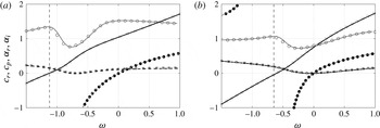
Figure 11. Incompressible solutions of (2.4) (lines) compared with Fernandez-Feria & del Pino (Reference Fernandez-Feria and del Pino2002) (symbols) for (a)
 $Re=90$
,
$Re=90$
,
 $\unicode[STIX]{x1D716}=1$
,
$\unicode[STIX]{x1D716}=1$
,
 $m=-1$
and (b)
$m=-1$
and (b)
 $Re=100$
,
$Re=100$
,
 $\unicode[STIX]{x1D716}=2$
,
$\unicode[STIX]{x1D716}=2$
,
 $m=-1$
with the following shown: (——, ○)
$m=-1$
with the following shown: (——, ○)
 $c_{r}$
, (– – –, ●)
$c_{r}$
, (– – –, ●)
 $c_{p}$
, (——, ▫)
$c_{p}$
, (——, ▫)
 $\unicode[STIX]{x1D6FC}_{r}$
, (– – –, ▪)
$\unicode[STIX]{x1D6FC}_{r}$
, (– – –, ▪)
 $\unicode[STIX]{x1D6FC}_{i}$
. The vertical dashed lines are discontinuities in
$\unicode[STIX]{x1D6FC}_{i}$
. The vertical dashed lines are discontinuities in
 $c_{p}$
(see text).
$c_{p}$
(see text).
In conclusion, we have demonstrated the primary role of entropic energy fluctuations in the hydrodynamic stability of compressible swirling pipe flows, with the computed stability boundaries shown to be significantly different from other swirling flows.
Acknowledgements
We acknowledge contributions from A. Mishra, on initiating this work as part of a Masters dissertation at IISc, and M. Barbate for help with the linear stability code. Partial funding from the National Centre for Combustion Research and Development (NCCRD) project via SERB sanction order number IR/S3/EU-01/2009, dated November 29th, 2011, is gratefully acknowledged.
Appendix A. Validation of the linear stability solver
Our first validation check is carried out against the non-swirling, incompressible Hagen–Poiseuille pipe flow results of Garg & Rouleau (Reference Garg and Rouleau1972) and Khorrami et al. (Reference Khorrami, Malik and Ash1989) at
 $Ma=0.01$
and
$Ma=0.01$
and
 $Re=10\,000$
for the
$Re=10\,000$
for the
 $\unicode[STIX]{x1D714}=0.5$
perturbations. The respective complex spatial growth rates for the least stable
$\unicode[STIX]{x1D714}=0.5$
perturbations. The respective complex spatial growth rates for the least stable
 $m=0$
and
$m=0$
and
 $m=1$
modes are shown in table 4 up to eleven decimal places along with computed values using the present solver. The eigenvalues of Garg & Rouleau (Reference Garg and Rouleau1972) are reported to be accurate to at least nine significant digits, whereas our computations show perfect match up to ten decimal places for
$m=1$
modes are shown in table 4 up to eleven decimal places along with computed values using the present solver. The eigenvalues of Garg & Rouleau (Reference Garg and Rouleau1972) are reported to be accurate to at least nine significant digits, whereas our computations show perfect match up to ten decimal places for
 $m=0$
and nine decimal places for the
$m=0$
and nine decimal places for the
 $m=1$
mode. On comparing with results of Khorrami et al. (Reference Khorrami, Malik and Ash1989), who use a different numerical method (Chebyshev collocation, similar to § 2.4 of this work), this match is seen up to eleven decimal places for
$m=1$
mode. On comparing with results of Khorrami et al. (Reference Khorrami, Malik and Ash1989), who use a different numerical method (Chebyshev collocation, similar to § 2.4 of this work), this match is seen up to eleven decimal places for
 $m=0$
and eight decimal places for
$m=0$
and eight decimal places for
 $m=1$
. In fact, Khorrami et al. (Reference Khorrami, Malik and Ash1989) report data only up to eight decimal places for
$m=1$
. In fact, Khorrami et al. (Reference Khorrami, Malik and Ash1989) report data only up to eight decimal places for
 $m=1$
and comment on a loss in accuracy of Garg & Rouleau (Reference Garg and Rouleau1972) beyond this, while our calculations show the latter to be correct up to nine decimal places, even for the
$m=1$
and comment on a loss in accuracy of Garg & Rouleau (Reference Garg and Rouleau1972) beyond this, while our calculations show the latter to be correct up to nine decimal places, even for the
 $m=1$
mode.
$m=1$
mode.
Next, we compare with two incompressible swirling pipe flow cases of Fernandez-Feria & del Pino (Reference Fernandez-Feria and del Pino2002), shown in figure 11 for the least stable (or most unstable) mode at the particular frequency
 $\unicode[STIX]{x1D714}$
. The real group velocities
$\unicode[STIX]{x1D714}$
. The real group velocities
 $c_{r}$
in both cases are always positive, indicating the direction of wavepacket propagation, as well as the direction of energy travel. The phase speeds
$c_{r}$
in both cases are always positive, indicating the direction of wavepacket propagation, as well as the direction of energy travel. The phase speeds
 $c_{p}$
can have either sign, and also have a discontinuity as
$c_{p}$
can have either sign, and also have a discontinuity as
 $\unicode[STIX]{x1D6FC}_{r}\rightarrow 0$
, shown by the vertical asymptotes in the figure. Both cases are barely unstable, with the lower-
$\unicode[STIX]{x1D6FC}_{r}\rightarrow 0$
, shown by the vertical asymptotes in the figure. Both cases are barely unstable, with the lower-
 $\unicode[STIX]{x1D716}$
case leading to instabilities at lower frequencies. The overall match obtained between our linear stability solver results and Fernandez-Feria & del Pino (Reference Fernandez-Feria and del Pino2002), as demonstrated in figure 11, is excellent.
$\unicode[STIX]{x1D716}$
case leading to instabilities at lower frequencies. The overall match obtained between our linear stability solver results and Fernandez-Feria & del Pino (Reference Fernandez-Feria and del Pino2002), as demonstrated in figure 11, is excellent.
Appendix B. Details of stability equation operators
Details of the operators
 $\unicode[STIX]{x1D647}_{i}$
of (2.4) are given in this appendix.
$\unicode[STIX]{x1D647}_{i}$
of (2.4) are given in this appendix.
 $$\begin{eqnarray}\displaystyle \unicode[STIX]{x1D647}_{1}=\left(\begin{array}{@{}ccccc@{}}\text{i}\left(m\bar{u}_{\unicode[STIX]{x1D703}}-\unicode[STIX]{x1D714}r\right) & r{\displaystyle \frac{\unicode[STIX]{x2202}\bar{\unicode[STIX]{x1D70C}}}{\unicode[STIX]{x2202}r}}+(r\text{D}+1)\bar{\unicode[STIX]{x1D70C}} & \text{i}m\bar{\unicode[STIX]{x1D70C}} & 0 & 0\\ -r\bar{u}_{\unicode[STIX]{x1D703}}^{2} & \text{i}r\bar{\unicode[STIX]{x1D70C}}(m\bar{u}_{\unicode[STIX]{x1D703}}-\unicode[STIX]{x1D714}r) & -2r\bar{\unicode[STIX]{x1D70C}}\bar{u}_{\unicode[STIX]{x1D703}} & 0 & r^{2}\text{D}\\ 0 & r\bar{\unicode[STIX]{x1D70C}}\left(\bar{u}_{\unicode[STIX]{x1D703}}+r{\displaystyle \frac{\unicode[STIX]{x2202}\bar{u}_{\unicode[STIX]{x1D703}}}{\unicode[STIX]{x2202}r}}\right) & \text{i}r\bar{\unicode[STIX]{x1D70C}}(m\bar{u}_{\unicode[STIX]{x1D703}}-\unicode[STIX]{x1D714}r) & 0 & \text{i}rm\\ 0 & r^{2}\bar{\unicode[STIX]{x1D70C}}{\displaystyle \frac{\unicode[STIX]{x2202}\bar{u}_{z}}{\unicode[STIX]{x2202}r}} & 0 & \text{i}r\bar{\unicode[STIX]{x1D70C}}(m\bar{u}_{\unicode[STIX]{x1D703}}-\unicode[STIX]{x1D714}r) & 0\\ -\text{i}(m\bar{u}_{\unicode[STIX]{x1D703}}-\unicode[STIX]{x1D714}r)\bar{T} & r\bar{\unicode[STIX]{x1D70C}}{\displaystyle \frac{\unicode[STIX]{x2202}\bar{T}}{\unicode[STIX]{x2202}r}}-(\unicode[STIX]{x1D6FE}-1)Ma^{2}r{\displaystyle \frac{\unicode[STIX]{x2202}\bar{p}}{\unicode[STIX]{x2202}r}} & 0 & 0 & \text{i}Ma^{2}(m\bar{u}_{\unicode[STIX]{x1D703}}-\unicode[STIX]{x1D714}r)\end{array}\right) & & \displaystyle \nonumber\\ \displaystyle & & \displaystyle\end{eqnarray}$$
 $$\begin{eqnarray}\displaystyle \unicode[STIX]{x1D647}_{2}=\left(\begin{array}{@{}ccccc@{}}\text{i}r\bar{u}_{z} & 0 & 0 & \text{i}r\bar{\unicode[STIX]{x1D70C}} & 0\\ 0 & \text{i}r^{2}\bar{\unicode[STIX]{x1D70C}}\bar{u}_{z} & 0 & 0 & 0\\ 0 & 0 & \text{i}r^{2}\bar{\unicode[STIX]{x1D70C}}\bar{u}_{z} & 0 & 0\\ 0 & 0 & 0 & \text{i}r^{2}\bar{\unicode[STIX]{x1D70C}}\bar{u}_{z} & \text{i}r^{2}\\ -\text{i}r\bar{u}_{z}\bar{T} & 0 & 0 & 0 & \text{i}Ma^{2}r\bar{u}_{z}\end{array}\right) & & \displaystyle\end{eqnarray}$$
 $$\begin{eqnarray}\displaystyle \unicode[STIX]{x1D647}_{3}=\left(\begin{array}{@{}ccccc@{}}0 & 0 & 0 & 0 & 0\\ 0 & -{\displaystyle \frac{4r}{3}}(r\text{D}^{2}+\text{D})+m^{2}+{\displaystyle \frac{4}{3}} & {\displaystyle \frac{\text{i}m}{3}}(7-r\text{D}) & 0 & 0\\ 0 & -{\displaystyle \frac{\text{i}m}{3}}(7+r\text{D}) & -r(r\text{D}^{2}+\text{D})+{\displaystyle \frac{4m^{2}}{3}}+1 & 0 & 0\\ 0 & 0 & 0 & -r(r\text{D}^{2}+\text{D})+m^{2} & 0\\ \unicode[STIX]{x1D613}_{51} & -2\text{i}m(\unicode[STIX]{x1D6FE}-1)Ma^{2}L_{\unicode[STIX]{x1D703}} & -2(\unicode[STIX]{x1D6FE}-1)Ma^{2}(r\text{D}-1)L_{\unicode[STIX]{x1D703}} & -2(\unicode[STIX]{x1D6FE}-1)Ma^{2}r\text{D}{\displaystyle \frac{\unicode[STIX]{x2202}\bar{u}_{z}}{\unicode[STIX]{x2202}r}} & \unicode[STIX]{x1D613}_{55}\end{array}\right) & & \displaystyle \nonumber\\ \displaystyle & & \displaystyle\end{eqnarray}$$
 $$\begin{eqnarray}\displaystyle & \displaystyle \unicode[STIX]{x1D647}_{4}=\left(\begin{array}{@{}ccccc@{}}0 & 0 & 0 & 0 & 0\\ 0 & 0 & 0 & -{\displaystyle \frac{\text{i}}{3}}r^{2}\text{D} & 0\\ 0 & 0 & 0 & {\displaystyle \frac{m}{3}}r & 0\\ 0 & -{\displaystyle \frac{\text{i}}{3}}r(r\text{D}+1) & {\displaystyle \frac{m}{3}}r & 0 & 0\\ 0 & -2\text{i}r(\unicode[STIX]{x1D6FE}-1)Ma^{2}{\displaystyle \frac{\unicode[STIX]{x2202}\bar{u}_{z}}{\unicode[STIX]{x2202}r}} & 0 & 0 & 0\end{array}\right) & \displaystyle\end{eqnarray}$$
 $$\begin{eqnarray}\displaystyle & \displaystyle \unicode[STIX]{x1D647}_{5}=\left(\begin{array}{@{}ccccc@{}}0 & 0 & 0 & 0 & 0\\ 0 & r^{2} & 0 & 0 & 0\\ 0 & 0 & r^{2} & 0 & 0\\ 0 & 0 & 0 & {\displaystyle \frac{4}{3}}r^{2} & 0\\ -{\displaystyle \frac{1}{Pr}}{\displaystyle \frac{r\bar{T}}{\bar{\unicode[STIX]{x1D70C}}}} & 0 & 0 & 0 & {\displaystyle \frac{\unicode[STIX]{x1D6FE}Ma^{2}}{Pr}}{\displaystyle \frac{r}{\bar{\unicode[STIX]{x1D70C}}}}\end{array}\right), & \displaystyle\end{eqnarray}$$
where
 $\text{D}=\text{d}/\text{d}r$
,
$\text{D}=\text{d}/\text{d}r$
,
 $\text{D}^{2}=\text{d}^{2}/\text{d}r^{2}$
,
$\text{D}^{2}=\text{d}^{2}/\text{d}r^{2}$
,
 $L_{\unicode[STIX]{x1D703}}=(\unicode[STIX]{x2202}\bar{u}_{\unicode[STIX]{x1D703}}/\unicode[STIX]{x2202}r-\bar{u}_{\unicode[STIX]{x1D703}}/r)$
,
$L_{\unicode[STIX]{x1D703}}=(\unicode[STIX]{x2202}\bar{u}_{\unicode[STIX]{x1D703}}/\unicode[STIX]{x2202}r-\bar{u}_{\unicode[STIX]{x1D703}}/r)$
,
 $$\begin{eqnarray}\displaystyle \unicode[STIX]{x1D613}_{51}={\displaystyle \frac{1}{Pr}}\left[\left(r\text{D}^{2}+\text{D}-{\displaystyle \frac{m^{2}}{r}}\right){\displaystyle \frac{\bar{T}}{\bar{\unicode[STIX]{x1D70C}}}}+(2r\text{D}+1){\displaystyle \frac{\unicode[STIX]{x2202}(\bar{T}/\bar{\unicode[STIX]{x1D70C}})}{\unicode[STIX]{x2202}r}}+r{\displaystyle \frac{\unicode[STIX]{x2202}^{2}(\bar{T}/\bar{\unicode[STIX]{x1D70C}})}{\unicode[STIX]{x2202}r^{2}}}\right], & & \displaystyle\end{eqnarray}$$
and
 $$\begin{eqnarray}\displaystyle \unicode[STIX]{x1D613}_{55}=-{\displaystyle \frac{\unicode[STIX]{x1D6FE}Ma^{2}}{Pr}}{\displaystyle \frac{1}{\bar{\unicode[STIX]{x1D70C}}}}\left[\left(r\text{D}^{2}+\text{D}-{\displaystyle \frac{m^{2}}{r}}\right)-(2r\text{D}+1){\displaystyle \frac{1}{\bar{\unicode[STIX]{x1D70C}}}}{\displaystyle \frac{\unicode[STIX]{x2202}\bar{\unicode[STIX]{x1D70C}}}{\unicode[STIX]{x2202}r}}-{\displaystyle \frac{r}{\bar{\unicode[STIX]{x1D70C}}}}{\displaystyle \frac{\unicode[STIX]{x2202}^{2}\bar{\unicode[STIX]{x1D70C}}}{\unicode[STIX]{x2202}r^{2}}}+2{\displaystyle \frac{r}{\bar{\unicode[STIX]{x1D70C}}^{2}}}\left({\displaystyle \frac{\unicode[STIX]{x2202}\bar{\unicode[STIX]{x1D70C}}}{\unicode[STIX]{x2202}r}}\right)^{2}\right].\quad & & \displaystyle\end{eqnarray}$$


