


1 Introduction
Superhydrophobic coatings prevent the sticking of drops on surfaces, a property used in the design of self-cleaning materials (Blossey Reference Blossey2003) or of anti-icing aircraft lifting surfaces (Mishchenko et al. Reference Mishchenko, Hatton, Bahadur, Taylor, Krupenkin and Aizenberg2010). Different types of leaves (lotus, eucalyptus, tulipa, etc.) are covered by a non-wetting material with a hierarchical microstructure that repels water (Quéré Reference Quéré2005), influencing the pathogen dispersal in agriculture by rain drops (Gart et al. Reference Gart, Mates, Megaridis and Jung2015; Gilet & Bourouiba Reference Gilet and Bourouiba2015) and the delivery of sprayed pesticides (Bergeron et al. Reference Bergeron, Bonn, Martin and Vovelle2000). Indeed, when the velocities of rain drops falling on infected plant leaves exceed the threshold value for splashing, tiny droplets, which could act as carriers of pathogens, are ejected at a velocity much larger than that of impact. The disease propagates when the emitted micron-sized droplets, which can be transported far away from the impact point thanks to their high speed, are deposited onto non-contaminated leaves (Lejeune, Gilet & Bourouiba Reference Lejeune, Gilet and Bourouiba2018).
It is known that the splash threshold velocity for millimetric water droplets impacting a smooth dry substrate under normal atmospheric conditions is
 ${\sim}$
4 m s
${\sim}$
4 m s
 $^{-1}$
(Riboux & Gordillo Reference Riboux and Gordillo2014, Reference Riboux and Gordillo2017; de Goede et al.
Reference de Goede, Laan, de Bruin and Bonn2018). However, when the solid substrate is covered with a superhydrophobic material, the transition to splashing takes place at far smaller values of the impact velocity,
$^{-1}$
(Riboux & Gordillo Reference Riboux and Gordillo2014, Reference Riboux and Gordillo2017; de Goede et al.
Reference de Goede, Laan, de Bruin and Bonn2018). However, when the solid substrate is covered with a superhydrophobic material, the transition to splashing takes place at far smaller values of the impact velocity,
 ${\sim}$
1.5 m s
${\sim}$
1.5 m s
 $^{-1}$
(Kim et al.
Reference Kim, Lee, Kim and Kim2012; Lv et al.
Reference Lv, Hao, Zhang and He2016). The reasons for the differences observed in the splashing threshold velocity are still not well understood and the purpose of this contribution is to provide a self-consistent physical model aimed at predicting the critical velocity for splashing when the drop falls onto a superhydrophobic substrate.
$^{-1}$
(Kim et al.
Reference Kim, Lee, Kim and Kim2012; Lv et al.
Reference Lv, Hao, Zhang and He2016). The reasons for the differences observed in the splashing threshold velocity are still not well understood and the purpose of this contribution is to provide a self-consistent physical model aimed at predicting the critical velocity for splashing when the drop falls onto a superhydrophobic substrate.
The splash criterion in Riboux & Gordillo (Reference Riboux and Gordillo2014, Reference Riboux and Gordillo2017), which was deduced for the case of partially wetting smooth solid surfaces, expresses that a necessary condition for splashing is that the edge of the expanding liquid sheet needs to be separated from the wall first. Indeed, the edge of the lamella is displaced vertically because it experiences an aerodynamic lift force per unit length which mainly results from the gas lubrication overpressure in the wedge region located between the advancing lamella and the solid. Hence, a necessary condition for the drop to disintegrate into smaller parts under the circumstances studied in Riboux & Gordillo (Reference Riboux and Gordillo2014, Reference Riboux and Gordillo2017) is that the edge of the advancing lamella must dewet the substrate first. This condition, however, is not sufficient for splashing because it might be that the edge separates vertically from the wall at a distance smaller than the radial growth of the rim caused by capillary retraction; if that were the case, the edge would rewet the solid and splashing would be inhibited. The main difference between the physical situation studied in Riboux & Gordillo (Reference Riboux and Gordillo2014, Reference Riboux and Gordillo2017) and the one at hand is that, for the case of superhydrophobic coatings, the edge of the lamella is always separated from the substrate, as figure 1(a) shows. Hence, the criterion for splashing on superhydrophobic surfaces will notably differ from the cases considered in Riboux & Gordillo (Reference Riboux and Gordillo2014, Reference Riboux and Gordillo2017). Here, we will limit ourselves to considering the most usual case of water droplets impacting a superhydrophobic solid under normal atmospheric conditions.
As will be shown below, our model can also be used to predict the diameters and velocities of the droplets ejected when the impact velocity exceeds the critical velocity for splashing. The analysis is limited to the study of the cases in which the drop disintegrates while it is expanding radially outwards because it is only under these conditions that the small droplets ejected are fast enough to travel large distances from the impact point.
The paper is structured as follows: experiments are described and analysed in §§ 2 and 3 is dedicated to presenting the equations governing the flow and to comparing the model predictions with experimental measurements while the main findings are summarized in § 4.

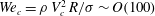
Figure 1. (a) High speed visualization of the spatial region connecting the lamella with the rim for several values of the Weber number (i)
 $We=60$
, (ii)
$We=60$
, (ii)
 $We=91$
, (iii)
$We=91$
, (iii)
 $We=140$
. These images show that, while the rim is never in contact with the substrate, the bottom part of the drop does touch the solid. (b) The measured ejection times corresponding to water droplets of different radii
$We=140$
. These images show that, while the rim is never in contact with the substrate, the bottom part of the drop does touch the solid. (b) The measured ejection times corresponding to water droplets of different radii
 $R$
impacting a superhydrophobic surface closely follow the prediction in Riboux & Gordillo (Reference Riboux and Gordillo2017),
$R$
impacting a superhydrophobic surface closely follow the prediction in Riboux & Gordillo (Reference Riboux and Gordillo2017),
 $t_{e}=1.05\,We^{-2/3}$
, since for all experimental conditions investigated here,
$t_{e}=1.05\,We^{-2/3}$
, since for all experimental conditions investigated here,
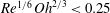 $Re^{1/6}\,Oh^{2/3}<0.25$
. The inset shows an instant close to that for which the lamella is ejected for the case of a droplet of radius
$Re^{1/6}\,Oh^{2/3}<0.25$
. The inset shows an instant close to that for which the lamella is ejected for the case of a droplet of radius
 $R=1.46$
mm and
$R=1.46$
mm and
 $We=317$
.
$We=317$
.
2 Experiments
Drops of different radii
 $R$
are generated quasi-statically at normal atmospheric conditions using hypodermic needles of different diameters placed at controllable height from the substrate; in this way, the droplets fall at different velocities
$R$
are generated quasi-statically at normal atmospheric conditions using hypodermic needles of different diameters placed at controllable height from the substrate; in this way, the droplets fall at different velocities
 $V$
onto a dry glass slide previously covered by Never Wet, a commercial superhydrophobic coating. The deposition of this type of superhydrophobic material over the glass slide forms a substrate with a hierarchical texture and random roughness which entraps air pockets (Lv et al.
Reference Lv, Hao, Zhang and He2016; Weisensee et al.
Reference Weisensee, Tian, Miljkovic and King2016). Notice that the type of superhydrophobic coating used here differs from the one used in similar contributions, where micro- or nanostructured materials were used (Tsai et al.
Reference Tsai, Hendrix, Dijkstra, Shui and Lohse2011). Both the chemical composition of the superhydrophobic material and the topology of the roughness favour the edge of the expanding lamella not being in contact with the substrate, as is visualized in figure 1(a), this being the reason behind the relatively small values for the critical Weber number for splashing with respect to the case of hydrophilic substrates (Riboux & Gordillo Reference Riboux and Gordillo2014, Reference Riboux and Gordillo2017), as will be shown below. However, it is also depicted in figure 1(a) that the bottom part of the droplet touches the substrate and, therefore, the liquid feeding the rim bordering the expanding liquid sheet is decelerated by the viscous shear stresses exerted at the wall. The experimental observation, to be shown below, that viscous shear contributes to decelerate the liquid flowing into the rim, even in the case of superhydrophobic substrates, contrasts with the ideas behind the model presented in Clanet et al. (Reference Clanet, Béguin, Richard and Quéré2004).
$V$
onto a dry glass slide previously covered by Never Wet, a commercial superhydrophobic coating. The deposition of this type of superhydrophobic material over the glass slide forms a substrate with a hierarchical texture and random roughness which entraps air pockets (Lv et al.
Reference Lv, Hao, Zhang and He2016; Weisensee et al.
Reference Weisensee, Tian, Miljkovic and King2016). Notice that the type of superhydrophobic coating used here differs from the one used in similar contributions, where micro- or nanostructured materials were used (Tsai et al.
Reference Tsai, Hendrix, Dijkstra, Shui and Lohse2011). Both the chemical composition of the superhydrophobic material and the topology of the roughness favour the edge of the expanding lamella not being in contact with the substrate, as is visualized in figure 1(a), this being the reason behind the relatively small values for the critical Weber number for splashing with respect to the case of hydrophilic substrates (Riboux & Gordillo Reference Riboux and Gordillo2014, Reference Riboux and Gordillo2017), as will be shown below. However, it is also depicted in figure 1(a) that the bottom part of the droplet touches the substrate and, therefore, the liquid feeding the rim bordering the expanding liquid sheet is decelerated by the viscous shear stresses exerted at the wall. The experimental observation, to be shown below, that viscous shear contributes to decelerate the liquid flowing into the rim, even in the case of superhydrophobic substrates, contrasts with the ideas behind the model presented in Clanet et al. (Reference Clanet, Béguin, Richard and Quéré2004).
Two high speed cameras with two different optical magnifications and acquisition rates have been used in our experimental study. The analysis of the videos recorded from the side at 340 000 frames per second (f.p.s.) with a spatial resolution of 10.5
 $\unicode[STIX]{x03BC}\text{m}~\text{pixel}^{-1}$
have allowed us to determine the instant at which the lamella is first ejected, see figure 1(b), whereas the experimental information needed to determine the radial position of the edge of the expanding liquid sheet – the rim – as well as the diameters and the velocities of the droplets ejected, are extracted from the videos recorded at 54 000 f.p.s. from the top (see figure 2), with a spatial resolution in this case of 16
$\unicode[STIX]{x03BC}\text{m}~\text{pixel}^{-1}$
have allowed us to determine the instant at which the lamella is first ejected, see figure 1(b), whereas the experimental information needed to determine the radial position of the edge of the expanding liquid sheet – the rim – as well as the diameters and the velocities of the droplets ejected, are extracted from the videos recorded at 54 000 f.p.s. from the top (see figure 2), with a spatial resolution in this case of 16
 $\unicode[STIX]{x03BC}\text{m}~\text{pixel}^{-1}$
. As was anticipated above, figure 2 shows that tiny droplets are emitted radially outwards for impact velocities above a threshold value which is below that found for the case of partially wetting substrates (Riboux & Gordillo Reference Riboux and Gordillo2014, Reference Riboux and Gordillo2017).
$\unicode[STIX]{x03BC}\text{m}~\text{pixel}^{-1}$
. As was anticipated above, figure 2 shows that tiny droplets are emitted radially outwards for impact velocities above a threshold value which is below that found for the case of partially wetting substrates (Riboux & Gordillo Reference Riboux and Gordillo2014, Reference Riboux and Gordillo2017).

Figure 2. Comparison between the predicted and the observed position of the rim bordering the expanding lamella for the case of a water droplet of radius
 $R=1.53$
mm impacting a superhydrophobic substrate. From left to right,
$R=1.53$
mm impacting a superhydrophobic substrate. From left to right,
 $V=1.67$
m s
$V=1.67$
m s
 $^{-1}$
(
$^{-1}$
(
 $We=60$
),
$We=60$
),
 $V=2.10$
m s
$V=2.10$
m s
 $^{-1}$
(
$^{-1}$
(
 $We=94$
) and
$We=94$
) and
 $V=3.16$
m s
$V=3.16$
m s
 $^{-1}$
(
$^{-1}$
(
 $We=214$
). The values of the dimensionless times corresponding to each line are: (a)
$We=214$
). The values of the dimensionless times corresponding to each line are: (a)
 $t=T\,(V/R)\approx 0$
, (b)
$t=T\,(V/R)\approx 0$
, (b)
 $t\approx 1.0$
, (c) 1.5, (d) 2.0 and (e) 3.0. Dashed yellow lines represent the numerical solution of the system (3.1), (3.3)–(3.5a,b
) while the continuous blue ones correspond to the solution of (3.1) using the analytical expressions for
$t\approx 1.0$
, (c) 1.5, (d) 2.0 and (e) 3.0. Dashed yellow lines represent the numerical solution of the system (3.1), (3.3)–(3.5a,b
) while the continuous blue ones correspond to the solution of (3.1) using the analytical expressions for
 $u$
and
$u$
and
 $h$
in (3.7). In both cases,
$h$
in (3.7). In both cases,
 $\unicode[STIX]{x1D706}=1$
.
$\unicode[STIX]{x1D706}=1$
.
From now on, both the experimental results and the equations describing the flow will be presented making use of the following dimensionless parameters:
 $Re=\unicode[STIX]{x1D70C}\,V\,R/\unicode[STIX]{x1D707}$
,
$Re=\unicode[STIX]{x1D70C}\,V\,R/\unicode[STIX]{x1D707}$
,
 $Oh=\unicode[STIX]{x1D707}/\sqrt{\unicode[STIX]{x1D70C}\,R\,\unicode[STIX]{x1D70E}}$
and
$Oh=\unicode[STIX]{x1D707}/\sqrt{\unicode[STIX]{x1D70C}\,R\,\unicode[STIX]{x1D70E}}$
and
 $We=Oh^{2}\,Re^{2}$
namely, the Reynolds, Ohnesorge and Weber numbers, with
$We=Oh^{2}\,Re^{2}$
namely, the Reynolds, Ohnesorge and Weber numbers, with
 $\unicode[STIX]{x1D70C}=1000$
kg m
$\unicode[STIX]{x1D70C}=1000$
kg m
 $^{-3}$
,
$^{-3}$
,
 $\unicode[STIX]{x1D707}=10^{-3}$
Pa s and
$\unicode[STIX]{x1D707}=10^{-3}$
Pa s and
 $\unicode[STIX]{x1D70E}=7.2\times 10^{-2}$
N m
$\unicode[STIX]{x1D70E}=7.2\times 10^{-2}$
N m
 $^{-1}$
denoting the water density, viscosity and interfacial tension coefficient, respectively. Dimensionless variables will be written using lower case letters to differentiate them from their dimensional counterparts (in capital letters) and distances, times and pressures will be made non-dimensional using, as characteristic values,
$^{-1}$
denoting the water density, viscosity and interfacial tension coefficient, respectively. Dimensionless variables will be written using lower case letters to differentiate them from their dimensional counterparts (in capital letters) and distances, times and pressures will be made non-dimensional using, as characteristic values,
 $R$
,
$R$
,
 $R/V$
and
$R/V$
and
 $\unicode[STIX]{x1D70C}V^{2}$
.
$\unicode[STIX]{x1D70C}V^{2}$
.
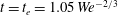
Setting the origin of time at the instant when the drop first touches the rough indentations located closer to the glass slide, the analysis of the experimental data shows that a thin lamella is first ejected from a radial position
 $r=\sqrt{3\,t_{e}}$
at a measured instant
$r=\sqrt{3\,t_{e}}$
at a measured instant
 $t_{e}$
which closely follows the theoretical predictions for the low Ohnesorge limit given in Riboux & Gordillo (Reference Riboux and Gordillo2014, Reference Riboux and Gordillo2017), namely,
$t_{e}$
which closely follows the theoretical predictions for the low Ohnesorge limit given in Riboux & Gordillo (Reference Riboux and Gordillo2014, Reference Riboux and Gordillo2017), namely,
 $t_{e}=1.05\,We^{-2/3}$
, see figure 1(b). The analysis of the images recorded from the top view, see figure 2, reveals that tiny droplets are expelled from the rim while it is expanding radially outwards only when the impact velocity exceeds a threshold value
$t_{e}=1.05\,We^{-2/3}$
, see figure 1(b). The analysis of the images recorded from the top view, see figure 2, reveals that tiny droplets are expelled from the rim while it is expanding radially outwards only when the impact velocity exceeds a threshold value
 $V_{c}\simeq 1.8$
m s
$V_{c}\simeq 1.8$
m s
 $^{-1}$
for water droplets of radii
$^{-1}$
for water droplets of radii
 $R\simeq 1.5\times 10^{-3}$
m. Figure 2 also shows that the speed of the droplets increases and their diameters decrease for increasing values of the impact velocity,
$R\simeq 1.5\times 10^{-3}$
m. Figure 2 also shows that the speed of the droplets increases and their diameters decrease for increasing values of the impact velocity,
 $V$
. Our purpose next will be to determine the dependence of
$V$
. Our purpose next will be to determine the dependence of
 $V_{c}$
on the control parameters and also to present a model which predicts the velocities and the diameters of the droplets issued from the rim as a function of
$V_{c}$
on the control parameters and also to present a model which predicts the velocities and the diameters of the droplets issued from the rim as a function of
 $We$
,
$We$
,
 $Oh$
and the dimensionless time after impact,
$Oh$
and the dimensionless time after impact,
 $t$
, for impact velocities above the splashing threshold.
$t$
, for impact velocities above the splashing threshold.

Figure 3. (a) Sketch showing the different variables used along the text. Here, (i) indicates the drop region,
 $0\leqslant r\leqslant \sqrt{3t}$
, (ii) indicates the lamella region,
$0\leqslant r\leqslant \sqrt{3t}$
, (ii) indicates the lamella region,
 $\sqrt{3t}\leqslant r\leqslant s(t)$
and (iii) the rim region; (b) representation using a spatio-temporal diagram of the different regions (i), (ii) and (iii) defined to analyse the flow.
$\sqrt{3t}\leqslant r\leqslant s(t)$
and (iii) the rim region; (b) representation using a spatio-temporal diagram of the different regions (i), (ii) and (iii) defined to analyse the flow.
3 Equations governing the flow and comparison with experiments
With the purpose of describing the dynamics of the rim limiting the expanding thin liquid sheet for times
 $t\geqslant t_{e}$
, it proves convenient to divide the flow into the three spatio-temporal regions illustrated in figure 3: (i) the drop region, which extends along the interval
$t\geqslant t_{e}$
, it proves convenient to divide the flow into the three spatio-temporal regions illustrated in figure 3: (i) the drop region, which extends along the interval
 $0\leqslant r\leqslant \sqrt{3t}$
, where pressure gradients cannot be neglected, (ii) the lamella, defined in the spatio-temporal region
$0\leqslant r\leqslant \sqrt{3t}$
, where pressure gradients cannot be neglected, (ii) the lamella, defined in the spatio-temporal region
 $\sqrt{3t}\leqslant r\leqslant s(t)$
and where pressure gradients can be safely neglected because the geometry of the thin liquid film is slender and (iii) a rim of thickness
$\sqrt{3t}\leqslant r\leqslant s(t)$
and where pressure gradients can be safely neglected because the geometry of the thin liquid film is slender and (iii) a rim of thickness
 $b(t)$
located at
$b(t)$
located at
 $r=s(t)$
(see figure 3). The lamella is thus a slender flow region extending from the end of the drop region,
$r=s(t)$
(see figure 3). The lamella is thus a slender flow region extending from the end of the drop region,
 $r=\sqrt{3t}$
, to the rim, located at
$r=\sqrt{3t}$
, to the rim, located at
 $r=s(t)$
.
$r=s(t)$
.
Both
 $s(t)$
and
$s(t)$
and
 $b(t)$
(see figure 3), can be calculated using the following mass and momentum balances (Taylor Reference Taylor1959; Culick Reference Culick1960),
$b(t)$
(see figure 3), can be calculated using the following mass and momentum balances (Taylor Reference Taylor1959; Culick Reference Culick1960),
 $$\begin{eqnarray}\displaystyle \left.\begin{array}{@{}l@{}}{\displaystyle \frac{\unicode[STIX]{x03C0}}{4}}{\displaystyle \frac{\text{d}b^{2}}{\text{d}t}}=[u(s,t)-v]h(s,t),\quad {\displaystyle \frac{\text{d}s}{\text{d}t}}=v,\\[12.0pt] {\displaystyle \frac{\unicode[STIX]{x03C0}\,b^{2}}{4}}{\displaystyle \frac{\text{d}v}{\text{d}t}}=[u(s,t)-v]^{2}\,h(s,t)-2\,We^{-1},\end{array}\right\} & & \displaystyle\end{eqnarray}$$
with
 $u(r,t)$
and
$u(r,t)$
and
 $h(r,t)$
in (3.1) the averaged velocity and the height of the liquid film in the region occupied by the lamella (
$h(r,t)$
in (3.1) the averaged velocity and the height of the liquid film in the region occupied by the lamella (
 $\sqrt{3t}\leqslant r\leqslant s(t)$
) (see figure 3
a). The equations for both
$\sqrt{3t}\leqslant r\leqslant s(t)$
) (see figure 3
a). The equations for both
 $u(r,t)$
and
$u(r,t)$
and
 $h(r,t)$
are deduced in Gordillo, Riboux & Quintero (Reference Gordillo, Riboux and Quintero2019) once the effect of the shear stress at the wall is added to the momentum equation using the results in Roisman (Reference Roisman2009), Eggers et al. (Reference Eggers, Fontelos, Josserand and Zaleski2010), where it is reported that the dimensionless boundary layer thickness only depends on time, and not on the distance to the axis of symmetry:
$h(r,t)$
are deduced in Gordillo, Riboux & Quintero (Reference Gordillo, Riboux and Quintero2019) once the effect of the shear stress at the wall is added to the momentum equation using the results in Roisman (Reference Roisman2009), Eggers et al. (Reference Eggers, Fontelos, Josserand and Zaleski2010), where it is reported that the dimensionless boundary layer thickness only depends on time, and not on the distance to the axis of symmetry:
 $\unicode[STIX]{x1D6FF}(t)=\sqrt{t/Re}$
. Therefore, the mass and momentum integral balances applied to a portion of the lamella of height
$\unicode[STIX]{x1D6FF}(t)=\sqrt{t/Re}$
. Therefore, the mass and momentum integral balances applied to a portion of the lamella of height
 $h$
, width
$h$
, width
 $\text{d}r$
and angular extension
$\text{d}r$
and angular extension
 $\text{d}\unicode[STIX]{x1D719}$
yield, respectively (Gordillo et al.
Reference Gordillo, Riboux and Quintero2019)
$\text{d}\unicode[STIX]{x1D719}$
yield, respectively (Gordillo et al.
Reference Gordillo, Riboux and Quintero2019)
 $$\begin{eqnarray}\displaystyle {\displaystyle \frac{\unicode[STIX]{x2202}(rh)}{\unicode[STIX]{x2202}\,t}}+{\displaystyle \frac{\unicode[STIX]{x2202}(ruh)}{\unicode[STIX]{x2202}\,r}}=0\quad \text{and}\quad {\displaystyle \frac{\unicode[STIX]{x2202}(ruh)}{\unicode[STIX]{x2202}\,t}}+{\displaystyle \frac{\unicode[STIX]{x2202}(ru^{2}h)}{\unicode[STIX]{x2202}\,r}}=-\unicode[STIX]{x1D706}{\displaystyle \frac{u\,r}{\sqrt{Re\,t}}}, & & \displaystyle\end{eqnarray}$$
with
 $\unicode[STIX]{x1D706}$
the friction factor which is adjusted experimentally because it absorbs the effects of the following assumptions in the model: (i) the velocity varies linearly within the boundary layer and (ii) the prefactor in the definition of the boundary layer thickness,
$\unicode[STIX]{x1D706}$
the friction factor which is adjusted experimentally because it absorbs the effects of the following assumptions in the model: (i) the velocity varies linearly within the boundary layer and (ii) the prefactor in the definition of the boundary layer thickness,
 $\unicode[STIX]{x1D6FF}(t)$
is fixed here to one i.e.
$\unicode[STIX]{x1D6FF}(t)$
is fixed here to one i.e.
 $\unicode[STIX]{x1D6FF}(t)=\sqrt{t/Re}$
. Moreover, the value of the friction factor
$\unicode[STIX]{x1D6FF}(t)=\sqrt{t/Re}$
. Moreover, the value of the friction factor
 $\unicode[STIX]{x1D706}$
will also take into account the deviations from the no-slip boundary condition at the wall, which is altered in the case of superhydrophobic substrates as a consequence of the entrapment of gas pockets in the corrugations of the solid.
$\unicode[STIX]{x1D706}$
will also take into account the deviations from the no-slip boundary condition at the wall, which is altered in the case of superhydrophobic substrates as a consequence of the entrapment of gas pockets in the corrugations of the solid.
Notice that both the momentum and continuity equation (3.2) can be written in a form appropriate to apply the method of characteristics along rays
 $\text{d}r/\text{d}t=u$
, see figure 3(b). Indeed, equation (3.2) can be alternatively written as
$\text{d}r/\text{d}t=u$
, see figure 3(b). Indeed, equation (3.2) can be alternatively written as
 $$\begin{eqnarray}\displaystyle {\displaystyle \frac{\unicode[STIX]{x2202}(rh)}{\unicode[STIX]{x2202}t}}+u{\displaystyle \frac{\unicode[STIX]{x2202}(rh)}{\unicode[STIX]{x2202}r}}=-rh{\displaystyle \frac{\unicode[STIX]{x2202}u}{\unicode[STIX]{x2202}r}}\;\Longrightarrow \;{\displaystyle \frac{\text{D}(rh)}{\text{D}t}}=-rh{\displaystyle \frac{\unicode[STIX]{x2202}u}{\unicode[STIX]{x2202}r}}\;\Longrightarrow \;{\displaystyle \frac{\text{D}\ln (rh)}{\text{D}t}}=-{\displaystyle \frac{\unicode[STIX]{x2202}u}{\unicode[STIX]{x2202}r}}, & & \displaystyle\end{eqnarray}$$
and
 $$\begin{eqnarray}\displaystyle {\displaystyle \frac{\unicode[STIX]{x2202}(ruh)}{\unicode[STIX]{x2202}\,t}}+{\displaystyle \frac{\unicode[STIX]{x2202}(ru^{2}h)}{\unicode[STIX]{x2202}\,r}} & \!=\! & \displaystyle u\left({\displaystyle \frac{\unicode[STIX]{x2202}(rh)}{\unicode[STIX]{x2202}\,t}}+{\displaystyle \frac{\unicode[STIX]{x2202}(ruh)}{\unicode[STIX]{x2202}\,r}}\right)+rh\left({\displaystyle \frac{\unicode[STIX]{x2202}\,u}{\unicode[STIX]{x2202}\,t}}+u{\displaystyle \frac{\unicode[STIX]{x2202}\,u}{\unicode[STIX]{x2202}\,r}}\right)=-\unicode[STIX]{x1D706}\frac{u\,r}{\sqrt{Re\,t}}\nonumber\\ \displaystyle & \!\;\Longrightarrow \;\! & \displaystyle \frac{\text{D}u}{\text{D}t}=-\unicode[STIX]{x1D706}\frac{u}{h\,\sqrt{Re\,t}},\end{eqnarray}$$
with
 $\text{D}/\text{D}t\equiv \unicode[STIX]{x2202}/\unicode[STIX]{x2202}\,t+u\,\unicode[STIX]{x2202}/\unicode[STIX]{x2202}r$
indicating the material derivative and where use of the continuity equation in (3.2) has been made.
$\text{D}/\text{D}t\equiv \unicode[STIX]{x2202}/\unicode[STIX]{x2202}\,t+u\,\unicode[STIX]{x2202}/\unicode[STIX]{x2202}r$
indicating the material derivative and where use of the continuity equation in (3.2) has been made.
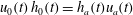
The fields
 $u(r,t)$
and
$u(r,t)$
and
 $h(r,t)$
are calculated in the spatio-temporal region
$h(r,t)$
are calculated in the spatio-temporal region
 $t\geqslant t_{e}$
,
$t\geqslant t_{e}$
,
 $\sqrt{3\,t}\leqslant r\leqslant s(t)$
using the method of characteristics once
$\sqrt{3\,t}\leqslant r\leqslant s(t)$
using the method of characteristics once
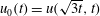 $u_{0}(t)=u(\sqrt{3t},t)$
and
$u_{0}(t)=u(\sqrt{3t},t)$
and
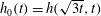 $h_{0}(t)=h(\sqrt{3t},t)$
are known at
$h_{0}(t)=h(\sqrt{3t},t)$
are known at
 $r=\sqrt{3t}$
from the solution of the flow in the drop region,
$r=\sqrt{3t}$
from the solution of the flow in the drop region,
 $0\leqslant r\leqslant \sqrt{3t}$
. In the free-slip limit,
$0\leqslant r\leqslant \sqrt{3t}$
. In the free-slip limit,
 $\unicode[STIX]{x1D706}=0$
,
$\unicode[STIX]{x1D706}=0$
,
 $u_{0}(t)$
and
$u_{0}(t)$
and
 $h_{0}(t)$
can be found numerically using a boundary element code since, in this case, the velocity field can be expressed as a function of a velocity potential, yielding
$h_{0}(t)$
can be found numerically using a boundary element code since, in this case, the velocity field can be expressed as a function of a velocity potential, yielding
 $u_{0}(t)=u_{a}(t)$
and
$u_{0}(t)=u_{a}(t)$
and
 $h_{0}(t)=h_{a}(t)$
with
$h_{0}(t)=h_{a}(t)$
with
 $u_{a}(t)=\sqrt{3/t}$
and
$u_{a}(t)=\sqrt{3/t}$
and
 $h_{a}(t)$
the functions given in Riboux & Gordillo (Reference Riboux and Gordillo2016), Gordillo et al. (Reference Gordillo, Riboux and Quintero2019) which are valid for all values of
$h_{a}(t)$
the functions given in Riboux & Gordillo (Reference Riboux and Gordillo2016), Gordillo et al. (Reference Gordillo, Riboux and Quintero2019) which are valid for all values of
 $t$
.
$t$
.
For
 $\unicode[STIX]{x1D706}\neq 0$
, a boundary layer of uniform dimensionless thickness
$\unicode[STIX]{x1D706}\neq 0$
, a boundary layer of uniform dimensionless thickness
 $\unicode[STIX]{x1D6FF}(t)=\sqrt{t/Re}$
develops in the region occupied by the lamella
$\unicode[STIX]{x1D6FF}(t)=\sqrt{t/Re}$
develops in the region occupied by the lamella
 $\sqrt{3t}\leqslant r\leqslant s(t)$
(Roisman Reference Roisman2009; Eggers et al.
Reference Eggers, Fontelos, Josserand and Zaleski2010). In this case, using a boundary layer description of the flow,
$\sqrt{3t}\leqslant r\leqslant s(t)$
(Roisman Reference Roisman2009; Eggers et al.
Reference Eggers, Fontelos, Josserand and Zaleski2010). In this case, using a boundary layer description of the flow,
 $u_{0}(t)$
and
$u_{0}(t)$
and
 $h_{0}(t)$
can be expressed as a function of their free-slip counterparts,
$h_{0}(t)$
can be expressed as a function of their free-slip counterparts,
 $u_{a}(t)$
and
$u_{a}(t)$
and
 $h_{a}(t)$
. Indeed, the velocity field at the drop interface in the region
$h_{a}(t)$
. Indeed, the velocity field at the drop interface in the region
 $0\leqslant r\leqslant \sqrt{3t}$
is not modified, in a first approximation, by the presence of the boundary layer. Therefore, for
$0\leqslant r\leqslant \sqrt{3t}$
is not modified, in a first approximation, by the presence of the boundary layer. Therefore, for
 $\unicode[STIX]{x1D706}\neq 0$
, the integral mass balance at the drop region indicates that flow rate entering into the lamella is the same as in the potential flow case,
$\unicode[STIX]{x1D706}\neq 0$
, the integral mass balance at the drop region indicates that flow rate entering into the lamella is the same as in the potential flow case,
 $\unicode[STIX]{x1D706}=0$
, a fact implying that, at
$\unicode[STIX]{x1D706}=0$
, a fact implying that, at
 $r=\sqrt{3t}$
,
$r=\sqrt{3t}$
,
 $u_{a}(t)\,h_{a}(t)=u_{a}(t)(h_{0}(t)-\unicode[STIX]{x1D6FF}(t))+u_{a}(t)\,\unicode[STIX]{x1D6FF}(t)/2$
. Here, we have used the approach in Gordillo et al. (Reference Gordillo, Riboux and Quintero2019) that the liquid velocity profile in the boundary layer varies linearly from zero at the wall to
$u_{a}(t)\,h_{a}(t)=u_{a}(t)(h_{0}(t)-\unicode[STIX]{x1D6FF}(t))+u_{a}(t)\,\unicode[STIX]{x1D6FF}(t)/2$
. Here, we have used the approach in Gordillo et al. (Reference Gordillo, Riboux and Quintero2019) that the liquid velocity profile in the boundary layer varies linearly from zero at the wall to
 $u_{a}(t)$
at a distance
$u_{a}(t)$
at a distance
 $\unicode[STIX]{x1D6FF}=\sqrt{t/Re}$
from the wall. Indeed, notice that the equations governing the time evolution of the rim thickness and velocity, given in (3.1), are not very sensitive to the specific velocity profile chosen to represent the boundary layer (see pages 319–320 in Batchelor (Reference Batchelor1967), where the integral method to analyse boundary layers firstly introduced by von Kármán is applied) because
$\unicode[STIX]{x1D6FF}=\sqrt{t/Re}$
from the wall. Indeed, notice that the equations governing the time evolution of the rim thickness and velocity, given in (3.1), are not very sensitive to the specific velocity profile chosen to represent the boundary layer (see pages 319–320 in Batchelor (Reference Batchelor1967), where the integral method to analyse boundary layers firstly introduced by von Kármán is applied) because
 $b(t)$
and
$b(t)$
and
 $s(t)$
depend on integral quantities i.e. the fluxes of mass and momentum. Hence, the partial differential equation (3.2) are deduced from local balances of mass and momentum with
$s(t)$
depend on integral quantities i.e. the fluxes of mass and momentum. Hence, the partial differential equation (3.2) are deduced from local balances of mass and momentum with
 $u$
representing the averaged value of the velocity in the direction perpendicular to the wall and then, from the definition of
$u$
representing the averaged value of the velocity in the direction perpendicular to the wall and then, from the definition of
 $u$
,
$u$
,
 $u_{0}(t)\,h_{0}(t)=h_{a}(t)u_{a}(t)$
, which together with the mass balance above involving
$u_{0}(t)\,h_{0}(t)=h_{a}(t)u_{a}(t)$
, which together with the mass balance above involving
 $\unicode[STIX]{x1D6FF}(t)$
yields (see Gordillo et al. (Reference Gordillo, Riboux and Quintero2019) for further details),
$\unicode[STIX]{x1D6FF}(t)$
yields (see Gordillo et al. (Reference Gordillo, Riboux and Quintero2019) for further details),
 $$\begin{eqnarray}\displaystyle h_{0}(t)=h_{a}(t)\left(1+{\displaystyle \frac{\unicode[STIX]{x1D6FF}(t)}{2\,h_{a}(t)}}\right),\quad u_{0}(t)=u_{a}(t)\left(1+{\displaystyle \frac{\unicode[STIX]{x1D6FF}(t)}{2\,h_{a}(t)}}\right)^{-1}\quad \text{with}~\unicode[STIX]{x1D6FF}(t)=\sqrt{t/Re}. & & \displaystyle \nonumber\\ \displaystyle & & \displaystyle\end{eqnarray}$$
The functions
 $u(r,t)$
and
$u(r,t)$
and
 $h(r,t)$
in (3.2), subjected to the boundary conditions (3.5), are calculated integrating in time equations (3.3)–(3.4) along rays
$h(r,t)$
in (3.2), subjected to the boundary conditions (3.5), are calculated integrating in time equations (3.3)–(3.4) along rays
 $\text{d}r/\text{d}t=u(r,t)$
departing from the spatio-temporal boundary
$\text{d}r/\text{d}t=u(r,t)$
departing from the spatio-temporal boundary
 $r=\sqrt{3x}$
with
$r=\sqrt{3x}$
with
 $x\geqslant t_{e}$
a parameter denoting time because
$x\geqslant t_{e}$
a parameter denoting time because
 $u_{0}(r=\sqrt{3x},x)$
and
$u_{0}(r=\sqrt{3x},x)$
and
 $h_{0}(\sqrt{3x},x)$
, are now known at the boundary separating the drop and lamella regions through (3.5). The integration in time is carried out using the characteristic form of the continuity and momentum equations given in (3.3)–(3.4) by means of a first-order Euler method. Indeed, given the values of
$h_{0}(\sqrt{3x},x)$
, are now known at the boundary separating the drop and lamella regions through (3.5). The integration in time is carried out using the characteristic form of the continuity and momentum equations given in (3.3)–(3.4) by means of a first-order Euler method. Indeed, given the values of
 $u(r,t)$
and
$u(r,t)$
and
 $h(r,t)$
at a fixed instant of time
$h(r,t)$
at a fixed instant of time
 $t>t_{e}$
, with
$t>t_{e}$
, with
 $r$
included in the spatio-temporal region
$r$
included in the spatio-temporal region
 $\sqrt{3t}\leqslant r\leqslant s(t)$
, the values of
$\sqrt{3t}\leqslant r\leqslant s(t)$
, the values of
 $u$
and
$u$
and
 $h$
at
$h$
at
 $t+\text{d}t$
are calculated at the new radial position
$t+\text{d}t$
are calculated at the new radial position
 $r+\text{d}r$
, with
$r+\text{d}r$
, with
 $\text{d}r=u(r,t)\text{d}t$
, once
$\text{d}r=u(r,t)\text{d}t$
, once
 $-\unicode[STIX]{x2202}\,u/\unicode[STIX]{x2202}r$
is determined at the instant
$-\unicode[STIX]{x2202}\,u/\unicode[STIX]{x2202}r$
is determined at the instant
 $t$
using a first-order backward finite difference scheme in space. Next, the value of the velocity is updated as
$t$
using a first-order backward finite difference scheme in space. Next, the value of the velocity is updated as
 $u(r+\text{d}r,t+\text{d}t)=u(r,t)+\text{d}u$
, with
$u(r+\text{d}r,t+\text{d}t)=u(r,t)+\text{d}u$
, with
 $\text{d}u=-\unicode[STIX]{x1D706}\,u(r,t)/(h(r,t)\sqrt{Re\,t})\,\text{d}t$
and
$\text{d}u=-\unicode[STIX]{x1D706}\,u(r,t)/(h(r,t)\sqrt{Re\,t})\,\text{d}t$
and
 $h(r+\text{d}r,t+\text{d}t)=h(r,t)+\text{d}h$
, with
$h(r+\text{d}r,t+\text{d}t)=h(r,t)+\text{d}h$
, with
 $\text{d}h$
calculated from
$\text{d}h$
calculated from
 $\text{d}[\ln (rh)]=-\unicode[STIX]{x2202}\,u/\unicode[STIX]{x2202}r\,\text{d}t$
, see (3.3)–(3.4).
$\text{d}[\ln (rh)]=-\unicode[STIX]{x2202}\,u/\unicode[STIX]{x2202}r\,\text{d}t$
, see (3.3)–(3.4).
Once
 $u(r,h)$
and
$u(r,h)$
and
 $h(r,t)$
are known within the spatio-temporal region
$h(r,t)$
are known within the spatio-temporal region
 $\sqrt{3t}\leqslant r\leqslant s(t)$
, the rim radial position and rim thickness,
$\sqrt{3t}\leqslant r\leqslant s(t)$
, the rim radial position and rim thickness,
 $s(t)$
and
$s(t)$
and
 $b(t)$
, are calculated integrating the ordinary differential equations in (3.1) once the functions
$b(t)$
, are calculated integrating the ordinary differential equations in (3.1) once the functions
 $u(r,t)$
and
$u(r,t)$
and
 $h(r,t)$
are particularized at
$h(r,t)$
are particularized at
 $r=s(t)$
and the following initial conditions are imposed at
$r=s(t)$
and the following initial conditions are imposed at
 $t=t_{e}=1.05\,We^{-2/3}$
(see Riboux & Gordillo (Reference Riboux and Gordillo2015) for details):
$t=t_{e}=1.05\,We^{-2/3}$
(see Riboux & Gordillo (Reference Riboux and Gordillo2015) for details):
 $$\begin{eqnarray}\displaystyle s(t_{e})=\sqrt{3\,t_{e}},\quad v(t_{e})=(1/2)\sqrt{3/t_{e}}\quad \text{and}\quad b(t_{e})=\sqrt{12}\,t_{e}^{3/2}/\unicode[STIX]{x03C0}. & & \displaystyle\end{eqnarray}$$
The good agreement depicted in figure 2 between experimental measurements and the time evolution of
 $s(t)$
predicted integrating equations (3.1) once the system (3.3)–(3.4) and (3.5) is solved using the numerical method described above, reveals that the model developed here correctly captures the effect of the viscous boundary layer on the drop spreading dynamics. But the time evolution of the spreading radius can be predicted in a much simpler way, avoiding the numerical integration of the system (3.3)–(3.4) and (3.5). Indeed, it was demonstrated in Gordillo et al. (Reference Gordillo, Riboux and Quintero2019) that the averaged velocity field and the height of the lamella,
$s(t)$
predicted integrating equations (3.1) once the system (3.3)–(3.4) and (3.5) is solved using the numerical method described above, reveals that the model developed here correctly captures the effect of the viscous boundary layer on the drop spreading dynamics. But the time evolution of the spreading radius can be predicted in a much simpler way, avoiding the numerical integration of the system (3.3)–(3.4) and (3.5). Indeed, it was demonstrated in Gordillo et al. (Reference Gordillo, Riboux and Quintero2019) that the averaged velocity field and the height of the lamella,
 $u(r,t)$
and
$u(r,t)$
and
 $h(r,t)$
, can be expressed, with errors
$h(r,t)$
, can be expressed, with errors
 ${\sim}O(Re^{-1})$
, as
${\sim}O(Re^{-1})$
, as
 $$\begin{eqnarray}\displaystyle \left\{\begin{array}{@{}l@{}}u(r,t)={\displaystyle \frac{r}{t}}-{\displaystyle \frac{Re^{-1/2}}{t}}\left[{\displaystyle \frac{\sqrt{3}\,\unicode[STIX]{x1D712}\,x}{2\,h_{a}(x)}}+{\displaystyle \frac{2\sqrt{3}\unicode[STIX]{x1D706}}{7h_{a}(x)x^{5/2}}}(t^{7/2}-x^{7/2})\right]+O(Re^{-1}),\\[12.0pt] h(r,t)=9{\displaystyle \frac{t^{2}}{r^{4}}}h_{a}[3(t/r)^{2}]+{\displaystyle \frac{Re^{-1/2}}{rt}}\left[{\displaystyle \frac{\sqrt{3}}{2}}x^{2}+{\displaystyle \frac{\sqrt{3}(105\,\unicode[STIX]{x1D712}-60\unicode[STIX]{x1D706})}{42}}x^{3}(t^{-1}-x^{-1})\right.\\[12.0pt] \left.\qquad \qquad +\,{\displaystyle \frac{24\sqrt{3}\unicode[STIX]{x1D706}}{105}}x^{-1/2}(t^{5/2}-x^{5/2})\right]+O(Re^{-1}),\end{array}\right. & & \displaystyle\end{eqnarray}$$
with
 $x=3(t/r)^{2}$
and
$x=3(t/r)^{2}$
and
 $\unicode[STIX]{x1D712}$
a constant such that
$\unicode[STIX]{x1D712}$
a constant such that
 $u_{0}(t)\simeq u_{a}(t)(1-\unicode[STIX]{x1D6FF}(t)\unicode[STIX]{x1D712}/(2\,h_{a}(t)))$
is a good approximation to the exact value in (3.5) for all values of
$u_{0}(t)\simeq u_{a}(t)(1-\unicode[STIX]{x1D6FF}(t)\unicode[STIX]{x1D712}/(2\,h_{a}(t)))$
is a good approximation to the exact value in (3.5) for all values of
 $t$
. Indeed, for
$t$
. Indeed, for
 $\unicode[STIX]{x1D6FF}/h_{a}\ll 1$
, the Taylor expansion of the equation for
$\unicode[STIX]{x1D6FF}/h_{a}\ll 1$
, the Taylor expansion of the equation for
 $u_{0}$
in (3.5) indicates that
$u_{0}$
in (3.5) indicates that
 $\unicode[STIX]{x1D712}=1$
but, for instance, consider that
$\unicode[STIX]{x1D712}=1$
but, for instance, consider that
 $\unicode[STIX]{x1D6FF}/h\simeq 1$
: in this case,
$\unicode[STIX]{x1D6FF}/h\simeq 1$
: in this case,
 $u_{0}(t)\simeq u_{a}(t)(1-\unicode[STIX]{x1D6FF}(t)\unicode[STIX]{x1D712}/(2\,h_{a}(t)))$
would be, for
$u_{0}(t)\simeq u_{a}(t)(1-\unicode[STIX]{x1D6FF}(t)\unicode[STIX]{x1D712}/(2\,h_{a}(t)))$
would be, for
 $\unicode[STIX]{x1D712}=2/3$
, an excellent approximation to the initial condition in (3.5). For the range of Ohnesorge numbers considered here,
$\unicode[STIX]{x1D712}=2/3$
, an excellent approximation to the initial condition in (3.5). For the range of Ohnesorge numbers considered here,
 $10^{-3}\lesssim Oh\lesssim 10^{-2}$
, the ratio
$10^{-3}\lesssim Oh\lesssim 10^{-2}$
, the ratio
 $\unicode[STIX]{x1D6FF}(t)/h_{a}(t)\sim 1$
and then, the linearized expression
$\unicode[STIX]{x1D6FF}(t)/h_{a}(t)\sim 1$
and then, the linearized expression
 $u_{0}(t)\simeq u_{a}(t)(1-\unicode[STIX]{x1D6FF}(t)\unicode[STIX]{x1D712}/(2\,h_{a}(t)))$
is a very good approximation to the exact value of
$u_{0}(t)\simeq u_{a}(t)(1-\unicode[STIX]{x1D6FF}(t)\unicode[STIX]{x1D712}/(2\,h_{a}(t)))$
is a very good approximation to the exact value of
 $u_{0}$
given in (3.5) for
$u_{0}$
given in (3.5) for
 $\unicode[STIX]{x1D712}=0.6$
, see figure 4. Based on this fact, all the results presented here have been calculated for
$\unicode[STIX]{x1D712}=0.6$
, see figure 4. Based on this fact, all the results presented here have been calculated for
 $\unicode[STIX]{x1D712}=0.6$
. Notice, however, that for values of the Ohnesorge number larger than those considered in this study, the ratio
$\unicode[STIX]{x1D712}=0.6$
. Notice, however, that for values of the Ohnesorge number larger than those considered in this study, the ratio
 $\unicode[STIX]{x1D6FF}(t)/h_{a}(t)$
could be
$\unicode[STIX]{x1D6FF}(t)/h_{a}(t)$
could be
 $\unicode[STIX]{x1D6FF}(t)/h_{a}(t)>1$
and then, the value of
$\unicode[STIX]{x1D6FF}(t)/h_{a}(t)>1$
and then, the value of
 $\unicode[STIX]{x1D712}$
in (3.7) would then be even smaller i.e.
$\unicode[STIX]{x1D712}$
in (3.7) would then be even smaller i.e.
 $\unicode[STIX]{x1D712}<0.6$
.
$\unicode[STIX]{x1D712}<0.6$
.

Figure 4. (a) Time evolution of the function
 $h_{a}(t)$
given in Riboux & Gordillo (Reference Riboux and Gordillo2016), Gordillo et al. (Reference Gordillo, Riboux and Quintero2019) and
$h_{a}(t)$
given in Riboux & Gordillo (Reference Riboux and Gordillo2016), Gordillo et al. (Reference Gordillo, Riboux and Quintero2019) and
 $h_{0}(r=\sqrt{3t},t)$
defined in (3.5). The inset shows that the ratio
$h_{0}(r=\sqrt{3t},t)$
defined in (3.5). The inset shows that the ratio
 $\unicode[STIX]{x1D6FF}(t)/h_{a}(t)$
is of order unity. (b) Time evolution of
$\unicode[STIX]{x1D6FF}(t)/h_{a}(t)$
is of order unity. (b) Time evolution of
 $u_{a}(t)=\sqrt{3/t}$
,
$u_{a}(t)=\sqrt{3/t}$
,
 $u_{0}(t)$
defined in (3.5) and the approximation
$u_{0}(t)$
defined in (3.5) and the approximation
 $u_{0}(t)\simeq u_{a}(t)(1-\unicode[STIX]{x1D6FF}(t)\unicode[STIX]{x1D712}/(2\,h_{a}(t)))$
with
$u_{0}(t)\simeq u_{a}(t)(1-\unicode[STIX]{x1D6FF}(t)\unicode[STIX]{x1D712}/(2\,h_{a}(t)))$
with
 $\unicode[STIX]{x1D712}=0.6$
. Here,
$\unicode[STIX]{x1D712}=0.6$
. Here,
 $We=100$
and
$We=100$
and
 $Oh=2.9\times 10^{-3}$
.
$Oh=2.9\times 10^{-3}$
.

Figure 5. Effect of varying the value of the friction factor
 $\unicode[STIX]{x1D706}$
in (3.7). (a)
$\unicode[STIX]{x1D706}$
in (3.7). (a)
 $t=T(R/V)\simeq 0$
, (b) 0.4, (c) 0.7, (d) 0.9, (e) 1.2, (f) 1.4, (g) 1.9, (h) 2.4, (i) 2.9. The continuous lines represent the solution of the ordinary differential equations in (3.1) using the analytical expressions of
$t=T(R/V)\simeq 0$
, (b) 0.4, (c) 0.7, (d) 0.9, (e) 1.2, (f) 1.4, (g) 1.9, (h) 2.4, (i) 2.9. The continuous lines represent the solution of the ordinary differential equations in (3.1) using the analytical expressions of
 $u$
and
$u$
and
 $h$
in (3.7) for:
$h$
in (3.7) for:
 $Re\rightarrow \infty$
, namely, free-slip case (black),
$Re\rightarrow \infty$
, namely, free-slip case (black),
 $\unicode[STIX]{x1D706}=0.5$
(green),
$\unicode[STIX]{x1D706}=0.5$
(green),
 $\unicode[STIX]{x1D706}=1$
(blue),
$\unicode[STIX]{x1D706}=1$
(blue),
 $\unicode[STIX]{x1D706}=2$
(red).
$\unicode[STIX]{x1D706}=2$
(red).
The integration of the ordinary differential equations in (3.1) using the analytical expressions for
 $u$
and
$u$
and
 $h$
in (3.7) particularized at
$h$
in (3.7) particularized at
 $r=s(t)$
, also represented in figure 2, reveals that the results obtained in this way are indistinguishable from those calculated solving numerically the system (3.3)–(3.4) and (3.5). Therefore, from now on, the results presented will be calculated using the analytical expressions for
$r=s(t)$
, also represented in figure 2, reveals that the results obtained in this way are indistinguishable from those calculated solving numerically the system (3.3)–(3.4) and (3.5). Therefore, from now on, the results presented will be calculated using the analytical expressions for
 $u$
and
$u$
and
 $h$
given in (3.7).
$h$
given in (3.7).
The sensitivity analysis to variations of
 $\unicode[STIX]{x1D706}$
is analysed in figure 5, where the spreading radius predicted by solving the system of (3.1) using the analytical values of
$\unicode[STIX]{x1D706}$
is analysed in figure 5, where the spreading radius predicted by solving the system of (3.1) using the analytical values of
 $u$
and
$u$
and
 $h$
given in (3.7), is shown for different cases and different instants of time. For instance, the predicted spreading radius
$h$
given in (3.7), is shown for different cases and different instants of time. For instance, the predicted spreading radius
 $s(t)$
in the limit
$s(t)$
in the limit
 $Re\rightarrow \infty$
, which corresponds to droplets in the Leidenfrost regime i.e. to the purely free-slip case, is much larger than the one observed experimentally, a fact revealing that viscous friction plays a major role in the spreading of droplets impacting a superhydrophobic substrate. Figure 5 also shows that, as expected, the calculated radii increase for decreasing values of
$Re\rightarrow \infty$
, which corresponds to droplets in the Leidenfrost regime i.e. to the purely free-slip case, is much larger than the one observed experimentally, a fact revealing that viscous friction plays a major role in the spreading of droplets impacting a superhydrophobic substrate. Figure 5 also shows that, as expected, the calculated radii increase for decreasing values of
 $\unicode[STIX]{x1D706}$
i.e. for decreasing values of the shear stress at the wall. Notice that one of the effects of increasing the proportion of gas pockets beneath the drop would be to decrease the value of the friction factor
$\unicode[STIX]{x1D706}$
i.e. for decreasing values of the shear stress at the wall. Notice that one of the effects of increasing the proportion of gas pockets beneath the drop would be to decrease the value of the friction factor
 $\unicode[STIX]{x1D706}$
. Although the differences observed in figure 5 for different values of
$\unicode[STIX]{x1D706}$
. Although the differences observed in figure 5 for different values of
 $\unicode[STIX]{x1D706}$
are not large, the best agreement between predictions and the experiments carried out here using superhydrophobic substrates with a hierarchical texture and random roughness is achieved for
$\unicode[STIX]{x1D706}$
are not large, the best agreement between predictions and the experiments carried out here using superhydrophobic substrates with a hierarchical texture and random roughness is achieved for
 $\unicode[STIX]{x1D706}=1$
, a value which coincides with that found in Gordillo et al. (Reference Gordillo, Riboux and Quintero2019). The results presented from now on will correspond to
$\unicode[STIX]{x1D706}=1$
, a value which coincides with that found in Gordillo et al. (Reference Gordillo, Riboux and Quintero2019). The results presented from now on will correspond to
 $\unicode[STIX]{x1D706}=1$
, but this choice made here does not imply that exactly the same value of
$\unicode[STIX]{x1D706}=1$
, but this choice made here does not imply that exactly the same value of
 $\unicode[STIX]{x1D706}$
should be used to describe the spreading and splashing of droplets impacting other types of superhydrophobic substrates. Indeed,
$\unicode[STIX]{x1D706}$
should be used to describe the spreading and splashing of droplets impacting other types of superhydrophobic substrates. Indeed,
 $\unicode[STIX]{x1D706}$
is the friction factor and hence, its value is influenced by the amount of gas entrapped beneath the drop, which depends on how the solid substrate is micro- or nanostructured.
$\unicode[STIX]{x1D706}$
is the friction factor and hence, its value is influenced by the amount of gas entrapped beneath the drop, which depends on how the solid substrate is micro- or nanostructured.

Figure 6. (a) Comparison between the predicted and the measured position of the rim bordering the expanding lamella for several values of
 $We$
. The inset sketches that the experimental value of
$We$
. The inset sketches that the experimental value of
 $s(t)$
corresponding to the averaged measurement of the radial position of the outer edge of the rim at two different angles for which no corrugations are developed. In (b), the values of the maximum spreading radius measured here (blue circles) together with the data in [1] Clanet et al. (Reference Clanet, Béguin, Richard and Quéré2004), [2] Tsai et al. (Reference Tsai, Hendrix, Dijkstra, Shui and Lohse2011), [3] Antonini, Amirfazli & Marengo (Reference Antonini, Amirfazli and Marengo2012) are compared with the values predicted by the model (black continuous line,
$s(t)$
corresponding to the averaged measurement of the radial position of the outer edge of the rim at two different angles for which no corrugations are developed. In (b), the values of the maximum spreading radius measured here (blue circles) together with the data in [1] Clanet et al. (Reference Clanet, Béguin, Richard and Quéré2004), [2] Tsai et al. (Reference Tsai, Hendrix, Dijkstra, Shui and Lohse2011), [3] Antonini, Amirfazli & Marengo (Reference Antonini, Amirfazli and Marengo2012) are compared with the values predicted by the model (black continuous line,
 $\unicode[STIX]{x1D706}=1$
); the Weber number defined here is based on the drop radius, whereas in Clanet et al. (Reference Clanet, Béguin, Richard and Quéré2004), Antonini et al. (Reference Antonini, Amirfazli and Marengo2012) the Weber number is defined using the diameter; also in (b), the experimental values in [4] Tran et al. (Reference Tran, Staat, Prosperetti, Sun and Lohse2012) are compared with those predicted for the case
$\unicode[STIX]{x1D706}=1$
); the Weber number defined here is based on the drop radius, whereas in Clanet et al. (Reference Clanet, Béguin, Richard and Quéré2004), Antonini et al. (Reference Antonini, Amirfazli and Marengo2012) the Weber number is defined using the diameter; also in (b), the experimental values in [4] Tran et al. (Reference Tran, Staat, Prosperetti, Sun and Lohse2012) are compared with those predicted for the case
 $Re\rightarrow \infty$
(thick red dashed line). The dashed thin black line represents the maximum spreading radius predicted by the theory in [5] Wildeman et al. (Reference Wildeman, Visser, Sun and Lohse2016), based on energetic arguments.
$Re\rightarrow \infty$
(thick red dashed line). The dashed thin black line represents the maximum spreading radius predicted by the theory in [5] Wildeman et al. (Reference Wildeman, Visser, Sun and Lohse2016), based on energetic arguments.
Figure 6(a) shows that the solution of (3.1) subjected to the initial conditions in (3.6) with
 $t=t_{e}=1.05\,We^{-2/3}$
and
$t=t_{e}=1.05\,We^{-2/3}$
and
 $u$
and
$u$
and
 $h$
given in (3.7), reproduces the time evolution of the drop spreading radius determined experimentally. Notice that the experimental measurements shown in this figure (with errors of the order of the image resolution, 16
$h$
given in (3.7), reproduces the time evolution of the drop spreading radius determined experimentally. Notice that the experimental measurements shown in this figure (with errors of the order of the image resolution, 16
 $\unicode[STIX]{x03BC}$
m pixel
$\unicode[STIX]{x03BC}$
m pixel
 $^{-1}$
, which cannot be appreciated in this plot) represent the averaged radial position of the edge of the rim i.e. of the outer contour of the rim, measured at two different angular directions at which it was checked that no capillary corrugations are observed for all values of
$^{-1}$
, which cannot be appreciated in this plot) represent the averaged radial position of the edge of the rim i.e. of the outer contour of the rim, measured at two different angular directions at which it was checked that no capillary corrugations are observed for all values of
 $t$
, see the sketch in the inset of figure 6(a). Moreover, figure 6(b), shows that our model is also able to predict the measured maximum spreading radius
$t$
, see the sketch in the inset of figure 6(a). Moreover, figure 6(b), shows that our model is also able to predict the measured maximum spreading radius
 $s_{max}$
in the free-slip limit,
$s_{max}$
in the free-slip limit,
 $Re\rightarrow \infty$
(Tran et al.
Reference Tran, Staat, Prosperetti, Sun and Lohse2012; Wildeman et al.
Reference Wildeman, Visser, Sun and Lohse2016). The predicted values of
$Re\rightarrow \infty$
(Tran et al.
Reference Tran, Staat, Prosperetti, Sun and Lohse2012; Wildeman et al.
Reference Wildeman, Visser, Sun and Lohse2016). The predicted values of
 $s_{max}$
for the case of superhydrophobic substrates,
$s_{max}$
for the case of superhydrophobic substrates,
 $\unicode[STIX]{x1D706}=1$
, are also in good agreement with our own experimental data and with the experiments available in the literature (Clanet et al.
Reference Clanet, Béguin, Richard and Quéré2004; Tsai et al.
Reference Tsai, Hendrix, Dijkstra, Shui and Lohse2011; Antonini et al.
Reference Antonini, Amirfazli and Marengo2012; Wildeman et al.
Reference Wildeman, Visser, Sun and Lohse2016).
$\unicode[STIX]{x1D706}=1$
, are also in good agreement with our own experimental data and with the experiments available in the literature (Clanet et al.
Reference Clanet, Béguin, Richard and Quéré2004; Tsai et al.
Reference Tsai, Hendrix, Dijkstra, Shui and Lohse2011; Antonini et al.
Reference Antonini, Amirfazli and Marengo2012; Wildeman et al.
Reference Wildeman, Visser, Sun and Lohse2016).

Figure 7. Time evolution of the ratio
 $t_{c}/t_{h}$
for different values of the Weber number and
$t_{c}/t_{h}$
for different values of the Weber number and
 $Oh=2.9\times 10^{-3}$
. The horizontal blue band indicates the critical value
$Oh=2.9\times 10^{-3}$
. The horizontal blue band indicates the critical value
 $0.1\pm 0.02$
, below which the capillary time
$0.1\pm 0.02$
, below which the capillary time
 $t_{c}$
is sufficiently small when compared with the hydrodynamic time
$t_{c}$
is sufficiently small when compared with the hydrodynamic time
 $t_{h}$
to produce the capillary breakup of the toroidal rim. The curve corresponding to
$t_{h}$
to produce the capillary breakup of the toroidal rim. The curve corresponding to
 $We=50$
never crosses the horizontal blue band, a fact indicating that the rim is stable to capillary perturbations. However, the curves corresponding to values of the Weber number
$We=50$
never crosses the horizontal blue band, a fact indicating that the rim is stable to capillary perturbations. However, the curves corresponding to values of the Weber number
 $We\gtrsim 70$
, cross the horizontal band at the breakup time
$We\gtrsim 70$
, cross the horizontal band at the breakup time
 $t_{b}$
, which decreases for increasing values of
$t_{b}$
, which decreases for increasing values of
 $We$
. The critical Weber number is calculated as the smaller value of
$We$
. The critical Weber number is calculated as the smaller value of
 $We$
for which
$We$
for which
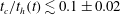 $t_{c}/t_{h}(t)\lesssim 0.1\pm 0.02$
for at least one value of
$t_{c}/t_{h}(t)\lesssim 0.1\pm 0.02$
for at least one value of
 $t$
.
$t$
.

Figure 8. The calculated values of the critical Weber number for normal atmospheric conditions and different values of the Ohnesorge number. The black continuous line corresponds to the values of
 $We_{c}$
calculated using the theory in Riboux & Gordillo (Reference Riboux and Gordillo2014, Reference Riboux and Gordillo2017) [1], which is applicable to the cases of partially wetting smooth solid substrates and is in very good agreement with experiments. The red band represent the range of values of the critical Weber number calculated using the criterion
$We_{c}$
calculated using the theory in Riboux & Gordillo (Reference Riboux and Gordillo2014, Reference Riboux and Gordillo2017) [1], which is applicable to the cases of partially wetting smooth solid substrates and is in very good agreement with experiments. The red band represent the range of values of the critical Weber number calculated using the criterion
 $t_{c}/t_{h}\leqslant 0.1\pm 0.02$
with the values of
$t_{c}/t_{h}\leqslant 0.1\pm 0.02$
with the values of
 $u$
and
$u$
and
 $h$
given by (3.7) in the limit
$h$
given by (3.7) in the limit
 $Re\rightarrow \infty$
, corresponding to the impact of droplets in the Leidenfrost regime. The values obtained are in very good agreement with the results in Staat et al. (Reference Staat, Tran, Geerdink, Riboux, Sun, Gordillo and Lohse2015), Riboux & Gordillo (Reference Riboux and Gordillo2016). The blue band represent the values of the critical Weber number calculated using the criterion
$Re\rightarrow \infty$
, corresponding to the impact of droplets in the Leidenfrost regime. The values obtained are in very good agreement with the results in Staat et al. (Reference Staat, Tran, Geerdink, Riboux, Sun, Gordillo and Lohse2015), Riboux & Gordillo (Reference Riboux and Gordillo2016). The blue band represent the values of the critical Weber number calculated using the criterion
 $t_{c}/t_{h}\leqslant 0.1\pm 0.02$
with the values of
$t_{c}/t_{h}\leqslant 0.1\pm 0.02$
with the values of
 $u$
and
$u$
and
 $h$
given by (3.7) for the case of a superhydrophobic substrate,
$h$
given by (3.7) for the case of a superhydrophobic substrate,
 $\unicode[STIX]{x1D706}=1$
. The values obtained are in very good agreement with the experimental measurements (dots) for different values of
$\unicode[STIX]{x1D706}=1$
. The values obtained are in very good agreement with the experimental measurements (dots) for different values of
 $Oh$
.
$Oh$
.
Our theory can also be used to compute both the critical conditions for splashing as well as the instant of time
 $t_{b}$
at which the rim starts to disintegrate. Indeed,
$t_{b}$
at which the rim starts to disintegrate. Indeed,
 $t_{b}$
is calculated using the criterion developed in Riboux & Gordillo (Reference Riboux and Gordillo2015), which expresses that drops will only be ejected when the time characterizing the radial growth of the rim,
$t_{b}$
is calculated using the criterion developed in Riboux & Gordillo (Reference Riboux and Gordillo2015), which expresses that drops will only be ejected when the time characterizing the radial growth of the rim,
 $T_{h}=(R/V)t_{h}=(R/V)(1/b\,\text{d}b/\text{d}t)^{-1}$
, is substantially larger than the capillary time
$T_{h}=(R/V)t_{h}=(R/V)(1/b\,\text{d}b/\text{d}t)^{-1}$
, is substantially larger than the capillary time
 $T_{c}=(R/V)t_{c}=(\unicode[STIX]{x1D70C}\,R^{3}\,b^{3}/8\unicode[STIX]{x1D70E})^{1/2}$
. In Riboux & Gordillo (Reference Riboux and Gordillo2015), the instant at which droplets are ejected from the rim was determined based on the following facts: (i) the time characterizing the radial growth of a capillary instability is
$T_{c}=(R/V)t_{c}=(\unicode[STIX]{x1D70C}\,R^{3}\,b^{3}/8\unicode[STIX]{x1D70E})^{1/2}$
. In Riboux & Gordillo (Reference Riboux and Gordillo2015), the instant at which droplets are ejected from the rim was determined based on the following facts: (i) the time characterizing the radial growth of a capillary instability is
 ${\sim}3T_{c}$
(Eggers & Villermaux Reference Eggers and Villermaux2008), (ii) the classical Rayleigh stability analysis reveals that the wavenumber corresponding to the fastest capillary instability growing in a cylindrical jet is
${\sim}3T_{c}$
(Eggers & Villermaux Reference Eggers and Villermaux2008), (ii) the classical Rayleigh stability analysis reveals that the wavenumber corresponding to the fastest capillary instability growing in a cylindrical jet is
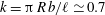 $k=\unicode[STIX]{x03C0}\,R\,b/\ell \simeq 0.7$
, with
$k=\unicode[STIX]{x03C0}\,R\,b/\ell \simeq 0.7$
, with
 $\ell$
the wavelength of the perturbation, which is assumed to be constant in time and (iii) for
$\ell$
the wavelength of the perturbation, which is assumed to be constant in time and (iii) for
 $k\geqslant 1$
, the growth of capillary instabilities is inhibited (Eggers & Villermaux Reference Eggers and Villermaux2008). Thus, for capillary corrugations with initial wavenumber
$k\geqslant 1$
, the growth of capillary instabilities is inhibited (Eggers & Villermaux Reference Eggers and Villermaux2008). Thus, for capillary corrugations with initial wavenumber
 $k=0.7$
to be amplified up to the point where the drops are ejected from the rim, it is necessary that in a time
$k=0.7$
to be amplified up to the point where the drops are ejected from the rim, it is necessary that in a time
 $3T_{c}$
,
$3T_{c}$
,
 $\unicode[STIX]{x0394}k<0.3$
, namely,
$\unicode[STIX]{x0394}k<0.3$
, namely,
 $(\text{d}b/\text{d}t)\times 3\,t_{c}\lesssim 0.3\,b\Rightarrow t_{c}/t_{h}\lesssim 0.1$
. Figure 7, which shows the time evolution of the ratio
$(\text{d}b/\text{d}t)\times 3\,t_{c}\lesssim 0.3\,b\Rightarrow t_{c}/t_{h}\lesssim 0.1$
. Figure 7, which shows the time evolution of the ratio
 $t_{c}/t_{h}$
as a function of time, reveals that capillary instabilities will only break the rim for values of the Weber number above a certain threshold,
$t_{c}/t_{h}$
as a function of time, reveals that capillary instabilities will only break the rim for values of the Weber number above a certain threshold,
 $We_{c}$
and also that the breakup time,
$We_{c}$
and also that the breakup time,
 $t_{b}$
, decreases for increasing values of
$t_{b}$
, decreases for increasing values of
 $We>We_{c}$
. Figure 8 shows a sensitivity analysis of
$We>We_{c}$
. Figure 8 shows a sensitivity analysis of
 $We_{c}$
to variations in the value
$We_{c}$
to variations in the value
 $K=0.1\pm 0.02$
at which we fix the breakup condition i.e.
$K=0.1\pm 0.02$
at which we fix the breakup condition i.e.
 $t_{c}/t_{h}<K$
, for a range of values of
$t_{c}/t_{h}<K$
, for a range of values of
 $Oh$
of interest in applications. Figure 8 shows that
$Oh$
of interest in applications. Figure 8 shows that
 $We_{c}$
is not strongly dependent on
$We_{c}$
is not strongly dependent on
 $K$
or
$K$
or
 $Oh$
and also that the values of the critical Weber number are slightly larger than the ones corresponding to droplets impacting in the dynamic Leidenfrost regime (Staat et al.
Reference Staat, Tran, Geerdink, Riboux, Sun, Gordillo and Lohse2015; Riboux & Gordillo Reference Riboux and Gordillo2016) and noticeably smaller than the value of
$Oh$
and also that the values of the critical Weber number are slightly larger than the ones corresponding to droplets impacting in the dynamic Leidenfrost regime (Staat et al.
Reference Staat, Tran, Geerdink, Riboux, Sun, Gordillo and Lohse2015; Riboux & Gordillo Reference Riboux and Gordillo2016) and noticeably smaller than the value of
 $We_{c}$
for droplets impacting smooth non-superhydrophobic solids at normal atmospheric conditions. Figure 8 also shows that the values of
$We_{c}$
for droplets impacting smooth non-superhydrophobic solids at normal atmospheric conditions. Figure 8 also shows that the values of
 $We_{c}$
predicted by the model are in fair agreement with experimental measurements.
$We_{c}$
predicted by the model are in fair agreement with experimental measurements.

Figure 9. Comparison between the predicted and the experimentally measured diameters and velocities of the droplets ejected for (a)
 $We=107$
,
$We=107$
,
 $Oh=2.9\times 10^{-3}$
and (b)
$Oh=2.9\times 10^{-3}$
and (b)
 $We=310$
,
$We=310$
,
 $Oh=2.9\times 10^{-3}$
.
$Oh=2.9\times 10^{-3}$
.
The radii
 $r_{d}(t)$
and velocities
$r_{d}(t)$
and velocities
 $v_{d}(t)$
of the droplets ejected for
$v_{d}(t)$
of the droplets ejected for
 $We\geqslant We_{c}$
can also be predicted by our model. Indeed, neglecting the small time delay between the instant at which the protuberance at the rim appears and the moment at which the drop is emitted from the rim (Wang & Bourouiba Reference Wang and Bourouiba2018),
$We\geqslant We_{c}$
can also be predicted by our model. Indeed, neglecting the small time delay between the instant at which the protuberance at the rim appears and the moment at which the drop is emitted from the rim (Wang & Bourouiba Reference Wang and Bourouiba2018),
 $v_{d}(t)$
and
$v_{d}(t)$
and
 $r_{d}(t)$
can be calculated equating
$r_{d}(t)$
can be calculated equating
 $v_{d}(t)=v(t)$
,
$v_{d}(t)=v(t)$
,
 $r_{d}(t)$
:
$r_{d}(t)$
:
 $r_{d}(t)=0.5b(t)$
(see Riboux & Gordillo (Reference Riboux and Gordillo2015)) and using the values of
$r_{d}(t)=0.5b(t)$
(see Riboux & Gordillo (Reference Riboux and Gordillo2015)) and using the values of
 $v(t)$
and of
$v(t)$
and of
 $b(t)$
obtained solving the system of (3.1) subjected to the initial conditions in (3.6), with
$b(t)$
obtained solving the system of (3.1) subjected to the initial conditions in (3.6), with
 $t=t_{e}=1.05\,We^{-2/3}$
and with
$t=t_{e}=1.05\,We^{-2/3}$
and with
 $u$
and
$u$
and
 $h$
given in (3.7). The agreement between the predicted values and the experimental measurements is fairly good, as it is shown in figure 9 for two different values of the Weber number. Finally, notice that the results shown in figure 9 also validate our approximation of neglecting the mass loss at the rim caused by the ejection of droplets. Indeed, we neglected this effect in (3.1) based on the fact that the volume of the droplets of diameter
$h$
given in (3.7). The agreement between the predicted values and the experimental measurements is fairly good, as it is shown in figure 9 for two different values of the Weber number. Finally, notice that the results shown in figure 9 also validate our approximation of neglecting the mass loss at the rim caused by the ejection of droplets. Indeed, we neglected this effect in (3.1) based on the fact that the volume of the droplets of diameter
 $b(t)$
ejected from the rim,
$b(t)$
ejected from the rim,
 $\unicode[STIX]{x03C0}b^{3}(t)/6$
, is much smaller than the volume
$\unicode[STIX]{x03C0}b^{3}(t)/6$
, is much smaller than the volume
 $\unicode[STIX]{x03C0}^{2}\,b^{3}(t)/2.8$
of the cylinder of length
$\unicode[STIX]{x03C0}^{2}\,b^{3}(t)/2.8$
of the cylinder of length
 $\unicode[STIX]{x03C0}b(t)/0.7$
from which the drop is issued, a fact indicating that the relative errors in the calculation of
$\unicode[STIX]{x03C0}b(t)/0.7$
from which the drop is issued, a fact indicating that the relative errors in the calculation of
 $b(t)$
are even smaller since they are one third of the error in the calculation of the volume. Then, although the modification of the mass balance in (3.1) including the mass loss caused by the ejection of droplets is straightforward and makes sense from a physical point of view, the much simpler approach considered here, introduces only small relative errors in the calculation of
$b(t)$
are even smaller since they are one third of the error in the calculation of the volume. Then, although the modification of the mass balance in (3.1) including the mass loss caused by the ejection of droplets is straightforward and makes sense from a physical point of view, the much simpler approach considered here, introduces only small relative errors in the calculation of
 $b(t)$
and
$b(t)$
and
 $s(t)$
and, most importantly, avoids introducing constants in (3.1).
$s(t)$
and, most importantly, avoids introducing constants in (3.1).
4 Conclusions
The physical model presented here retains the essential ingredients needed to describe in full detail the spreading and splashing of water droplets impacting a superhydrophobic substrate at normal atmospheric conditions. Our model accurately predicts the diameters and the velocities of the droplets ejected from the rim bordering the lamella as well as the critical Weber number below which the droplet does not disintegrate into smaller parts while it is expanding radially outwards. As a final remark, it is of most importance to notice that the splash criterion deduced here differs from that in Riboux & Gordillo (Reference Riboux and Gordillo2014) because, in contrast with the case of partially wetting substrates, the rim limiting the expanding liquid sheet is never in contact with the solid for the case of surfaces covered with a superhydrophobic material.
Acknowledgements
This work has been supported by the Spanish MINECO under Projects DPI2014-59292-C3-2-P and DPI2017-88201-C3-1-R, partly financed through European funds.


