


1. Introduction
The variation in sea-floor depth is known to influence ocean circulation on a wide range of spatial and temporal scales (e.g. Merryfield & Holloway Reference Merryfield and Holloway1997, Reference Merryfield and Holloway1999; Nikurashin et al. Reference Nikurashin, Ferrari, Grisouard and Polzin2014; Sansón & van Heijst Reference Sansón, van Heijst, von Larcher and Williams2014; Trossman et al. Reference Trossman, Arbic, Straub, Richman, Chassignet, Wallcraftand and Xu2017). Bathymetry can regulate ocean currents through several mechanisms, which include topographic steering (e.g. Marshall Reference Marshall1995; Wåhlin Reference Wåhlin2002), bottom pressure torque (e.g. Hughes & de Cuevas Reference Hughes and De Cuevas2001; Olbers et al. Reference Olbers, Borowski, Völker and Wolff2004), lee-wave drag (e.g. Arbic et al. Reference Arbic, Fringer, Klymak, Mayer, Trossman and Zhu2019; Klymak et al. Reference Klymak, Balwada, Garabato and Abernathey2021) and the topographic control of the flow stability (e.g. Chen, Kamenkovich & Berloff Reference Chen, Kamenkovich and Berloff2015; Brown, Gulliver & Radko Reference Brown, Gulliver and Radko2019). A distinct group of studies explored configurations where bathymetry affects transient eddies that, in turn, modulate time-mean flows (e.g. Dewar Reference Dewar1998; Radko & Kamenkovich Reference Radko and Kamenkovich2017). An interesting and counterintuitive example of such dynamics was presented by Holloway (Reference Holloway1987, Reference Holloway1992), who noted that the interaction between topography and eddies can induce secondary circulation patterns that, in some cases, reinforce the mean flows. Another illustration (e.g. LaCasce et al. Reference LaCasce, Escartin, Chassignet and Xu2019; Radko Reference Radko2020) of the significance of bathymetry is the dramatic impact of sea-floor roughness on the intensity of mesoscale variability, traditionally defined as flow components with a lateral extent of 10–100 km.
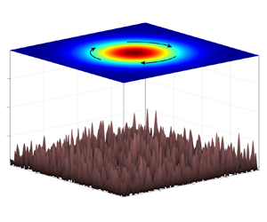
Particularly relevant to the present investigation are the findings of Gulliver & Radko (Reference Gulliver and Radko2022), who analysed the effects of irregular topography on the stability and longevity of ocean rings. This study explored the parameter regime in which the lateral extent of primary flows greatly exceeded that of individual topographic features – the configuration aptly dubbed the ‘sandpaper model’. The name was chosen to invoke the associations with fine abrasive particles of sandpaper that may be individually insignificant but have a tangible cumulative effect in grinding down much larger objects. A series of simulations in Gulliver & Radko (Reference Gulliver and Radko2022) revealed dramatic dissimilarities in the evolution of coherent vortices in flat-bottom basins and in the presence of realistic topographic patterns. The set-up of these experiments is illustrated by the schematic diagram in figure 1. We shall revisit this configuration in the present study (§ 4) to validate the theoretical descriptions of topographic effects.

Figure 1. Schematic diagram illustrating the set-up of the sandpaper model. The upper plane shows the streamfunction pattern of a large-scale vortex spinning above the irregular sea floor.
The present work attempts to further develop the sandpaper model by (i) identifying the dominant physical mechanisms controlling the flow/topography interaction and (ii) developing an explicit analytical description of the large-scale effects of bottom roughness. The principal theoretical challenge in this endeavour is to connect the statistical properties of bathymetry with the associated forcing of large-scale flows. One of the pragmatic outcomes could be an improved representation of unresolved topography-induced processes in coarse-resolution numerical models. This development, in turn, is expected to enhance the fidelity of global climate simulations at millennial time scales, which still fall short of fully resolving mesoscale components despite continuous advancements in high-performance computing.
To this end, the present investigation explores the influence of mesoscale topographic features on basin-scale  $({\sim} 1000\;\textrm{km})$ circulation patterns. Analytical progress is achieved by employing techniques of multiscale homogenization theory, a highly effective and widely used approach that is reviewed, for instance, by Mei & Vernescu (Reference Mei and Vernescu2010). Multiscale models represent the interaction of processes operating on dissimilar scales using multiple sets of spatial and temporal variables (e.g. Gama, Vergassola & Frisch Reference Gama, Vergassola and Frisch1994; Manfroi & Young Reference Manfroi and Young1999, Reference Manfroi and Young2002; Novikov & Papanicolau Reference Novikov and Papanicolau2001; Balmforth & Young Reference Balmforth and Young2002, Reference Balmforth and Young2005; Radko Reference Radko2011a,Reference Radkob). The key step in the development of such models is the derivation of solvability conditions that describe the evolution of the system entirely on large scales. Strictly speaking, this approach assumes substantial scale separation between interacting components, which may not always be realized in nature. However, multiscale models are known to be consistently accurate even in cases where scale separation is not pronounced or virtually non-existent (Radko Reference Radko2016, Reference Radko2020; Radko & Kamenkovich Reference Radko and Kamenkovich2017). Another attractive feature of multiscale methods is that they are based directly on governing equations. Therefore, such methods do not require empirical parameterizations and ad hoc assumptions, commonly used in other analytical approaches. As a result, the evolutionary large-scale models they produce are expected to be robust and dynamically transparent.
There have already been several promising attempts to address the flow/topography interaction problems using multiscale techniques (e.g. Bobrovich & Reznik Reference Bobrovich and Reznik1999; Reznik & Tsybaneva Reference Reznik and Tsybaneva1999; Radko & Kamenkovich Reference Radko and Kamenkovich2017; Radko Reference Radko2020). Much progress was made in modelling large-scale effects of one-dimensional bathymetry (e.g. Benilov Reference Benilov2000, Reference Benilov2001; Vanneste Reference Vanneste2003), which permits a fully analytical description of small-scale processes. The representation of more realistic irregular two-dimensional topographic features is more challenging and explicit solutions have been derived only for special cases (e.g. Vanneste Reference Vanneste2000; Goldsmith & Esler Reference Goldsmith and Esler2021). In the present study, we develop a new and sufficiently general multiscale model that leads to a closed set of large-scale equations. Tractability is achieved by identifying two dynamically distinct spatial scales and focusing the analysis on the corresponding oceanographically relevant asymptotic sector of the parameter space. This procedure is illustrated by applying it to the observationally derived spectrum of bathymetry (Goff & Jordan Reference Goff and Jordan1988). To validate the resulting parameterization, we consider the problem of the topographic spin-down of a large-scale circular vortex. The close agreement of the topography-resolving and corresponding parametric numerical solutions instils confidence in the efficacy of the proposed approach.
The manuscript is organized as follows. Section 2 describes the model configuration and governing equations. The multiscale theory is presented in § 3. The resulting parameterization of mesoscale topographic processes is implemented in a numerical model, which is used to simulate the spin-down of a large-scale vortex (§ 4). The parametric solutions are then compared with their topography-resolving counterparts. The results are summarized, and conclusions are drawn, in § 5.
2. Formulation
The minimal framework for the analysis of the interaction of large-scale barotropic flows with topography is the quasi-geostrophic rigid-lid model (e.g. Pedlosky Reference Pedlosky1987):
 \begin{equation}\frac{{\partial {\nabla ^2}{\psi ^\ast }}}{{\partial {t^\ast }}} + J({\psi ^\ast },{\nabla ^2}{\psi ^\ast }) + {\beta ^\ast }\frac{{\partial {\psi ^\ast }}}{{\partial {x^\ast }}} + \frac{{f_0^\ast }}{{H_0^\ast }}J({\psi ^\ast },{\eta ^\ast }) = {\nu ^\ast }{\nabla ^4}{\psi ^\ast } - {\gamma ^\ast }{\nabla ^2}{\psi ^\ast },\end{equation}
where  ${\psi ^\ast }$ is the streamfunction associated with the velocity field
  $({u^\ast },{v^\ast }) = ( - \partial {\psi ^\ast }/\partial {y^\ast },\partial {\psi ^\ast }/\partial {x^\ast })$,
  ${\eta ^\ast }$ is the depth variation, J is the Jacobian,
  ${\nu ^\ast }$ is the lateral eddy viscosity and
  ${\gamma ^\ast }$ is the Ekman bottom drag coefficient. The constant reference values of the ocean depth and the Coriolis parameter are denoted by
  $H_0^\ast $ and
  $f_0^\ast $, respectively, and
  ${\beta ^\ast } \equiv \partial {f^\ast }/\partial {y^\ast }$ is the meridional gradient of planetary vorticity. The asterisks hereafter represent dimensional quantities.
This study is focused on the interaction of large-scale flow patterns of the lateral extent  $O({L^\ast })$ with much smaller scales
  $O(L_S^\ast )$ that are present in topography. We assume that these small scales are limited to a finite range
  $L_{min}^\ast < L_S^\ast < L_C^\ast $. The range of small scales is constrained from below to ensure that the dynamics of all flow components is adequately represented by the quasi-geostrophic model. Thus, the Rossby numbers, including those based on the small scales
  $(R{o_S})$, must be much less than unity:
 \begin{equation}R{o_S} = \frac{{{U^\ast }}}{{f_0^\ast L_S^\ast }} \ll 1,\end{equation}
where  ${U^\ast }$ is the representative velocity. To conform to this requirement, our analysis targets the intermediate range of topographic scales that satisfy the inequality
 \begin{equation}\frac{{{U^\ast }}}{{f_0^\ast }} \ll L_{min}^\ast < L_S^\ast < L_C^\ast{\ll} {L^\ast }.\end{equation}
 The number of controlling parameters is reduced by non-dimensionalizing variables  ${\psi ^\ast }$,
  ${x^\ast }$,
  ${y^\ast }$ and
  ${t^\ast }$ using
  ${U^\ast }$ and
  ${L^\ast }$ as the units of velocity and length, respectively:
 \begin{equation}{\psi ^\ast } = {U^\ast }{L^\ast }\psi ,\quad {x^\ast } = {L^\ast }x,\quad {y^\ast } = {L^\ast }y,\quad {t^\ast } = \frac{{{L^\ast }}}{{{U^\ast }}}t.\end{equation}
For convenience, the depth variation is non-dimensionalized in a different manner:
 \begin{equation}{\eta ^\ast } = \frac{{{U^\ast }H_0^\ast }}{{f_0^\ast {L^\ast }}}\eta .\end{equation}
To be specific, we assume the following representative oceanic values of relevant scales:
 \begin{equation} {U^\ast } = 0.1\;\textrm{m}\ {\textrm{s}^{ - 1}},\quad {L^\ast } = {10^6}\;\textrm{m},\quad H_0^\ast= 4000\;\textrm{m},\quad f_0^\ast= {10^{ - 4}}\;\textrm{s}{}^{-1}.\end{equation}
The non-dimensionalization in (2.4) and (2.5) reduces the governing equation (2.1) to
 \begin{equation}\frac{{\partial {\nabla ^2}\psi }}{{\partial t}} + J(\psi ,{\nabla ^2}\psi ) + \beta \frac{{\partial \psi }}{{\partial x}} + J(\psi ,\eta ) = \nu {\nabla ^4}\psi - \gamma {\nabla ^2}\psi ,\end{equation}
where
 \begin{equation}\beta = \frac{{{L^\ast }^2}}{{{U^\ast }}}{\beta ^\ast },\quad \nu = \frac{{{\nu ^\ast }}}{{{U^\ast }{L^\ast }}},\quad \gamma = \frac{{{L^\ast }}}{{{U^\ast }}}{\gamma ^\ast }.\end{equation}
To explore the interaction between flow components of large and small lateral extent, we introduce the scale-separation parameter
 \begin{equation}\varepsilon = \frac{{L_C^\ast }}{{{L^\ast }}} \ll 1.\end{equation}
This parameter is used to define the new set of spatial and temporal scales  $({x_S},{y_S})$ that reflect the dynamics of small-scale processes. These variables are related to the original ones through
 \begin{equation}({x_S},{y_S}) = {\varepsilon ^{ - 1}}(x,y),\end{equation}
and the spatial derivatives in the governing system (2.7) are replaced accordingly:
 \begin{equation}\frac{\partial }{{\partial x}} \to \frac{\partial }{{\partial x}} + {\varepsilon ^{ - 1}}\frac{\partial }{{\partial {x_S}}},\quad \frac{\partial }{{\partial y}} \to \frac{\partial }{{\partial y}} + {\varepsilon ^{ - 1}}\frac{\partial }{{\partial {y_S}}}.\end{equation}
We assume that  $\beta $ and
  $\gamma $ are O(1) quantities, whilst the lateral viscosity
  $(\nu )$ is small and therefore rescaled in terms of
  $\varepsilon $:
 \begin{equation}\nu = {\varepsilon ^2}{\nu _0}.\end{equation}
Equation (2.12) implies that friction could be significant on small scales but its direct impact on the large-scale dynamics is weak.
Topographic patterns considered in the following model vary on both large and small scales:
 \begin{equation}\eta = {\eta _L}(x,y) + {\eta _S}({x_S},{y_S}).\end{equation}
In practical applications, the decomposition of bathymetry into the small- and large-scale components requires a specific prescription. The most natural approach – and the one that will be used in the present study (§ 4) – is based on the Fourier transform of  $\eta $:
 \begin{equation}\eta = \frac{1}{{\sqrt {\varDelta k\varDelta l} }}\iint {\tilde{\eta }(k,l)\,\textrm{exp}(\textrm{i}kx + \textrm{i}ly)\,\textrm{d}k\,\textrm{d}l} ,\end{equation}
where  $(k,l)$ are the wavenumbers in x and y, respectively, and tildes hereafter denote Fourier images. Note the normalization factor
  $1/\sqrt {\varDelta k\varDelta l} $ in the definition of Fourier transform, where
  $(\varDelta k,\varDelta l) = (2{\rm \pi} L_x^{ - 1},2{\rm \pi} L_y^{ - 1})$, and
  $({L_x},{L_y})$ is the domain size. This factor is introduced to ensure that the Parseval identity, to be used in subsequent developments, takes a convenient form:
 \begin{equation}{\langle ab\rangle _{x,y}} = \iint {\tilde{a} \textrm{conj}(\tilde{b})\,\textrm{d}k\,\textrm{d}l} .\end{equation}
Angle brackets hereafter represent mean values, with the averaging variables listed in the subscript.
Since the Fourier transform is linear, it can be conveniently separated into the contributions from high and low wavenumber as follows:
 \begin{align} \eta & = \underbrace{{\dfrac{1}{{\sqrt {\varDelta k\varDelta l} }}\iint\limits_{\kappa < 2{\rm \pi} /{L_C}} {\tilde{\eta }(k,l)\,\textrm{exp}(\textrm{i}kx + \textrm{i}ly)\,\textrm{d}k\,\textrm{d}l} }}_{{{\eta _L}}} \nonumber\\ & \quad + \underbrace{{\dfrac{1}{{\sqrt {\varDelta k\varDelta l} }}\iint\limits_{\kappa > 2{\rm \pi} /{L_C}} {\tilde{\eta }(k,l)\,\textrm{exp}(\textrm{i}kx + \textrm{i}ly)\,\textrm{d}k\,\textrm{d}l} }}_{{{\eta _S}}}, \end{align}
where  $\kappa \equiv \sqrt {{k^2} + {l^2}} $. The
  ${\eta _L}$ component of decomposition (2.16) gently varies on relatively large scales, and
  ${\eta _S}$ represents small-scale variability. The choice of the cutoff wavelength
  $({L_C} \ll 1)$ is necessarily problem-dependent.
For representative magnitudes of depth variation  ${\eta ^\ast }\sim 300\;\textrm{m}$ (Goff & Jordan Reference Goff and Jordan1988; Goff Reference Goff2020), their non-dimensional counterparts significantly exceed unity:
  $\eta \sim 75\,.$ This variability is mostly associated with relatively small spatial scales (100 km or less), which motivates rescaling the small-scale depth variation as
 \begin{equation}{\eta _S} = {\varepsilon ^{ - 1}}{\eta _0}.\end{equation}
We note in passing that the sought-after expression for the topographic forcing can also be obtained by considering the asymptotic sector with  ${\eta _S} = O(1)$, albeit in a more complicated manner. Here, we present the simplest derivation based on (2.17).
Using (2.11)–(2.13) and (2.17), the governing equation (2.7) is expressed in terms of the entire set of independent variables:
 \begin{equation}\left. {\begin{array}{*{20}{l@{}}} \begin{array}{l} \dfrac{{\partial \varsigma }}{{\partial t}} + J(\psi ,\varsigma ) + {\varepsilon^{ - 1}}{J_{{x_S},y}}(\psi ,\varsigma ) + {\varepsilon^{ - 1}}{J_{x,{y_S}}}(\psi ,\varsigma ) + {\varepsilon^{ - 2}}{J_{{x_S},{y_S}}}(\psi ,\varsigma ) + J(\psi ,{\eta_L})\\ \quad + {\varepsilon^{ - 3}}{J_{{x_S},{y_S}}}(\psi ,{\eta_0}) + \beta \dfrac{{\partial \psi }}{{\partial x}} + {\varepsilon^{ - 1}}\beta \dfrac{{\partial \psi }}{{\partial {x_S}}} = {\varepsilon^2}{\nu_0}{\nabla^2}\varsigma - \gamma \varsigma , \end{array}\\ {\varsigma = {\nabla^2}\psi ,\quad \nabla \equiv \frac{{{\partial^2}}}{{\partial {x^2}}} + 2{\varepsilon^{ - 1}}\frac{{{\partial^2}}}{{\partial x\partial {x_S}}} + {\varepsilon^{ - 2}}\frac{{{\partial^2}}}{{\partial x_S^2}} + \frac{{{\partial^2}}}{{\partial {y^2}}} + 2{\varepsilon^{ - 1}}\frac{{{\partial^2}}}{{\partial y\partial {y_S}}} + {\varepsilon^{ - 2}}\frac{{{\partial^2}}}{{\partial y_S^2}},} \end{array}} \right\}\end{equation}
where  $\varsigma $ is vorticity,
  ${J_{{x_S},{y_S}}}(a,b) \equiv (\partial a/\partial {x_S})(\partial b/\partial {y_S}) - (\partial a/\partial {y_S})(\partial b/\partial {x_S})$ denotes the Jacobian in
  $({x_S},{y_S})\,,$while
  ${J_{{x_S},y}}$ and
  ${J_{x,{y_S}}}$are based on
  $({x_S},y)$ and
  $(x,{y_S})\,,$respectively.
3. Multiscale model
We now proceed to develop a parametric version of the sandpaper model. To represent the interaction of large-scale circulation patterns with small-scale topography, the solution for  $\psi$ is sought in terms of power series in
  $\varepsilon \ll 1$:
 \begin{equation}\psi = {\psi _0}(x,y,t) + \varepsilon {\psi _1}(x,y,{x_S},{y_S},t) + {\varepsilon ^2}{\psi _2}(x,y,{x_S},{y_S},t) + \cdots. \end{equation}
The expansion opens with a large-scale pattern  ${\psi _0}$ that does not vary on small scales.
Series (3.1) are substituted in (2.18), and terms of the same order in  $\varepsilon $ are combined. The leading-order balance, which is realized at
  $O({\varepsilon ^{ - 2}})\,,$ is solved by assuming the steady small-scale pattern
  ${\psi _1}({x_S},{y_S})$ that satisfies
 \begin{equation}\nabla _S^2{\psi _1} + {\eta _0}({x_S},{y_S}) = 0,\end{equation}
where  $\nabla _S^2 \equiv {\partial ^2}/\partial x_S^2 + {\partial ^2}/\partial y_S^2$. The solution for
  ${\psi _1}$ can be readily obtained for any given pattern of topography by inverting the Laplacian in (3.2).
As discussed in Radko (Reference Radko2020), balance (3.2) represents the small-scale homogenization of the net potential vorticity (PV):
 \begin{equation}q = {\nabla ^2}\psi + \eta + \beta y.\end{equation}
The PV homogenization controls the dynamics of numerous geophysical systems (e.g. Rhines & Young Reference Rhines and Young1982; Dewar Reference Dewar1986; Marshall, Williams & Lee Reference Marshall, Williams and Lee1999) and is the cornerstone of the present model as well.
The  $O({\varepsilon ^{ - 1}})$ balance is
 \begin{equation}\left( {\frac{{\partial {\psi_0}}}{{\partial x}} + \frac{{\partial {\psi_1}}}{{\partial {x_S}}}} \right)\frac{{\partial {\varsigma _2}}}{{\partial {y_S}}} - \left( {\frac{{\partial {\psi_0}}}{{\partial y}} + \frac{{\partial {\psi_1}}}{{\partial {y_S}}}} \right)\frac{{\partial {\varsigma _2}}}{{\partial {x_S}}} = {\nu _0}\nabla _S^4{\psi _1} - \gamma \nabla _S^2{\psi _1},\end{equation}
where  ${\varsigma _2} \equiv \nabla _S^2{\psi _2}$, and the
  $O(1)$ balance amounts to
 \begin{align} & \dfrac{{\partial {\nabla ^2}{\psi _0}}}{{\partial t}} + J({\psi _0},{\nabla ^2}{\psi _0} + {\eta _L}) + \beta \dfrac{{\partial {\psi _0}}}{{\partial x}} + \gamma {\nabla ^2}{\psi _0} + \dfrac{{\partial {\psi _1}}}{{\partial {x_S}}}\dfrac{{\partial {\nabla ^2}{\psi _0}}}{{\partial y}}\nonumber\\ & \quad - \dfrac{{\partial {\psi _1}}}{{\partial {y_S}}}\dfrac{{\partial {\nabla ^2}{\psi _0}}}{{\partial x}} + \beta \dfrac{{\partial {\psi _1}}}{{\partial {x_S}}} - {\nu _0}\nabla _S^4{\psi _2} + \gamma \nabla _S^2{\psi _2} + \dfrac{{\partial \nabla _S^2{\psi _2}}}{{\partial t}} + \dfrac{{\partial {\psi _2}}}{{\partial {x_S}}}\dfrac{{\partial \nabla _S^2{\psi _2}}}{{\partial {y_S}}}\nonumber\\ & \quad - \dfrac{{\partial {\psi _2}}}{{\partial {y_S}}}\dfrac{{\partial \nabla _S^2{\psi _2}}}{{\partial {x_S}}} + \left( {\dfrac{{\partial {\psi_0}}}{{\partial x}} + \dfrac{{\partial {\psi_1}}}{{\partial {x_S}}}} \right)\dfrac{{\partial \nabla _S^2{\psi _3}}}{{\partial {y_S}}} - \left( {\dfrac{{\partial {\psi_0}}}{{\partial y}} + \dfrac{{\partial {\psi_1}}}{{\partial {y_S}}}} \right)\dfrac{{\partial \nabla _S^2{\psi _3}}}{{\partial {x_S}}}\nonumber\\ & \quad + \left( {\dfrac{{\partial {\psi_0}}}{{\partial x}} + \dfrac{{\partial {\psi_1}}}{{\partial {x_S}}}} \right)\left( {\dfrac{{{\partial^3}{\psi_2}}}{{\partial x_S^2\partial y}} + 2\dfrac{{{\partial^3}{\psi_2}}}{{\partial {x_S}\partial {y_S}\partial x}} + 3\dfrac{{{\partial^3}{\psi_2}}}{{\partial y_S^2\partial y}}} \right)\nonumber\\ & \quad - \left( {\dfrac{{\partial {\psi_0}}}{{\partial y}} + \dfrac{{\partial {\psi_1}}}{{\partial {y_S}}}} \right)\left( {3\dfrac{{{\partial^3}{\psi_2}}}{{\partial x_S^2\partial x}} + 2\dfrac{{{\partial^3}{\psi_2}}}{{\partial {x_S}\partial {y_S}\partial y}} + \dfrac{{{\partial^3}{\psi_2}}}{{\partial y_S^2\partial x}}} \right) = 0. \end{align}
The evolutionary large-scale equation is obtained as a solvability condition by averaging (3.5) in small-scale variables, which yields
 \begin{equation}\frac{{\partial {\nabla ^2}{\psi _0}}}{{\partial t}} + J({\psi _0},{\nabla ^2}{\psi _0} + {\eta _L}) + \beta \frac{{\partial {\psi _0}}}{{\partial x}} + D + \gamma {\nabla ^2}{\psi _0} = 0,\end{equation}
where
 \begin{equation}D = {\left\langle {\frac{{\partial {\psi_1}}}{{\partial {x_S}}}\frac{{\partial {\varsigma_2}}}{{\partial y}} - \frac{{\partial {\psi_1}}}{{\partial {y_S}}}\frac{{\partial {\varsigma_2}}}{{\partial x}}} \right\rangle _{{x_S},{y_S}}}.\end{equation}
Term D in (3.6) represents the topographic forcing of the large-scale flow by small-scale bottom roughness – the sought-after quantity in our analysis. The analytical developments detailed in Appendix A make it possible to eliminate  ${\varsigma _2}$ between (3.4) and (3.7), which leads to an explicit expression (A13) for D in terms of large-scale velocities.
At this point, the multiscale analysis is complete, and the rest of the material is presented in terms of original variables. To lighten up the notation, we omit the subscripts ‘0’ in describing the leading-order components, which reduces (A13) to
 \begin{equation}D = G\left( {\frac{\partial }{{\partial x}}\left( {\frac{v}{{{u^2} + {v^2}}}} \right) - \frac{\partial }{{\partial y}}\left( {\frac{u}{{{u^2} + {v^2}}}} \right)} \right),\end{equation}
where  $(u,v) = ( - \partial \psi /\partial y,\partial \psi /\partial x)$ and
 \begin{equation}G = 2{\rm \pi} \int {{{|{{{\tilde{\eta }}_S}} |}^2}\left( {\frac{\gamma }{\kappa } + \nu \kappa } \right)\textrm{d}\kappa } ,\quad \kappa = \sqrt {{k^2} + {l^2}} .\end{equation}
In (3.9),  $(k,l)$ are the wavenumbers, and
  ${\tilde{\eta }_S}$ represents the Fourier image of the small-scale component of topography.
Note that topographic forcing D in the evolutionary equation (3.6) originates from the averaged nonlinear advective term in the governing equation (2.1) and, therefore, represents the eddy-induced mixing of momentum. Thus, the essential role of topography in the sandpaper model is the generation of small-scale eddies, which affect large-scale flows through the associated Reynolds stresses. The topographic ‘form drag’ acting directly on primary flows, on the other hand, does not affect the large-scale circulation at the leading order.
Equation (3.8) suggests that the magnitude of topographic forcing generally decreases with the increasing speed of the large-scale flow. This peculiar inverse relation seems counterintuitive at first, as one expects the topography-induced drag to be more intense in swift currents. However, it can be physically rationalized by considering the advection--dissipation balance (3.4). The dissipative terms on its right-hand side are controlled by topography and are independent of the large-scale speed. Thus, to maintain the net advection, which is represented by the left-hand side of (3.4), an increase in flow speed should be compensated by the equivalent reduction in the magnitude of the perturbation  $({\varsigma _2})$. Weaker perturbations, in turn, imply weaker Reynolds stresses and smaller topographically induced drag.
It should also be emphasized that the coefficient G in the topographic forcing term (3.9) is uniquely determined by the bathymetric spectrum and the explicit dissipation parameters  $(\gamma ,\nu )$. Thus, (3.8)–(3.9) can be viewed as a rigorous parameterization of the effects of small-scale topography on large-scale circulation patterns. Another interesting feature revealed by the multiscale model is the catalytic nature of topographic forcing. Equation (3.9) indicates that G vanishes in the non-dissipative limit
  $(\nu ,\gamma ) = (0,0)$, and so does the forcing term (3.6). Thus, while bathymetry can dramatically amplify dissipative effects, the explicit frictional processes are essential for engaging the topographic spin-down mechanisms.
4. Spin-down of a large-scale vortex
To assess the skill of the sandpaper model (3.6) in representing the effects of small-scale bathymetric variability, we now perform a series of topography-resolving simulations and compare them with their parametric counterparts.
The spectrum of bottom topography for lateral scales of several hundred metres and more is adequately captured by the empirical representation of Goff & Jordan (Reference Goff and Jordan1988). Dimensionally, this spectrum is given by
 \begin{equation}P_\eta ^\ast= \frac{{{h^{{\ast} 2}}(\mu - 2)}}{{{{(2{\rm \pi} )}^3}k_0^\ast l_0^\ast }}\bigg(1 + \left(\frac{k^\ast}{2{\rm \pi} k_0^\ast }\right)^2 + \left(\frac{l^\ast }{2{\rm \pi} l_0^\ast}\right)^2\bigg)^{-\mu/2}.\end{equation}
According to Nikurashin et al. (Reference Nikurashin, Ferrari, Grisouard and Polzin2014), typical topographic patterns can be represented by the following parameters:
 \begin{equation}\mu = 3.5,\quad k_0^\ast= 1.8 \times {10^{ - 4}}\;{\textrm{m}^{ - 1}},\quad l_0^\ast= 1.8 \times {10^{ - 4}}\;{\textrm{m}^{ - 1}},\quad {h^\ast } = 305\;\textrm{m}\textrm{.}\end{equation}
For  $k_0^\ast= l_0^\ast $, the Goff–Jordan spectrum is isotropic and therefore satisfies all assumptions of the parametric model (§ 3).
After non-dimensionalization, (4.1) reduces to
 \begin{equation}{P_\eta } = C{\bigg( {1 + {{\left( {\frac{\kappa }{{2{\rm \pi} {L^\ast }k_0^\ast }}} \right)}^2}} \bigg)^{ - \mu /2}},\quad C = \frac{{\mu - 2}}{{{{(2{\rm \pi} )}^3}}}{\left( {\frac{{f_0^\ast {h^\ast }}}{{{U^\ast }H_0^\ast k_0^\ast }}} \right)^2}.\end{equation}
To construct topographic patterns that conform to the Goff–Jordan spectrum, we prescribe the Fourier image of topography  $(\tilde{\eta })$ as follows:
 \begin{equation}\tilde{\eta } = \sqrt {{P_\eta }} \exp (\textrm{i}\varphi ),\end{equation}
where randomly generated distributions are used for the phase  $\varphi = \varphi (k,l)$. The only constraint that we impose on
  $\varphi $ is that of antisymmetry:
  $\varphi (k,l) ={-} \varphi ( - k, - l)$, which ensures that
  $\eta $ is real. The patterns of
  $\eta (x,y)$ designed in this manner are used in all subsequent examples.
To quantify and further explore the effects of small-scale bathymetry on large-scale flows, we turn to the vortex spin-down model illustrated in figure 1. The large-scale circulation is initiated using the Gaussian streamfunction pattern – a common choice in theoretical and numerical models of coherent vortices (e.g. Early, Samelson & Chelton Reference Early, Samelson and Chelton2011; Sutyrin & Radko Reference Sutyrin and Radko2019):
 \begin{equation}{\psi _G} = \exp ( - {r^2}),\quad r = \sqrt {{x^2} + {y^2}} .\end{equation}
Without loss of generality, the effective non-dimensional radius is set to unity. To accurately represent the vortex evolution, it is important to ensure that the relevant dynamics is captured by the quasi-geostrophic model (2.7). The quasi-geostrophic approximation is appropriate for flows with low Rossby numbers (2.2), which excludes structures that are exceedingly swift and narrow. Therefore, we impose an upper limit on the range of wavenumbers contained in the bathymetric spectrum:
 \begin{equation}\kappa < {\kappa _{max}} = \frac{{2{\rm \pi} }}{{{L_{min}}}}.\end{equation}
The minimal spatial scale of bathymetry is set to  ${L_{min}} = 0.01$, which is dimensionally equivalent to
  $L_{min}^\ast= 10\;\textrm{km}$. This restriction ensures that the maximal Rossby numbers, estimated here as
 \begin{equation}R{o_{max}} = \mathop {\max }\limits_{x,y,t} \left( {\frac{{|{{\nabla^2}{\psi^\ast }} |}}{{f_0^\ast }}} \right)\end{equation}
do not exceed  $R{o_{max}} = 0.2$ in any of the presented experiments.
The following simulations are performed using the de-aliased pseudo-spectral model employed in our previous works (e.g. Sutyrin & Radko Reference Sutyrin and Radko2019; Radko Reference Radko2021). To limit the effects of doubly periodic boundary conditions on vortex evolution, we use a relatively wide computational domain of size  $({L_x},{L_y}) = (8,8)\,.$ The topography-resolving simulations employ a fine mesh with
  $({N_x},{N_y}) = (6144,6144)$ grid points. In our baseline configuration, the bottom drag coefficient is assigned a value of
  $\gamma = 0.01$ and the lateral viscosity is
  $\nu = {10^{ - 4}}$. Motivated by the considerations of simplicity, we ignore the beta effect
  $(\beta = 0)$.
Our first experiment  $(ExpR)$ explores the configuration in which scales of topography and the dominant flow pattern are clearly separated, thereby conforming to the design of the multiscale model (§ 3). To this end, we introduce the cutoff scale of
  ${L_C} = 0.1$ and exclude from the topographic spectrum (4.3) all spectral components with wavelengths exceeding
  ${L_C}$:
 \begin{equation}\kappa > {\kappa _{min}} = \frac{{2{\rm \pi} }}{{{L_C}}}.\end{equation}
Such filtering is equivalent to setting the small parameter of the multiscale model to  ${\varepsilon = 0.1}$.
Figure 2(a,b) shows the streamfunction patterns in  $ExpR$ at
  $t = 0$ and
  $t = 1$, respectively, revealing a rapid and substantial (~50%) reduction in the vortex intensity. To better illustrate the pattern of small-scale flow features, figure 2(c) shows the vorticity
  $\varsigma = {\nabla ^2}\psi $ at
  $t = 1$ in a small region
  $(\varOmega )$ in the vortex interior, where
 \begin{equation}\varOmega = \{ 0.5 < x < 0.6,\;0.5 < y < 0.6\} .\end{equation}
The most striking feature of the vorticity distribution (figure 2c) is its strong anticorrelation with the corresponding pattern of topography (figure 2d), with a correlation coefficient of  ${r_{corr}} ={-} 0.97$. Vorticity and topography essentially mirror each other
  $(\varsigma \approx{-} \eta )\,,$ which reflects the homogenization tendency of the net PV (3.3). This tendency represents the cornerstone of the multiscale theory (§ 3) and is captured by the leading-order asymptotic balance (3.2).

Figure 2. The topography-resolving experiment  $ExpR$ in which the bathymetric spectrum is restricted to relatively small-scale components
  $(2{\rm \pi} {\kappa ^{ - 1}} < {L_C} = 0.1)$. Panels (a) and (b) show the streamfunction patterns at
  $t = 0$ and
  $t = 1$, respectively. Panels (c) and (d) present enlarged views of the vorticity
  $(\varsigma )$ and depth perturbation
  $(\eta )$ in the small area (4.9).
In the next example (figure 3), the spectrum of bathymetry is not restricted to small scales. This unrestricted experiment  $(ExpU)$ represents a much more stringent test of the parametric model. The entire development of the asymptotic theory (§ 3) is based on the expansion in the small parameter
  $(\varepsilon )$ quantifying the scale separation. Thus, the analysis of
  $ExpU$ will make it possible to determine whether the scale-separation requirement
  $(\varepsilon \ll 1)$ is essential for the fidelity of our theory-based parameterizations. The instantaneous patterns of the streamfunction at
  $t = 1$ and 2 in this simulation are shown in figures 3(a) and 3(b) respectively. Adding large-scale bathymetric components visibly affects the flow patterns (cf. figures 2b and 3a) making them more irregular and asymmetric. Nevertheless, the average intensities of flows realized in the experiments in figures 2 and 3 at corresponding stages are comparable.

Figure 3. The streamfunction patterns realized in the topography-resolving experiment  $ExpU$ at
  $t = 1$ and
  $t = 2$ are shown in (a) and (b), respectively.
We now go on to determine whether the flow evolution in the foregoing topography-resolving experiments is captured by the parametric model. However, two technical issues must be addressed before performing parametric simulations. First, the topographic forcing term (3.8) is singular in locations where the absolute velocity  $V = \sqrt {{u^2} + {v^2}} $ is zero, which hinders numerical integrations of the parametric model. This problem is mitigated by introducing the modified velocity
 \begin{equation}{V_m} = \frac{V}{{{{\tanh }^2}(\delta V)}},\end{equation}
where  $\delta \gg 1$. While
  ${V_m} \approx V$ for most of the vortex area, (4.10) guarantees that the modified velocity is non-zero at any given point. The expression for D is adjusted accordingly:
 \begin{equation}{D_m} = G\left( {\frac{\partial }{{\partial x}}\left( {\frac{v}{{V{V_m}}}} \right) - \frac{\partial }{{\partial y}}\left( {\frac{u}{{V{V_m}}}} \right)} \right),\end{equation}
which regularizes its singular pattern and ensures that the topographic forcing term vanishes in quiescent regions  $(V \to 0)$. Extensive experimentation with the parametric model revealed that the results are not sensitive to the choice of
  $\delta $ as long as it greatly exceeds unity. However, excessively large values of
  $\delta $ are associated with the appearance of sharp features in the flow field that demand high resolution. In all parametric simulations presented here, we used
  $\delta = 25$, which made these experiments both accurate and efficient.
Another complication is that the leading-order vorticity equation (3.6) does not include small lateral dissipation  $(\nu {\nabla ^2}\psi )$ since it appears at
  $O({\varepsilon ^2})$ in the expansion. However, lateral viscosity is needed to control the numerical stability of simulations, and therefore it is now reintroduced in the parametric model:
 \begin{equation}\frac{{\partial {\nabla ^2}\psi }}{{\partial t}} + J(\psi ,{\nabla ^2}\psi + {\eta _L}) + \beta \frac{{\partial \psi }}{{\partial x}} + {D_m} + \gamma {\nabla ^2}\psi = \nu {\nabla ^4}\psi .\end{equation}
 The parametric integrations were performed using a pseudo-spectral model that, aside from the inclusion of the topographic forcing term  ${D_m}$ in the vorticity equation (4.12), is identical to the one used for topography-resolving experiments. The coefficient G in (3.9) is readily evaluated for the Goff–Jordan spectrum:
 \begin{equation}G = 2{\rm \pi} \int\limits_{{\kappa _{min}}}^{{\kappa _{max}}} {C{{\bigg( {1 + {{\left( {\frac{\kappa }{{2{\rm \pi} {L^\ast }k^*_0}}} \right)}^2}} \bigg)}^{ - \mu /2}}\left( {\frac{\gamma}{\kappa} + \nu \kappa } \right)\textrm{d}\kappa .}\end{equation}
For the controlling parameters  $(\nu ,\gamma ,{\kappa _{min}},{\kappa _{max}})$ used in
  $ExpR$, (4.13) yields
 \begin{equation}G = 0.1050,\end{equation}
and the corresponding parametric simulation is referred to as  $ExpRP$. For the experiment
  $ExpU$, in which the range of wavenumbers in
  $\eta $ is not restricted from below, we assign
  ${\kappa _{min}}$ the value based on the size of the computational domain
  ${\kappa _{min}} = 2{\rm \pi} /{L_y}$. This only slightly increases G to
 \begin{equation}G = 0.1067,\end{equation}
and the corresponding parametric simulation is referred to as  $ExpUP$. Finally, we have also performed a hybrid experiment
  $(ExpHP)$ in which large-scale components
  $(2{\rm \pi} {\kappa ^{ - 1}} > {L_C} = 0.1)$ of the Goff–Jordan spectrum are resolved and the small scales
  $(2{\rm \pi} {\kappa ^{ - 1}} < {L_C})$ are parameterized. Since parametric simulations do not require the resolution of small-scale bathymetry, they can be performed on relatively coarse meshes. The simulations employing grids as small as
  $({N_x},{N_y}) = (384,384)$ are very close to their better-resolved counterparts. In the following examples, we use
  $({N_x},{N_y}) = (3072,3072)$.
To systematically compare the topography-resolving and parametric simulations, we present (figure 4) the corresponding temporal records of the mean kinetic energy  ${E_k} = 0.5{\langle {|{\nabla \psi } |^2}\rangle _{x,y}}$. All experiments are remarkably consistent in predicting a rapid, nearly exponential topography-induced decay of energy. By
  $t = 4\,,$
  ${E_k}$ is reduced by more than four orders of magnitude relative to its initial level. In contrast, the energy dissipation in the corresponding flat-bottom simulation
  $(Exp0)$, also shown in figure 4, is much slower. Over the same period, kinetic energy there reduces merely by 8%. This dissimilarity illustrates the dramatic impact of the bottom roughness on the evolution of large-scale circulation patterns.

Figure 4. The time series of mean kinetic energy ( ${E_k}$) in the topography-resolving (
 $ExpR$ and
  $ExpU$) and parametric (
 $ExpRP$,
  $ExpUP$ and
  $ExpHP$) experiments. Also shown is the record of
  ${E_k}(t)$ in the corresponding flat-bottom simulation
  $(Exp0)$.
Figure 5 presents the azimuthally averaged velocity patterns  ${V_{av}}(r)$ realized at various times. The experiments in which topographic spectra are restricted to relatively small scales (
 $ExpR$ and
  $ExpRP$) are shown in figure 5(a). Figure 5(b) combines all unrestricted-topography simulations (
 $ExpU$,
  $ExpUP$ and
  $ExpHP$). These diagnostics, once again, demonstrate the general consistency of the topography-resolving and parametric simulations, lending credence to the multiscale theory developed in § 3.

Figure 5. The radial profiles of the azimuthally averaged absolute velocity  ${V_{av}}(r)$ at
  $t = 1$, 2 and 3 are indicated by blue, red and black curves, respectively. (a) Presents experiments in which the bathymetric spectrum is restricted to relatively small-scale components (
 $ExpR$ and
  $ExpRP$). The profiles realized in unrestricted experiments
  $ExpU$,
  $ExpUP$ and
  $ExpHP$ are shown in (b).
Since the intensity of topographic forcing is ultimately determined by the explicit dissipation parameters, it also behoves us to explore the parameter space  $(\nu ,\gamma )$ with an eye on the vortex spin-down rates. To be specific, we shall focus on the decay of the kinetic energy. The foregoing simulations indicate that the patterns of
  ${E_k}(t)$ are nearly exponential (figure 4), and therefore the energy decay rate can be approximated by its initial value:
 \begin{equation}\lambda ={-} \frac{1}{{{E_k}}}{\left. {\frac{{\partial {E_k}}}{{\partial t}}} \right|_{t = 0}}.\end{equation}
The initial decay rate can be readily evaluated for any given values of  $(\nu ,\gamma )$ as follows. First, we form the energy equation by multiplying the parametric vorticity equation (4.12) by
  $\psi $ and averaging it in
  $(x,y)$. The result is simplified by integrating selected terms by parts, subject to periodic conditions at the boundaries of the computational domain, which yields
 \begin{equation}\frac{{\partial {E_k}}}{{\partial t}} = {\langle \psi {D_m} - \nu \psi {\nabla ^4}\psi + \gamma \psi {\nabla ^2}\psi \rangle _{x,y}}.\end{equation}
The topographic effects in (4.17) are represented by the first component on its right-hand side:
 \begin{equation}{E_{\eta t}} = {\langle \psi {D_m}\rangle _{x,y}}.\end{equation}
Using (4.11), we express this tendency as
 \begin{equation}{E_{\eta t}} ={-} G{\langle \sqrt {V\,V_m^{ - 1}} \rangle _{x,y}} < 0,\end{equation}
which proves that topography in our model has an invariably adverse effect on the intensity of large-scale flows. This is an important conclusion that should not be taken for granted since in some models (e.g. Holloway Reference Holloway1987) topography acts to reinforce, rather than resist, large-scale flows.
To further quantify the contribution of topography to vortex spin-down, the components of (4.17) are evaluated using the initial Gaussian state (4.5), arriving at
 \begin{equation}\lambda = 2\frac{{{{\langle \nu {\psi _G}{\nabla ^4}{\psi _G} - \gamma {\psi _G}{\nabla ^2}{\psi _G} - {\psi _G}{D_m}\rangle }_{x,y}}}}{{{{\langle {{|{\nabla {\psi_G}} |}^2}\rangle }_{x,y}}}}.\end{equation}
The resulting pattern of  $\lambda (\nu ,\gamma )$ is shown in figure 6(a). This plot reveals the relatively rapid linear increase in the decay rate with increasing lateral viscosity. The effects of bottom friction, on the other hand, are surprisingly limited. The two order of magnitude increase in
  $\gamma $ elevates
  $\lambda $ by less than 20%.

Figure 6. (a) The energy decay rate  $(\lambda )$ plotted as a function of dissipation parameters
  $\nu $ and
  $\gamma $. (b) The ratio of the topography-induced and flat-bottom energy decay rates
  $R(\nu ,\gamma )$.
It is also instructive to quantify the differences between the topography-induced decay rates and their flat-bottom counterparts. To this end, we compute the component of the decay rate that can be attributed solely to explicit dissipation:
 \begin{equation}{\lambda _0} = 2\frac{{{{\langle \nu {\psi _G}{\nabla ^4}{\psi _G} - \gamma {\psi _G}{\nabla ^2}{\psi _G}\rangle }_{x,y}}}}{{{{\langle {{|{\nabla {\psi_G}} |}^2}\rangle }_{x,y}}}}.\end{equation}
The ratio of the topography-induced and flat-bottom decay rates  $R = \lambda /{\lambda _0}$ is plotted in figure 6(b) as a function of
  $(\nu ,\gamma )$. It reveals a wide range of R values, which could be as high as
  ${10^3}$ or more. Such strong topographic intensification of the energy decay is remarkable, especially given the catalytic role played by bathymetry in the spin-down dynamics.
Finally, we assess the performance characteristics of the parametric model for various levels of small-scale depth variability. Oceanographic observations (Goff Reference Goff2020) reveal substantial geographic variability in the root-mean-square (r.m.s.) roughness height  ${\eta _{rms}} = \sqrt {{{\langle {\eta ^2}\rangle }_{x,y}}} $. In most of the ocean, it is limited to the range of
  $40\;\textrm{m} < \eta _{rms}^\ast < 400\;\textrm{m}$, which is equivalent to
 \begin{equation}10 < {\eta _{rms}} < 100\end{equation}
in non-dimensional units based on scales (2.6). To explore this range, we perform a series of simulations, both topography resolving and parametric, in which  ${\eta _{rms}}$ is systematically varied. These simulations are analogous to
  $ExpR$ and
  $ExpRP$ in all respects, except that in each run the topographic spectrum (4.3) is renormalized to produce the desired r.m.s. height. The vortex spin-down rates
  $(\lambda )$ are then evaluated from the best fit of the kinetic energy records
  ${E_k}(t)$ by the exponential patterns
  ${E_{fit}} = {E_0}\,\textrm{exp}( - \lambda t)$ and plotted as a function of
  ${\eta _{rms}}$ in figure 7. These results indicate that the parametric and topography-resolving simulations are remarkably consistent over the entire oceanographically relevant range (4.22). In all runs, the relative error of the multiscale model is less than 8%. It should also be emphasized that all values of
  $\lambda $ in figure 7 greatly exceed their flat-bottom counterpart
  $({\lambda _0} = 0.0201)$. Even for the smallest and rarely observed value of topographic height
  $({\eta _{rms}} = 10)$, bathymetry increases the decay rate by a factor of
  $R = 4.38$. For a more representative height of
  ${\eta _{rms}} = 100$, the amplification factor increases to
  $R = 352.5$.

Figure 7. The energy decay rate  $(\lambda )$ plotted as a function of the r.m.s. depth variation
  $({\eta _{rms}})$. Parametric simulations are shown in red, and the topography-resolving experiments are indicated by the black curve.
5. Discussion
This work explores the interaction of broad oceanic flows with irregular smaller-scale bathymetry – the configuration referred to as the sandpaper model. The analytical developments are based on the multiscale homogenization theory and lead to a closed set of large-scale equations. The resulting system represents a rigorous asymptotics-based parameterization of the flow forcing by the sea-floor roughness. Bathymetry is introduced in the multiscale theory by assuming a statistically representative spectral distribution of the ocean depth. The specific calculations are performed using the observationally derived spectrum of Goff & Jordan (Reference Goff and Jordan1988), and the associated theoretical predictions are validated by topography-resolving simulations.
All evidence, analytical and numerical, gathered in this investigation consistently points to a profound influence of topography on the dynamics of large-scale flows. For instance, we demonstrate that the topographic spin-down rates of a barotropic vortex can exceed those induced by explicit dissipation by as much as 2–3 orders of magnitude. This observation becomes particularly striking when we recall that the role of topography in the multiscale model is fundamentally catalytic: the leading-order topographic forcing term (D) vanishes in the non-dissipative limit.
Given such a strong adverse impact of irregular bathymetry on large-scale flows, one may wonder why it is seldom considered in theoretical and idealized numerical studies of ocean circulation. Traditionally, conceptual models have focused on the effects of the Ekman bottom drag and lateral friction (Stommel Reference Stommel1948; Munk Reference Munk1950). A natural development of the circulation theory should involve supplanting these direct dissipative processes with more efficient topographic spin-down mechanisms. Perhaps the lingering lack of progress in this direction can be attributed to the perceived complexity of governing equations in the presence of realistic bathymetry, which may impede analytical developments. In this regard, the concise representation of topographic effects by the sandpaper model may prove to be highly beneficial, opening new pathways for the advancement of the general circulation theory.
The present investigation has also brought some new insights into the physics of the topographic spin-down. The key strength of multiscale methods, such as employed in this study, is their dynamic transparency. The users can identify and interpret the entire sequence of cross-scale interactions by examining balances that arise at each order in the asymptotic expansion. Following this strategy, we conclude from the leading-order balance that the topographic spin-down is initiated by the homogenization of PV (e.g. Rhines & Young Reference Rhines and Young1982). The homogenization creates a stationary small-scale flow that is rigidly constrained by the topography. This pattern interacts with the large-scale current to produce a secondary perturbation that also contains fine structures but is modulated over large scales. Since these primary and secondary small-scale components are not orthogonal, their nonlinear interaction results in large-scale forcing. This finding implies that the spin-down of a large-scale flow in our model is caused solely by the lateral eddy mixing of momentum. The large-scale effects of topography are indirect and limited to the generation of a small-scale eddy field associated with considerable Reynolds stresses. In contrast, the topographic form drag acting directly on the large-scale current does not contribute to the spin-down at the leading order. Somewhat counterintuitively, the topography-induced stresses are inversely proportional to the large-scale speed, which can be rationalized by considering the advective--dissipative balance for the secondary perturbation.
It is also interesting that the small-scale homogenization of PV, which is borne out very clearly in both topography-resolving simulations and the asymptotic model, is seldom considered in multiscale flow--topography interaction theories (e.g. Vanneste Reference Vanneste2000, Reference Vanneste2003; Goldsmith & Esler Reference Goldsmith and Esler2021). The distinguishing feature of our approach is the focus on relatively swift large-scale currents. As they impinge on rapidly varying topography, homogenization allows Lagrangian particles to maintain their net PV without dramatic reorganization of the flow pattern. Slow flows, on the other hand, respond to the depth variation in a fundamentally different manner, by developing stationary Taylor columns that trap fluid in their interior (Taylor Reference Taylor1923; Johnson Reference Johnson1978). Thus, while our multiscale model accurately represents the dynamics of realistically fast oceanic flows, it may not be applicable in stagnant regions. The tell-tale sign of this limitation is the singularity of the expression for topographic forcing, which increases without bound with decreasing flow speed. In this regard, it would be highly desirable to develop a universal asymptotic model that can capture both slow and fast flow limits in a single framework.
Another notable outcome of this study is the assessment of the applicability and performance characteristics of the multiscale model itself. For instance, the model formally assumes a substantial separation between scales of the interacting flow components. However, we find that this condition may not be critical. Even the parametric simulation in which the entire spectrum of topography is treated as small-scale variability still offers a surprisingly accurate description of the flow field. The ability of the multiscale model to retain its predictive skill under such unfavourable conditions is encouraging. It indicates that the techniques developed here can be successfully applied to flows realized in nature, which usually lack clear-cut scale separation.
The present study can be extended in several ways. An obvious step towards realism would be the generalization of our analysis to baroclinic flows, more representative of typical oceanic circulation patterns. In this regard, the present homogeneous theory offers a convenient roadmap for the development of analogous multilayer and continuously stratified models. An even more significant undertaking would be the transition from the quasi-geostrophic framework to more general hydrodynamic models, such as the shallow-water and Navier–Stokes systems. The principal limitation of the quasi-geostrophic approximation is that it may inadequately represent submesoscale ( ${\sim} 10\;\textrm{km}$ or less) flow components. At the same time, such features remain largely unresolved by the current generation of general circulation models, which motivates the development of reliable parameterizations of submesoscale processes. Another benefit of adopting a more general framework is an opportunity to capture the effects of internal lee waves, which are a priori excluded in the quasi-geostrophic model. The topographic wave-induced drag is known to substantially affect the large-scale circulation of the ocean and remains a subject of keen interest in oceanography (Eden, Olbers & Eriksen Reference Eden, Olbers and Eriksen2021; Klymak et al. Reference Klymak, Balwada, Garabato and Abernathey2021). We believe that many pressing challenges in the flow--topography interaction theory can be met through the systematic application of multiscale methods, as illustrated here using the minimal spin-down model.
Acknowledgements
The author thanks N. Balmforth and the anonymous reviewers for helpful comments.
Funding
Support of the National Science Foundation (grant OCE 1828843) is gratefully acknowledged.
Declaration of interests
The author reports no conflict of interest.
Appendix A. Auxiliary steps in the development of the multiscale model
The following analysis leads to an explicit expression of the topographic forcing function (3.7) in terms of the properties of the large-scale flow. This is achieved by combining the advection--dissipation balance (3.4) and expression (3.7) in a manner that eliminates  ${\varsigma _2}$. We start with the transition to the flow-following small-scale coordinate system:
 \begin{equation}\left. {\begin{array}{*{20}{c@{}}} {{{x^{\prime}}_S} = {x_S}\,\textrm{cos}\,\theta + {y_S}\,\textrm{sin}\,\theta ,}\\ {{{y^{\prime}}_S} ={-} {x_S}\,\textrm{sin}\,\theta + {y_S}\,\textrm{cos}\,\theta .} \end{array}} \right\}\end{equation}
The flow-orientation variable  $\theta $ in (A1) is defined by
 \begin{equation}\cos (\theta ) = \frac{{{u_0}}}{{{V_0}}},\quad \sin (\theta ) = \frac{{{v_0}}}{{{V_0}}},\end{equation}
where  $({u_0},{v_0}) \equiv ( - \partial {\psi _0}/\partial y,\partial {\psi _0}/\partial x)$ and
  ${V_0} = \sqrt {u_0^2 + v_0^2}$. Note that components of (3.4) and (3.7) are invariant with respect to the transition to the flow-following frame of reference. Therefore, in the new coordinate system, (3.4) takes the form
 \begin{equation}{V_0}\frac{{\partial {\varsigma _2}}}{{\partial {{x^{\prime}}_S}}} + {J_{{{x^{\prime}}_S},{{y^{\prime}}_S}}}({\psi _1},{\varsigma _2}) = {\nu _0}\nabla ^{\prime4}_S{\psi _1} - \gamma \nabla ^{\prime2}_S{\psi _1},\end{equation}
and (3.7) is written as
 \begin{equation}D = \frac{\partial }{{\partial y}}({D_V}\,\textrm{cos}\,\theta - {D_U}\,\textrm{sin}\,\theta ) - \frac{\partial }{{\partial x}}({D_V}\,\textrm{sin}\,\theta + {D_U}\,\textrm{cos}\,\theta ),\end{equation}
where
 \begin{align}{D_V} = {\left\langle {\frac{{\partial {\psi_1}}}{{\partial {{x^{\prime}}_S}}}{\varsigma_2}} \right\rangle _{{{x^{\prime}}_S},{{y^{\prime}}_S}}},\quad {D_U} = {\left\langle {\frac{{\partial {\psi_1}}}{{\partial {{y^{\prime}}_S}}}{\varsigma_2}} \right\rangle _{{{x^{\prime}}_S},{{y^{\prime}}_S}}}\end{align}
Term  ${D_U}$ represents the effects associated with the eddy-induced mixing of vorticity in the direction of large-scale flow and it can be shown to be inconsequential based on its symmetries. For instance, reversing the x’-orientation of small-scale bathymetry
  ${\eta _S} \to {\eta _S}( - {x^{\prime}_S},{y^{\prime}_S})$ corresponds to reversing the vorticity sign
  ${\varsigma _2} \to - {\varsigma _2}( - {x^{\prime}_S},{y^{\prime}_S})$ and therefore reverses the sign of
  ${D_U}$. Thus, any statistical averaging that assigns equal weights to a given pattern of
  ${\eta _S}$ and its mirror image will result in the cancellation of the net contribution of individual realizations to
  ${D_U}$.
To obtain an explicit expression for  ${D_V}$, we integrate (A5) by parts:
  ${D_V} ={-} {\langle {\psi _1}(\partial {\varsigma _2}/\partial {x^{\prime}_S})\rangle _{{{x^{\prime}}_S},{{y^{\prime}}_S}}}$ and eliminate
  $\partial {\varsigma _2}/\partial {x^{\prime}_S}$ using (A3), which yields
 \begin{equation}{D_V} = \underbrace{{V_0^{ - 1}{{\langle {\psi _1}{J_{{{x^{\prime}}_S},{{y^{\prime}}_S}}}({\psi _1},{\varsigma _2})\rangle }_{{{x^{\prime}}_S},{{y^{\prime}}_S}}}}}_{{{D_J}}}\underbrace{{ - V_0^{ - 1}{\nu _0}{{\langle {\psi _1}\nabla ^{\prime4}_S{\psi _1}\rangle }_{{{x^{\prime}}_S},{{y^{\prime}}_S}}}}}_{{{D_\nu }}} + \underbrace{{V_0^{ - 1}\gamma {{\langle {\psi _1}\nabla ^{\prime2}_S{\psi _1}\rangle }_{{{x^{\prime}}_S},{{y^{\prime}}_S}}}}}_{{{D_\gamma }}}.\end{equation}
The first  $({D_J})$ component of (A6) is eliminated by virtue of the following identity:
 \begin{equation}{\langle {\psi _1}{J_{{{x^{\prime}}_S},{{y^{\prime}}_S}}}({\psi _1},{\varsigma _2})\rangle _{{{x^{\prime}}_S},{{y^{\prime}}_S}}} = {\left\langle {\frac{\partial }{{\partial {{x^{\prime}}_S}}}\left( {\frac{{\psi_1^2}}{2}\frac{{\partial {\varsigma_2}}}{{\partial {{y^{\prime}}_S}}}} \right) - \frac{\partial }{{\partial {{y^{\prime}}_S}}}\left( {\frac{{\psi_1^2}}{2}\frac{{\partial {\varsigma_2}}}{{\partial {{x^{\prime}}_S}}}} \right)} \right\rangle _{{{x^{\prime}}_S},{{y^{\prime}}_S}}} = 0.\end{equation}
The treatment of  ${D_u}$ and
  ${D_v}$ is based on the Parseval theorem (2.15). For instance,
  ${D_\nu }$ is expressed as
 \begin{equation}{D_\nu } ={-} V_0^{ - 1}{\nu _0}\iint {{{\tilde{\psi }}_1} \textrm{conj}(\kappa _S^4{{\tilde{\psi }}_1})\,\textrm{d}{{k^{\prime}}_S}\,\textrm{d}{{l^{\prime}}_S}} ,\end{equation}
where  $({k^{\prime}_S},{l^{\prime}_S})$ are the wavenumbers in the flow-following coordinate system:
 \begin{equation}\left. {\begin{array}{*{20}{c@{}}} {{{k^{\prime}}_S} = {k_S}\,\textrm{cos}\,\theta + {l_S}\,\textrm{sin}\,\theta ,}\\ {{{l^{\prime}}_S} ={-} {k_S}\,\textrm{sin}\,\theta + {l_S}\,\textrm{cos}\,\theta ,} \end{array}} \right\}\end{equation}
and  $\kappa _S^2 = k^{\prime2}_S + l^{\prime2}_S = k_S^2 + l_S^2$.
Using (3.2), we express  ${\tilde{\psi }_{1}}$ in terms of
  ${\tilde{\eta }_0}$:
 \begin{equation}\kappa _S^2{\tilde{\psi }_1} = {\tilde{\eta }_0}.\end{equation}
In this study, we consider statistically isotropic patterns of bathymetry, with power spectra that are uniquely determined by the absolute wavenumber:  ${|{{{\tilde{\eta }}_0}} |^2} = F({\kappa _S})$. Such spectra are invariant with respect to the change of the coordinate system. Therefore, (A8) can be reduced, using (A10), to
 \begin{equation}{D_\nu } ={-} 2{\rm \pi} V_0^{ - 1}{\nu _0}\int {{{|{{{\tilde{\eta }}_0}} |}^2}{\kappa _S}\,\textrm{d}{\kappa _S}} .\end{equation}
The contribution of the bottom drag component is determined in a similar manner:
 \begin{equation}{D_\gamma } ={-} 2{\rm \pi} V_0^{ - 1}\gamma \int {\frac{{{{|{{{\tilde{\eta }}_0}} |}^2}}}{{{\kappa _S}}}\,\textrm{d}{\kappa _S}} .\end{equation}
Finally, we evaluate the net topographic forcing term (A4):
 \begin{equation}D = G\left( {\frac{\partial }{{\partial x}}\left( {\frac{{\textrm{cos}\,\theta }}{{{V_0}}}} \right) - \frac{\partial }{{\partial y}}\left( {\frac{{\textrm{sin}\,\theta }}{{{V_0}}}} \right)} \right),\end{equation}
where
 \begin{equation}G = 2{\rm \pi} \int {\left( {\frac{\gamma }{{{\kappa_S}}} + {\nu_0}{\kappa_S}} \right){{|{{{\tilde{\eta }}_0}} |}^2}\,\textrm{d}{\kappa _S}} .\end{equation}
Note that G vanishes in the non-dissipative limit  $(\gamma \to 0,{\nu _0} \to 0)$. Thus, (A13) and (A14) imply that topographic forcing is fundamentally catalytic. Nevertheless, numerical simulations (§ 4) reveal that it can dramatically affect the flow dynamics and spin-down rates even for modest values of explicit lateral friction and/or bottom drag.


