


1. Introduction
Finding a reliable and accurate low-dimensional statistical description for a turbulent flow has been a long-standing challenge for many decades. Despite the highly chaotic and multiscale nature, one of the increasingly evident features is that at least some features of energy-containing motions (i.e. coherent structures) in turbulent shear flows appear to be qualitatively well described by the Navier–Stokes equations linearised around the mean velocity. One of the best-known approaches of this kind is the ‘rapid distortion theory’ (Batchelor & Proudman Reference Batchelor and Proudman1954; Hunt & Carruthers Reference Hunt and Carruthers1990), in which the linearised Navier–Stokes equations are used to predict the evolution of turbulence statistics under a ‘rapidly changing flow environment’ (e.g. flow with high mean shear rate). In principle, the rapid distortion theory is supposed to be asymptotically valid only under such a flow environment. However, many other early studies also showed that linear analyses provide a qualitatively good description for the dynamics of energy-containing motions even at moderate mean shear rates. In particular, in free shear flows which often exhibit an inflectional instability, the classical linear and weakly nonlinear stability theories have often been adopted as a useful framework for the statistical and dynamical description of energy-containing motions (see the early review by Ho & Huerre Reference Ho and Huerre1984).
In wall-bounded turbulent shear flows, such as Couette, pipe, channel and boundary-layer flows, linear instability does not arise from the typical mean velocity. This is true even for laminar base flows at transitional Reynolds numbers, and this was an important challenge for many early studies on transition to turbulence. In these type of flows, the evolution of disturbance has therefore been studied by examining the response of the linearised Navier–Stokes equations to various excitation mechanisms (Schmid & Henningson Reference Schmid and Henningson2001; Schmid Reference Schmid2007), such as initial condition (transient growth) (Butler & Farrell Reference Butler and Farrell1993; Trefethen et al. Reference Trefethen, Trefethen, Reddy and Driscoll1993) and deterministic/stochastic forcing (analysis of resolvent and gramian) (Farrell & Ioannou Reference Farrell and Ioannou1993b; Bamieh & Dahleh Reference Bamieh and Dahleh2001; Jovanović & Bamieh Reference Jovanović and Bamieh2005). Over the past two decades there has been growing evidence that suitable extension of these tools would also provide sound descriptions for the emergence of energy-containing motions in turbulent flows (e.g. Farrell & Ioannou Reference Farrell and Ioannou1993a; Kim & Lim Reference Kim and Lim2000; del Alamo & Jiménez Reference del Alamo and Jiménez2006; Cossu, Pujals & Depardon Reference Cossu, Pujals and Depardon2009; Hwang & Cossu Reference Hwang and Cossu2010a; McKeon & Sharma Reference McKeon and Sharma2010; Zare, Jovanović & Georgiou Reference Zare, Jovanović and Georgiou2017).
Despite the progress made by these studies, the linearly stable nature of the mean velocity in the canonical wall-bounded turbulent flows implies that solely the linearised Navier–Stokes equations are not able to describe sustaining velocity fluctuations, as the equations only yield asymptotically trivial solutions in the absence of any external driving mechanisms. From this perspective, the recent quasilinear-type modelling is an appealing direction to pursue, as it is designed to incorporate some minimal roles played by the nonlinearity in the resulting self-sustaining velocity fluctuations. Common to all variations of this approach is a decomposition of the given flow into two groups: one in which all nonlinear terms are kept, and the other in which all self-interactions are ignored or suitably modelled. The resulting equations for the first group are unchanged from the original, while those for the second become equivalent to a linearisation around the first group with an additional model (e.g. stochastic forcing).
The earliest work utilising the quasilinear (QL) framework can be found in Malkus & Chandrasekhar (Reference Malkus and Chandrasekhar1954), Malkus (Reference Malkus1956) and Herring (Reference Herring1963, Reference Herring1964, Reference Herring1966), all of which ignored the self-interactions in the second group with the ‘marginal stability’ for the closure of the quasilinear system. The modern approaches share similar ideas with these early ones, but they take more flexible and delicate approaches for modelling of the self-interaction term of the second group (e.g. stochastic forcing, eddy viscosity, etc); for example, stochastic structural stability theory (S3T) (Farrell & Ioannou Reference Farrell and Ioannou2007, Reference Farrell and Ioannou2012), direct statistical simulation (DSS) (Marston, Conover & Tobias Reference Marston, Conover and Tobias2008; Tobias & Marston Reference Tobias and Marston2013), self-consistent approximations (Mantič-Lugo, Arratia & Gallaire Reference Mantič-Lugo, Arratia and Gallaire2014; Mantič-Lugo & Gallaire Reference Mantič-Lugo and Gallaire2016), restricted nonlinear model (RNL) (Thomas et al. Reference Thomas, Lieu, Jovanović, Farrell, Ioannou and Gayme2014, Reference Thomas, Farrell, Ioannou and Gayme2015; Farrell, Gayme & Ioannou Reference Farrell, Gayme and Ioannou2017), generalised quasilinear approximations (GQL) (Marston, Chini & Tobias Reference Marston, Chini and Tobias2016; Tobias & Marston Reference Tobias and Marston2017) and minimal quasilinear approximation augmented with eddy viscosity (Hwang & Eckhardt Reference Hwang and Eckhardt2020).
Of particular interest to the present study is the type of RNL without any parametric stochastic excitation. This type of quasilinear model was recently applied to parallel wall-bounded shear flows (Thomas et al. Reference Thomas, Lieu, Jovanović, Farrell, Ioannou and Gayme2014, Reference Thomas, Farrell, Ioannou and Gayme2015; Farrell et al. Reference Farrell, Ioannou, Jiménez, Constantinou, Lozano-Durán and Nikolaidis2016; Tobias & Marston Reference Tobias and Marston2017; Pausch et al. Reference Pausch, Yang, Hwang and Eckhardt2019), in which the key dynamics of coherent structures has been understood in terms of the so-called ‘self-sustaining process’ (Hamilton, Kim & Waleffe Reference Hamilton, Kim and Waleffe1995; Waleffe Reference Waleffe1997). The self-sustaining process is a two-way interaction between a ‘streamwise elongated’ structure of streamwise velocity (streaks) and ‘streamwise wavy’ structures of cross-streamwise velocities (waves and rolls). In the RNL the first group of the flow is a time-dependent mean obtained by streamwise average and captures the dynamics of the elongated streaks, while the second group is the remaining fluctuation field depicted by the equations linearised around the first and provides an approximate description for the waves and rolls. An important feature of this type of model is that it typically activates only a handful number of streamwise Fourier modes for self-sustaining velocity fluctuations (Thomas et al. Reference Thomas, Farrell, Ioannou and Gayme2015; Farrell et al. Reference Farrell, Ioannou, Jiménez, Constantinou, Lozano-Durán and Nikolaidis2016; Tobias & Marston Reference Tobias and Marston2017), thereby being capable of reducing the computational cost significantly (Thomas et al. Reference Thomas, Farrell, Ioannou and Gayme2015). Furthermore, a judicious choice of the active streamwise Fourier modes appears to reproduce sound first-order turbulence statistics (Bretheim, Meneveau & Gayme Reference Bretheim, Meneveau and Gayme2015).
Despite the computationally useful features of this model, it remains elusive what such a QL description is exactly capable of and to what extent it can be extended to a turbulent flow especially at high Reynolds numbers, the regime in which highly chaotic fluid motions nonlinearly and non-locally interact in a very wide range of length and time scales. For example, at transitional Reynolds numbers, the QL model offers an excellent description for lower-branch invariant solutions which often sit on the edge of turbulence. However, it performs rather unsatisfactorily for upper-branch ones and its subsequent bifurcation cascades (Pausch et al. Reference Pausch, Yang, Hwang and Eckhardt2019). At high Reynolds numbers, the growing recent evidence has consistently supported that wall-bounded shear flows are composed of a hierarchical organisation of self-similar self-sustaining energy-containing motions, the size of which varies from viscous inner to outer ones (Townsend Reference Townsend1976; Flores & Jiménez Reference Flores and Jiménez2010; Hwang & Cossu Reference Hwang and Cossu2010a,Reference Hwang and Cossub, Reference Hwang and Cossu2011; Hwang Reference Hwang2015; Hwang & Bengana Reference Hwang and Bengana2016; Marusic & Monty Reference Marusic and Monty2019). This feature poses an important challenge especially from the perspective of QL modelling, because the role of the nonlinearity is expected to be more important at all the integral length scales in such a high-Reynolds-number regime. Indeed, the streamwise wavenumber spectra of the QL model reported in Farrell et al. (Reference Farrell, Ioannou, Jiménez, Constantinou, Lozano-Durán and Nikolaidis2016) did not show any robust linear scaling with the distance from the wall, unlike those in direct numerical simulations (DNS) (see their figure 1), even if the QL model (RNL940) employs the same number of the streamwise Fourier modes as DNS.

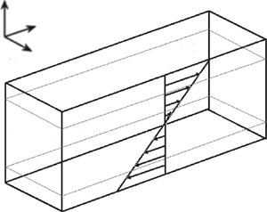
Figure 1. Flow geometry featuring a sampling domain of size  $L_x^* \times (L_y^*-2\delta _y^*) \times L_z^*$ for simulation of uniform shear turbulence.
Given the rather severe nature of the approximations made in the QL models, such as S3T and RNL, it is somehow natural to expect that their capability would be limited in certain aspects of the dynamics. However, it is important to point out that, despite the severeness of the approximation, the QL models very well capture the key dynamics of the coherent structures (i.e. self-sustaining process) with a degree of freedom much smaller than that of DNS. This suggests that a considerable amount of the turbulence spectrum may well be epiphenomena inessential to the underlying dynamics, thereby offering a new opportunity towards the development of a quantitatively more reliable low-dimensional description of turbulent flows. In this respect, gaining the fundamental understanding of such QL models should be the ideal starting point to achieve such a goal. For example, the QL models can well be improved by incorporating more nonlinearity in a minimal manner (e.g. a smart utilisation of GQL; Marston et al. Reference Marston, Chini and Tobias2016; Tobias & Marston Reference Tobias and Marston2017). Or it can be combined with an ad-hoc model to deal with the ignored nonlinear energy transport (e.g. eddy viscosity model in Hwang & Eckhardt Reference Hwang and Eckhardt2020) to keep the small degree of freedom of the QL models.
As the first step to achieve this goal, the present study aims to explore spectral energy transfer of the aformentioned QL model in order to gain the fundamental understanding of its precise modelling capability. For the purpose of bypassing the difficulty arising from the existence of multiple integral length scales in typical high-Reynolds-number wall-bounded turbulent flows, here we consider uniform shear turbulence where only single integral length scale is retained by prescribing the size of the computational domain. Furthermore, uniform shear turbulence has been understood to have a self-sustaining process fairly similar to the one in wall-bounded turbulence (Sekimoto, Dong & Jiménez Reference Sekimoto, Dong and Jiménez2016; Yang, Willis & Hwang Reference Yang, Willis and Hwang2018). This feature will therefore enable us to fully examine the capability of the QL model for the description of the flow with a self-sustaining process at a single integral length scale and the resulting energy cascade, before studying the flows with multiple integral length scales.
The paper is organized as follows. The QL model is introduced in § 2, where its spectral energy budget is formulated. In § 3 the statistics and spectra of the QL model for uniform shear turbulence are compared to DNS. The energy-budget and pressure-strain spectra are also presented here with a further analysis to explain the statistical features of the QL model. The paper concludes in § 4 with some remarks towards the improvement of the QL model analysed in the present study.
2. Problem formulation
2.1. Quasilinear approximation
We consider a turbulent flow under a uniform mean shear where the density and kinematic viscosity of the fluid are given by  $\rho$ and
  $\nu$, respectively. The time is denoted by
  $t$ and the space is denoted by
  $\boldsymbol {x}=(x,y,z)$, with
  $x$,
$x$,  $y$ and
  $z$ being the streamwise, transverse and spanwise directions, respectively. The QL approximation in the present study is identical to the RNL (Thomas et al. Reference Thomas, Lieu, Jovanović, Farrell, Ioannou and Gayme2014, Reference Thomas, Farrell, Ioannou and Gayme2015; Farrell et al. Reference Farrell, Gayme and Ioannou2017; Pausch et al. Reference Pausch, Yang, Hwang and Eckhardt2019): the flow field is decomposed into a streamwise mean and the remaining fluctuation, the former of which is solved by considering the full nonlinear equations whereas the latter is obtained from the linearised equations around the former. The velocity is decomposed into a streamwise averaged and the remaining component, i.e.
 \begin{equation} \boldsymbol{u}=\boldsymbol{U}_m+\boldsymbol{u}_r \end{equation}
with  $\boldsymbol {U}_m=\langle \boldsymbol {u}\rangle _x$, where
  $\langle \cdot \rangle _x$ indicates the streamwise average. Following Pausch et al. (Reference Pausch, Yang, Hwang and Eckhardt2019) we now introduce two projection operators which can decompose any flow variables into the streamwise-averaged part and the remaining one. The projection operators are defined as
 \begin{equation} \mathcal{P}_m[\boldsymbol{u}]\equiv\langle\boldsymbol{u}\rangle_x=\boldsymbol{U}_m,\quad \mathcal{P}_r[\boldsymbol{u}]\equiv\boldsymbol{u}-\langle\boldsymbol{u}\rangle_x=\boldsymbol{u}_r. \end{equation}
By the definition, the two projection operators satisfy the following properties:
 \begin{gather} \mathcal{P}_m[\cdot]+\mathcal{P}_r[\cdot]=\mathcal{I}[\cdot], \end{gather}
 \begin{gather} \mathcal{P}_m[\mathcal{P}_m[\cdot]]=\mathcal{P}_m[\cdot],\quad \mathcal{P}_r[\mathcal{P}_r[\cdot]]=\mathcal{P}_r[\cdot], \end{gather}
 \begin{gather} \mathcal{P}_m[\mathcal{P}_r[\cdot]]=\mathcal{P}_r[\mathcal{P}_m[\cdot]] =\boldsymbol{0}. \end{gather}
Here  $\mathcal {I}[\cdot ]$ is the identity operator. Also, for the particular projections defined in (2.2a,b), they satisfy another useful property:
 \begin{equation} \mathcal{P}_i[\mathcal{P}_m[\cdot]\ \mathcal{P}_j[\cdot]]=\mathcal{P}_m[\cdot]\ \mathcal{P}_i[\mathcal{P}_j[\cdot]] \end{equation}
for  $i,j=m,r$. Finally, we note that the projection operators are linear, implying that their application to linear terms does not yield any change in their original form.
Using the definition and the properties listed in (2.2a,b) and (2.3), the Navier–Stokes equations are first projected onto the  $\mathcal {P}_m$ and
  $\mathcal {P}_r$ subspaces. The subsequent linearisation of the equations for
  $\boldsymbol {u}_r$ about
  $\boldsymbol {U}_m$ leads to the QL system of interest in the present study, i.e.
 \begin{equation} \frac{\partial \boldsymbol{U}_m}{\partial t} + (\boldsymbol{U}_{m} \boldsymbol{\cdot} \boldsymbol{\nabla}_{yz}) \boldsymbol{U}_{m} =-\frac{1}{\rho}\boldsymbol{\nabla}_{yz} P_m + \nu \boldsymbol{\nabla}_{yz}^2 \boldsymbol{U}_m -\mathcal{P}_m\left[\left(\boldsymbol{u}_{r} \boldsymbol{\cdot} \boldsymbol{\nabla}\right)\boldsymbol{u}_{r}\right] \end{equation}
with  $\boldsymbol {\nabla }_{yz}\equiv (0,\partial _y,\partial _z)$, and
 \begin{equation} \frac{\partial \boldsymbol{u}_r}{\partial t} + \left(\boldsymbol{U}_m \boldsymbol{\cdot} \boldsymbol{\nabla}\right) \boldsymbol{u}_r + \left(\boldsymbol{u}_r \boldsymbol{\cdot} \boldsymbol{\nabla}\right) \boldsymbol{U}_m =-\frac{1}{\rho}\boldsymbol{\nabla} p_r + \nu \nabla^2 \boldsymbol{u}_r, \end{equation}
where  $P_m$ and
  $p_r$ are defined to enforce
  $\boldsymbol {\nabla }_{yz} \boldsymbol {\cdot } \boldsymbol {U}_m=0$ and
  $\boldsymbol {\nabla } \boldsymbol {\cdot } \boldsymbol {u}_r=0$, respectively, with
  $p=P_m+p_r$. We note that, as discussed in Pausch et al. (Reference Pausch, Yang, Hwang and Eckhardt2019), the QL approximation made here does not damage the energy-conservative nature of the nonlinear terms in the Navier–Stokes equations (see also § 2.3).
The QL approximation introduced here is evidently one of the many possible. However, this particular QL approximation offers a minimal way to generate self-sustaining turbulence in parallel shear flow without an instability of mean flow, because (2.4a) cannot generate a turbulent solution without its last term on the right-hand side. Furthermore, (2.4) also provides a sound physical description for the so-called ‘self-sustaining process’ (e.g. Waleffe Reference Waleffe1997), the two-way interaction between ‘streamwise elongated’ velocity structures (streaks/rolls) and ‘streamwise wavy’ structures (waves). Indeed, (2.4a) is designed to describe the dynamics of streaks and rolls, while (2.4b) depicts that of waves originating from an instability of (2.4a). This particular QL approximation has therefore been of primary interest in many previous studies (e.g. Farrell & Ioannou Reference Farrell and Ioannou2012; Thomas et al. Reference Thomas, Lieu, Jovanović, Farrell, Ioannou and Gayme2014; Farrell et al. Reference Farrell, Ioannou, Jiménez, Constantinou, Lozano-Durán and Nikolaidis2016; Pausch et al. Reference Pausch, Yang, Hwang and Eckhardt2019). In the present study we shall also focus on this particular QL approximation, and we will leave the study of more generalised variants (e.g. Marston et al. Reference Marston, Chini and Tobias2016) for future work.
Lastly, it should be pointed out that the QL approximation needs to be distinguished from ‘truncation’ for the resolution of a given simulation. The truncation does not simply provide enough degrees of freedom for the given system, while keeping the nonlinear self-interaction term, such as the one with  $\mathcal {P}_r$ in (2.8b). For this reason, the resulting low-dimensional system obtained by the truncation is contaminated by the related numerical error. In contrast, the QL approximation linearises the equations for the motions of less interest. By doing so, a degree of freedom smaller than that of DNS is spontaneously obtained, resulting in a resolution-independent low-dimensional description of the given flow (see also § 3 for this feature). In this respect, it is finally worth mentioning some previous studies which utilised a ‘minimal streamwise unit’ (e.g. Toh & Itano Reference Toh and Itano2005; Abe, Antonia & Toh Reference Abe, Antonia and Toh2018). The minimal streamwise unit approach is neither a truncation nor a QL approximation. It utilises the full resolution with a unrealistically short streamwise domain for its own purpose, while keeping the nonlinearity.
2.2. Reynolds decomposition
To analyse the turbulence statistics of the given QL system and the original system, here we start by considering the Reynolds decomposition of the velocity  $\boldsymbol {u}=(u,v,w)$ with the full Navier–Stokes equations
 \begin{equation} \boldsymbol{u}=\boldsymbol{U}+\boldsymbol{u}', \end{equation}
in which  $\boldsymbol {U}\,(\equiv \langle \boldsymbol {u} \rangle _{x,z,t})=(U(y),0,0)$ is the mean velocity with
  $\langle \cdot \rangle _{x,z,t}$ being an average in
  $t$-,
$t$-,  $x$- and
  $z$-directions. The equation for the mean streamwise velocity is then given by
 \begin{equation} \nu\frac{\mathrm{d}U}{\mathrm{d}y}-\langle u' v'\rangle_{x,z,t}=\frac{\tau_0}{\rho}, \end{equation}
where  $\tau _0$ is the applied total shear stress and
  $\langle u' v'\rangle _{x,z,t}$ the Reynolds shear stress per unit density. The equations for turbulent fluctuations are obtained by taking the remaining part of the momentum equations:
 \begin{equation} \frac{\partial \boldsymbol{u}'}{\partial t} + (\boldsymbol{U} \boldsymbol{\cdot} \boldsymbol{\nabla})\, \boldsymbol{u}' + (\boldsymbol{u}' \boldsymbol{\cdot} \boldsymbol{\nabla}) \,\boldsymbol{U} =-\frac{1}{\rho}\boldsymbol{\nabla} p' + \nu \nabla^2 \boldsymbol{u}'-(\boldsymbol{u}' \boldsymbol{\cdot} \boldsymbol{\nabla})\,\boldsymbol{u}'. \end{equation}
Here, we note that the Reynolds shear-stress term in (2.6a) does not appear in (2.6b) because it is spatially uniform in uniform shear turbulence.
For the QL approximation to (2.6b), the turbulent velocity fluctuation is further decomposed into a streamwise averaged and the remaining component (2.1):
 \begin{equation} \boldsymbol{u}'=\boldsymbol{u}_m+\boldsymbol{u}_r \end{equation}
with  $\boldsymbol {u}_m=\langle \boldsymbol {u}'\rangle _x$. Using the definition and the properties listed in (2.2a,b) and (2.3), the projection of the equations for turbulent fluctuation onto the
  $\mathcal {P}_m$ and
  $\mathcal {P}_r$ subspaces leads to the momentum equations
 \begin{equation} \frac{\partial \boldsymbol{u}_m}{\partial t} + (\boldsymbol{u}_m\boldsymbol{\cdot} \boldsymbol{\nabla}_{yz}) \,\boldsymbol{U}=-\frac{1}{\rho}\boldsymbol{\nabla}_{yz} p_m + \nu \boldsymbol{\nabla}_{yz}^2 \boldsymbol{u}_m - (\boldsymbol{u}_{m} \boldsymbol{\cdot} \boldsymbol{\nabla}_{yz}) \,\boldsymbol{u}_{m}-\mathcal{P}_m\,[(\boldsymbol{u}_{r} \boldsymbol{\cdot} \boldsymbol{\nabla})\,\boldsymbol{u}_{r}] \end{equation}
with  $\boldsymbol {\nabla }_{yz}\equiv (0,\partial _y,\partial _z)$, and
 \begin{equation} \frac{\partial \boldsymbol{u}_r}{\partial t} + (\boldsymbol{U}_m \boldsymbol{\cdot} \boldsymbol{\nabla}) \,\boldsymbol{u}_r + (\boldsymbol{u}_r \boldsymbol{\cdot} \boldsymbol{\nabla}) \,\boldsymbol{U}_m =-\frac{1}{\rho}\boldsymbol{\nabla} p_r + \nu \nabla^2 \boldsymbol{u}_r-\mathcal{P}_r\,[(\boldsymbol{u}_{r} \boldsymbol{\cdot} \boldsymbol{\nabla} )\,\boldsymbol{u}_{r}], \end{equation}
where  $\boldsymbol {U}_m=\boldsymbol {U}+\boldsymbol {u}_m$, and
  $p_m$ and
  $p_r$ are defined to enforce
  $\boldsymbol {\nabla }_{yz} \boldsymbol {\cdot } \boldsymbol {u}_m=0$ and
  $\boldsymbol {\nabla } \boldsymbol {\cdot } \boldsymbol {u}_r=0$, respectively, with
  $p'=p_m+p_r$. For the QL approximation to be examined in the present study, the self-interaction term
  $\mathcal {P}_r\left [\left (\boldsymbol {u}_{r} \boldsymbol {\cdot } \boldsymbol {\nabla } \right )\boldsymbol {u}_{r}\right ]$ in (2.8b) will be ignored. We also note that the sum of the equation obtained by differentiating (2.6a) in the
  $y$-direction, (2.8a) and (2.8b) without its last self-interaction term yields (2.4).
2.3. Spectral energetics
To study the effect of the QL approximation on the energetics of the given flow, let us first consider the mean equation in (2.6a). We note that every term in this equation is constant in uniform shear flow, enabling us to take a further average in the transverse direction. Multiplication of (2.6a) by  $\textrm {d}U/\textrm {d}y$ and its rearrangement then lead to the following equation for the mean energetics:
 \begin{equation} I-\nu\left(\frac{\textrm{d}U}{\textrm{d}y}\right)^2+\langle u' v'\rangle_{x,y,z,t}\frac{\textrm{d}U}{\textrm{d}y}=0,\quad \text{where}\ I\equiv \frac{\tau_0}{\rho}\frac{\textrm{d}U}{\textrm{d}y}. \end{equation}
Equation (2.9) suggests that the energy input to the flow originates from the applied shear stress  $\tau _0$, and it is balanced with mean dissipation (the second term) and turbulent kinetic-energy (TKE) production (the third term). Hence, the latter TKE production term becomes the source term in the TKE equation (Tennekes & Lumley Reference Tennekes and Lumley1967).
In the present study the TKE equation is considered in the streamwise/spanwise Fourier space, so that the inter-scale energy transfer can be studied. For this purpose, one-dimensional Fourier-mode decomposition for the turbulent velocity fluctuations is introduced, i.e.
 \begin{equation} u_j^{\prime}(t,r)=\int_{-\infty}^{\infty} \widehat{u_j^{\prime}}(t,k) \textrm{e}^{\mathrm{i} k r}\, \mathrm{d}k \end{equation}
for  $j=1,2,3$, where
  $\hat {\cdot }$ denotes the Fourier-transformed coefficient,
  $\left (u_1^{\prime },u_2^{\prime },u_3^{\prime }\right )=\left (u^{\prime },v^{\prime },w^{\prime }\right )$,
  $r\,(=x\ \mathrm {or}\ z)$ is the streamwise or spanwise coordinate, and
  $k\,(=k_x\ \mathrm {or}\ k_z)$ the corresponding wavenumber. We then take the Fourier transformation (2.10) to (2.6b), and multiply it by the complex conjugate of
  $\widehat {u_i'}(k)$. Since the statistics of uniform shear turbulence should be invariant under the translation in the transverse direction, taking an average in time, transverse direction and the planar direction along which the Fourier transform is not taken (denoted by
  $r^{\perp }$) yields
 \begin{align} & \underbrace{\left\langle \mathrm{Re} \left\{- \overline{\widehat{u^{\prime}}} (k)\widehat{v^{\prime}}(k) \, \frac{\mathrm{d} U}{\mathrm{d} y} \right\} \right\rangle_{r^{\perp},y,t}}_{\hat{P}\left(k \right)} +\underbrace{\left\langle - \nu \frac{\partial{\widehat{u_{i}^{\prime}}(k)} }{\partial{x_{j}} } \frac{\partial{\overline{\widehat{u_{i}^{\prime}}}(k)} }{\partial{x_{j}} } \right\rangle_{r^{\perp},y,t}}_{\hat{\varepsilon}\left(k \right)} \nonumber\\ &\qquad + \underbrace{\left\langle \mathrm{Re} \left\{- \overline{\widehat{u_{i}^{\prime}}}(k) \left(\frac{\partial }{\partial{x_{j}} } \left( \widehat{ u_{i}^{\prime}u_{j}^{\prime} }(k) -\mathcal{P}_r\left[\widehat{ u_{r,i}^{\prime}u_{r,j}^{\prime} }(k)\right] \right) \right) \right\} \right\rangle_{r^{\perp},y,t}}_{\hat{T}\left(k\right)}=0, \end{align}
where  $(x_1,x_2,x_3)=(x,y,z)$, the overbar indicates the complex conjugate and
  $\mathrm {Re} \{\, \cdot \,\}$ the real part. The terms on the right-hand side are the rate of turbulence production,
  $\hat {P}(k)$, viscous dissipation,
  $\hat {\varepsilon }(k)$, and (nonlinear) turbulent energy transport,
  $\hat {T}(k)$, at a given wavenumber, respectively. Here, we note that the term with
  $\mathcal {P}_r$ in
  $\hat {T}(k)$ appears when the last term on the right-hand side of (2.8b) is ignored, indicating that the given QL approximation directly damages turbulent energy transport. Furthermore, since
  $\int _{0}^{\infty } \hat {T}(k) \mathrm {d}k=0$, the exact statistical balance between the production and dissipation of TKE is obtained for both of the full and QL systems through (2.11), i.e.
 \begin{equation} P+\varepsilon=0, \end{equation}
where
 \begin{equation} P=2\int_{0}^{\infty} \hat{P}\left(k\right)\, \mathrm{d}k\quad \text{and}\quad \varepsilon=2\int_{0}^{\infty} \hat{\varepsilon}\left(k\right)\,\mathrm{d}k. \end{equation}
Finally,  $P=-\langle u' v'\rangle _{x,y,z,t}\,\textrm {d}U/\,\textrm {d}y$ is retrieved from (2.12b), forming a complete energy balance through the mean and fluctuation equations through (2.9) and (2.12).
Equation (2.11) can be further split into each component for the componentwise TKE budget,
 \begin{align} 0 & =\hat{P}(k)+ \underbrace{\left \langle Re \left \{ \frac{\widehat{p'} (k)}{\rho} \frac{\partial \overline{\widehat{u'}} (k)}{\partial x} \right \} \right\rangle_{r^{\perp},y,t}}_{\hat{\varPi}_x(k)}+ \underbrace{\left \langle -\nu \frac{\partial \widehat{u'} (k)}{\partial x_j} \frac{\partial \overline{\widehat{u'}} (k)}{\partial x_j} \right \rangle_{r^{\perp},y,t}}_{\hat{\varepsilon}_x(k)} \nonumber\\ &\quad \underbrace{\left\langle \mathrm{Re} \left\{- \overline{\widehat{u^{\prime}}}(k) \left(\frac{\partial }{\partial{x_{j}} } \left( \widehat{ u^{\prime}u_{j}^{\prime} }(k) -\mathcal{P}_r\left[\widehat{ u_{r}^{\prime}u_{r,j}^{\prime} }(k)\right] \right) \right)\: \right\} \right\rangle_{r^{\perp},y,t}}_{\hat{T}_x\left(k\right)}, \end{align}
 \begin{align} 0 &= \underbrace{\left \langle Re \left \{\frac{\widehat{p'} (k)}{\rho} \frac{\partial \overline{\widehat{v'}} (k)}{\partial y} \right \} \right \rangle_{r^{\perp},y,t}}_{\hat{\varPi}_y(k)} + \underbrace{\left \langle -\nu \frac{\partial \widehat{v'} (k)}{\partial x_j} \frac{\partial \overline{\widehat{v'}} (k)}{\partial x_j} \right \rangle_{r^{\perp},y,t}}_{\hat{\varepsilon}_y(k)} \nonumber\\ &\quad + \underbrace{\left\langle \mathrm{Re} \left\{- \overline{\widehat{v^{\prime}}}(k) \left(\frac{\partial }{\partial{x_{j}} } \left( \widehat{ v^{\prime}u_{j}^{\prime} }(k) -\mathcal{P}_r\left[\widehat{v_{r}^{\prime}u_{r,j}^{\prime}}(k)\right] \right) \right) \right\} \right\rangle_{r^{\perp},y,t}}_{\hat{T}_y\left(k\right)}, \end{align}
 \begin{align} 0 &=\underbrace{\left \langle Re \left \{\frac{\widehat{p'} (k)}{\rho} \frac{\partial \overline{\widehat{w'}} (k)}{\partial z} \right \} \right \rangle_{r^{\perp},y,t}}_{\hat{\varPi}_z(k)} + \underbrace{\left \langle -\nu \frac{\partial \widehat{w'} (k)}{\partial x_j} \frac{\partial \overline{\widehat{w'}} (k)}{\partial x_j} \right \rangle_{r^{\perp},y,t}}_{\hat{\varepsilon}_z(k)} \nonumber\\ &\quad + \underbrace{\left\langle \mathrm{Re} \left\{- \overline{\widehat{w'}} (k) \left(\frac{\partial }{\partial{x_{j}} } \left( \widehat{ w^{\prime}u_{j}^{\prime} }(k) -\mathcal{P}_r\left[\widehat{ w_{r}^{\prime}u_{r,j}^{\prime} }(k)\right] \right) \right)\: \right\} \right\rangle_{r^{\perp},y,t}}_{\hat{T}_z(k)}, \end{align}
where  $\hat {\varPi }_x$,
  $\hat {\varPi }_y$ and
  $\hat {\varPi }_z$ are one-dimensional spectra of the streamwise, wall-normal and spanwise components of pressure strain, respectively. We note that the pressure-strain terms do not appear in (2.11) because the continuity equation gives
 \begin{equation} \hat{\varPi}_x(k)+\hat{\varPi}_y(k)+\hat{\varPi}_z(k)=0. \end{equation}
The relation above is of crucial importance, as it indicates that the pressure-strain terms would play an important role in the TKE distribution to the individual velocity components through continuity. It is evident that the turbulent production only takes place in (2.13a), but not in (2.13b) nor in (2.13c). In wall-bounded turbulent flows the pressure-strain terms have indeed been found to play the primary role in the distribution of the TKE produced at the streamwise component to the others (Cho, Hwang & Choi Reference Cho, Hwang and Choi2018; Lee & Moser Reference Lee and Moser2019). In particular, if the isotropy of fluid motions at dissipation scale is assumed (Kolmogorov Reference Kolmogorov1941), the pressure-strain terms must mediate the conversion of highly anisotropic large scale into isotropic small scale during energy cascade.
2.4. Numerical simulations
The equations in the present study are made dimensionless with the shear stress imposed  $\tau _0$ and the kinematic viscosity
  $\nu$. Using the resulting velocity and length scales respectively given by
  $u_{\tau }=\sqrt {\tau _0/\rho }$ and
  $\eta =\nu /u_{\tau }$, the mean-momentum equation is obtained as
 \begin{equation} \frac{\mathrm{d}U^*}{\mathrm{d}y^*}-{\langle {u'}^* {v'}^*\rangle_{x,z,t}}=1, \end{equation}
and the fluctuations equations are
 \begin{equation} \frac{\partial {\boldsymbol{u}'}^*}{\partial t^*} + (\boldsymbol{U}^* \boldsymbol{\cdot} \boldsymbol{\nabla}^*) \,{\boldsymbol{u}'}^* + ({\boldsymbol{u}'}^* \boldsymbol{\cdot} \boldsymbol{\nabla}^*) \,\boldsymbol{U}^* =-\boldsymbol{\nabla}^* {p'}^* + {\boldsymbol{\nabla}^*}^2 {\boldsymbol{u}'}^*-({\boldsymbol{u}'}^* \boldsymbol{\cdot} \boldsymbol{\nabla}^*)\,{\boldsymbol{u}'}^*, \end{equation}
where the superscript  $*$ denotes the resulting dimensionless variables. We note that the viscous terms in (2.15a) and (2.15b) turn out to be order of unity, implying that
  $u_{\tau }$ and
  $\eta$ correspond to the Kolmogorov velocity and length scales, respectively (for a detailed discussion, see also Yang et al. Reference Yang, Willis and Hwang2018). The velocity and the length scales of the largest eddies admitted are given by
  $\Delta U^*=L_z^*$ and
  $L_z^*$ in the Kolmogorov units, where
  $\Delta U$ would indicate the difference in the mean velocity over the characteristic large-eddy size
  $L_z$ in the transverse direction. From this, it is not difficult to realize that
  $L_z^*$ is a Reynolds number
  $Re_{\tau ,L_z}(=L_z^*)\equiv u_{\tau } L_z/\nu$ which characterizes the separation between the largest and smallest length scales in the flow.
Direct numerical simulations and simulations of the QL model for uniform shear turbulence are carried out following the recent approach of Yang et al. (Reference Yang, Willis and Hwang2018). Figure 1 shows a schematic diagram explaining how uniform shear flow is simulated in the present study. A simulation is first set up for plane Couette flow where the two parallel sliding walls with the velocity  ${\pm }U_0$ are located at
  $y={\pm }L_y/2$, respectively. The spanwise domain of the simulation is then designed to be highly restricted, such that the size of the largest eddies in the bulk region is determined by the spanwise domain size
  $L_z$. This approach is similar to the minimal-flow-unit approach used to isolate the near-wall dynamics in pressure-driven channel flow (Jiménez & Moin Reference Jiménez and Moin1991; Hwang Reference Hwang2013). However, in this case where the laminar base flow is uniform shear, the equations of motion are exactly identical to (2.6). As such, the bulk region of the flow in effect simulates a uniform shear flow (Yang et al. Reference Yang, Willis and Hwang2018) – note that the influence of the near-wall structures should remain to be confined only in the near-wall region, the relevant thickness of which would be at best
  $O(L_z)$. With this simulation set-up, the statistics of uniform shear turbulence can now be sampled from the bulk region of the flow where the effect of the two solid walls becomes negligible (i.e.
  $y\in [-L_y/2+\delta _y,L_y/2-\delta _y]$ in figure 1; see also figure 2 where the bulk region indeed exhibits uniform shear and velocity fluctuations). Finally, the simulations with a highly restricted spanwise domain can contain a non-physical box-size-related two-dimensional motion resolved by zero spanwise wavenumber, especially if the streamwise domain size is very long (Hwang Reference Hwang2013). This motion is eliminated using the filtering approach proposed by Hwang (Reference Hwang2013).

Figure 2. First- and second-order turbulence statistics (L-DNS) for  $y^*\in [0,L_y^*/2]$. Here, the sampling domain is delimited by the solid vertical line separating the bulk from the near-wall region.
  $(a)$
$(a)$ $U^*(y^*)$.
  $(b)$
$(b)$ $u_{rms}^*$,
  $v_{rms}^*$ and
  $w_{rms}^*$.
The numerical solver used in this investigation is Diablo (Bewley Reference Bewley2014), the use of which has been verified by a number of previous studies (e.g. Yang et al. Reference Yang, Willis and Hwang2018; Doohan, Willis & Hwang Reference Doohan, Willis and Hwang2019). In this solver the streamwise and spanwise directions are discretized using Fourier series with  $2/3$ rule for dealiasing, and the wall-normal direction is discretized using the second-order central difference. The time integration is conducted semi-implicitly based on the fractional-step method (Kim & Moin Reference Kim and Moin1985). All the viscous terms are implicitly advanced with a second-order Crank–Nicolson method, while the rest of the nonlinear advection terms are explicitly integrated with a low-storage third-order Runge–Kutta method.
Table 1 summarizes the parameters for the simulations performed in this study. Two sets of Reynolds numbers are considered:  $Re_{\tau ,L_z} \simeq 136$ and
  $514$ based on the direct numerical simulation results (see the cases of L-DNS and H-DNS in table 1). The domains size of the low-Reynolds-number case (L) is similar to that of the typical minimal unit for near-wall turbulence (Jiménez & Moin Reference Jiménez and Moin1991), where the dynamics of the large eddies is well described by the so-called self-sustaining process (Hamilton et al. Reference Hamilton, Kim and Waleffe1995; Yang et al. Reference Yang, Willis and Hwang2018). In this case, due to the low Reynolds number considered, the simulation exhibits very little energy cascade for dissipation. On the other hand, the high-Reynolds number case (H) is set to contain a non-negligible extent of energy cascade for turbulent dissipation, so that the effect of QL approximation on the cascade can be examined. For each Reynolds-number case, the number of streamwise Fourier modes used in the QL approximation is also varied from the minimal (
 $N_{x,F}=1$, where
  $N_{x,F}$ is the number of positive-wavenumber streamwise Fourier modes) to the maximal number, the latter of which corresponds to that of DNS. Finally, the aspect ratio of the streamwise domain to the spanwise one is chosen to be
  $L_x/L_z=3$, in line with the previous investigation of Sekimoto et al. (Reference Sekimoto, Dong and Jiménez2016).
Table 1. Simulation parameters in the present study. We denote by  $L_x^*$,
  $L_y^*$ and
  $L_z^*$ the domain size in the
  $x$-,
$x$-,  $y$- and
  $z$ directions in the Kolmogorov unit, respectively. Here,
  $Re=U_0 L_y/(2\nu )$,
  $Re_{\tau ,Lz}=L_z^*$ and
  $Re_{\lambda }$ is the Reynolds number based on the Taylor microscale. The grid spacings in the
  $x$- and
  $z$-directions are
  $\Delta _x^*$ and
  $\Delta _z^*$ (after aliasing). The number of the positive-wavenumber streamwise Fourier modes is denoted by
  $N_{x,F}$, and the number of streamwise grid points is given by
  $N_x=2N_{x,F}+1$. The number of grid points in the
  $y$- and
  $z$-directions are denoted by
  $N_y$ and
  $N_z$, respectively.

3. Results and discussion
3.1. Turbulence statistics and spectra
We first consider the set of DNS and the corresponding QL counterparts for the two Reynolds numbers, while maintaining the same  $Re$ (see table 1). For both of the Reynolds numbers, the QL model exhibits elevation of
  $Re_{\tau ,L_z}$ irrespective of the number of streamwise Fourier modes
  $N_{x,F}$, indicating that
  $\tau _0$ applied through the Couette flow is increased by applying the QL approximation. From (2.9), this implies that the energy input given to the flow is increased by the QL approximation, also explaining the increased
  $Re_{\lambda }$ for all the simulations of the QL model. If the flow in the QL model is more turbulent, the contribution of the Reynolds shear-stress term in (2.15a) should also increase. This is indeed seen in the Reynolds shear stress of the QL model, as shown in table 2. Consequently,
  $\textrm {d}U^*/\textrm {d}y^*$ is decreased from the mean equation (2.15a).
Table 2. One-point turbulence statistics. Here,  $S^*(\equiv \textrm {d}U/\textrm {d}y q^2/|\varepsilon |$) is the Corrsin shear parameter (Corrsin Reference Corrsin1958), where
  $S=\textrm {d}U/\textrm {d}y$,
  $q^2={u^2_{rms}}+{v^2_{rms}}+{w^2_{rms}}$ and
  $\varepsilon$ is given in (2.12a).

The QL model is also found to generate more anisotropic velocity fluctuations. In particular,  $u_{rms}^*$ and
  $v_{rms}^*$ are increased in the QL model regardless of the
  $N_{x,F}$ considered, whereas
  $w_{rms}^*$ is decreased (see table 2). This behaviour is a little different from that observed in wall-bounded shear flows (e.g. Thomas et al. Reference Thomas, Lieu, Jovanović, Farrell, Ioannou and Gayme2014; Farrell et al. Reference Farrell, Ioannou, Jiménez, Constantinou, Lozano-Durán and Nikolaidis2016), where only
  $u_{rms}^*$ is increased by the QL approximation while the others are decreased. While this points to some non-negligible differences between uniform shear and wall-bounded shear flows, the present QL model also generates a turbulent fluctuation more skewed to the streamwise component (see also § 3.3 for a further discussion). Finally, the QL model exhibits one-point turbulence statistics well converged for
  $N_{x,F}\geq 5$ (see table 2). This implies that only a reasonably small number of the streamwise Fourier modes are active in the QL model, consistent with the previous observations made in wall-bounded flows (e.g. Thomas et al. Reference Thomas, Lieu, Jovanović, Farrell, Ioannou and Gayme2014, Reference Thomas, Farrell, Ioannou and Gayme2015; Farrell et al. Reference Farrell, Ioannou, Jiménez, Constantinou, Lozano-Durán and Nikolaidis2016; Tobias & Marston Reference Tobias and Marston2017) (see also figure 5).
Figure 3 compares premultiplied spanwise wavenumber spectra of Reynolds stress of DNS (H-DNS) with those of the QL simulation with full streamwise resolution (H-QL-FULL) in the high-Reynolds-number case. The spectra of the low-Reynolds-number case are found to show qualitative similitude to the high-Reynolds-number ones. Therefore, they will not be presented hereafter to avoid any unnecessary repetitions. We note that the area below in each premultiplied spectrum approximately represents the energy contained by each component of the Reynolds stress, showing consistency with the one-point statistics reported in table 2 (note that the discrete spectra shown in figure 3 do not include the energy contained by  $k_z=0$ mode). It appears that the QL model shows an increased spectral energy of all the Reynolds stress components at large scale (
 $k_zL_z>10$). However, at high spanwise wavenumbers, the spectra of the QL model fall off more rapidly than those of DNS.

Figure 3. Premultiplied spanwise wavenumber spectra of Reynolds stresses of DNS (H-DNS) and the QL model (H-QL-FULL).  $(a)$
$(a)$ $k_zL_z\varPhi_{uu}^*(k_zL_z)$.
  $(b)$
$(b)$ $k_zL_z\varPhi_{vv}^*(k_zL_z)$.
  $(c)$
$(c)$ $k_zL_z\varPhi_{ww}^*(k_zL_z)$.
  $(d)$
$(d)$ $-k_zL_z\varPhi_{uv}^*(k_zL_z)$.
Figure 4 shows the same spanwise wavenumber spectra of DNS and the QL model in logarithmic units. All the Reynolds normal-stress spectra of DNS (figure 4 $a$–
$a$– $c$) exhibit a relatively short range of the typical inertial subrange spectra, featured with the
  $-5/3$ law, up to
  $k_zL_z \approx 50$ (Kolmogorov Reference Kolmogorov1941). The Reynolds shear-stress spectra also follows the
  $-7/3$ law (solid lines in figure 4
 $d$) (Lumley Reference Lumley1967; Saddoughi & Veeravalli Reference Saddoughi and Veeravalli1994). For
  $k_zL_z>50$, the spectra of DNS show that small-scale turbulence is close to isotropic (Kolmogorov Reference Kolmogorov1941); for example, at
  $k_zL_z=10^2$,
  $\varPhi_{uu}^*\simeq 10^{-2}$,
  $\varPhi_{vv}^* \simeq 10^{-2}$,
  $\varPhi_{ww}^* \simeq 10^{-3}$ and
  $-\varPhi_{uv}^* \simeq 10^{-4}$. This is in sharp contrast to the spectra of the QL model. First of all, regardless of the number of streamwise Fourier modes (
 $N_{x,F}$) considered, all the Reynolds normal-stress spectra of the QL model decay faster than those of DNS with
  $k_z$ (figure 4
 $a$–
$a$– $c$). In particular, the decay of the transverse and spanwise components of the spectra (figure 4
 $b$,
$b$, $c$) appears to be much more drastic than that of the streamwise counterpart (figure 4
 $a$). While it is unclear whether the spectra of the Reynolds normal stresses from the QL model would still obey the
  $-5/3$ law due to the relatively low Reynolds numbers considered in the present study, the turbulence at small scale is evidently no more isotropic. Indeed, for the QL model with sufficiently large streamwise resolution (
 $N_{x,F}>16$),
  $\varPhi_{uu}^*\simeq 10^{-3}$,
  $\varPhi_{vv}^* \simeq 10^{-4}$,
  $\varPhi_{ww}^* \simeq 10^{-5}$ and
  $-\varPhi_{uv}^* \simeq 10^{-4}$. This suggests that the QL approximation destroys the main statistical features of energy cascade and dissipation in a turbulent flow, although it still allows for nonlinear energy transport in the spanwise wavenumber space via the self-interacting nonlinear term in (2.8a) (i.e. the third term on the right-hand side).

Figure 4. Spanwise wavenumber spectra of Reynolds stresses of DNS (H-DNS) and the QL model for several different streamwise resolutions (see table 1).  $(a)$
$(a)$ $\varPhi_{uu}^*(k_zL_z)$.
  $(b)$
$(b)$ $\varPhi_{vv}^*(k_zL_z)$.
  $(c)$
$(c)$ $\varPhi_{ww}^*(k_zL_z)$.
  $(d)$
$(d)$ $-\varPhi_{uv}^*(k_zL_z)$.
The premultiplied streamwise wavenumber spectra of Reynolds stresses are shown in figure 5 for DNS (H-DNS) and the QL model with full streamwise resolution (H-QL-FULL). As reported in previous studies (Thomas et al. Reference Thomas, Lieu, Jovanović, Farrell, Ioannou and Gayme2014, Reference Thomas, Farrell, Ioannou and Gayme2015; Farrell et al. Reference Farrell, Ioannou, Jiménez, Constantinou, Lozano-Durán and Nikolaidis2016; Tobias & Marston Reference Tobias and Marston2017), the energy in the spectra is retained within a highly limited range of streamwise wavenumbers ( $k_xL_z \lesssim 11$ in figure 5). We note that the primary role of the self-interacting nonlinear term in the present QL approximation (i.e. the last term in (2.8b)) lies in the coupling between streamwise Fourier modes of (2.8b). Therefore, this is a direct consequence of the removal of the related turbulent energy transport (i.e. energy cascade) in the streamwise wavenumber space, as will be directly shown in § 3.2. Lastly, the spectral intensity of the QL model is found to be much higher than that of DNS. This feature also appears in previous studies (e.g. Thomas et al. Reference Thomas, Lieu, Jovanović, Farrell, Ioannou and Gayme2014; Farrell et al. Reference Farrell, Ioannou, Jiménez, Constantinou, Lozano-Durán and Nikolaidis2016; Marston et al. Reference Marston, Chini and Tobias2016; Tobias & Marston Reference Tobias and Marston2017). In particular, in Zonal jets, Marston et al. (Reference Marston, Chini and Tobias2016) pointed out that this is due to the absence of ‘eddy scattering’. Indeed, a reason for the elevation of spectral energy intensity would be the absence of the streamwise energy cascade in the QL model: the TKE in the QL model must be retained only within a small range of streamwise wavenumbers, as it maintains roughly the same level of TKE as DNS (see table 2). However, it should also be pointed out that the mean and the fluctuations are mutually connected in a way that when the dynamics is perturbed by the removal of some nonlinearity, the turbulence adjusts to a new statistical equilibrium. Therefore, care also needs to be taken for interpretation of this feature.

Figure 5. Premultiplied streamwise wavenumber spectra of Reynolds stresses.  $(a)$
$(a)$ $k_xL_z\varPhi_{uu}^*(k_xL_z)$.
  $(b)$
$(b)$ $k_xL_z\varPhi_{vv}^*(k_xL_z)$.
  $(c)$
$(c)$ $k_xL_z\varPhi_{ww}^*(k_xL_z)$.
  $(d)$
$(d)$ $-k_xL_z\varPhi_{uv}^*(k_xL_z)$.
Finally, the premultiplied streamwise and spanwise wavenumber spectra of the pressure are shown in figure 6 for the DNS and QL model with full streamwise resolution. The streamwise spectra show the disruption of the nonlinear transport in that direction when the QL model is applied. In this case, the spanwise spectra of the QL model are below those of the DNS for the whole spanwise domain, featuring a quick decay as previously found for the spectra of the Reynolds stresses.

Figure 6. Premultiplied streamwise  $(a)$ and spanwise
  $(b)$ wavenumber spectra of the pressure for H-DNS and H-QL-FULL.
  $(a)$
$(a)$ $k_z L_z \varPhi_{pp}^*(k_z L_z)$.
  $(b)$
$(b)$ $k_x L_z \varPhi_{pp}^*(k_x L_z)$.
3.2. Spectral energy transfer
Now we study the spectral energy transfer in both DNS and the QL model. Given the perfect balance between production and dissipation in both DNS and QL simulations shown in (2.12), the spectral energy density of each term in (2.11) is expected to be dependent of the rate of production of each simulation, yielding a difficulty to make a fair comparison of one case to another in regards to how the TKE produced by mean shear is distributed. For this reason, here we consider the spectral energy budget per unit mean shear instead, i.e.  $\hat {P}(k)/(\textrm {d}U/\textrm {d}y)$,
  $\hat {T}(k)/(\textrm {d}U/\textrm {d}y)$ and
  $\hat {\varepsilon }(k)/(\textrm {d}U/\textrm {d}y)$. By doing so, the inner-scaled turbulence production per unit mean shear is now controlled to be
  $P^*/(\textrm {d}U^*/\textrm {d}y^*)=0.99$ for all the simulations carried out at high Reynolds number (see table 2).
The premultiplied one-dimensional spanwise wavenumber spectra of the production, turbulent transport and dissipation per unit mean shear from DNS and the QL model are plotted in figure 7. At first glance, all the plots appear to show a qualitatively similar behaviour: production takes place at large scales ( $k_zL_z\lesssim 20$) and this energy appears to be transferred almost equally to turbulent transport and viscous dissipation, the latter phenomenon of which is presumably due to the still relatively low Reynolds number considered in the present study. At small scales (
 $k_zL_z \gtrsim 50$), the production becomes negligible and the other two terms balance each other with the turbulent transport term being positive. The spectra of the H-QL-NX4 case (
 $N_{x,F}=1$) also appear to agree reasonably well with those of the H-QL-FULL case (
 $N_{x,F}=54$) – in fact, the spanwise energy-budget spectra of the QL model remain almost identical as long as
  $N_{x,F}\geq 5$ (see figure 7
 $b{,}c$), consistent with the turbulence statistics reported in table 2.

Figure 7. Premultiplied streamwise wavenumber spectra of energy budget per unit mean shear:  $(a)$ H-DNS;
  $(b)$ H-QL-FULL;
  $(c)$ H-QL-NX4;
  $(d)$ H-QL-NX16.
Closer scrutiny of the data, however, reveals that there are also subtle but important differences between the spectra of DNS and the QL model. In particular, the turbulent transport spectra of DNS span a wider range of spanwise wavenumber than those of the QL model. Indeed, the turbulent transport spectra of H-DNS reach zero at  $k_zL_z\simeq 200$ (figure 7
 $a$), whereas those of H-QL-FULL do the same only at
  $k_z L_z \simeq 100$ (figure 7
 $b$). This is consistent with the Reynolds stress spectra in figure 4, where the spectral intensities at high spanwise wavenumber of the QL model are shown to be considerably smaller than those of DNS. For the same reason, the dissipation spectra of DNS also span a wider range of spanwise wavenumber than those of the QL model. Here, it should be stressed that all these observations on turbulent transport and dissipation spectra are not due to different production of the QL model. In fact, the QL model yields production larger than DNS as the application of the QL approximation has been found to elevate
  $\tau _0$ for a fixed
  $Re$ (see (2.9) and table 2). In DNS this would rather have increased the wavenumber range of turbulent transport spectra.
The premultiplied streamwise wavenumber spectra of the energy budget per unit mean shear are shown in figure 8. While the spectra of DNS show the typical features of energy cascade and turbulent dissipation observed in figure 7 (figure 8 $a$), the QL model does not develop such features even with the streamwise resolution used in DNS (figure 8
 $b$). In particular, both turbulent transport and dissipation spectra are highly localised within the wavenumber space where turbulence production is active
  $k_xL_z \lesssim 1$ (figure 8
 $b$), explaining why the localisation of the streamwise wavenumber spectra of Reynolds stresses for
  $k_xL_z \lesssim 1$ in figure 5. Given the linear nature of (2.8b), it is not surprising to see the significantly damaged energy cascade in the streamwise wavenumber space. However, it should also be pointed out that there is still a non-negligible number of wavenumbers actively involved in the spectral TKE balance; for example, in the case of H-QL-FULL, there are still approximately five streamwise Fourier modes highly active, and they form the spectral TKE balance in the streamwise wavenumber space. Furthermore, the nonlinear turbulent transport is not completely inactive in the streamwise wavenumber space.

Figure 8. Premultiplied streamwise wavenumber spectra of energy budget per unit mean shear:  $(a)$ H-DNS;
  $(b)$ H-QL-FULL;
  $(c)$ H-QL-NX16;
  $(d)$ H-QL-NX48.
To understand these features, we examine the spectral energy budget of (2.8b). We take the streamwise Fourier transform to (2.8b) and subsequently multiply it by the complex conjugate of  $\hat {u}_{r,i}$. Taking average in time and the transverse and spanwise directions gives
 \begin{align} & \underbrace{\left\langle \mathrm{Re} \left\{- \bar{\hat{u}}_{r,i} (k_x)\hat{u}_{r,j}(k_x) \, \frac{\partial U_{m,i}}{\partial x_{j}} \right\} \right\rangle_{y,z,t}}_{\hat{P}_r(k_x)} + \underbrace{\left\langle - \nu \frac{\partial{\bar{\hat{u}}_{r,i}(k_x)} }{\partial{x_{j}} } \frac{\partial{\hat{u}_{r,i}(k_x)} }{\partial{x_{j}} } \, \right\rangle_{y,z,t}}_{\hat{\varepsilon}_r(k_x)}\nonumber\\ &\qquad + \underbrace{\left\langle \mathrm{Re} \left\{- \bar{\hat{u}}_{r,i}(k_x) \left(\frac{\partial }{\partial{x_{j}} } \left(\mathcal{P}_r\left[\widehat{ u_{r,i} u_{r,j} }(k_x)\right] \right) \right) \right\} \right\rangle_{y,z,t}}_{\hat{T}_r(k_x)}=0, \end{align}
with  $\partial /\partial x_1=\mathrm {i}k_x$. Here,
  $\hat {P}_r(k_x)$ is now the production by the interaction of
  $\hat {u}_{r,i}$ with transverse and spanwise mean shear
  $U_{m,i}\,(=U_i+u_{m,i})$,
  $\hat {\varepsilon }_r(k_x)$ the dissipation and
  $\hat {T}_r(k_x)$ the nonlinear transport through the self-interaction of
  $\hat {u}_{r,i}$. We note that, given the velocity decomposition defined in (2.5) and (2.7),
  $\widehat {u^{\prime }}_{i}(k_x)=\hat {u}_{r,i}(k_x)$ when
  $k_x\ne 0$. Furthermore, the QL approximation ignores the nonlinear transport term in (3.1). This implies that the energy of
  $\hat {u}_{r,i}(k_x)$ in the QL model is determined, such that
 \begin{equation} \hat{P}_r(k_x)+\hat{\varepsilon}_r(k_x)=0. \end{equation}
When  $k_x\ne 0$,
  $\hat {\varepsilon }_r(k_x)=\hat {\varepsilon }(k_x)$. Also,
  $\hat {P}_r(k_x)$ can further be decomposed as
 \begin{equation} \hat{P}_r(k_x)=\hat{P}(k_x)+\left\langle \mathrm{Re} \left\{- \bar{\hat{u}}_{r,i} (k_x)\hat{u}_{r,j}(k_x) \, \frac{\partial u_{m,i}}{\partial x_{j}} \right\} \right\rangle_{y,z,t}, \end{equation}
indicating that the turbulent transport defined in (2.11) should take the following form:
 \begin{equation} \hat{T}(k_x)=\left\langle \mathrm{Re} \left\{- \bar{\hat{u}}_{r,i} (k_x)\hat{u}_{r,j}(k_x) \, \frac{\partial u_{m,i}}{\partial x_{j}} \right\} \right\rangle_{y,z,t}. \end{equation}
 The analysis made through (3.1)–(3.3) now provides a better physical explanation for figure 8 for the QL model. First, in the streamwise wavenumber space, the production by the transverse and spanwise mean shear is directly balanced with dissipation, consistent with the form of (2.8b) under the QL approximation – the linearised form of (2.8b) does not allow for any energy cascade in the streamwise wavenumber space. Second, (3.3b) suggests that the non-zero  $\hat {T}(k_x)$ in figure 8 actually indicates TKE transport by the streamwise uniform component of velocity fluctuation
  $\boldsymbol {u}_{m}$. For the QL model (figure 8
 $b$–
$b$– $d$),
$d$),  $\hat {T}(k_x)$ is positive at
  $k_xL_z\simeq 3\sim 15$ (
 $\lambda _x/L_z \simeq 0.4 \sim 1.5$). In the low-Reynolds-number case,
  $\hat {T}(k_x)$ is found to be positive at
  $k_xL_z\simeq 3\sim 5$ (
 $\lambda _x/L_z \simeq 1.2 \sim 1.5$) for the QL model at low Reynolds number (not shown). Since the streamwise domain size of the QL model is fixed as
  $L_x=3L_z$ for both low and high Reynolds numbers, this indicates that the range of the streamwise wavenumbers with positive
  $\hat {T}(k_x)$ is widened by the increase of Reynolds number.
This observation is further supported by a numerical experiment, in which (2.8b) is controlled to be monochromatic in the streamwise direction (i.e.  $N_{x,F}=1$) and the effect of the streamwise computational domain is studied. Table 3
summarizes
$N_{x,F}=1$) and the effect of the streamwise computational domain is studied. Table 3
summarizes  $Re_{\tau ,L_z}$ and the production per unit mean shear from the monochromatic QL model for both low and high Reynolds numbers. Taking
  $A_{xz}=3$ as the initial condition,
  $L_x$ is varied leading to relaminarization (
 $P^*(\textrm {d}U^*/\textrm {d}y^*)^{-1}=0$) or sustained turbulence (
 $P^*(\textrm {d}^*/\textrm {d}y^*)^{-1} \neq 0$). In the case of low Reynolds number (L-QL-NX4), the monochromatic QL model generates sustaining turbulence for
  $L_x/L_z=2\sim 3$, while the QL model at high Reynolds number (H-QL-NX4) show sustaining turbulence with a wider range of the streamwise computation domain (
 $L_x/L_z=1 \sim 15$), consistent with the aforementioned behaviour of the streamwise wavenumber range of the positive
  $\hat {T}(k_x)$ in the QL model. This numerical experiment also suggests that the positive
  $\hat {T}(k_x)$ observed in the QL model is directly related to the self-sustaining process of its turbulence.
Table 3. Effect of the streamwise domain  $L_x$ for the QL simulations (
 $N_{x,F}=1$). Here,
  $A_{xz}=L_x/L_z$.

In table 3 the largest production per unit mean shear of the monochromatic QL model consistently appears when  $L_x/L_z=1 \sim 3$ for both low- and high-Reynolds-number cases. This streamwise wavelength is reminiscent of the typical streamwise length scale of the most unstable mode of typical streak instability in a wall-bounded shear flow, i.e.
  $\lambda _x/\lambda _z=1 \sim 3$, where
  $\lambda _z$ is the spanwise length of the streaks observed in a wall-bounded shear flow (Schoppa & Hussain Reference Schoppa and Hussain2002; Park, Hwang & Cossu Reference Park, Hwang and Cossu2011; Cassinelli, de Giovanetti & Hwang Reference Cassinelli, de Giovanetti and Hwang2017; de Giovanetti, Sung & Hwang Reference de Giovanetti, Sung and Hwang2017). This is also consistent with the work by Sekimoto & Jiménez (Reference Sekimoto and Jiménez2017), where a set of invariant solutions of homogeneous shear turbulence were shown to emerge for
  $A_{xz} = 1.6 - 3.3$. Now, let us assume that the temporal evolution of
  $\boldsymbol {u}_m$ from (2.8a) is much slower than that of
  $\boldsymbol {u}_{r}$ from (2.8b), i.e.
  $T=\epsilon t$ with
  $\epsilon \ll 1$,
  $\boldsymbol {u}_m(T,t)=\boldsymbol {u}_{m,0}(T)+\epsilon \boldsymbol {u}_{m,1}(T,t)$ and
  $\boldsymbol {u}_r(T,t)=\boldsymbol {u}_{r,0}(T,t)+\epsilon \boldsymbol {u}_{r,1}(T,t)$. Then, at the leading order, (2.8b) with the given QL approximation is written as
 \begin{equation} \frac{\partial \boldsymbol{u}_{r,0}}{\partial t} + (\boldsymbol{U}_{m,0}(T) \boldsymbol{\cdot} \boldsymbol{\nabla})\, \boldsymbol{u}_{r,0}+ (\boldsymbol{u}_{r,0} \boldsymbol{\cdot} \boldsymbol{\nabla})\, \boldsymbol{U}_{m,0}(T) =-\frac{1}{\rho}\boldsymbol{\nabla} p_{r,0} + \nu \nabla^2 \boldsymbol{u}_{r,0}, \end{equation}
where  $\boldsymbol {U}_{m,0}=\boldsymbol {U}+\boldsymbol {u}_{m,0}$. In wall-bounded shear flows such as Couette and channel flows,
  $\boldsymbol {U}_{m,0}(T)$ is very often dominated by its very large streamwise component, and this has been associated with the large amplification of streamwise elongated streaks via the lift-up effect (e.g. Hamilton et al. Reference Hamilton, Kim and Waleffe1995; Hwang & Bengana Reference Hwang and Bengana2016). In such a case, (3.4) indeed becomes identical to the equations analysed for the instability and the related transient growth of the amplified streaks in both transitional and turbulent wall-bounded shear flows (Reddy et al. Reference Reddy, Schmid, Baggett and Henningson1998; Andersson et al. Reference Andersson, Brandt, Bottaro and Henningson2001; Schoppa & Hussain Reference Schoppa and Hussain2002; Park et al. Reference Park, Hwang and Cossu2011), i.e. linearised equations around the temporally frozen streaky base flow
  $\boldsymbol {U}_{m,0}(T)$. This suggests that the streamwise wavenumbers with positive
  $\hat {T}(k_x)$ in figure 8
 $(b{,}c{,}f)$ is presumably a consequence of instabilities or the related growth mechanisms of (2.8b). Indeed, the third term of (3.4) directly forms the production
  $\hat {P}_r(k_x)$ in (3.1).
Finally, it should be mentioned that the assumption of  $\epsilon \ll 1$ used to derive (3.4) from (2.8b) may not necessarily be true. In particular, in uniform shear flow, the time scale of
  $\boldsymbol {u}_m$ has been found to be comparable with that of
  $\boldsymbol {u}_{r}$ (see figure 11 in Yang et al. Reference Yang, Willis and Hwang2018). This implies that the instability of (2.8b) in the QL model would be a parametric type, as was proposed by Farrell & Ioannou (Reference Farrell and Ioannou2012) and Farrell et al. (Reference Farrell, Ioannou, Jiménez, Constantinou, Lozano-Durán and Nikolaidis2016). However, the spectral energy-budget analysis in figure 8 also suggests that both the streak and parametric instability mechanisms share exactly the same form of energy production, i.e. the transverse and spanwise shear of
  $\boldsymbol {U}_m$ (see
  $\hat {P}_r(k_x)$ in (3.1)). Indeed, the typical instability-mode structure observed from both stationary and time-evolving streaks has been found not to be very different from each other. They both exhibit the typical sinuous mode streak-instability structure (i.e. streak meandering motion with quasi-streamwise vortices flanked; see also Andersson et al. Reference Andersson, Brandt, Bottaro and Henningson2001; Schoppa & Hussain Reference Schoppa and Hussain2002); for example, compare figure 11 of de Giovanetti et al. (Reference de Giovanetti, Sung and Hwang2017) with figure 3 or 4 in Hwang & Bengana (Reference Hwang and Bengana2016).
3.3. Componentwise energy transport and pressure strain
The pressure-strain spectra are finally explored to understanding the mechanism of the componentwise TKE distribution in the QL model. Figure 9 shows the spanwise wavenumber spectra of the pressure-strain terms for DNS and the QL model. It is seen that a negative  $\hat {\varPi }_x$ and a positive
  $\hat {\varPi }_y$ for both DNS and the QL model throughout the spanwise scales. The
  $\hat {\varPi }_z$ takes a positive value at small wavenumbers (
 $k_zL_z \lesssim 20$ in DNS and
  $k_zL_z \lesssim 10$ in the QL model) and a negative value at large wavenumbers. The QL model appears to reproduce the pressure-strain spectra similar to those DNS, but it largely fails to do so quantitatively. In particular, the absolute values of the pressure-strain spectra of the QL model (figure 9
 $b{,}c{,}d$) are considerably smaller than those of DNS (figure 9
 $a$) in the entire range of the spanwise wavenumbers. The values are especially low when the number of the streamwise Fourier modes used for the QL model is small (figure 9
 $c$). Given the form of the streamwise pressure strain
  $\hat {{\varPi }}_x$ in (2.13a), this is somehow expected: the small number of the streamwise Fourier modes would not offer a good resolution for
  $\partial \widehat {u'}/\partial x$ in
  $\hat {\varPhi}_x$. Indeed, the increase of the streamwise Fourier modes elevates the overall absolute values of the pressure-strain spectra of the QL model. However, such elevation stops when
  $N_{x,F}\geq 5$ (figure 9
 $d$), and the QL model even with the full streamwise resolution does not generate the values of the pressure-strain spectra comparable to those of DNS (figure 9
 $b$).
$b$).

Figure 9. Premultiplied spanwise wavenumber spectra of the pressure strain: ( $a$) H-DNS; (
 $b$) H-QL-FULL; (
 $c$) H-QL-NX4; (
 $d$) H-QL-NX16.
Similar behaviours are also observed in the streamwise wavenumber spectra of pressure strain, as shown in figure 10. Here, the only notable qualitative difference from the spanwise wavenumber spectra is that the pressure-strain spectra of the QL model is also highly localised for  $k_xL_z\lesssim 1$, as is expected from the other spectra shown previously. This is evidently due to the lack of nonlinear energy transport (energy cascade) of the QL model in the streamwise wavenumber space. For this reason, the spectra of the QL model are also found to be almost unchanged for
  $N_{x,F}\geq 5$ like the other turbulence statistics and spectra.

Figure 10. Premultiplied streamwise wavenumber spectra of the pressure strain:  $(a)$ H-DNS;
  $(b)$ H-QL-FULL;
  $(c)$ H-QL-NX16;
  $(d)$ H-QL-NX48.
The damaged pressure-strain transport now explains why the small-scale turbulence of the QL model is highly anisotropic (figure 4) – due to the relatively inactive pressure-strain transport of the QL model, the anisotropic large scale does not have enough chances to become isotopic through the energy cascade, thereby still remaining anisotropic at small scale where dissipation takes pace. Nevertheless, it still does not explain why the pressure-strain transport of the QL model is damaged over the entire wavenumber space (see figures 9 and 10) instead of being restricted over the range of streamwise wavenumbers where the energy cascade is inhibited by the QL approximation (i.e.  $k_xL_z>1$ in figure 10). To understand this, let us introduce the following equations for pressure fluctuation (Townsend Reference Townsend1976; Kim Reference Kim1989):
 \begin{gather} \frac{1}{\rho}\nabla^2{p}^{R}=-2\frac{\textrm{d}U}{\textrm{d}y}\frac{\partial v^{\prime}}{\partial x}, \end{gather}
 \begin{gather} \frac{1}{\rho}\nabla^2{p}^{S}=-\frac{\partial u_{j}^{\prime}}{\partial x_i}\frac{\partial u_{i}^{\prime}}{\partial x_j}. \end{gather}
Here  ${p}^{\prime }={p}^{R}+{p}^{S}$, and
  ${p}^R$ and
  ${p}^S$ are rapid and slow pressures, respectively. The terms ‘rapid’ and ‘slow’ originate from the fact that only the rapid part responds immediately to a change imposed on the mean, and the slow part feels the change through the subsequent nonlinear interactions (Kim Reference Kim1989).
Using the field decomposition in (2.7) and the projections defined in (2.3), (3.5) is written as
 \begin{gather} \frac{1}{\rho}\nabla_{y,z}^2{p_{m}^R}=0, \end{gather}
 \begin{gather} \frac{1}{\rho}\nabla_{y,z}^2{p_m^S}=-\frac{\partial u_{m,j}}{\partial x_i}\frac{\partial u_{m,i}}{\partial x_j}-\mathcal{P}_m\left[\frac{\partial u_{r,j}}{\partial x_i}\frac{\partial u_{r,i}}{\partial x_j}\right], \end{gather}
for the streamwise-averaged part and
 \begin{gather} \frac{1}{\rho}\nabla^2p_r^R=-2\frac{\textrm{d}U}{\textrm{d}y}\frac{\partial v_r}{\partial x}, \end{gather}
 \begin{gather} \frac{1}{\rho}\nabla^2p_r^S=-2\frac{\partial u_{m,j}}{\partial x_i}\frac{\partial u_{r,i}}{\partial x_j}-\mathcal{P}_r\left[\frac{\partial u_{r,j}}{\partial x_i}\frac{\partial u_{r,i}}{\partial x_j}\right], \end{gather}
for the remaining part. Given that the last term on the right-hand side of (3.7b) is absent in the QL model, it is evident that the QL model completely ignores the role of slow pressure for the streamwise varying part of velocity fluctuations.
The absence of the last term of (3.7b) in the QL model has some importance consequences for the structure of  $p_r^S$. First, given that
  $u_{m,j}$ in (3.7b) does not vary in the streamwise direction, each streamwise Fourier mode of
  $p_r^S$ is coupled only with that of
  $u_{r,j}$ at the same wavenumber. This implies that
  $p_r^S$ does not play any role in the energy transport between the streamwise Fourier modes, as expected from the linear nature of (2.8b) for the QL model. Second, although the last term of (3.7b) would evidently be crucial for the energy cascade in the streamwise wavenumber space, the significant reduction of the pressure-strain transport even at the integral length scale (i.e.
  $k_xL_z\leq 1$ in figure 10) suggests that the nonlinear term plays an important interactive role in the process of turbulence production. Finally, since the pressure-strain transport is reduced at the integral length scale which carries most of the TKE, the QL model would exhibit a turbulent fluctuation more anisotropic than DNS, consistent with (1) where
  $u_{rms}^*$ of the QL model is stronger than that of DNS.
The more anisotopic turbulent fluctuation biased to the streamwise component and the absence of the last term of (3.7b) in the QL model should then be directly related to the ‘self-sustaining process’ (e.g. Hamilton et al. Reference Hamilton, Kim and Waleffe1995; Schoppa & Hussain Reference Schoppa and Hussain2002; Hwang & Bengana Reference Hwang and Bengana2016), the predominant dynamics at the integral length scale. It has been understood that the self-sustaining process is composed of three substeps: (i) amplification of streamwise elongated streaks by streamwise vortices (Farrell & Ioannou Reference Farrell and Ioannou1993a; Kim & Lim Reference Kim and Lim2000; del Alamo & Jiménez Reference del Alamo and Jiménez2006; Cossu et al. Reference Cossu, Pujals and Depardon2009; Hwang & Cossu Reference Hwang and Cossu2010a); (ii) instability or transient growth of the amplified streaks (Hamilton et al. Reference Hamilton, Kim and Waleffe1995; Schoppa & Hussain Reference Schoppa and Hussain2002; Cassinelli et al. Reference Cassinelli, de Giovanetti and Hwang2017; de Giovanetti et al. Reference de Giovanetti, Sung and Hwang2017); and (iii) nonlinear regeneration of streamwise vortices (Hamilton et al. Reference Hamilton, Kim and Waleffe1995; Schoppa & Hussain Reference Schoppa and Hussain2002; Hwang & Bengana Reference Hwang and Bengana2016). In the QL model the first and second substeps would well be described by (2.8a) and (2.8b), respectively, but the absence of the last term in (2.8b) (or, equivalently, in (3.7b)) would damage the third substep. Indeed, an important process in the third substep is nonlinear stretching of streamwise vortices via streamwise wavy streaks (Schoppa & Hussain Reference Schoppa and Hussain2002), and this was associated with the generation of slow pressure (Cho, Choi & Hwang Reference Cho, Choi and Hwang2016). Finally, this interpretation suggests that the nonlinear regeneration of streamwise vortices should be associated with the ‘phase interactions’ between streamwise Fourier modes of (2.8b) or ‘collective dynamics’ of the streamwise Fourier modes. We note that, in the QL model, there is no way for the phase information of the streamwise Fourier modes of  $u_{r,i}$ to affect the equations of motion (2.8) (for a further discussion, see Pausch et al. Reference Pausch, Yang, Hwang and Eckhardt2019). This is because the only nonlinear term of the QL model (i.e. the last term of (2.8a)) does not account for the phase information of the streamwise Fourier modes due to the streamwise averaging in it. In the case of equilibrium and relative equilibrium invariant solutions to (2.8), this feature leads to a degeneracy in the QL-based description of such solutions for
  $N_{x,F}>1$ with a significant error in their upper-branch states which typically underpin a chaotic turbulent state (Pausch et al. Reference Pausch, Yang, Hwang and Eckhardt2019).
4. Concluding remarks
Thus far, we have investigated the spectral energetics of a QL model in comparison to that of DNS. For the QL approximation, the velocity is decomposed into a streamwise mean and the remaining fluctuation. The equations for the streamwise mean are fully considered, the equations for the fluctuation are linearised around the mean. The assessment of the QL model has been performed with uniform shear turbulence, in which the integral-scale dynamics is well described by the so-called ‘self-sustaining process’ (Hamilton et al. Reference Hamilton, Kim and Waleffe1995; Waleffe Reference Waleffe1997). Unlike wall-bounded turbulence studied previously (Thomas et al. Reference Thomas, Lieu, Jovanović, Farrell, Ioannou and Gayme2014, Reference Thomas, Farrell, Ioannou and Gayme2015; Farrell et al. Reference Farrell, Ioannou, Jiménez, Constantinou, Lozano-Durán and Nikolaidis2016; Tobias & Marston Reference Tobias and Marston2017), the uniform shear turbulence contains the single integral length scale controlled by the (spanwise) computational domain. This feature has enabled us to understand the precise role of the QL approximation in the self-sustaining process given at the single integral length scale as well as in the subsequent energy cascade and turbulence dissipation.
The QL model shows a healthy energy cascade in the spanwise wavenumber space. However, it completely inhibits energy cascade in the streamwise wavenumber space due to the proposed linearisation, as one might have expected. The latter feature also results in a highly elevated spectral energy intensity residing only at the integral streamwise length scale. The velocity field of the QL model has also been found to be anisotropic throughout the entire wavenumber space of the spectra. This feature fundamentally differs from the turbulence in DNS, where the spectra in the inertial and dissipation ranges are highly isotropic. It has also been found that the streamwise wavenumber spectra of turbulent transport obtained with the classical Reynolds decomposition statistically well characterizes the instability of the linearised fluctuation equations, as they exhibit the largest intensity at  $L_x/L_z=1 \sim 3$ for the two Reynolds numbers considered. Finally, the QL approximation has been found to completely ignore the role of slow pressure. As a consequence, a dramatic reduction in the intensity of pressure-strain spectra has been observed even at integral length scales. This causes the highly anisotropic turbulence of the QL model throughout the entire wavenumber space, while significantly inhibiting the nonlinear regeneration of streamwise vortices in the self-sustaining process.
The overall turbulence statistics and the spectral energetics of the QL model found in the present study are reminiscent of those of under-resolved direct numerical simulations: in fact, the monochromatic QL model (i.e. the QL model with  $N_{x,F}=1$) is mathematically identical to direct numerical simulation with a single streamwise Fourier mode. Having pointed this out, the observations made in the present study suggest that the QL model considered in the present study may be improved, if the mechanisms of nonlinear turbulent transport in the streamwise wavenumber space is further incorporated. One such way might be realised by adding an eddy-viscosity-based diffusion model to (2.8b), as the enhanced diffusion at the integral length scale would replace the role of nonlinear turbulent transport without creating energy cascade. Given the translational invariance of the statistical features of uniform shear turbulence in all the spatial directions, a realistic and simplest form of the eddy viscosity would be an isotropic constant diffusion tensor. However, it is important to realise that such an eddy-viscosity model still does not offer a mechanism to retrieve the lost slow pressure in the QL model, because the eddy-viscosity-based diffusion term is not supposed to appear in (3.7b). In this respect, the GQL (Marston et al. Reference Marston, Chini and Tobias2016; Tobias & Marston Reference Tobias and Marston2017) would be an interesting direction to pursue, as it would incorporate some minimal role of the slow pressure at least by having some portion of the last term in (3.7b). Ultimately, combination of an additional turbulence model (e.g. based on an eddy viscosity) with the GQL might be a direction towards a reliable low-dimensional description of turbulent flows.
Acknowledgements
We would like to thank Dr Q. Yang for providing the DNS data of the L-DNS simulation and his support during the early stage of this project. Y.H. would also like to pay tribute to late Prof. B. Eckhardt, who shared a fruitful discussion at the early stage of this work. C.G.H. and Y.H. acknowledge the support of the Leverhulme trust (RPG-123-2019).
Declaration of interests
The authors report no conflict of interest.


