2 Spectral energy budget equation in a channel flow

We consider a pressure-driven incompressible turbulent flow in a channel. The coordinate system used here is the Cartesian system, which consists of the $x$ -axis in the streamwise, $y$ -axis in the wall-normal and $z$ -axis in the spanwise direction. Two solid walls parallel to the $x$ – $z$ plane are placed at $y=0$ , $2h$ . The velocity and pressure are decomposed into their means and fluctuations. The $x$ , $y$ and $z$ components of velocity fluctuation $\boldsymbol{u}$ are denoted by $u$ , $v$ and $w$ , respectively, and pressure fluctuation by $p$ . Owing to the symmetry of the system, the mean velocity has a non-zero component only in the streamwise direction, which depends on $y$ and is denoted by $U(y)$ hereafter. For convenience of notation, $(u,v,w)$ and $(x,y,z)$ are sometimes replaced by $(u_{1},u_{2},u_{3})$ and $(x_{1},x_{2},x_{3})$ , respectively, in the following.

From the Navier–Stokes equation, one may derive the budget equation for the turbulent kinetic energy $e=(u^{2}+v^{2}+w^{2})/2$ as follows:

(2.1) $$\begin{eqnarray}\displaystyle \frac{\unicode[STIX]{x2202}\overline{e}}{\unicode[STIX]{x2202}t}=P+T^{p}+\unicode[STIX]{x1D6F1}+\unicode[STIX]{x1D700}+D, & & \displaystyle\end{eqnarray}$$

where $t$ is the time and the overline stands for the averaging over the two homogeneous directions and time. The terms on the right-hand side of the preceding equation are identified as follows:

(2.2) $$\begin{eqnarray}\displaystyle \left.\begin{array}{@{}c@{}}\displaystyle P(y)=-\overline{uv}\frac{\text{d}U}{\text{d}y},\quad T^{p}(y)=-\frac{\text{d}\overline{ev}}{\text{d}y},\quad \unicode[STIX]{x1D6F1}(y)=-\frac{1}{\unicode[STIX]{x1D70C}}\frac{\text{d}\overline{pv}}{\text{d}y},\\ \displaystyle \unicode[STIX]{x1D700}(y)=-\unicode[STIX]{x1D708}\overline{\left(\frac{\unicode[STIX]{x2202}u_{j}}{\unicode[STIX]{x2202}x_{k}}\right)^{2}},\quad D(y)=\unicode[STIX]{x1D708}\frac{\text{d}^{2}\overline{e}}{\text{d}y^{2}},\end{array}\right\} & & \displaystyle\end{eqnarray}$$

where the repeated indices imply summation over 1, 2 and 3. If the flow is statistically steady, the left-hand side of (2.1) vanishes, and the terms on the right-hand side balance each other. The first term $P(y)$ of the right-hand side is the production rate of the turbulent kinetic energy. The energy is first injected to the streamwise velocity component, and then delivered to the other components through the pressure–strain correlations. The second $T^{p}(y)$ is the spatial turbulent transport. The third term $\unicode[STIX]{x1D6F1}(y)$ represents the transport of energy by the turbulent pressure gradient. The fourth and fifth, $\unicode[STIX]{x1D700}(y)$ and $D(y)$ , are respectively the dissipation rate and viscous diffusion. Owing to the homogeneity in the wall-parallel directions, the net spatial transport appears only in $y$ , as presented by $T^{p}$ , $\unicode[STIX]{x1D6F1}$ and $D$ .

We here consider the spectra of the constituents of (2.1) in each homogeneous wall-parallel plane. The budget equation of the energy spectra is usually obtained by the Fourier transform of the equation of the two-point correlation function of the velocity fluctuation, as in Lumley (Reference Lumley1964). However, we may omit this procedure and start from the Navier–Stokes equation of the Fourier modes of the velocity and pressure fluctuations, $(\widehat{u}(\boldsymbol{k},y),\widehat{v}(\boldsymbol{k},y),\widehat{w}(\boldsymbol{k},y))$ and $\widehat{p}(\boldsymbol{k},y)$ , where $\boldsymbol{k}=(k_{x},k_{z})$ is the wavenumber vector, assuming periodicity in the stream- and spanwise directions. Here $\widehat{~}$ stands for the Fourier coefficients that have been transformed only in the $x$ and $z$ directions. To eliminate the effect of the finiteness of the numerical domain on the internal flow dynamics the periods in the homogeneous directions must be large enough. The budget equation of the energy spectrum $\widetilde{e}=\langle |\widehat{u}|^{2}+|\widehat{v}|^{2}+|\widehat{w}|^{2}\rangle /2$ may then be derived as follows:

(2.3) $$\begin{eqnarray}\displaystyle \frac{\unicode[STIX]{x2202}\widetilde{e}}{\unicode[STIX]{x2202}t}=\widetilde{P}+\widetilde{T}^{p}+\widetilde{\unicode[STIX]{x1D6F1}}+\widetilde{\unicode[STIX]{x1D700}}+\widetilde{D}+\widetilde{T}^{s}, & & \displaystyle\end{eqnarray}$$

where

(2.4) $$\begin{eqnarray}\displaystyle & \displaystyle \widetilde{P}(\boldsymbol{k},y)=\displaystyle \text{Re}\left\{-\left\langle \widehat{u}\widehat{v}^{\ast }\right\rangle \frac{\text{d}U}{\text{d}y}\right\}, & \displaystyle\end{eqnarray}$$

(2.5) $$\begin{eqnarray}\displaystyle & \displaystyle \widetilde{T}^{p}(\boldsymbol{k},y)=\displaystyle \text{Re}\left\{-\frac{1}{2}\frac{\text{d}\left\langle \widehat{u}_{j}(\widehat{u_{j}v})^{\ast }\right\rangle }{\text{d}y}\right\}, & \displaystyle\end{eqnarray}$$

(2.6) $$\begin{eqnarray}\displaystyle & \displaystyle \widetilde{\unicode[STIX]{x1D6F1}}(\boldsymbol{k},y)=\displaystyle \text{Re}\left\{-\frac{1}{\unicode[STIX]{x1D70C}}\frac{\text{d}\left\langle \widehat{v}\widehat{p}^{\ast }\right\rangle }{\text{d}y}\right\}, & \displaystyle\end{eqnarray}$$

(2.7) $$\begin{eqnarray}\displaystyle & \displaystyle \widetilde{\unicode[STIX]{x1D700}}(\boldsymbol{k},y)=\displaystyle -2\unicode[STIX]{x1D708}(k_{x}^{2}+k_{z}^{2})\widetilde{e}-\unicode[STIX]{x1D708}\left\langle \left|\frac{\unicode[STIX]{x2202}\widehat{u}_{j}}{\unicode[STIX]{x2202}y}\right|^{2}\right\rangle , & \displaystyle\end{eqnarray}$$

(2.8) $$\begin{eqnarray}\displaystyle & \displaystyle \widetilde{D}(\boldsymbol{k},y)=\displaystyle \unicode[STIX]{x1D708}\frac{\text{d}^{2}\widetilde{e}}{\text{d}y^{2}}, & \displaystyle\end{eqnarray}$$

(2.9) $$\begin{eqnarray}\displaystyle & \displaystyle \widetilde{T}^{s}(\boldsymbol{k},y)=\displaystyle \text{Re}\left\{\left\langle \unicode[STIX]{x2202}_{k}\widehat{u}_{j}(\widehat{u_{j}u_{k}})^{\ast }\right\rangle -\frac{1}{2}\frac{\text{d}\left\langle \widehat{u}_{j}(\widehat{u_{j}v})^{\ast }\right\rangle }{\text{d}y}\right\}, & \displaystyle\end{eqnarray}$$

and $(\unicode[STIX]{x2202}_{1},\unicode[STIX]{x2202}_{2},\unicode[STIX]{x2202}_{3})=(ik_{x},\unicode[STIX]{x2202}/\unicode[STIX]{x2202}y,ik_{z})$ . The superscript $^{\ast }$ denotes the complex conjugate, and the brackets $\langle ~\rangle$ denote averaging in time. The constituents (2.4)–(2.8) of the spectral budget equation (2.3) correspond to the decompositions into the spectra or cospectra of the terms on the right-hand side of (2.1), respectively. The last term $\widetilde{T}^{s}$ defined by (2.9) represents turbulent energy transport between scales, which does not make any contribution to the total budget (2.1); that is,

(2.10) $$\begin{eqnarray}\displaystyle \mathop{\sum }_{\boldsymbol{k}}\widetilde{T}^{s}(\boldsymbol{k},y)=0, & & \displaystyle\end{eqnarray}$$

for any $y$ . It should be noted that there are multiple ways to split the nonlinear transport terms into spatial and interscale parts, such as (2.5) and (2.9). For example, $T^{p}$ may also be decomposed differently from (2.5) as

(2.11) $$\begin{eqnarray}\displaystyle \mathop{\sum }_{\boldsymbol{k}}\displaystyle \text{Re}\left\{-\frac{1}{2}\frac{\text{d}\left\langle (\widehat{u_{j}u_{j}})\widehat{v}^{\ast }\right\rangle }{\text{d}y}\right\}, & & \displaystyle\end{eqnarray}$$

leading to an expression different from (2.9) for the interscale transport.

All the spectra and cospectra in (2.4)–(2.9) retain an explicit $y$ -dependence, and yield no information on the scales in the wall-normal direction. In general, the energy distribution on the scales in the wall-normal direction and the energy transfer between these scales are also important for understanding the physics of wall-bounded turbulent flows, but they will not be discussed here as they are outside the scope of the present work. An attempt to resolve the energy distribution on the wall-normal scales is found in Cimarelli et al. (Reference Cimarelli, Angelis, Jiménez and Casciola2016).

3 Direct numerical simulation (DNS) and validation

The constituents of the budget (2.1) as functions of the wall distance in a channel flow have been evaluated by numerical data since the pioneering work of DNS (Kim, Moin & Moser Reference Kim, Moin and Moser1987; Mansour, Kim & Moin Reference Mansour, Kim and Moin1988), and are now accessible for a wide range of Reynolds numbers (Hoyas & Jiménez Reference Hoyas and Jiménez2008; Lee & Moser Reference Lee and Moser2015a ), but not for their spectral version (2.3). To evaluate (2.4)–(2.9), DNSs of fully developed turbulent channel flows for several Reynolds numbers were carried out. The size of the numerical domain is $L_{x}\times L_{y}\times L_{z}=32\unicode[STIX]{x03C0}h\times 2h\times 2\unicode[STIX]{x03C0}h$ in common to all the simulations. For spatial discretisation, the Fourier spectral method is employed for the wall-parallel directions and an eighth-order compact finite difference scheme on a non-uniform grid for the wall-normal direction. A semi-implicit three-step third-order Runge–Kutta scheme was used for time marching. Other parameters of the simulations are summarised in table 1. For $Re_{\unicode[STIX]{x1D70F}}$ approximately above 500, a self-similar overlap layer can be identified even if an actual logarithmic layer is not observed. The relevant length scale in this layer is given by the mixing length $\ell _{m}\equiv (\text{d}U^{+}/\text{d}y)^{-1}$ that tends to $\unicode[STIX]{x1D705}y$ , where $\unicode[STIX]{x1D705}$ is the Kármán constant, for sufficiently high Reynolds numbers (Mizuno & Jiménez Reference Mizuno and Jiménez2011). We will also discuss the scaling of the constituents in the overlap layer as a putative logarithmic layer for high Reynolds numbers. The spanwise dimension must be larger than $3h$ to prevent the spatial periodicity from affecting the internal flow dynamics (Flores & Jiménez Reference Flores and Jiménez2010). Long structures of streamwise velocity fluctuations are typically observed in the logarithmic layer for high Reynolds numbers in wall-bounded flows. The typical length of these structures are known to be $O(10h)$ (del Álamo et al. Reference del Álamo, Jiménez, Zandonade and Moser2004; Hutchins & Marusic Reference Hutchins and Marusic2007; Monty et al. Reference Monty, Stewart, Williams and Chong2007), but the longest ones could be ${\approx}100h$ (Lozano-Durán & Jiménez Reference Lozano-Durán and Jiménez2014a ). The computational domain of the present channels is so long that it can capture such very long structures. The present channel is large enough to eliminate the artefact arising from the finiteness of the numerical domain.

Figure 1. Turbulent energy transport in the wall-normal direction $T^{p}(y)$ in (a) inner and (b) outer scales. The symbols are the present channels as in table 1. The lines are DNS for $Re_{\unicode[STIX]{x1D70F}}=180$ (— ⋅ —), 550 (— —) and 950 (——) by del Álamo et al. (Reference del Álamo, Jiménez, Zandonade and Moser2004).

Table 1. Parameters of the present simulations. $N_{x}$ and $N_{z}$ are respectively the numbers of the collocating points in the streamwise and spanwise directions, and $N_{y}$ is the number of grid points in the wall-normal direction. $\unicode[STIX]{x1D702}$ is Kolmogorov’s length scale and $Re_{\unicode[STIX]{x1D70F}}\equiv u_{\unicode[STIX]{x1D70F}}h/\unicode[STIX]{x1D708}=h^{+}$ is the friction Reynolds number, where the superscript stands for the normalisation by a wall unit. The statistics are compiled during the time $T$ . $\unicode[STIX]{x1D6E5}_{x}$ is the spatial resolution in terms of Fourier modes and $\unicode[STIX]{x1D6E5}_{y}$ is the grid spacing of the compact finite difference. The spanwise resolution is the same as the streamwise one.

Figure 1(a) shows the profiles of spatial turbulent transport $T^{p}(y)$ in the wall unit, focussing on its behaviour in the inner layer. The profiles for the two higher Reynolds numbers agree quite well up to $y^{+}\approx 200$ , except for $y^{+}=O(1)$ , where $T^{p}$ increases with the Reynolds number. As is already known, the spatial energy fluxes are bifurcated into upward and downward directions at the location $y^{+}\approx 15$ , where production is most intense. In the figure, the present cases are also compared with a database from another series of DNS of channel flows (del Álamo et al. Reference del Álamo, Jiménez, Zandonade and Moser2004), and are found to agree with them. The long numerical domain in the present cases makes no difference in these one-point statistics in the inner layer, as discussed by Lozano-Durán & Jiménez (Reference Lozano-Durán and Jiménez2014a ). Figure 1(b) highlights the outer scaling of $T^{p}(y)$ . In this figure $T^{p}$ is multiplied by $y$ to emphasise its profile in the outer layer. This shows that C500 and C900 agree well above $y/h\approx 0.5$ . In particular, the present cases show that the profile is scaled well in the outer layer with $u_{\unicode[STIX]{x1D70F}}$ and $h$ . As well as turbulence intensity, the inner and outer scaling works well for the spatial turbulent transport $T^{p}(y)$ , except for the vicinity of the wall.

4 Turbulent energy transport

By turbulent transport, the energy is distributed to different scales and locations from where it is injected. In this section, turbulent energy transport is discussed with an emphasis on its scale dependence.

4.1 Inner layer

In the viscous sublayer where $y^{+}=O(1)$ , the main contribution to the energy budget is the viscous effects. Because the energy production from the mean shear is weak, the viscous and turbulent transport from the upper locations are the source of energy in this region. The provided energy is dissipated at the same scales as those of the transport (Marati et al. Reference Marati, Casciola and Piva2004). It is known that the total dissipation rate in this region in the wall unit increases with the Reynolds number. This effect of Reynolds number is due to the penetration of large-scale structures in the logarithmic layer into the vicinity of the wall (Hoyas & Jiménez Reference Hoyas and Jiménez2008). This will be discussed later in the context of turbulent energy transport.

Figure 2. (a) Premultiplied two-dimensional cospectra of the energy flux in the wall-normal direction, $\widetilde{\unicode[STIX]{x1D6E9}}^{p}$ , at $y^{+}=15$ . Shaded, C900; ——, C500; — —, C200. Bright (dark) colour indicates positive (negative) levels. (b) Premultiplied one-dimensional cospectra of the flux as functions of $\unicode[STIX]{x1D706}_{z}$ . The symbols indicate the Reynolds number as shown in table 1.

At $y^{+}\approx 15$ , the energy production from the mean shear is most intense. Some of the generated energy is carried to slightly smaller scales and dissipated at this location. The remaining energy is carried to upper and lower locations mainly by turbulent transport, as seen in figure 1(a). Figure 2(a) shows the two-dimensional cospectra of the wall-normal turbulent fluxes

(4.1) $$\begin{eqnarray}\displaystyle \widetilde{\unicode[STIX]{x1D6E9}}^{p}(\boldsymbol{k},y)=-\int _{0}^{y}\widetilde{T}^{p}(\boldsymbol{k},y^{\prime })\,\text{d}y^{\prime } & & \displaystyle\end{eqnarray}$$

at $y^{+}=15$ as functions of the wavelengths $\unicode[STIX]{x1D706}_{x}=2\unicode[STIX]{x03C0}/k_{x}$ and $\unicode[STIX]{x1D706}_{z}=2\unicode[STIX]{x03C0}/k_{z}$ for the three present cases. The cospectrum of downward fluxes for higher Reynolds numbers has a longer tail extending toward larger scales up to $\unicode[STIX]{x1D706}_{x}=O(10h)$ and $\unicode[STIX]{x1D706}_{z}\approx h$ . Figure 2(b) compares the one-dimensional cospectra of the fluxes, $\sum _{k_{x}}\widetilde{\unicode[STIX]{x1D6E9}}^{p}$ , at $y^{+}=15$ for the same cases. It shows that the cospectrum up to $\unicode[STIX]{x1D706}_{z}^{+}\approx 300$ is universal. The flow structures driving these energy fluxes are commonly observed for all the Reynolds numbers. In contrast, the tail on the larger side grows wider with increasing Reynolds number.

The upward and downward energy fluxes whose scales are independent of Reynolds number compensate for the energy excess at $y^{+}\approx 15$ and $\unicode[STIX]{x1D706}_{z}^{+}\approx 100$ , while the downward energy fluxes at large scales carry energy from further upper locations toward the vicinity of the wall. All the downward fluxes end in the viscous sublayer, approximately around $y^{+}\approx 5$ (see figure 3 a). As the Reynolds number increases, the fluxes supply more energy at larger scales, as shown in figure 3(b). As will be shown later, this accumulation of energy at large scales causes the failure of the wall scaling of $T^{p}(y)$ near the wall seen in figure 1(a), the enhancement of dissipation rate beside the wall (Bradshaw Reference Bradshaw1967; Hoyas & Jiménez Reference Hoyas and Jiménez2008) and turbulence intensity (DeGraaff & Eaton Reference DeGraaff and Eaton2000; Metzger & Klewicki Reference Metzger and Klewicki2001; del Álamo et al. Reference del Álamo, Jiménez, Zandonade and Moser2004) with increasing Reynolds number. As expected, the outer large-scale motions affect the dynamics of velocity fluctuations at this location as well (Mathis et al. Reference Mathis, Hutchins and Marusic2009).

Figure 3. Contours of the premultiplied one-dimensional cospectra of (a)  $k_{z}\sum _{k_{x}}\widetilde{\unicode[STIX]{x1D6E9}}^{p}$ and (b) contribution of $k_{z}\sum _{k_{x}}\widetilde{T}^{p}$ , as functions of the spanwise wavelength $\unicode[STIX]{x1D706}_{z}$ and the wall distance $y$ . Shaded, C900; ——, C500; — —, C200. Bright (dark) colour indicates positive (negative) levels. On the contrary, black (white) lines indicate positive (negative) levels.

Figure 4. Premultiplied two-dimensional cospectra of (a) $\widetilde{\unicode[STIX]{x1D6E9}}^{p}$ and (b) $\widetilde{T}^{p}$ at $y^{+}=54$ for C900. White (black) indicates positive (negative) magnitude.

Above $y^{+}\approx 20$ in the inner layer, the main contributors to the budget are production, turbulent transport and dissipation, although spatial turbulent transport is relatively weaker than the other contributors. The relevant length scales of production start separating from those of dissipation, and interscale transport carries energy from the former to the latter. Figure 4(a) shows the premultiplied two-dimensional cospectrum of $\widetilde{\unicode[STIX]{x1D6E9}}^{p}$ at $y^{+}=54$ , as a representative in the buffer layer. As indicated by this figure, the energy fluxes are directed upward at almost all the scales, except at very long and wide scales. As seen from figure 4(b), which places the cospectrum of $\widetilde{T}^{p}$ at the same location as 4(a), fluctuations at narrower scales receive energy from the lower fluctuations at the same scales through these upward fluxes, while fluctuations at wider scales lose energy, giving to the upper ones.

The downward fluxes at large scales are located upstream of those observed at $y^{+}=15$ in figure 2(a). These downward fluxes do not provide or drain energy in the buffer layer, but they just carry energy toward the vicinity of the wall. As expected from figure 2, the total intensity of these downward fluxes is weaker for lower Reynolds numbers.

Figure 5 gives the premultiplied one-dimensional cospectra of the main contributors to the budget equation in the buffer layer. If they are plotted as functions of $\unicode[STIX]{x1D706}_{x}$ , as in figure 5(a), the contribution from the spatial transport is quite weak compared to the other contributions. The reason for this is clear from the two-dimensional cospectrum shown in figure 4(b), which shows that the positive and negative contributions cancel out when summed along the spanwise wavenumber $k_{z}$ for each $\unicode[STIX]{x1D706}_{x}$ . It is also observed that the profiles for the two higher Reynolds numbers C500 and C900 agree for each constituent. This implies that these cospectra in the wall unit are independent of the Reynolds number in the buffer layer. When plotted as functions of $\unicode[STIX]{x1D706}_{z}$ , the role of spatial turbulent transport is visible, as seen in figure 5(b). The cospectrum of the spatial turbulent transport is scaled well by the wall unit. That is consistent to that only the upward fluxes contribute to the budget. The large-scale downward fluxes do not contribute to the budget, but activate production at large scales. Therefore, the cospectrum of the production rate broadens toward larger wavelengths as the Reynolds number increases, and the interscale turbulent transport has wider spectra as well to compensate the energy production at large scales. The streamwise length of the large-scale motions probably does not depend on the Reynolds number, which leads to the weak $Re$ dependence of the one-dimensional cospectrum of the production rate as a function of $\unicode[STIX]{x1D706}_{x}$ in figure 5(a). At each level, the upward fluxes provide energy at $\unicode[STIX]{x1D706}_{z}^{+}\approx 100$ , which is the typical spanwise length scale of flow structures in the buffer layer.

Figure 5. Premultiplied one-dimensional cospectra at $y^{+}=60$ as functions of (a) $\unicode[STIX]{x1D706}_{x}$ and (b) $\unicode[STIX]{x1D706}_{z}$ . — —, production rate; $\cdots \cdots$ , dissipation rate; — ⋅ —, spatial transport; ——, interscale transport. The symbols indicate the Reynolds number as shown in table 1.

4.2 Outer and overlap layers

Around the centre of the channel, the mean shear and energy production become weak, and spatial turbulent transport supplies energy instead. Above $y/h\simeq 0.7$ the total production and spatial transport are comparable, and at the centre of the channel the gain from spatial transport and dissipation balance, being connected in scales by the interscale turbulent transport.

With the increase in the Reynolds number, the inner and outer length scales separate more from each other. A region where the inner and outer layers overlap then arises, and the so-called logarithmic layer appears in the core of that region for high Reynolds numbers. The present Reynolds numbers are not sufficiently high, but a self-similar intermediate layer still exists for, at least, the higher two cases (Mizuno & Jiménez Reference Mizuno and Jiménez2011). Figure 6 shows the rise of the overlap layer where the similarity of spatial turbulent transport is expected. The spatial energy fluxes emanate from the ‘watershed’ on which the fluxes are zero, shown by dashed lines in the figure. The highest location of the watershed is $y\approx 0.2h$ at $\unicode[STIX]{x1D706}_{z}^{+}=O(10^{3})$ independent of the Reynolds number, and above that all the fluxes are directed upward, carrying energy toward the centre of the channel. The large-scale downward fluxes observed in the inner layer originate in this watershed in the overlap layer.

Figure 6. Premultiplied one-dimensional cospectra $k_{z}\sum _{k_{x}}\widetilde{T}^{p}$ as functions of $\unicode[STIX]{x1D706}_{z}^{+}$ and $y^{+}$ for (a) C200, (b) C500 and (c) C900. They are normalised by the total production at each height. Dashed lines are the contours of $\sum _{k_{x}}\widetilde{\unicode[STIX]{x1D6E9}}^{p}=0$ , and the arrows indicate the direction of the flux. White (black) indicates positive (negative) magnitude. Two white lines in each figure are contours of the energy spectrum, enclosing energy-containing scales.

4.2.1 Scaling

The overall picture of the energy budget in the overlap layer is qualitatively similar to that in the buffer layer, but the relevant length scales of the constituents vary with the wall distance $y$ . As already known for high Reynolds numbers, the scale of the structures of $uv$ is proportional to $y$ in the logarithmic layer (Lozano-Durán, Flores & Jiménez Reference Lozano-Durán, Flores and Jiménez2011), while that of dissipation is proportional to the Kolmogorov’s length scale ${\sim}y^{1/4}$ (Tennekes & Lumley Reference Tennekes and Lumley1972). These scales therefore separate more as they move further away from the wall, and the interscale turbulent transport bridges these separating scales (Jiménez Reference Jiménez2012).

Figure 7(a) shows the one-dimensional cospectra of the production rate, and spatial and interscale turbulent transport for C900 in the range of $y^{+}>100$ and $y/h<0.3$ , which an overlap layer is assumed to span. As indicated by the arrows in this figure, the relevant length scales of all these contributions increase with the wall distance, while the larger side $y\approx h$ collapses in the outer length scale $h$ . In the overlap layer, the length scale of the energy-containing eddies is given by $\ell _{m}$ (Mizuno & Jiménez Reference Mizuno and Jiménez2011). As shown in figure 7(b), the scales, at which those contributions are intense, indeed collapse well if the wavelength is normalised by $\ell _{m}$ . Only the smaller side of the interscale turbulent transport shifts toward the smaller wavelength because it is scaled by Kolmogorov’s length scale, which increases more slowly compared to $\ell _{m}$ . The magnitude of the contribution in the overlap layer is scaled well by the total production rate at each height. As shown in figure 7(b), the contribution of the spatial transport is weaker than the contributions of the production, dissipation and interscale transport. Though the downward spatial fluxes have a large impact on the budget in the vicinity of the wall, these three contributions almost complete the budget at each height in the overlap layer, at least in the sense of average for the presented range of Reynolds numbers.

It is observed that the scales of spatial turbulent transport are given by $\ell _{m}$ in the overlap layer, which supports the classical assumption of the linearity of $y$ in the logarithmic layer because $\ell _{m}\rightarrow \unicode[STIX]{x1D705}y$ for high Reynolds numbers. This implies that its structures are self-similar, as are those of momentum transport. Spatial transport is active in the energy-containing range, and its length scale separates more from the dissipation range for higher $y$ in the logarithmic layer. Kolmogorov’s law for the energy spectrum would be observed for a much higher Reynolds number where these two scales show sufficient separation.

The structures of momentum transport are invariant against the Reynolds number (Lozano-Durán et al. Reference Lozano-Durán, Flores and Jiménez2011), and this also seems true for spatial turbulent transport. Figure 8 compares the cospectra of spatial turbulent transport and spatial energy fluxes for C500 and C900 in the overlap layer. The cospectra for different Reynolds numbers agree fairly well except at large scales, approximately for $\unicode[STIX]{x1D706}_{z}^{+}>10^{3}$ , in the present cases.

Figure 7. Premultiplied one-dimensional cospectra as functions of $\unicode[STIX]{x1D706}_{z}$ in the overlap layer $y^{+}>110$ and $y/h<0.3$ for C900. The arrows indicate the direction of the increase in $y$ . — —, production rate; ——, spatial transport; — ⋅ —, interscale transport.

Figure 8. Premultiplied one-dimensional cospectra of (a) spatial turbulent transport and (b) spatial flux as functions of $\unicode[STIX]{x1D706}_{z}$ at $y^{+}=110$ (——) and $150$ (— —) for C500 and C900. The symbols indicate the Reynolds number as shown in table 1. The magnitudes are normalised by the wall unit.

5 Pressure–strain correlations

Though the contribution from transport by pressure, $\text{d}\overline{pv}/\text{d}y$ , to the energy budget is weak, except for the near-wall region (Mansour et al. Reference Mansour, Kim and Moin1988; Hoyas & Jiménez Reference Hoyas and Jiménez2008), the role of pressure in energy transport is important because it redistributes energy from $u$ to $v$ and $w$ . Energy is first fed into $u$ from the mean shear, and approximately half of that is distributed to the other components. The budget equations for the normal Reynolds stresses $\overline{u_{i}^{2}}$ include pressure–strain correlations $\overline{p(\unicode[STIX]{x2202}u_{i}/\unicode[STIX]{x2202}x_{i})}$ , which represent the rate of energy exchange between the components. The terms $\overline{p(\unicode[STIX]{x2202}v/\unicode[STIX]{x2202}y)}$ and $\overline{p(\unicode[STIX]{x2202}w/\unicode[STIX]{x2202}z)}$ are actual energy sources for the wall-normal and spanwise components.

The root mean square of the pressure fluctuations on the wall is not scaled by the wall unit (Hu, Morfey & Sandham Reference Hu, Morfey and Sandham2006). This may be explained by the fact that the Green functions of the Poisson equation for low wall-parallel wavenumbers have a long tail in the wall-normal direction. The effect of the source away from the wall is global, and reaches the vicinity of the wall (Kim Reference Kim1989). The spectrum of the time sequence is not scaled well by a single representative time scale, but is scaled well by the inner (outer) scale for high (low) frequency modes (Hu et al. Reference Hu, Morfey and Sandham2006). It is also found that the mean-squared pressure fluctuation exhibits logarithmic dependence on the wall distance (Jiménez & Hoyas Reference Jiménez and Hoyas2008). These observations may imply that pressure fluctuations consist of $Re$ -dependent and -independent motions as well as $u$ and $w$ components of velocity fluctuations. In contrast, the spectra of pressure fluctuations in the logarithmic layer are rather isotropic, and the peak of the intensity near the wall is scaled well in the unit given by the local Reynolds shear stress, which suggests that the structures of pressure fluctuations are rather local in the wall-normal direction (Jiménez & Hoyas Reference Jiménez and Hoyas2008).

It is also known that pressure–strain correlations are not scaled well near the wall (Hoyas & Jiménez Reference Hoyas and Jiménez2008). As shown in figure 9(a), these correlations in the wall unit increase with the Reynolds number. The failure of wall scaling is significant in the viscous sublayer, where the energy is transferred from $v$ to $w$ . The cospectrum of pressure–strain correlations

(5.1) $$\begin{eqnarray}\displaystyle \widetilde{\unicode[STIX]{x1D6F1}}_{j}^{s}(\boldsymbol{k},y)=\text{Re}\{\langle (\unicode[STIX]{x2202}_{j}\widehat{u}_{j})\widehat{p}^{\ast }\rangle \}, & & \displaystyle\end{eqnarray}$$

for $j=1$ , 2 and 3 give us the scale dependence of the rate of energy exchange between the velocity components. These three cospectra balance; that is,

(5.2) $$\begin{eqnarray}\displaystyle \mathop{\sum }_{i=1}^{3}\widetilde{\unicode[STIX]{x1D6F1}}_{i}^{s}(\boldsymbol{k},y)=0, & & \displaystyle\end{eqnarray}$$

for all $\boldsymbol{k}$ and $y$ because of the continuity, $\sum _{j}\unicode[STIX]{x2202}_{j}\widehat{u}_{j}=0$ . Figure 9(b) shows the premultiplied two-dimensional cospectrum $\widetilde{\unicode[STIX]{x1D6F1}}_{2}^{s}$ at $y^{+}=2$ . No clear indication of the invasion of large-scale structures into the viscous sublayer is observed in the cospectrum, at least for the present range of Reynolds numbers. The cospectra do not have a tail extending toward larger scales as the Reynolds number increases, but the magnitude just increases at all the scales.

Above $y^{+}\approx 50$ , the structure of the cospectra of pressure–strain correlations does not change qualitatively and is almost isotropic. In the buffer layer, their characteristic length scale is approximately $\unicode[STIX]{x1D706}_{x}^{+}\approx \unicode[STIX]{x1D706}_{z}^{+}\approx 200$ , which is independent of the Reynolds number. The relevant length scale of the correlations increases with the wall distance in the overlap layer, as seen in figure 10(a). The cospectra at different heights perfectly collapse when the wavelength is normalised by $\ell _{m}$ and the magnitude is normalised by the production rate at each height, as shown in figure 10(b). Because the length scale is represented well by $\ell _{m}$ , the structures involved in the energy exchange between the velocity components are localised in the wall-normal direction, and are not affected by large-scale structures.

Figure 9. (a) Total pressure–strain correlations near the wall in the wall unit. The symbols indicate the Reynolds number as shown in table 1. Filled and open symbols are respectively $\overline{p(\unicode[STIX]{x2202}v/\unicode[STIX]{x2202}y)}$ and $\overline{p(\unicode[STIX]{x2202}w/\unicode[STIX]{x2202}z)}$ . Lines are the numerical data for $Re_{\unicode[STIX]{x1D70F}}=180$ , $550$ and $950$ (Hoyas & Jiménez Reference Hoyas and Jiménez2008). The arrows indicate the increase in Reynolds number. (b) Premultiplied two-dimensional cospectra of pressure–strain $\widetilde{\unicode[STIX]{x1D6F1}}_{2}^{s}$ at $y^{+}=2$ . Shaded, C900; ——, C500; — —, C200.

Figure 10. Premultiplied one-dimensional cospectra of pressure–strain correlations as functions of (a) $\unicode[STIX]{x1D706}_{z}/h$ and (b) $\unicode[STIX]{x1D706}_{z}/\ell _{m}$ at $y^{+}=110$ , $150$ and $220$ for C900. ——, $k_{z}\sum _{k_{x}}\widetilde{\unicode[STIX]{x1D6F1}}_{1}^{s}$ ; — ⋅ —, $k_{z}\sum _{k_{x}}\widetilde{\unicode[STIX]{x1D6F1}}_{2}^{s}$ ; — —, $k_{z}\sum _{k_{x}}\widetilde{\unicode[STIX]{x1D6F1}}_{3}^{s}$ . The magnitude is normalised by (a) the wall unit and (b) the total production rate at each height. The arrows in (a) indicate the increase in Reynolds number.

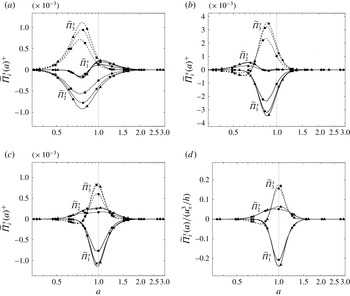
Figure 11. Cospectra of pressure–strain correlations as functions of the aspect ratio $a=\log \unicode[STIX]{x1D706}_{z}^{+}/\log \unicode[STIX]{x1D706}_{x}^{+}$ at (a) $y^{+}=1$ , (b) 15, (c) 110 and (d) $y/h=0.5$ . ——, $\widetilde{\unicode[STIX]{x1D6F1}}_{1}^{s}$ ; — ⋅ —, $\widetilde{\unicode[STIX]{x1D6F1}}_{2}^{s}$ ; — —, $\widetilde{\unicode[STIX]{x1D6F1}}_{3}^{s}$ . The symbols indicate the Reynolds number as shown in table 1.

The cospectra of the pressure–strain correlations are characterised by the aspect ratio in the wall-parallel dimensions. We here define the one-dimensional cospectra as a function of the modified aspect ratio $a\equiv \log \unicode[STIX]{x1D706}_{z}/\log \unicode[STIX]{x1D706}_{x}$ ,

(5.3) $$\begin{eqnarray}\displaystyle \widetilde{\unicode[STIX]{x1D6F1}}_{i}^{s}(a,y)=\mathop{\sum }_{\unicode[STIX]{x1D706}_{x}^{a}=\unicode[STIX]{x1D706}_{z}}\widetilde{\unicode[STIX]{x1D6F1}}_{i}^{s}(\boldsymbol{k},y). & & \displaystyle\end{eqnarray}$$

The structure of the redistribution near the wall is distinguished because the energy is transferred from $v$ to $w$ , as seen in the one-point budget in figure 9(a). The balance as a function of $a$ is given by figure 11(a). Energy transfer from $v$ to $w$ is involved in the flow structures elongated in $x$ , satisfying $\unicode[STIX]{x1D706}_{z}=\unicode[STIX]{x1D706}_{x}^{0.7}$ or $\unicode[STIX]{x1D706}_{x}^{0.8}$ . The cospectra drastically evolve within a short range in $y$ . At $y^{+}=15$ , energy is provided from $u$ mainly to $w$ for $a\approx 0.9$ that is almost isotropic. The wall-normal component $v$ receives a little energy from $w$ through elongated structures, approximately $\unicode[STIX]{x1D706}_{z}=\unicode[STIX]{x1D706}_{x}^{0.6}$ or $\unicode[STIX]{x1D706}_{x}^{0.7}$ . The two cases for higher Reynolds numbers agree well. As mentioned earlier, the cospectra in the buffer layer are universal. Above the overlap layer, the energy is redistributed from $u$ to the other components around $a=1$ . As in the case of $y^{+}=15$ , $v$ receives energy from $w$ as well through elongated structures. The total energy provided to $v$ and $w$ is approximately the same, but the aspect ratio of the fluctuations gained for $v$ is wider than that for $w$ . In addition, at this height, the two higher cases collapse fairly well. In the outer layer, the structure of redistribution is qualitatively same, but the magnitude is scaled by the outer unit $u_{\unicode[STIX]{x1D70F}}^{3}/h$ .