


1. Introduction
The first systematic investigation of the parametric excitation of a liquid layer on top of a vibrating plate was reported by Faraday (Reference Faraday1831), wherein the free fluid interface exhibits a variety of patterns. Faraday used several techniques to visualize the interfacial patterns, including the admixture of tracer particles to the fluid, investigating light reflections, as well as the correlation of light absorption in a dyed liquid to the film thickness. The dominant pattern showed a dependency on the excitation frequency as well as the amplitude, and Faraday reported the interface to oscillate with half the excitation frequency. The latter observation was challenged by Matthiessen (Reference Matthiessen1868, Reference Matthiessen1870), who observed oscillations of the surface patterns with the same frequency as the actuation (isochronous). In an attempt to clarify the contradictory results, Rayleigh (Reference Rayleigh1883) repeated the original experiments by Faraday and determined the interface to oscillate with half the driving frequency. The theoretical description of the instability of a liquid layer under harmonic oscillation was provided by Benjamin & Ursell (Reference Benjamin and Ursell1954) in the limiting case of an ideal fluid, resulting in a Mathieu equation. Depending on the forcing parameters, interface oscillations isochronous with the forcing frequency (harmonic) or with half the forcing frequency (subharmonic) are permitted, providing an explanation of the differing observations. Later on, the effects of viscosity were incorporated into the stability analysis by Kumar & Tuckerman (Reference Kumar and Tuckerman1994) utilizing Floquet analysis. While the inviscid theory results in instability even at negligible forcing, viscous effects lead to finite forcing amplitudes required to induce instability. With increasing liquid viscosity, the onset of instability shifts to higher driving amplitudes. Comparison with experiments demonstrated good agreement both for the critical forcing amplitude as well as the wavelengths observed for the instability.
Analogous to the mechanical forcing, electric fields at fluid interfaces can induce instabilities. Yih (Reference Yih1968) analysed the electrohydrodynamic equivalent to the work of Benjamin & Ursell, where an interface between a conducting and a dielectric liquid was exposed to a periodically varying electric field. The stability analysis of the inviscid fluids resulted in a Mathieu equation, but since the Maxwell stress at the interface is proportional to the square of the electric field, the interface oscillates either isochronously or with twice the frequency of the applied voltage. Around the same time, other research efforts involving electric fields acting on fluid interfaces were directed towards the response of a liquid layer to a perpendicular DC field (Taylor & McEwan Reference Taylor and McEwan1965), as well as the parametric forcing in an AC field (Briskman & Shaidurov Reference Briskman and Shaidurov1968). Further coupling mechanisms between interfacial flow and electric fields were investigated in the context of induced fluidic motion by travelling waves (Melcher Reference Melcher1966), tangential electric fields (Melcher & Schwarz Reference Melcher and Schwarz1968) and interface shaping by electric fields (Jones & Melcher Reference Jones and Melcher1973). Iino, Suzuki & Ikushima (Reference Iino, Suzuki and Ikushima1985) used an electrically induced resonance to determine the surface tension of liquid helium. More recently, Robinson et al. (Reference Robinson, Bergougnou, Cairns, Castle and Inculet2000, Reference Robinson, Bergougnou, Castle and Inculet2001, Reference Robinson, Bergougnou, Castle and Inculet2002) analysed the actuation of a liquid layer in an AC field within an ozone generator. Roberts & Kumar (Reference Roberts and Kumar2009) investigated DC and AC actuation of a thin liquid film in the context of pillaring instabilities and used the AC component as an additional means of control over the pillar dimensions. The instability of a dielectric–dielectric interface was investigated by Gambhire & Thaokar (Reference Gambhire and Thaokar2010), and conductivity effects were specifically addressed by Gambhire & Thaokar (Reference Gambhire and Thaokar2012). Also, the instability of the interface between a dielectric and a conducting liquid under AC fields accounting for Debye layer effects was studied by Gambhire & Thaokar (Reference Gambhire and Thaokar2014). Pillai & Narayanan (Reference Pillai and Narayanan2018) simulated the nonlinear evolution of the interface between an conductor and dielectric in the long-wavelength limit under an oscillatory electric field, demonstrating that the amplitudes of the Faraday waves saturate, without further growth.
Only recently, the theory of Yih (Reference Yih1968) was extended to incorporate viscous effects, similarly to the extension of Kumar & Tuckerman (Reference Kumar and Tuckerman1994) in the case of the mechanically actuated Faraday instability. First, Bandopadhyay & Hardt (Reference Bandopadhyay and Hardt2017) used Floquet theory to study the stability of a perfect dielectric on top of a perfectly conducting fluid, relating the critical voltage and the instability wavenumber. The marginal stability curve was obtained for single-frequency and multiple-frequency forcing. For single-frequency harmonic oscillations, the interface oscillates isochronously with the forcing frequency, and upon multi-frequency excitation or additional DC offset, the marginal stability curve shows both harmonic and subharmonic tongues. Ward, Matsumoto & Narayanan (Reference Ward, Matsumoto and Narayanan2019) extended the model by relaxing the assumption of perfectly dielectric and perfectly conducting liquids and based their analysis on the leaky-dielectric model. Additionally, the voltage corresponding to onset of instability for varying driving frequencies was validated for two experimental test cases, showing good agreement with theory. Due to the restrictions of the experimental set-up, no information could be retrieved about the dominant pattern wavelengths. Instead, it was reported that the experimental domain was sufficiently dimensioned to exclude any finite-size effects and that, for all observed instability modes, a multitude of wavelengths emerged. The goal of the present paper is to extend the experimental exploration of the electrostatically driven Faraday instability by analysing the spatial structure of the instability and by determining the pattern wavelengths. Especially the fact that a multitude of wavelengths was observed by Ward et al. for all experimental conditions above the critical threshold warrants further exploration, since it contrasts observations made for mechanically actuated Faraday waves. Here, usually a dominant pattern wavelength emerges, as will be discussed below.
While the experimental work on electrically actuated Faraday waves is limited, a large body of work exists on mechanically actuated Faraday waves. Using inviscid theory, Benjamin & Ursell (Reference Benjamin and Ursell1954) showed that the surface deflection of the Faraday instability can be expanded in a complete orthogonal set of eigenfunctions, which for a circular cylinder of radius  $R$ are of the form
  $S_{l,n} = J_l ( k_{l,n} r ) \cos ( l \theta )$, where
  $J_l$ denotes the Bessel function of the first kind with positive integer values l,
  $\theta$ the azimuthal coordinate, and
  $k_{l,n}$ the
  $n$th zero of
  $J^{\prime }_l (k_{l,n} R )$. These discrete modes exhibit a specific dominant wavenumber
  $k_{l,n}$ and the authors used the (2,1) mode for comparison between theory and experiments. Similar modes were observed by Dodge, Kana & Abramson (Reference Dodge, Kana and Abramson1965) and showed good agreement with the inviscid theory. Secondary instabilities at higher driving amplitudes were observed by Gollub & Meyer (Reference Gollub and Meyer1983), with successive transitions to spatial disorder of the initially ordered system. The interactions of different modes with adjacent wavenumbers were investigated by Ciliberto & Gollub (Reference Ciliberto and Gollub1984), where periodic and chaotic fluctuations between modes, as well as their superpositions, were observed. Douady & Fauve (Reference Douady and Fauve1988) studied the Faraday instability in a square container, leading to rectangular patterns. Also, the role of the meniscus at the container wall was discussed, since the presence of a sidewall meniscus influences the pattern selection. In subsequent work (Douady Reference Douady1990), the influence of the lateral boundary condition was further explored. Here, meniscus effects were suppressed by pinning the meniscus and using a brim-full container, resulting in pure modes. Contrarily, edge waves were introduced into the domain when a meniscus with a contact angle different from
  $90^{\circ }$ was present, which coupled to the parametric excitation. The time average of chaotic patterns was studied by Gluckman et al. (Reference Gluckman, Marcq, Bridger and Gollub1993), revealing a highly ordered time-averaged system due to the long-range interactions with the boundaries of a moderately large container. While previous research attempted to reduce the meniscus effects at the domain boundary by pinning the contact line, Batson, Zoueshtiagh & Narayanan (Reference Batson, Zoueshtiagh and Narayanan2013) used a different approach, where by proper selection of fluids a wetting film at the wall was established, mimicking a moving contact line. Thereby, the stress-free boundary condition was mimicked, allowing comparison with theory, without including the effects of contact line dissipation. Recently, Shao et al. (Reference Shao, Wilson, Saylor and Bostwick2021) investigated the mode selection in a brim-full container and demonstrated the emergence of the first 50 resonant modes. If a concave meniscus was present, edge waves were introduced, leading to complex mode mixing.
The influence of the boundary depends on the magnitude of the dissipation: if the dissipation is small, only a small band of wavenumbers becomes unstable above the onset voltage, and the pattern selection depends on the allowed modes of the container. For larger dissipation, a wide band of wavenumbers becomes unstable, and the pattern is selected by nonlinearities and independent of the boundary (Edwards & Fauve Reference Edwards and Fauve1994). In the literature, a variety of patterns were reported. For example, Tufillaro, Ramshankar & Gollub (Reference Tufillaro, Ramshankar and Gollub1989) observed a rectangular pattern upon initial instability formation, which transitioned into a disordered pattern with increasing driving amplitude. Edwards & Fauve (Reference Edwards and Fauve1994) observed lines, squares, circles and spirals for the single-frequency forcing, and more complex patterns upon multiple-frequency forcing. Also, the container-size influence was analysed, demonstrating that both high viscosity and high-frequency driving increase the dissipation, rendering the system independent of the boundary. The corresponding extension of the work of Kumar & Tuckerman (Reference Kumar and Tuckerman1994) to multiple-frequency forcing was performed by Besson, Edwards & Tuckerman (Reference Besson, Edwards and Tuckerman1996), and validated experimentally. In the following, amplitude- and phase-resolved measurements of hexagonal and square structures were performed by Kityk et al. (Reference Kityk, Embs, Mekhonoshin and Wagner2005). The role of the frequency shift between the different driving frequencies was analysed by Epstein & Fineberg (Reference Epstein and Fineberg2008), resulting in a criterion for mode mixing to occur. For additional information on Faraday instabilities, the reader is referred to dedicated reviews on this topic, e.g. Nevolin (Reference Nevolin1984), Miles (Reference Miles1990), Perlin & Schultz (Reference Perlin and Schultz2000) and Müller, Friedrich & Papathanassiou (Reference Müller, Friedrich and Papathanassiou2011).
From this short overview over the literature of mechanically excited Faraday waves, it is apparent that both boundary-dominated systems as well as boundary independent systems exhibit typical pattern wavelengths, which can even be retained after secondary transitions to chaotic regimes. The present work aims to clarify which wavelengths and instability patterns are observed for the electrostatically driven Faraday instability, in order to extend the experiments performed by Ward et al. (Reference Ward, Matsumoto and Narayanan2019). Also, we wish to scrutinize the reported emergence of a multitude of wavelengths, without the presence of defined eigenmodes, as this observation differs from the results obtained for mechanical actuation. The remainder of the paper is structured as follows: in § 2, the experimental set-up and the light refraction-based method to measure the pattern wavelength are introduced, jointly with the interface reconstruction algorithm and the theoretical description. In § 3, experimentally obtained critical voltages and pattern wavelengths are presented for varying electrolyte conductivity and liquid viscosity. Furthermore, the spatial structure of the instability is presented, revealing the existence of discrete instability modes and superpositions thereof. Also, the transition to a boundary-independent spatial structure of the instability is observed for higher viscosity and driving frequency. Finally, the results are summarized and discussed in § 4.
2. Experimental details and theoretical description
2.1. Experimental set-up
The experimental set-up is shown in figure 1(a). It consists of a cylindrical chamber, a high voltage power source (HVS448 6000D, LabSmith, USA), a CMOS camera (FASTCAM Mini AX, Photron, Japan) with a macro objective (SWM VR ED IF Micro 1:1, Nikon, Japan), a LED panel (NL480, NEEWER, China) and a mirror cut from a silicon wafer. The central part of the set-up is the cylindrical chamber that is described in the following and represents a modification of the set-up used by Ward et al. (Reference Ward, Matsumoto and Narayanan2019). A circular plate made of stainless steel with a rectangular cut out of  $4.6\,{\rm cm} \times 4.6\,{\rm cm}$ serves as the bottom electrode, leading to an observation region size of approximately
  $3.5\,{\rm cm} \times 3.5\,{\rm cm}$. In order to allow leakage free optical access from below, a rectangular glass window is glued into the cut out using an UV adhesive (NOA68, Thorlabs, Germany), such that the electrode and the window form a planar connection at the inside of the chamber. A glass cylinder of height
  $h \approx h_1 + h_2$ and diameter
  $d$ allows optical observations from the side. In the present study
  $d= 125$,
  $h_1 = 5$, and
  $h \approx 35\,{\rm mm}$. The cylinder is arranged between the bottom and the top electrode by a non-conductive plastic holder, fixed by a set of plastic screws. Gaskets (EPDM, APSOparts, Germany) between the glass cylinder and the electrodes assure a leakage free connection. A filling port located close to boundary of the cylindrical top plate with a diameter of 1 cm allows filling the chamber with liquids. At the surface of the upper electrode facing the inside of the chamber, a grating is applied using laser ablation, with a line distance of 0.5 mm. The grid is imaged through the liquid–liquid interface, and due to refraction, a distorted image is recorded (see figure 1(b), red). From the distorted image, the original liquid–liquid interface can be reconstructed, following the procedure outlined by Moisy, Rabaud & Salsac (Reference Moisy, Rabaud and Salsac2009), as detailed in § 2.5.

Figure 1. Experimental set-up and image processing principle. (a) Schematic of the experimental set-up used throughout this study. A high voltage source is connected to the upper and lower electrodes of a cylindrical container with diameter  $d$. The container is filled with KCl solution up to a certain height
  $h_2$. With a layer of silicone oil of height
  $h_1$ above the KCl solution the container is entirely filled. On the upper electrode surface, a grid is formed by laser engraving. The grid is imaged during an experiment by a high-speed camera via a mirror. Illumination is performed using a LED panel with a diffusor from below. (b) Schematic of the measurement principle. The grid with a line spacing of 0.5 mm at the upper electrode is imaged and appears distorted due to refraction at the liquid–liquid interface. From the distorted image, the original interface shape can be reconstructed.
To allow optical inspection of the chamber, a rectangular mirror fabricated from a silicon wafer is mounted onto a goniometer (OWIS, Germany). It redirects the optical path by  $90^{\circ }$, allowing recording by the horizontally oriented high-speed camera via a macro objective. The goniometer allows fine adjustment of the optical path in two directions. The illumination of the chamber is performed by a LED panel with a diffusor through the glass window from below, leading to a dark grid appearing on a bright background. An electric potential difference can be applied between the top and the bottom electrode via connecting each to a separate channel of a high voltage source. The latter allows generating an AC voltage signal of
  ${\pm }6000\,{\rm V}$ peak to peak, within a sufficiently large frequency range. At each of the electrodes, a voltage of the form
  $U_0/2 \sin ( 2 {\rm \pi}f )$ with different sign is applied, so that an overall potential difference
  $U_0\sin ( 2 {\rm \pi}f )$ is present. The camera and the high voltage source are both connected to a computer and can be controlled via the appropriate software from the hardware supplier (Photron Fastcam Viewer and Labsmith Sequence).
2.2. Experimental procedure
In order to minimize the influence of any pollutant on the liquid and interfacial properties, all parts of the chamber are cleaned thoroughly by rinsing them with isopropanol, followed by deionized (DI) water. Then, the parts are blown dry in a nitrogen stream and subsequently assembled to form a leakage free chamber, as sketched in figure 1(a). The chamber is then placed onto a support rack on an air-cushioned optical table, and aligned horizontally. Prior to the experiments, the optical components are aligned to ensure a distortion-free, focused image of the grid at the upper electrode. Afterwards, the chamber is filled by first pipetting the bottom liquid through the filling hole up to a level  $h_{2}$ and then carefully adding a layer of silicone oil above the bottom liquid by the same technique, until it overflows the filling hole. The liquids used in this study and their properties are described in § 2.3. Before filling, the liquids are degassed within an excesscator for at least 30 min to avoid gas bubbles in the set-up. The filling port is being covered to avoid dust or other pollutants to enter the chamber after filling. Subsequently, the electrodes are connected to the two separate channels of the high voltage source. Then, the grid is focused by adjusting the focal plane of the objective.
In order to measure the critical voltage for a given pair of liquids and a given excitation frequency, the driving signal is chosen with an amplitude well below the theoretically calculated critical voltage. Then, the excitation is switched on and the system response, i.e. the interface oscillation, is observed for three minutes, both through the camera image and through the side wall of the glass cylinder. The excitation voltage amplitude is subsequently increased, and the experiment is repeated as described above. In most cases, it is possible to clearly distinguish between edge waves stemming from the domain boundary and a critical interface response, i.e. Faraday waves. If the response of the system exhibits Faraday waves, the image of the grid is recorded for 1 s at a framerate of 1000 f.p.s. (f.p.s. – frames per second), starting 150 s after the voltage has been applied. Responses without dedicated Faraday patterns are not recorded to reduce data overhead. In case of an unclear or mixed system response, recordings are made for subsequent clarification via image evaluation. As described in § 2.5, the data are post-processed in order to identify the type of system response. In case of strong instabilities, it is necessary to stop an experiment before three minutes have passed in order to prevent the bottom phase to touch the upper electrode, since the deformation amplitude of the interface may increase continuously until the interface contacts the upper electrode locally. In case of electric breakdown, liquid of the bottom phase adheres to the upper electrode and influences the electric field in subsequent experiments, thus necessitating a disassembly and cleaning of the chamber. In case of the interface touching the upper electrode, the data were excluded from the wavelength evaluation, while they were included in the evaluation of the critical voltage.
2.3. Fluids
The conducting lower phase consists of mixtures of DI water (specific resistance 18.2 M $\Omega$ cm, Milli-Q Integral 3, Millipore) and glycerol (CAS: 56-81-5, Quality:
  $\geq$99.5 % water free, Sigma-Aldrich and Carl Roth, both Germany). Three different mass fractions of glycerol are used: 0 wt%, 60 wt% and 70 wt%. Before use, the two components were thoroughly mixed by magnetic stirrer for at least 24 h to ensure a homogeneous mixture. A defined amount of potassium chloride (KCl, CAS: 7447-40-7, Quality: ACS Reagent, Sigma-Aldrich, Germany) is added to the bottom phase to increase the conductivity. A concentration of
  $c_{KCl} = 0.001\,{\rm mol}\,{\rm l}^{-1}$ is used, except for the experiments performed to specifically measure the influence of the concentration. The fluid data reported in table 1 and the interfacial tensions in table 2 were determined with this particular concentration. For the sake of simplicity, the bottom phase fluids are identified by their glycerol mass fraction as 0 wt%, 60 wt% and 70 wt%. Three silicone oils of different viscosity are used (Silikonöl AK 0.65, Silikonöl B1 and Silikonöl B5, Silikon Profis, Germany) as dielectric liquids, and hereinafter identified according to their kinematic viscosity as 0.65, 1 and 5 cSt. The fluid properties are summarized in table 1 and the interfacial tensions in table 2. In Appendix A we report how the fluid properties were measured.
Table 1. Physical properties of the used liquids. The upper row shows data for the dielectric liquids representing the upper phase, while the bottom row depicts data for the conducting liquids of the lower phase. Mean values together with standard deviations are reported. In case of viscosity and dielectric permittivity, the values are calculated (c), or taken from the respective data sheet (l).

Table 2. Interfacial tensions between specific fluids. Mean values together with standard deviations are reported.

2.4. Theoretical description
The theoretical description of the instability is a modification of the approach by Bandopadhyay & Hardt (Reference Bandopadhyay and Hardt2017), where the upper liquid is considered to be a perfect dielectric, and the lower liquid to be a perfect conductor. Different from Bandopadhyay & Hardt (Reference Bandopadhyay and Hardt2017), it is assumed that the upper layer thickness is small compared with that of the lower layer,  $h_1/h_2 \ll 1$, in order to simplify the resulting system of equations. The theoretical approach is described in Appendix B, and only the key ideas will be summarized in the following. Apart from the work by Bandopadhyay & Hardt (Reference Bandopadhyay and Hardt2017), a theoretical description exists that takes into account that the dielectric phase can have a non-negligible conductivity (Ward et al. Reference Ward, Matsumoto and Narayanan2019). The authors have shown that the results by Bandopadhyay & Hardt (Reference Bandopadhyay and Hardt2017) are reproduced in the limiting case of an infinite conductivity ratio. This assumption is specifically revisited in § 3.1.
The system under investigation in Bandopadhyay & Hardt (Reference Bandopadhyay and Hardt2017) consists of two immiscible fluid layers with thicknesses  $h_{1}$,
  $h_{2}$ between two planar electrodes, as depicted in figure 1(a), extending infinitely in the lateral direction. The density
  $\rho _i$ and the dynamic viscosity
  $\eta _i$ of both fluids are given, as well as the relative permittivity of the dielectric liquid
  $\epsilon _1$. The interface is located at the
  $z$-position
  $ \zeta (\boldsymbol {x}_s,t)$, where
  $\boldsymbol {x}_s$ denotes the position in the
  $xy$-plane. The governing equations of the problem are Laplace's equation of electrostatics in the dielectric liquid, and the continuity and Navier–Stokes equations in both liquids. The problem is solved using a domain perturbation method for the fluid interface in combination with Floquet theory. Following the mathematical derivation outlined in Appendix B, a generalized eigenvalue problem of the form
 \begin{equation} \boldsymbol{\mathsf{A}}\boldsymbol{Z} = Ma\,\boldsymbol{\mathsf{B}}\,\boldsymbol{Z}, \end{equation}
is obtained, with the matrices  $\boldsymbol{\mathsf{A}}$,
  $\boldsymbol{\mathsf{B}}$ and the vector
  $\boldsymbol {Z}$ containing the Fourier coefficients of
  $\zeta$. The parameter
  $Ma$ denotes the Mason number, which is defined as
 \begin{equation} Ma = \frac{\epsilon_1 U_0^{2}}{4 \eta_1 \omega h_1^{2}}, \end{equation}
where  $\omega$ denotes the angular frequency of the driving electric field. It is important to note that the theoretical description is non-dimensional, however, in the following, the results are shown in dimensionalized form in order to make them more accessible to the reader. As the problem converges for a finite number of Fourier modes, as shown by Bandopadhyay & Hardt (Reference Bandopadhyay and Hardt2017), (2.1) can be used to obtain the marginal stability curve for a given set of fluid pairs, driving frequency and perturbation wavenumber
  $k$. As shown in the example displayed in figure 2(a), the marginal stability curve takes the shape of tongues in the voltage–wavenumber space, characteristic for Faraday instabilities. The lowest voltage for a given fluid pair and driving frequency corresponds to the critical voltage
  $U_{crit}$ above which the Faraday instability is expected to occur. The corresponding wavenumber
  $k_{th}$ is the most unstable wavenumber, which we expect to observe close to the critical voltage.

Figure 2. Theoretical results obtained for the fluid pair of 0.65 cSt silicone oil and 0 wt% glycerol (described in § 2.3). (a) Marginal stability curve for a driving frequency of  $f=2$ Hz. Different wavenumbers become unstable at different voltages, and the critical voltage
  $U_{crit}$ represents the voltage corresponding to onset of instability considering all wavenumbers. (b) Stability map. For otherwise fixed parameters, the critical voltage is plotted vs the driving frequency, and represents the experimentally measurable stability curve. (c) Critical wavelength as a function of critical voltage. Corresponding wavelengths are expected to be observed close to the onset of instability.
Experimentally, the marginal stability curve for a given driving frequency is not readily measurable. Upon increasing the driving voltage amplitude at a given frequency, a specific wavenumber  $k_{th}$ becomes unstable first, at a corresponding critical voltage amplitude
  $U_{crit}$. With increasing amplitude, more wavenumbers become unstable. However, in the absence of an exclusion mechanism, e.g. a finite domain size, we can only determine the onset of instability, not the onset for each individual wavenumber
  $k$. However, the critical voltage
  $U_{crit}$ and the corresponding wavelength
  $\lambda _{th}$ can be measured for different driving frequencies, as shown in figure 2(b,c). For the comparison with experimental observations, both the critical voltage
  $U_{crit}$ and the corresponding wavelength
  $\lambda _{th}$ are used in the following. Therefore, we will compute both quantities for varying driving frequencies, with the experimental parameters as input values, and use them to assess the accuracy of the theoretical model.
Before proceeding to the evaluation of the experiments, it is important to emphasize that the utilized stability analysis is linear. Therefore, it is not possible to distinguish the nature of transition from the rest state to an oscillatory state of the interface. Above a critical voltage, the system changes its qualitative long-time asymptotic behaviour, as the rest state becomes unstable. Then, at least one stable oscillatory state emerges, which is referred to as bifurcation. In this regime, an infinitesimal perturbation grows exponentially, until nonlinearities limit the growth. Bifurcations can be further characterized depending on the transitions between stable solution branches (Cross & Hohenberg Reference Cross and Hohenberg1993): in case the transition from the stable rest state to the oscillatory state is continuous as a function of the control parameter (here: forcing voltage amplitude), it is supercritical. Upon reduction of the forcing below the critical voltage, the system returns to its rest state. On the other hand, it is also possible that an oscillation persists if the forcing is reduced below the onset voltage. Then, both the rest state as well as at least one oscillatory state are stable simultaneously, which is denoted as subcritical bifurcation. Here, the nonlinearities promote the instability instead of damping it. Subcritical bifurcation manifests itself as hysteresis and an ambiguity in the determination of the instability threshold, where the instability requires a certain amount of forcing to develop from the rest state, and a second threshold emerges, below which the rest state is recovered. For mechanical forcing of Faraday instabilities, the existence of hysteresis has been discussed and observed (Douady Reference Douady1990; Craik & Armitage Reference Craik and Armitage1995; Chen & Wu Reference Chen and Wu2000), and recently, the influence of the forcing and dissipation on the dispersion relation has been revisited analytically (Rajchenbach & Clamond Reference Rajchenbach and Clamond2015). In that context, it was shown that the detuning of the oscillation frequencies of Faraday waves compared with the eigenfrequencies of the unforced, undamped interface modes plays a crucial role, as well as the viscous dissipation. As was shown by Rajchenbach & Clamond, the nature of the bifurcation depends on the exact parameters of the dispersion relation, and can differ between short and long wavelengths compared with the liquid layer thickness, leading to supercritical bifurcation or subcritical bifurcation, respectively.
In the aforementioned works, a single liquid layer in contact with air was forced mechanically, but subcritical bifurcation can also be observed for electrostatic actuation. In agreement with the work by Rajchenbach & Clamond (Reference Rajchenbach and Clamond2015), Pillai & Narayanan (Reference Pillai and Narayanan2018) showed numerically that an electrostatically forced thin film exhibits subcritical bifurcation, with hysteresis occurring. For driving amplitudes below the onset voltage according to linear stability theory, an initial perturbation can either develop into Faraday waves, or decay to the rest state. In addition to the hysteresis, it was shown that the Faraday instability can also exhibit nonlinearly saturated waves. Upon further increase of the driving amplitude, the instability continues to grow slowly, until the interface spikes abruptly, locally contacting the electrode.
Studying the full nonlinear problem for our system is beyond the scope of this work, however, these previous results based on the long-wave approximation have two implications for the interpretation of our experiments. First, it is possible that Faraday waves are present below the threshold predicted by linear stability analysis, if significant initial perturbations are present, e.g. introduced by edge waves. Then, nonlinearities can promote the oscillations. Thus, the onset voltage resulting from linear stability theory represents an upper limit for the onset of instability. Second, the interface deformation amplitudes can be limited to finite values by nonlinearities, in contrast to the indefinite growth expected from the linear theory. Also, upon increase of the driving amplitude, the interface is expected to show abrupt spiking, transitioning from an oscillating state with a slowly changing amplitude to a mode with rapidly growing local deformations.
2.5. Data evaluation
For the processing of the experimental data, a refraction-based evaluation routine was used to determine the dominant wavelength of the instability pattern. In figure 3(a), a schematic of the measurement principle is shown. The reference grid at the upper electrode (depicted in black) is imaged through the liquid–liquid interface. Due to the difference of the refractive indices, the image of the grid (depicted in red) is distorted. Light rays passing through horizontal sections of the interface are not altered, whereas rays crossing the interface at positions with a non-zero gradient  $\boldsymbol {\nabla } h$ are refracted according to Snell's law (
 $\sin \theta _1 n_1 = \sin \theta _2 n_2$). The difference between the original grid and the recorded grid is referred to as the displacement field
  $\Delta \boldsymbol {x}$. In the following, we utilize the measurement principle outlined by Moisy et al. (Reference Moisy, Rabaud and Salsac2009), who derived the relation between the displacement field
  $\Delta \boldsymbol {x}$ and the surface gradient
  $\boldsymbol {\nabla } h$ introducing the following assumptions: first, paraxial optics is assumed, which requires a small observation field compared with the distance between the objective and the observed grid (here: 3.5 cm vs 35 cm). Also, they assumed a small slope of the interface, such that the angle between the surface normal
  $\boldsymbol {n}$ and the unit vector in
  $z$-direction is small, and that the deformation amplitude is small (
 $(h_1-h)/h_1 \approx 0$), where
  $h_1$ is the layer thickness corresponding to the undistorted interface. Then, the relation between the surface gradient
  $\boldsymbol {\nabla } h$ and the displacement field
  $\Delta \boldsymbol {x}$ is linear, given as
 \begin{equation} \boldsymbol{\nabla} h ={-}\frac{a_{cal}}{h^{*}} \Delta \boldsymbol{x}, \end{equation}
where  $a_{cal}$ is a calibration factor in units of mm px
 $^{-1}$ obtained from a reference image of a flat interface, and
  $h^{*}$ is an effective height obtained from the optical configuration as
 \begin{equation} h^{*} = \left(\frac{1}{\alpha h_1}-\frac{1}{H_{cam} + h_1} \right)^{{-}1}. \end{equation}
Here,  $\alpha = 1-n_2/n_1$ denotes the difference of the refractive indices and
  $H_{cam}$ the distance between the objective and the interface. In our situation, the second term of (2.4) is negligible due to the large ratio
  $H_{cam}/h_1\ll 1$.

Figure 3. Post-processing steps of the image data. (a) Schematic of the refraction-based image evaluation. A reference grid at the top electrode (black) is imaged through the liquid–liquid interface. Due to different refractive indices of the liquids, the recorded image is distorted (red). (b) Example of a displacement pattern. The displacement field  $\Delta \boldsymbol {x}$ can be used to determine the surface gradient
  $\boldsymbol {\nabla } h$, which in turn can be used to reconstruct the interface deflection
  $\Delta h = h-h_1$. (c) Fourier power spectrum corresponding to (b). The power density is plotted as a function of the wavenumber magnitude
  $k$ and exhibits several peaks: Peaks (I) and (III) result from the numerical reconstruction algorithm (see text for details). The peak corresponding to the dominant pattern wavelength
  $\lambda$ (II) is found in an intermediate wavenumber range. Here,
  $\lambda = 3M a_{cal} /k = 6.85\,{\rm mm}$.
Equation (2.3) demonstrates that the displacement field for a constant surface gradient  $\boldsymbol {\nabla } h$ will increase with increasing layer thickness
  $h_1$ and a larger difference between the refractive indices
  $n_1$,
  $n_2$. While the surface gradients are used to reconstruct the interface
  $h(x,y)$, it is important to note that we will not rely on the absolute values of the reconstructed interface deformation, but rather on the pattern wavelengths. While the absolute values of
  $h$ are sensitive to variations in
  $\boldsymbol {\nabla } h$ as well as
  $h^{*}$, the obtained pattern wavelengths are not. The evaluation scheme includes three distinctive steps: first, the surface gradients
  $\boldsymbol {\nabla } h(x,y)$ are generated from the displacement field recorded during the experiments. Second, the interface shape
  $h(x,y)$ is reconstructed, with one exemplary resulting data set shown in figure 3(b). In a third step, the dominant pattern wavelength is extracted using a Fourier transform and the corresponding power spectrum, as shown in figure 3(c). The details of the evaluation are described in Appendix C.
3. Results and discussions
In this section, we present the experimental results for the electrically induced Faraday instability. We focus on the critical voltage and report the dominant pattern wavelengths. Typically, for one fixed set of experimental parameters, the system shows different characteristic responses with increasing voltage amplitudes. The electric actuation leads to two competing effects: at the sidewall (i.e. the boundary of the container), the meniscus of the dielectric–electrolyte interface oscillates due to the applied Maxwell stress. As the applied Maxwell stress depends quadratically on the electric field strength at the interface, a harmonic driving with a frequency  $\omega$ leads to an actuation of the meniscus with a frequency of
  $2 \omega$. Further, the Faraday instability occurs above a critical voltage, which leads to oscillations with a frequency of
  $\omega$ when forced with a single frequency. At low excitation amplitudes, the actuation of the meniscus leads to small interface deformation with twice the excitation frequency, which is barely noticeable initially. With increasing amplitude, the actuation of the meniscus becomes more prominent and waves penetrate from the boundary of the container into the domain. A circular pattern is created, with the waves moving into the centre of the domain. This effect is similar to the edge-wave actuation in the case of mechanically excited Faraday waves. With further increasing excitation amplitude, Faraday waves start to appear, initially only with a small amplitude. Both edge waves as well as Faraday waves are present simultaneously. A further increase of the amplitude leads to the formation of stronger Faraday waves, which begin to dominate the system. Then, a distinct range of driving amplitudes exists, where the pattern becomes stable for long times after an initial growth phase. A similar phenomenon was observed by Pillai & Narayanan (Reference Pillai and Narayanan2018) and attributed to nonlinear effects. When some specific excitation amplitude is exceeded, however, the Faraday waves continue to grow until they make abrupt, local contact with the upper electrode and lead to an electric connection between both electrodes. Then, the power supply shuts off automatically. In the following, all parameter combinations that lead to Faraday waves are denoted as critical, since the voltage exceeded the critical voltage. All other parameter combinations with edge waves only are denoted as subcritical, since no Faraday patterns emerge during the experiment. We want to emphasize that here the terms ‘critical’/‘subcritical’ refer to the existence of instabilities, not to the nature of bifurcation as discussed in § 2.4.
3.1. Effect of the salt concentration
As we have discussed in § 2.4, the theoretical model used to predict the instability threshold is based on the perfect-dielectric/perfect-conductor assumption. As was shown by Ward et al. (Reference Ward, Matsumoto and Narayanan2019), the description using the leaky-dielectric model reduces to the perfect-dielectric/perfect-conductor model if the conductivity ratio between the liquids is sufficiently high. In order to assess the validity of the perfect-conductor assumption, we have varied the KCl concentration in the lower liquid (DI water) from  $1\times 10^{-4}$ to
  $1\times 10^{-1}\,{\rm mol}\,{\rm l}^{-1}$ at otherwise fixed parameters (silicone oil viscosity 0.65 cSt, driving frequency 10 Hz).
In figure 4(a), the experimentally obtained stability map is shown. As is visible, the critical voltage is not strongly affected by the salt concentration. It is slightly increased at  $c_{KCl}=1\times 10^{-4}\,{\rm mol}\,{\rm l}^{-1}$ and slightly reduced at
  $c_{KCl}=1\times 10^{-3}\,{\rm mol}\,{\rm l}^{-1}$. Since no clearly distinguishable trend is present, we attribute the differences to experimental uncertainties. One potential source of uncertainty are the edge waves penetrating into the central region of the system, superposing and obscuring the Faraday waves. Also, since the detection relies on surface gradients, the accuracy at small surface gradients is limited. Nevertheless, the experimentally obtained critical voltages show fair agreement with the theoretically predicted value of
  $V_{crit}=2393$ V (indicated as a dashed line).

Figure 4. Influence of the lower-phase salt concentration on the instability for a forcing frequency of 10 Hz. (a) Experimentally obtained stability map together with the theoretical prediction for the critical voltage obtained from the perfect-dielectric/perfect-conductor model (critical voltage  $V_{crit}=2393$ V). (b) Experimentally determined pattern wavelength together with the theoretical prediction for the dominant wavelength obtained from the perfect-dielectric/perfect-conductor model (
 $\lambda =11.35$ mm). Each data point corresponds to one critical voltage in (a). The error bars represent the standard deviation of the obtained wavelength determined within one experiment.
In figure 4(b), the experimentally determined pattern wavelengths corresponding to the critical voltages of figure 4(a) are shown. As is visible, the change of wavelengths between different driving amplitudes is of the same order of magnitude as the differences over the salt concentration. The experimentally obtained values show good agreement with the theoretically predicted value of  $\lambda =11.35$ mm. Since the experimental results scatter around the theoretically predicted value, the experiments indicate that the salt concentration does not significantly influence the resulting wavelength in the range of concentrations studied. Therefore, the conductivity difference between both liquids is sufficiently large to allow us to describe the instability using the perfect-dielectric/perfect-conductor model. For the experiments described in the following, we proceed with a constant salt concentration of
  $c_{KCl}=1\times 10^{-3}$ mol l
 $^{-1}$.
3.2. Effect of the viscosity of the dielectric fluid
In this section, we study the influence of the viscosity of the dielectric fluid by analysing data from experiments with different silicone oils. While we wish to specifically vary the viscosity, changing the dielectric fluid leads to variations in other parameters as well. A summary of the liquid properties can be found in § 2.3. For each driving frequency and voltage amplitude, one experiment was performed. The pattern wavelengths are obtained following the procedure outlined in § 2.5 and Appendix C. For some experiments, no dominant pattern wavelength could be reported, while the corresponding condition is noted as critical in the stability map, i.e. when the interface touched the upper electrode.
In figure 5, the experimentally obtained stability maps and the resulting pattern wavelengths are displayed, with the theoretical predictions of the linear stability theory shown as black lines. For the kinematic viscosity of 0.65 cSt, the critical voltage shows partial agreement with the theory. For low excitation frequencies, the onset of the Faraday instability occurs at a significantly higher driving amplitude than predicted. Subsequently, with increasing excitation frequency, the difference between theory and experiments becomes smaller, and at high frequencies, the critical voltage is over-predicted by theory. The pattern wavelength shows good agreement with theory, and for the multiple critical driving amplitudes at a fixed frequency, similar wavelengths are obtained.

Figure 5. Influence of the viscosity of the dielectric fluid on the instability and the pattern wavelength. DI water with added KCl of  $c=1\times 10^{-3}$ mol l
 $^{-1}$ forms the lower phase. (a–c) Experimentally obtained stability maps for different viscosities. (d–f) Dominant wavelengths of the wave patterns for different viscosities. Each data point corresponds to one critical voltage in (a–c). The error bars represent the standard deviation of the obtained wavelength determined within one experiment. In all cases, the theoretical predictions are displayed as black lines.
In figure 5(b,e), results for the silicone oil with a viscosity of 1 cSt are shown. Here, the theory over-predicts the onset of instability compared with the experiments, while a qualitative agreement is apparent. The difference could be explained by an uncertainty of the upper layer thickness. The Maxwell stress at the interface strongly depends on the layer thickness, and a decrease of the thickness of 0.25 mm already increases the Maxwell stress by 10.8 %. This means that to fix the Maxwell stress with decent accuracy, the layer thickness needs to be determined with very high accuracy. The pattern wavelength, on the other hand, shows good agreement between theory and experiments, especially for large excitation frequencies. Below 5 Hz, the experimentally obtained wavelengths are smaller than predicted. However, since in that case the wavelengths are of the same scale as the region of interest, the measurement becomes less accurate. Overall, we conclude that there is a quantitative agreement between the experimental and the theoretical data for the pattern wavelength.
For the oil viscosity of 5 cSt, we report experimental results only up to 6 Hz, as can be seen in figure 5(c, f). At higher excitation frequencies, the lower liquid contacted the upper electrode without the occurrence of Faraday waves. Instead, local Taylor cones formed and protruded to the electrode. For the experimental data we were able to obtain, the agreement of the critical voltage and pattern wavelength is apparent between theory and experiments, with some discrepancies at low frequencies. Again, in that case the pattern wavelength is of the same scale as the observation region, and thus the wavelength might be underpredicted.
Overall, the experimentally obtained pattern wavelengths and the theoretical predictions agree well. The oil viscosity only has a small influence on the wavelength and the critical voltage. This trend conforms with the theoretical predictions made by Bandopadhyay & Hardt (Reference Bandopadhyay and Hardt2017). Also, for a given frequency, a change of driving amplitude above the onset of the Faraday instability has only little effect on the resulting pattern wavelength, since the resulting wavelengths are reproduced for different driving voltages.
3.3. Effect of the viscosity of the electrolyte
In this section, we discuss the influence of the lower layer's viscosity on the stability of the system and the wave patterns. For this purpose, glycerol–water mixtures with different glycerol mass fractions, expressed as weight per cent (wt%), were used. For the electrolyte with 60 wt% glycerol, the dynamic viscosity is 9.38 mPa s and for 70 wt% glycerol it is 19.69 mPa s. The upper layer was silicone oil with a kinematic viscosity of 0.65 cSt. Again, for each excitation frequency and voltage amplitude, one experiment was performed.
In figure 6, the experimentally obtained stability maps and pattern wavelengths are shown, where the data for 0 wt% glycerol correspond to figure 5(a,d). The data for 60 wt% glycerol show a good agreement between the experimentally measured and the theoretically predicted critical voltage. Compared with the experiments with 0 wt%, the range of Faraday patterns that do not grow indefinitely is smaller. Also, compared with the previous experiments, the critical voltage is higher, and its slope increases with the viscosity of the lower phase. The pattern wavelength is represented well by the theoretical model over the whole range of excitation frequencies, as can be seen from figure 6(e).

Figure 6. Influence of the viscosity of the dielectric fluid on the instability and the pattern wavelength. Silicone oil with 0.65 cSt forms the upper phase, and the KCl concentration in the lower phase is  $c=1\times 10^{-3}$ mol l
 $^{-1}$. (a–c) Experimentally obtained stability maps for different electrolytes. (d–f) Dominant wavelengths of the wave patterns for different electrolytes. Each data point corresponds to one critical voltage in (a–c). The error bars represent the standard deviation of the obtained wavelength determined within one experiment. In all cases, the theoretical predictions are displayed as black lines.
Increasing the glycerol mass ratio to 70 wt% leads to even higher critical voltages, as can be seen from figure 6(c). Here, the agreement between the stability map and the theoretically predicted critical voltage is good as well, with increasing deviations at higher excitation frequencies. As is visible, the range of Faraday patterns that do not exhibit indefinitely growing amplitudes is even smaller than for 60 wt%. Often, only one driving voltage exhibited a Faraday pattern that was stable for longer times, and an increase of the driving amplitude lead to a continuously growing interface deflection and ultimately an electric connection between both electrodes. Again, the experimental and the theoretical data for the pattern wavelengths show good agreement.
3.4. Spatial structure of the wave patterns
So far, we have focused on the wavelength of the emerging patterns, without further detailing their spatial structure. The theoretical considerations presented in § 2.4 assume an infinite domain without lateral boundaries. While the dominant wavelength and critical voltage are predicted, no spatial structure of the waves can be derived from the presented linear stability theory. Here, nonlinear theory would be required (Chen & Viñals Reference Chen and Viñals1999), which is beyond the scope of this work. Nevertheless, we can use experiments to characterize the resulting spatial structure. In the previous work by Ward et al. (Reference Ward, Matsumoto and Narayanan2019), the experimental results were obtained using a fluid domain of similar size and with similar fluid pairs, but due to imaging in side view, the authors could not distinguish specific modes or determine the wavelengths. They concluded that the domain size was sufficient such that the instability patterns were not influenced by the lateral boundaries, and reported that a multitude of wavelengths are observed during all unstable configurations. In the following, we report the spatial structure of the observed wave patterns and compare them with the observations made for mechanically excited Faraday waves.
Before continuing with our experimental results, it is instructive to draw from the analogy to mechanically induced Faraday waves. As was shown by Benjamin & Ursell (Reference Benjamin and Ursell1954), the surface deflection of Faraday waves can be expressed as a series of a complete orthogonal set of eigenfunctions, assuming ideal fluids, taking the form
 \begin{equation} \Delta h = \sum a_{l,n}(t) J_l\left( k_{l,n} r \right) \cos \left( l \theta \right), \end{equation}
where  $a_{l,n}(t)$ denotes a time-dependent amplitude,
  $J_l$ the Bessel function with the azimuthal node number
  $l$ and
  $k_{l,n}$ the
  $n$th root of
  $J_l^{\prime } ( k_{l,n} R )$. In a recent work by Shao et al. (Reference Shao, Wilson, Saylor and Bostwick2021), the modes of the mechanical Faraday instability in a circular container of finite size were characterized, demonstrating similar mode forms. By changing the frequency and the amplitude of the excitation, they were able to observe a large range of pure modes. In figure 7, some exemplary theoretical modes following the form of (3.1) are depicted. Apparently,
  $l$ leads to an increase of the number of nodes in the circumferential direction, and
  $n$ leads to more nodes in the radial direction. As prominently visible in figure 7(b,c), a nearly unperturbed region is found at the centre of the domain, enclosed by a circular region of larger deflections. Also, as was discussed for example by Ciliberto & Gollub (Reference Ciliberto and Gollub1984), mode mixing can occur between modes with similar
  $k_{l,n}$, which can lead to excitation of modes of odd parity with respect to a specific axis, as shown in figure 7(d). Owning to the substantial differences between the corresponding systems studied in the literature and our system (air vs liquid as the upper layer; mechanical vs electrical actuation), it is not clear a priori if the system studied by us will exhibit a dominant boundary influence or if it will behave as an unbounded domain. In addition, Shao et al. (Reference Shao, Wilson, Saylor and Bostwick2021) illuminated the role of the boundary meniscus, leading to waves travelling into the domain, which in the case of mechanical actuation stem from a contact angle different from
  $90^{\circ }$ at the container side wall. The superposition of Faraday waves and edge waves leads to complex instability patterns deviating from the modes of (3.1).

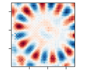
Figure 7. Theoretically predicted Bessel modes of the form  $\Delta h = J_l( k_{l,n} r ) \cos ( l \theta )$, where
  $l$ is the azimuthal mode number and
  $k_{l,n}$ are the roots of
  $J_l^{\prime }( k_{l,n} R )$. (a–c) Exemplary modes with different mode numbers
  $l, n$ are shown. The circular region corresponds to the circular interface of the experiments. Red values corresponds to the peaks of the interface deflection
  $\Delta h$, and blue to the valleys. Due to the limited field of view, only the central region is observed in our experiments, indicated as black squares. (d) A superposition of two modes creates patterns with odd parity.
In the following, the instability patterns at the moment of largest deflection during an oscillation period are shown. Thus, they depict an instantaneous surface profile and contain no information about the time evolution or the pattern dynamics. As was revealed by Gluckman et al. (Reference Gluckman, Marcq, Bridger and Gollub1993) in the context of mechanically actuated Faraday patterns, systems that appear disordered instantaneously can exhibit an ordered time average over long times. The interface deflection  $\Delta h$ is shown normalized, with the highest and lowest values shown in colour (red and blue), such that the spatial structure is visible. Each image is normalized by assigning red to the maximum and blue to the minimum value present within the image, in order to emphasize the spatial structure. As we have outlined in § 2.2, the instability is recorded 150 s after the voltage is switched on, such that the patterns are able to reach a quasi-steady state. For the sake of brevity, not every experimentally obtained interface deformation is shown, but rather representative modes for specific frequencies and amplitudes. Only three combinations of oils and electrolytes are shown, since the other experimental configurations show similar behaviour without qualitatively new information.
In figure 8, Faraday patterns for the silicone oil with 0.65 cSt in combination with water are shown, where the excitation frequency and the theoretically predicted wavelength are displayed at the top of each column. Below each panel, the applied voltage amplitude and the experimentally obtained wavelength are noted and sorted by voltage. The patterns obtained for 8 and 10 Hz strongly resemble the modes described by (3.1), with  $l=8$ and
  $l=7$, respectively. Both the circular structure and the inner region without distinct patterns are visible. While it is straightforward to identify the azimuthal mode number
  $l$, the radial mode number
  $n$ is not easily obtained due to the limited field of view at the centre of the container. Also, these results exemplify why the measurements of the wavelength at low driving frequencies show larger deviations from theory. In the central region, the patterns do not display distinct deflections, which complicates the wavelength identification. Nevertheless, while the observed modes are strongly influenced by the domain boundary, as is shown by the existence of eigenmodes of an interface in a circular container, the experimentally obtained wavelengths correspond to theoretical predictions from the unbound theory reasonably well. With increasing driving voltage, the instability patterns can change drastically, while maintaining the overall dominant wavelength. This is for example visible at 10 Hz for the amplitudes of 2600 and 2700 V, where the spatial structure changes and is not well represented by modes of the form of (3.1). As visible from the patterns at 18 Hz and 3000 V, also modes without clear boundary influence can be observed. However, as can be seen both for higher and lower voltage amplitudes, at the same frequency also highly ordered spatial structures emerge. Overall, the Faraday patterns for 0.65 cSt silicone oil in combination with water are mostly dominated by the domain boundary.

Figure 8. Reconstructed spatial structure of the liquid–liquid interface using silicone oil with a viscosity of 0.65 cSt and DI water with a salt concentration of  $1\times 10^{-3}$ mol l
 $^{-1}$. The normalized interface deflection
  $\Delta h$ is displayed, with blue denoting negative deflections and red positive deflections. At the top of each row, the excitation frequency and the theoretically predicted pattern wavelength are shown. Below each image, the corresponding voltage amplitude and the experimentally obtained pattern wavelength are indicated.
In figure 9, Faraday patterns for the silicone oil with 1 cSt in combination with water are shown, with a similar layout as in figure 8. Here, the wall influence is also prominently visible, yielding modes similar to those predicted by (3.1), for example with  $l=5$ at 6 Hz and 2000 V,
  $l=5$ at 8 Hz and 2150 V and
  $l=10$ at 14 Hz and 2500 V. In addition to these pure modes, other highly ordered patterns can be observed. For example, at 8 Hz and 2100 V, the pattern is anti-symmetric with respect to an axis that is tilted approximately by
  $30^{\circ }$ relative to the
  $y$-axis. A similar pattern is obtained by superposition of the modes (
 $l_1=7$,
  $n_1=8$) and (
 $l_2=5$,
  $n_2=9$), which can be seen by comparison with figure 7(d). The actuation by an amplitude above the critical voltage can trigger different modes with similar wavelengths, which superposed lead to (anti-)symmetric patterns. Further examples of superpositions of patterns include the patterns at 6 Hz and 2100 V, 8 Hz and 2250 V as well as 18 Hz and 2600 V. While a systematic classification and decomposition into the eigenmodes of (3.1) is possible, it is beyond the scope of this work. In spite of the prominent influence of the boundary, the dominant wavelength extracted from the experiments show good agreement with the theoretically predicted values. Overall, for this combination of liquids the Faraday patterns are dominated by the domain boundary as well, with the additional occurrence superposed modes.

Figure 9. Reconstructed spatial structure of the liquid–liquid interface using silicone oil with a viscosity of 1 cSt and DI water with a salt concentration of  $1\times 10^{-3}$ mol l
 $^{-1}$. The normalized interface deflection
  $\Delta h$ is displayed, with blue denoting negative interface deflections and red positive deflections. At the top of each row, the excitation frequency and the theoretically predicted pattern wavelength are shown. Below each image, the corresponding voltage amplitude and the experimentally obtained pattern wavelength are indicated.
The observed Faraday patterns change with increasing viscosity of the lower phase. In figure 10, the patterns for the silicone oil with 0.65 cSt in combination with a water–glycerol mixture (60 wt%) are shown. Owing to the smaller voltage amplitude range of quasi-stable patterns, only two patterns per excitation frequency are shown. While at excitation frequencies up to 10 Hz the patterns still resemble the Bessel modes and are thus dominated by the boundary, at higher frequencies the situation changes drastically, and the patterns no longer show a boundary influence. They resemble those observed for mechanically induced Faraday instabilities (Edwards & Fauve Reference Edwards and Fauve1994). For example, at 12 Hz excitation frequency, the pattern exhibits a typical hexagonal structure, and at 16 Hz, a pattern that is ordered at low voltage amplitudes becomes increasingly chaotic. At 18 and 20 Hz, the patterns again display hexagonal structures. Overall, at higher frequencies and increased viscosity, the boundary effects become negligible. A similar trend was observed by Edwards & Fauve (Reference Edwards and Fauve1994) for mechanically actuated Faraday waves. The suppression of boundary effects is due to the increased viscosity that leads to strong damping and the comparatively high excitation frequencies. A large range of wavenumbers becomes unstable, and the resulting wave structure results from nonlinear interactions instead of the boundary influence.

Figure 10. Reconstructed spatial structure of the liquid–liquid interface using silicone oil with a viscosity of 0.65 cSt and a water–glycerol mixture (60 wt%) with a salt concentration of  $1\times 10^{-3}$ mol l
 $^{-1}$. The normalized interface deflection
  $\Delta h$ is displayed, with blue denoting negative interface deflections and red positive deflections. At the top of each row, the excitation frequency and the theoretically predicted pattern wavelength are shown. Below each image, the corresponding voltage amplitude and the experimentally obtained pattern wavelength are indicated.
At this point, it is instructive to compare the results of this work with the results of Ward et al. (Reference Ward, Matsumoto and Narayanan2019). In both experimental set-ups, the domain size is comparable, and the thickness of the upper liquid layer is comparable as well. Ward et al. use oil with a kinematic viscosity of 1.5 cSt, which is most closely matched by the viscosity of 1 cSt in our work. As we have shown, the Faraday patterns are strongly influenced by the domain boundary, and both single eigenmodes as well as superpositions of eigenmodes were observed. At low viscosities, in most cases the patterns are highly ordered, exhibiting characteristic wavelengths corresponding to theory. Only at higher viscosities, the patterns become rather independent of the boundary, especially at higher frequencies. However, for both boundary-dominated and boundary-independent patterns, the spatial structures exhibited characteristic wavelengths and were highly organized. While Ward et al. did not report specific wavelengths, they noted that in their experiments the domain could be regarded as effectively unbounded, and that multiple wavelengths were obtained in all experiments. We hypothesize that these different observations are related to the imaging technique. Ward et al. (Reference Ward, Matsumoto and Narayanan2019) observed the interface from the side, whereas in our experiments, the interface is observed from the bottom. As was noted by Ward et al. (Reference Ward, Matsumoto and Narayanan2019), the optical distortion due to refraction of the cylinder, as well as the edge waves obscured the Faraday patterns. It is likely that the wave pattern was significantly influenced by the domain boundary, leading to discrete modes of the surface harmonics. When imaged from the side, the patterns might have appeared to consist of a multitude of wavelengths. Nevertheless, as we have shown in this section, the pattern wavelength in the boundary-dominated case matches the wavelength predicted by the theory for the unbounded case, and similarly, the critical voltage matches the predictions by this theory as well. Thus, the experimental results with respect to the critical voltage by Ward et al. remain valid.
Last but not least, the results of this section highlight the analogy between mechanical and electrostatic actuation. At high frequencies and viscosities, the Faraday pattern becomes independent of the domain boundary. In addition to the already observed patterns, other patterns should be observable using electrostatic actuation upon proper parameter tuning. For example, different spatial structures, such as rectangular patterns, quasi-patterns (Edwards & Fauve Reference Edwards and Fauve1994) and superlattices (Douady Reference Douady1990; Kahouadji et al. Reference Kahouadji, Périnet, Tuckerman, Shin, Chergui and Juric2015) should be expected for the case that the boundary influence is negligible. They might be interesting to study in the context of applications for the Faraday instability, such as the patterning of thin films (Zhao, Dietzel & Hardt Reference Zhao, Dietzel and Hardt2019) and patterning of objects suspended in the lower phase, e.g. biological cells (Serpooshan et al. Reference Serpooshan2017).
4. Conclusions
We have studied the electrostatically forced Faraday instability, placing a focus on the spatial structure of the patterns and their wavelengths. For that purpose, the instability was induced at a circular interface between a liquid dielectric and a conducting fluid by applying an oscillatory voltage between two parallel-plate electrodes. The interface deformation was reconstructed by imaging a grid through the perturbed interface. From the Fourier power spectrum the dominant wavelength of the instability was extracted and compared with theoretical predictions.
The Faraday patterns were investigated for silicone oils of different viscosities (0.65–5 cSt). The viscosity of the aqueous electrolyte was adjusted by adding glycerol (0 wt%–70 wt%). In order to compare the theoretical predictions of Bandopadhyay & Hardt (Reference Bandopadhyay and Hardt2017) with the experiments, both the critical voltage and the dominant pattern wavelength were extracted for varying excitation frequencies. The dominant pattern wavelength shows good agreement with the theoretical prediction and was reproducible for a range of voltages above the critical voltage. The agreement of the critical voltage between experiments and theory was not satisfactory at low voltage amplitudes but improved at higher amplitudes. For the whole range of instabilities observed, the response frequencies of the interface corresponded to the excitation frequency, as expected from theoretical considerations (Bandopadhyay & Hardt Reference Bandopadhyay and Hardt2017; Ward et al. Reference Ward, Matsumoto and Narayanan2019).
For the majority of the experiments, the circular domain boundary had a pronounced influence on the wave patterns. A variety of discrete modes were observed, resembling the classical Bessel function surface harmonics, defined by the pair of azimuthal node number  $l$ and radial node number
  $n$. The existence of such modes emphasizes the pronounced role of the domain boundary. In analogy to mechanically actuated Faraday waves, the mixing of modes with similar wavelengths was observed, leading to more complex patterns than the pure modes of the surface harmonics. At high excitation frequencies and larger viscosities of the electrolyte, the instability exhibits boundary-independent patterns, especially the classical hexagonal pattern reported for mechanical actuation (Edwards & Fauve Reference Edwards and Fauve1994).
With respect to the relevance of these results, at least two aspects deserve to be mentioned. First, we were able to clarify some of the observations made by Ward et al. (Reference Ward, Matsumoto and Narayanan2019). Specifically, it was reported that always a multitude of wavelengths emerged for all unstable configurations, and that no discrete modes were observed. These results contrast observations made for mechanically induced Faraday instabilities, as well as the results presented in our work. It is likely that in the aforementioned work, the discrete modes were obscured by edge waves emerging from the meniscus at the domain boundary. Second, our results indicate that other phenomena, which were so far only observed for the mechanically induced instability, should as well emerge for electrostatic forcing. For example, in large domains the formation of superlattices and quasi-patterns upon multi-frequency actuation is expected (Edwards & Fauve Reference Edwards and Fauve1994). Also, our work may pave the way to novel explorations of other effects so far only explored in the context of mechanical actuation, such as the walking-droplet phenomenon (Couder et al. Reference Couder, Protière, Fort and Boudaoud2005; Bush Reference Bush2015; Fernández-Mateo & Pérez Reference Fernández-Mateo and Pérez2021). Overall, this work draws far-reaching analogies to mechanically actuated Faraday waves, but may enable different schemes of studying such phenomena, due to the fundamentally different actuation mechanism.
Acknowledgements
The authors thank J. Keller and J. Bültemann for designing an initial version of the set-up and the technical support.
Funding
This work was supported by the Deutsche Forschungsgemeinschaft (S.D., M.H., S.H., Grant No. HA 2696/50-1) and the Council of Scientific and Industrial Research (A.B., grant no. 22(0843)/20/EMR-II).
Declaration of interests
The authors report no conflict of interest.
Appendix A. Fluid property measurement techniques
In order to make theoretical predictions and to reconstruct the interface from the experimental data, information about the fluid properties is required. The relevant properties are interfacial tensions, densities, viscosities, relative permittivity, and refractive indices. The measurement techniques used to determine the values presented in tables 1 and 2 are briefly described in the following. The experiments were performed at a constant laboratory temperature of 20  $^{\circ }$C.
Interfacial tension: the interfacial tensions between all combinations of bottom and top phase were determined with a ring tensiometer (DCAT 25, DataPhysics Instruments, Germany) with the specific ring RG 11. For each liquid combination, the interfacial tension was measured five times in total using the software delivered with the tensiometer. Following the recommendations of the manual, the first measurement was performed using the pull 2 step method as implemented in the manufacturer's software, while the subsequent four measurements were performed using the push/pull lamella method.
Dynamic viscosity: in the case of the glycerol–water mixtures, the viscosity was determined using a digital rotation rheometer (DV-III-Ultra, Brookfield, USA) with the spindle CPE-40 having a coefficient of  $\gamma =307$. By setting the angular velocity
  $\omega$ and measuring the torque
  $M$ (in per cent of the maximum torque), the dynamic viscosity
  $\eta$ can be calculated via
 \begin{equation} \eta = \frac{\omega \gamma}{M}, \end{equation}
according to the manual. For each liquid, the measurement was repeated at least five times.
Density: the density was measured by dosing at least five individual droplets of known volume of the relevant liquid on a precision scale (NewClassic MF/MS 105DU, Mettler Toledo, Switzerland) using a 5 ml syringe (Injekt Luer Solo, Braun, Germany). The experiment was repeated at least five times per fluid mixture.
Refractive indices: refractive indices were measured with an Abbe refractometer (Carl Zeiss, Germany).
Appendix B. Theoretical description
The theoretical description of the instability follows the procedure described in Bandopadhyay & Hardt (Reference Bandopadhyay and Hardt2017), with the additional assumption of a thin upper layer ( $h_1/h_2 \ll 1$). In the following, an outline of the derivation of the model is given. We refer to the schematic shown in figure 1, where the thickness of the aqueous layer is denoted by
  $h_2$, while the thickness to the silicone oil layer on top of the aqueous solution is denoted by
  $h_1$. We choose the coordinate system to be attached to the undeformed surface. Let
  $\boldsymbol {x}'_s$ represent the surface coordinates, i.e. coordinates in the plane of the undeformed surface, while
  $z'$ represent the normal coordinate. Primed variables represent dimensional quantities. With the convention above, gravity acts in the
  $-z'$ direction. In order to arrive at the theoretical description for the interface deformation driven by the time-periodic electric field, we first assume the presence of a deformed interface, whose shape is given by
  $z' = \zeta '(\boldsymbol {x}'_s, t')$. For this interface, in the limit of small deformation the normal direction,
  $\boldsymbol {n}$, and curvature,
  $\kappa$, are given by
 \begin{equation} \boldsymbol{n} = \frac{\boldsymbol{\nabla} ({z^{\prime}}-\zeta^{\prime}(\boldsymbol{x}^{\prime}_s,{t^{\prime}}))}{|\boldsymbol{\nabla} ({z^{\prime}}-\zeta^{\prime}(\boldsymbol{x}^{\prime}_s,{t^{\prime}}))|} \approx \boldsymbol{e}_z - \boldsymbol{\nabla}^{\prime}_s \zeta(\boldsymbol{x}^{\prime}_s,{t^{\prime}}),\quad \kappa = \boldsymbol{\nabla}\boldsymbol{\cdot} \boldsymbol{n} ={-}\nabla_s^{2} \zeta(\boldsymbol{x}^{\prime}_s,{t^{\prime}}). \end{equation}
 Since the lower fluid is conducting it will be an isopotential volume. Therefore, only the potential in the insulating top phase,  $\phi '_1 (\boldsymbol {x}'_s, z', t')$ needs to be evaluated and is obtained from
 \begin{equation} \nabla^{2}\phi'_1 = 0\quad \textrm{subject to } \phi'_1(\boldsymbol{x}'_s, h_1, t') ={-}V'(t),\quad \phi'_1(\boldsymbol{x}'_s, \zeta'(\boldsymbol{x}'_s,t'), t') = V'(t), \end{equation}
where  $V'(t)$ represents the applied time-periodic potential. The hydrodynamics is governed by conservation of mass and momentum, with the latter expressed as
 \begin{equation} \rho_j \left(\frac{\partial }{\partial t} + \boldsymbol{u}^{\prime}_j\boldsymbol{\cdot}\boldsymbol{\nabla}^{\prime}\right) \boldsymbol{u}^{\prime}_j ={-}\boldsymbol{\nabla}^{\prime} {P^{\prime}}_j+\eta_j{\boldsymbol{\nabla}^{\prime}}^{2}\boldsymbol{u}^{\prime}_j-\rho_jg{\boldsymbol{e}_z},\quad j = 1,2; \end{equation}
subject to the boundary conditions
 $$\begin{gather} \text{at} \ {z^{\prime}} = h_1^{\prime} : \ w_1^{\prime} = 0, \quad {\boldsymbol{u_s}}_1^{\prime} = 0 \end{gather}$$
 $$\begin{gather}\text{at} \ {z^{\prime}} ={-}h_2^{\prime} : \ w_2^{\prime} = 0, \quad {\boldsymbol{u_s}}_2^{\prime} = 0 \end{gather}$$
 $$\begin{gather}\text{at} \ {z^{\prime}} = \zeta^{\prime}(\boldsymbol{x}^{\prime}_s,{t^{\prime}}) : \ w_1^{\prime} = w_2^{\prime} = \frac{\partial \zeta^{\prime}}{\partial {t^{\prime}}} + \boldsymbol{u}^{\prime}_1\boldsymbol{\cdot}{\boldsymbol{e}_z}\zeta^{\prime}(\boldsymbol{x}^{\prime}_s,{t^{\prime}}),\quad {\boldsymbol{u_s}}_1^{\prime} = {\boldsymbol{u_s}}_2^{\prime} \end{gather}$$
 $$\begin{gather}\text{at}\ {z^{\prime}} = \zeta^{\prime}(\boldsymbol{x}^{\prime}_s,{t^{\prime}}) : \ \eta_1\left(\frac{\partial \boldsymbol{u}^{\prime}_1}{\partial {z^{\prime}}} + \boldsymbol{\nabla}^{\prime}_sw_1^{\prime} \right) =\eta_2 \left(\frac{\partial \boldsymbol{u}^{\prime}_2}{\partial {z^{\prime}}} + \boldsymbol{\nabla}^{\prime}_sw_1^{\prime} \right) \end{gather}$$
 $$\begin{gather}\text{at}\ {z^{\prime}} = \zeta^{\prime}(\boldsymbol{x}^{\prime}_s,{t^{\prime}}) : \ \left(-{P^{\prime}} _1 + 2\eta_1 \frac{\partial w_1^{\prime}}{\partial {z^{\prime}}}\right) - \left(-{P^{\prime}}_2 + 2\eta_2 \frac{\partial w_2^{\prime}}{\partial {z^{\prime}}}\right) + {\boldsymbol{n}}\boldsymbol{\cdot}{\boldsymbol{\tau_E^{\prime}}} \boldsymbol{\cdot}{\boldsymbol{n}} = \sigma \kappa. \end{gather}$$
Here,  $\boldsymbol {\tau _E^{\prime }}$ denotes the Maxwell stress tensor, which is given as
  $\boldsymbol {\tau _{E, {ij}}^{\prime }} = -\frac {1}{2}\epsilon \vert \boldsymbol {E} \vert ^{2}\delta _{ij} + \epsilon E_i E_j$, where
  $\delta _{ij}$ denotes the Kronecker delta. We can render the equations dimensionless with the help of the following scheme:
 \begin{equation} \left.\begin{gathered} (\boldsymbol{x}_s,z,\zeta) = \frac{(\boldsymbol{x}^{\prime}_s,{z^{\prime}},\zeta^{\prime})}{h_1},\quad t = {t^{\prime}} \omega, \quad {\boldsymbol{u}_s}_j = \frac{\boldsymbol{u}^{\prime}_{sj}}{h_1\omega},\quad P = \frac{{P^{\prime}}}{\eta_1 \omega},\quad h = \frac{h_2}{h_1}, \\ \eta_r = \frac{\eta_2}{\eta_1}, \quad \rho_r = \frac{\rho_2}{\rho_1}, \quad V(t) = \frac{V^{\prime}}{V_\textit{ref}}, \quad l_\textit{vis} = \sqrt{\frac{\nu_1}{\omega}}, \\ {{Re}_\omega} = \frac{h_1^{2}}{l_\textit{vis}^{2}}, \quad {{Ma}} = \frac{\epsilon_1 V_\textit{ref}^{2}/h_1^{2}}{\eta_1 \omega}, \quad {{Ca}} = \frac{\eta_1h_1\omega}{\sigma},\quad {{Ga}} = \frac{\rho_1 g}{\eta_1\omega/h_1}, \end{gathered}\right\} \end{equation}
where  $\omega$ is the applied frequency,
  $l_{vis}$ represents the viscous length scale, and
  ${{Re}_\omega }$ represents the Reynolds number, which may also be interpreted as the ratio of the characteristic length to the viscous length scale squared. Here,
  ${{Ma}}$ represents the Mason number, essentially quantifying the ratio of the normal Maxwell stress to the viscous stress.
  ${{Ca}}$ represents the capillary number and
  ${{Ga}}$ represents the Galileo number. The scale of pressure is chosen to be the viscous scale.
With the aforementioned non-dimensional numbers, the governing equation for the potential may be written as
 \begin{equation} \nabla^{2}\phi_1 = 0, \quad \text{subjected to},\ \phi_1(\boldsymbol{x}_s,1,t) ={-}V(t),\quad \text{and} \quad \phi_1(\boldsymbol{x}_s,\zeta,t) = V(t). \end{equation}
The hydrodynamic equations for the two fluids are rewritten as
 \begin{equation} \left.\begin{gathered} \left(\frac{\partial }{\partial t} + \boldsymbol{u}_1\boldsymbol{\cdot}\boldsymbol{\nabla} \right)\boldsymbol{u}_1 ={-}\frac{1}{{{Re}_\omega}}\boldsymbol{\nabla} P_1 + \frac{1}{{{Re}_\omega}}\nabla^{2} \boldsymbol{u}_1 -\frac{{{Ga}}}{{{Re}_\omega}} {\boldsymbol{e}_z}, \\ {\rho_r} \left( \frac{\partial }{\partial t} + \boldsymbol{u}_2 \boldsymbol{\cdot}\boldsymbol{\nabla} \right)\boldsymbol{u}_2 ={-}\frac{1}{{{Re}_\omega}}\boldsymbol{\nabla} P_2 + \eta_r\frac{1}{{{Re}_\omega}}\nabla^{2} \boldsymbol{u}_2 -\frac{{{Ga}}}{{{Re}_\omega}}\rho_r {\boldsymbol{e}_z}, \end{gathered}\right\} \end{equation}
with appropriate boundary conditions at the top and bottom walls and interface given by
 $$\begin{gather} \text{at}\ z = 1: \ w_1 = 0, \quad \frac{\partial w_1}{\partial z} = 0 \end{gather}$$
 $$\begin{gather}\text{at}\ z ={-}h: \ w_2 = 0, \quad \frac{\partial w_2}{\partial z} = 0 \end{gather}$$
 $$\begin{gather}\text{at}\ z = \zeta(\boldsymbol{x}_s,t): \ w_1 = w_2 = \frac{\partial \zeta}{\partial t} + {\boldsymbol{u}_s}_1\boldsymbol{\cdot} {\boldsymbol{e}_z}\zeta(\boldsymbol{x}_s,t),\quad \frac{\partial w_1}{\partial z} = \frac{\partial w_2}{\partial z} \end{gather}$$
 $$\begin{gather}\text{at}\ z = \zeta(\boldsymbol{x}_s,t): \ \left(\frac{\partial {\boldsymbol{u}_s}_1}{\partial z} + \boldsymbol{\nabla}_sw_1 \right) =\eta_r \left(\frac{\partial {\boldsymbol{u}_s}_2}{\partial z}+ \boldsymbol{\nabla}_sw_1 \right) \end{gather}$$
 $$\begin{gather}\text{at}\ z = \zeta(\boldsymbol{x}_s,t): \ \left({-}P_1 + 2 \frac{\partial w_1}{\partial z}\right) - \left({-}P_2 + 2\eta_r \frac{\partial w_2}{\partial z}\right) + {{Ma}}\left({\boldsymbol{n}}\boldsymbol{\cdot}{\boldsymbol{\tau_E}} \boldsymbol{\cdot}{\boldsymbol{n}}\right) ={-}\frac{1}{{{Ca}}}\nabla_s^{2}\zeta. \end{gather}$$
The equations above may be solved analytically by a domain perturbation method described in Bandopadhyay & Hardt (Reference Bandopadhyay and Hardt2017). Finally, the governing equation relating the  $z$ velocity and the interfacial deformation is obtained from the normal stress balance at the interface
  $z=\zeta$, resulting in
 \begin{align} & \nabla_s^{2}\left(2(1-\eta_r)\frac{\partial w_1}{\partial z}+ \frac{1}{{{Ca}}}\nabla_s^{2}\zeta + {{Ga}} \zeta (1-\rho_r) + 4{{Ma}}\zeta k \coth k V(t)^{2} \right) \nonumber\\ &\quad = {{Re}_\omega} \left(\frac{\partial^{2} w_1}{\partial z\partial t} -\rho_r \frac{\partial^{2} w_2}{\partial z\partial t}\right) + \nabla^{2}\left( -\frac{\partial w_1}{\partial z} + \eta_r\frac{\partial w_2}{\partial z}\right). \end{align}
In order to make analytical progress, the aforementioned quantities may be written as
 \begin{equation} (w_i,\zeta) = (\hat{w}_i(z,t), \hat{\zeta}) \sin \boldsymbol{k}\boldsymbol{\cdot}\boldsymbol{x}_s, \end{equation}
where the terms are essentially split into time-dependent out-of-plane components and in-plane components.
In order to assess the stability of the interface under the applied electric field, we may represent the out-of-plane components as being composed of a time-dependent amplitude term and a time-periodic term; the former quantifying whether the amplitude grows exponentially in time
 $$\begin{gather} \hat{w}_j(z,t) = \exp(st+{\rm i}\alpha t)W_j(z,t\,\text{mod} (2{\rm \pi})) = \exp(st+{\rm i}\alpha t) \sum_{n={-}\infty}^{n=\infty} W_{j,n}(z) \exp(in t), \end{gather}$$
 $$\begin{gather}\hat{\zeta} = \exp(st+{\rm i}\alpha t) \sum_{n={-}\infty}^{n=\infty} Z_{n}(z)\exp(in t). \end{gather}$$
In case it does not grow exponentially in time, the system can be classified as being stable. Therefore, the behaviour of the parameter  $s$ determines the stability of the system, while
  $\alpha$ governs the time-periodic nature of the system. If the real part of
  $s$ is positive, then the system is unstable, while negative real parts indicate a stable system. If
  $s$ is imaginary, then the solution remains periodic. Accordingly, the system's stability limit may be probed by setting
  $s =0$ and finding the corresponding points in the wavenumber – Mason number space (Bandopadhyay & Hardt Reference Bandopadhyay and Hardt2017). The Floquet multiplier
  $\exp (st+\textrm {i}\alpha t)$ is non-unique since
  $s+2{\rm \pi} j$ (
 $j$ being an integer) is also a solution. The constraint
  $0\leq \alpha \leq 1/2$ makes it unique, where
  $\alpha = 0$ represents the harmonic response of the system and
  $\alpha = 1/2$ the sub-harmonic response. Any integer increments to
  $\alpha$ may be absorbed in the sum and therefore do not yield any additional information.
Substituting this form of  $w_i$ and
  $\zeta$ in the governing equation, we obtain
 $$\begin{gather} \left( s+{\rm i}(\alpha + n) - \frac{1}{{{Re}_\omega}}\left( \frac{{{\rm d}}^{2} }{{{\rm d}}z^{2}}- k^{2}\right)\right) \left( \frac{{{\rm d}}^{2} }{{{\rm d}}z^{2}}-k^{2} \right) W_{1,n} = 0, \end{gather}$$
 $$\begin{gather}\left( s+{\rm i}(\alpha + n) - \frac{\eta_r}{\rho_r{{Re}_\omega}}\left( \frac{{{\rm d}}^{2} }{{{\rm d}}z^{2}}- k^{2}\right) \right) \left( \frac{{{\rm d}}^{2} }{{{\rm d}}z^{2}}-k^{2} \right) W_{2,n} = 0. \end{gather}$$
The expressions may be simplified using the abbreviations
 \begin{equation} q_n^{2} = k^{2} + {{Re}_\omega} (s + {\rm i} (\alpha + n)),\quad r_n^{2} = k^{2} + {{Re}_\omega}\frac{\rho_r}{\eta_r} (s + {\rm i} (\alpha + n)). \end{equation}
Utilizing this, we obtain the solution for the vertical velocity components as
 $$\begin{gather} W_{1,n} = P_{1,n} \exp (kz) + Q_{1,n}\exp ({-}kz) + R_{1,n}\exp (q_n z) + S_{1,n} \exp ({-}q_n z) \end{gather}$$
 $$\begin{gather}W_{2,n} = P_{2,n} \exp (kz) + Q_{2,n}\exp ({-}kz) + R_{2,n}\exp (r_n z) + S_{2,n} \exp ({-}r_n z). \end{gather}$$
The constants may be evaluated using the boundary conditions listed above as
 $$\begin{gather} \text{at}\ z = 1: \ W_{1,n} = 0,\quad \frac{{{\rm d}}W_{1,n}}{{{\rm d}}z}(1) = 0, \end{gather}$$
 $$\begin{gather} \text{at}\ z ={-}h: \ W_{2,n}({-}h) = 0,\quad \frac{d W_{2,n}}{d z}({-}h) = 0, \end{gather}$$
 $$\begin{gather}\text{at}\ z = \zeta(\boldsymbol{x}_s,t): \ W_{1,n}(0) = W_{2,n}(0),\quad \frac{{{\rm d}}W_{1,n}}{{{\rm d}}z}(0) = \frac{{{\rm d}}W_{2,n}}{{{\rm d}}z}(0), \end{gather}$$
 $$\begin{gather}(q_n^{2} - k^{2}) \frac{1}{{{Re}_\omega}} Z_n = W_{1,n}, \end{gather}$$
 $$\begin{gather}\left( k^{2} + \frac{{{\rm d}}^{2} }{{{\rm d}}z^{2}} \right)W_{1,n} = \eta_r\left( k^{2} + \frac{{{\rm d}}^{2} }{{{\rm d}}z^{2}} \right)W_{2,n}. \end{gather}$$
 Note that, in the experiments of this work, the thickness of the lower liquid layer is significantly larger than the viscous length scale, implying that the dimensionless parameter  $h_2 \ll 1$. For the present set-up,
  $h_2\ll 1$ implies that we may effectively model the bottom layer as being infinitely deep, thereby obviating the need for boundary conditions at the lower wall, eliminating terms involving
  $\exp (-kz)$ in the above equations. In such a case, the solution to ((B27) to (B30)) may be written as
 $$\begin{gather} W_{1,n} = P_{1,n} \exp (kz) + Q_{1,n}\exp ({-}kz) + R_{1,n}\exp (q_n z) + S_{1,n} \exp ({-}q_n z) \end{gather}$$
 $$\begin{gather}W_{2,n} = P_{2,n} \exp (kz)+ R_{2,n}\exp (r_n z). \end{gather}$$
 We can now evaluate the normal stress balance, (B17), by utilizing the Floquet form of the coefficients, (B20). In (B17), the nonlinearity in the normal stress balance stems from the  $V(t)^{2}$ term in
  $4{{Ma}} \zeta k \coth k V(t)^{2}$. We can write it as
 \begin{equation} \zeta V(t)^{2} = V(t)^{2} \sum_{n={-}\infty}^{n=\infty} \exp\left(s+{\rm i}(\alpha + n)t \right)Z_n, \end{equation}
where we have disregarded the prefactor for readability. In the following substitution, it is included. In the expression above, we can make use of the following simplification: The rescaled voltage,  $V(t)$ is represented in general as
  $V(t) = \sum _{n=-\infty }^{n=\infty } \beta _n \cos (nt) + \sum _{n=-\infty }^{n=\infty }\gamma _n \sin (nt)$. The various harmonic modes appearing when evaluating
  $V(t)^{2}$ then couple with the
  $\exp (nt)$ mode of the
  $Z_n$ term above. Substituting this, we find
 \begin{align} & (q_n^{2} - k^{2}) \frac{{{\rm d}}W_{1,n}}{{{\rm d}}z} -\eta_r(r_n^{2} - k^{2}) \frac{{{\rm d}}W_{2,n}}{{{\rm d}}z} -\left( \frac{{{\rm d}}^{2}}{{{\rm d}}z^{2}} - k^{2}\right)\frac{{{\rm d}}W_{1,n}}{{{\rm d}}z} \nonumber\\ &\qquad +\eta_r\left(\frac{{{\rm d}}^{2}}{{{\rm d}}z^{2}} -k^{2}\right)\frac{{{\rm d}}W_{2,n}}{{{\rm d}}z} +2k^{2}\left(1-\eta_r \right)\frac{{{\rm d}}W_{1,n}}{{{\rm d}}z} \nonumber\\ &\quad =\frac{1}{{{Ca}}}k^{4}Z_n-{{Ga}}k^{2}\left(1-\rho_r \right)Z_n -4{{Ma}}k^{3}\coth k V(t)^{2} \zeta . \end{align}
These equations are finally cast in the form of a generalized eigenvalue problem
 \begin{equation} \boldsymbol{\mathsf{A}} \boldsymbol{Z} = Ma \boldsymbol{\mathsf{B}} \boldsymbol{Z}. \end{equation}
Examples of how the matrices on the left-hand and right-hand sides look like are given in Bandopadhyay & Hardt (Reference Bandopadhyay and Hardt2017).
Appendix C. Data evaluation
C.1. Measurement of the surface gradient  ${\nabla } h(x,y)$

As a first step, the corner points of the grid are extracted from the video. For this purpose, the grey scale of the images is inverted, such that the grid appears as bright lines on a dark background. Next, the effect of non-uniform illumination is accounted for by subtracting the local mean value computed in a  $60\,\textrm {px} \times 60\,\textrm {px}$ region around each image point. In the following, the image is further processed using the morphological closing and erosion operations of the Python toolbox skimage.morphology (Van der Walt et al. Reference Van der Walt, Schönberger, Nunez-Iglesias, Boulogne, Warner, Yager, Gouillart and Yu2014), in order to reduce the thickness of each line in the image. On this pre-processed image, a Harris corner-detection algorithm implemented in the Python toolbox scikit-image is used to generate an initial guess for each corner point. Then, based on these initial positions, the subpixel position of each corner is obtained using a statistics-based algorithm (Förstner & Gülch Reference Förstner and Gülch1987). As a result, we obtain the positions of the grid lines intersections. For an unperturbed interface, they appear 0.5 mm apart.
As a next step, the grid points are tracked in time. In order to balance accuracy and computational cost, the points are tracked over one period of oscillation. Since the videos are recorded at a constant frame rate of 1000 f.p.s., the number of frames corresponding to one period varies, depending on the driving frequency. Also, for lower frequencies, we reduce the number of frames (using every second frame for 4–7 Hz driving frequency, every third for 3 Hz and every fifth for 2 Hz). Nevertheless, each oscillation period is resolved using at least 50 frames. The grid points are tracked between frames based on a nearest neighbour method, with a maximum displacement between frames of 5 px. As a result, the time evolution of the grid is obtained, where  $\boldsymbol {x}_i(t)$ denotes the position of the ith grid point at time
  $t$.
$t$.
We then calculate the displacement field  $\Delta \boldsymbol {x}_i(t)$ of each point
  $i$ using
 \begin{equation} \Delta \boldsymbol{x}_i\left( t \right) = \boldsymbol{x}_i\left( t \right) - \frac{1}{N} \sum_{t =1}^{N} \boldsymbol{x}_i, \end{equation}
where  $N$ denotes the number of images within one period of oscillation. Due to refraction, the image of the evenly spaced grid exhibits an uneven spacing between grid points, leading to an uneven spacing of the displacement field data. In preparation for the next step, the deviation field is interpolated onto a regular grid (
 $M\times M = 51 \times 51$ grid points, 20 px spacing between points) using a spline interpolation. Finally, utilizing (2.3) and (2.4), we obtain the surface gradient field
  $\boldsymbol {\nabla } {h}(x,y)$ as a function of time (Moisy et al. Reference Moisy, Rabaud and Salsac2009).
C.2. Reconstruction of the interface shape $h(x,y)$

From the surface gradient  $\boldsymbol {\nabla } h(x,y)$, the interface shape
  $h(x,y)$ can be reconstructed using the numerical approach outlined by Moisy et al. (Reference Moisy, Rabaud and Salsac2009), which is described in the following. A discrete representation of
  $h$ at the grid points (
 $M\times M = 51 \times 51$) is of interest. Since the grid points are evenly spaced, we can express the
  $x$- and the
  $y$-components of the gradient
  $\boldsymbol {\nabla } h$ in terms of
  $h$ by using a central difference approximation. For example, if the index
  $j$ denotes the
  $j$th grid point in
  $x$-direction, and the index
  $l$ denotes the
  $l$th grid point in
  $y$-direction, the gradient at position
  $j,l$ can be approximated as
 $$\begin{gather} \frac{\partial h (j,l)}{\partial x} = \frac{h(j+1,l) - h(j-1,l)}{2 L} \end{gather}$$
 $$\begin{gather}\frac{\partial h (j,l)}{\partial y} = \frac{h(j,l+1) - h(j,l-1)}{2 L}, \end{gather}$$
where  $L$ denotes the spacing between two adjacent grid points in physical coordinates. The gradients at the image boundary can be treated appropriately by using the forward and backward difference scheme. As a result, two linear systems of equations emerge, describing the gradients in
  $x$- and
  $y$-direction as
  $\boldsymbol{\mathsf{G}}_x \boldsymbol {h} = \boldsymbol {p}_x$ and
  $\boldsymbol{\mathsf{G}}_y \boldsymbol {h} = \boldsymbol {p}_y$. Here,
  $\boldsymbol {h}$ contains the layer thickness
  $h$ at the grid points, sorted into a vector of dimension
  $(M^{2},1)$. The vectors
  $\boldsymbol {p}_x$,
  $\boldsymbol {p}_y$ are of dimension
  $(M^{2},1)$ and contain the components of
  $\boldsymbol {\nabla } h$ in
  $x$- and
  $y$-direction at the grid points, and the matrices
  $\boldsymbol{\mathsf{G}}_x$,
  $\boldsymbol{\mathsf{G}}_y$ of dimension
  $(M^{2},M^{2})$ contain the coefficients of the finite difference approximation schemes. Both systems can be combined into one linear system as
 \begin{equation} \begin{pmatrix} \boldsymbol{\mathsf{G}}_x \\ \boldsymbol{\mathsf{G}}_y \end{pmatrix} \boldsymbol{\cdot} \boldsymbol{h} = \begin{pmatrix} \boldsymbol{p}_x \\ \boldsymbol{p}_y \end{pmatrix}. \end{equation}
As a result, we arrive at  $2M^{2}$ equations for
  $M^{2}$ points. Such an over-determined system can be solved as a minimization problem of the functional
  $\vert (\boldsymbol{\mathsf{G}}_x, \boldsymbol{\mathsf{G}}_y)^{\text{T}} \boldsymbol {h} - (\boldsymbol {p}_x,\boldsymbol {p}_y)^{\text{T}} \vert ^{2}$ using an optimization algorithm (e.g. lsq_linear of the Python toolbox scipy). Since an optimization algorithm is used for the problem (C4) instead of direct numerical integration of the obtained surface gradients
  $\boldsymbol {\nabla } h$, the interface reconstruction is less prone to local errors. While in a direct integration approach the local errors accumulate, the optimization approach minimizes a global error. Lastly, the resulting field
  $h(x,y)$ is interpolated onto the original image of dimension
  $N \times N = 1024\,\textrm {px} \times 1024\,\textrm {px}$, and the deviation from the unperturbed interface is denoted as
  $\Delta h(x,y) = h(x,y) - h_1$. A reconstructed interface displacement
  $\Delta h(x,y)$ is shown in figure 3(b) as an example.
C.3. Dominant pattern wavelength $\lambda$

In order to determine the dominant pattern wavelength  $\lambda$, a discrete Fourier transform of the reconstructed interface shape
  $h(x,y)$ is used. First, we place the computed displacement
  $\Delta h$ on
  $N \times N$ grid points at the centre of a larger
  $3N \times 3N$ image, with the other values set to zero. The indices of the corresponding matrix are denoted
  $j$ and
  $l$. Then, we compute the two-dimensional discrete Fourier transform
  ${H}$ as
 \begin{equation} H(k_x,k_y) = \sum_{j=0}^{3N-1} \sum_{l=0}^{3N-1} \Delta h(j,l) \exp\left({-{\rm i} 2 {\rm \pi}\left( \frac{jk_x}{3N} + \frac{lk_y}{3N}\right)}\right), \end{equation}
where  $k_x$,
  $k_y$ denote the wavenumbers in
  $x$- and
  $y$-direction, respectively. Since we are interested in the dominant wavelengths, independent of the spatial orientation of the waves, we compute the power spectrum of
  $H(k_x,k_y)$. The amplitude for wavenumbers
  $k_x$,
  $k_y$ is obtained as
  $A(k_x,k_y) = \vert H(k_x,k_y) \vert ^{2}$ and the wavenumber magnitude as
  $k = (k_x^{2} +k_y^{2})^{0.5}$. Now, we bin the amplitudes
  $A(k_x,k_y)$ into
  $k$-values using bins ranging from 0 to
  $3N/2$, with a bin-size of
  $\textrm {d}k_{bin}=1$ px. Then, we normalize the resulting values inside each bin, using the corresponding bin area of the Fourier transform
  ${\rm \pi} (k_{bin}+\textrm {d}k_{bin})^{2} - {\rm \pi}k_{bin}^{2}$, where
  $k_{bin}$ denotes the lower boundary of the bin. As a result, the power spectrum of the interface deformation is obtained in terms of
  $k$.
$k$.
The resulting power spectrum yields information about the dominant wavelengths of the system, and shares some distinct properties between all cases considered. Exemplary power spectra are shown in figures 3(c) and 11(b). First, at small wavenumbers (corresponding to large wavelengths), a distinct peak is present, denoted by (I). This is a result of embedding the original image matrix in a domain of dimension  $3N \times 3N$. Also, at large wavenumbers (corresponding to small wavelengths), another distinct peak is present, denoted by (III). This results from the reconstruction of the interface using a reduced grid with a spacing of 20 px between grid points. Both of these peaks are artefacts without physical interpretation. A third peak can be observed in between these two if the interface shows a distinct pattern. The wavenumber
  $k_{max}$ of this peak corresponds to the dominant wavelength
  $\lambda$ of the system, which is obtained as
 \begin{equation} \lambda = (3N) a_{cal}/k_{max}. \end{equation}
For each image of the series of experiments, the peaks in the power spectrum are detected using the Python toolbox scipy (function signal.find_peaks). In order to enhance the accuracy of the wavelength detection from the power spectrum with discrete wavenumbers  $k$, we fit a Gaussian distribution to the portion of the power spectrum closest to the detected peak as initial guess, shown as a dashed line in figure 11(b). Then, we identify the determined mean value as the dominant wavenumber that serves as an input for further calculations. Depending on the nature of the oscillations, at some of the time steps, no peaks are detected in the power spectrum. Ideally, the spectrum exhibits only one dominant wavelength. However, due to waves originating from the boundary of the container, different wavelengths can be present in one image, with each wavelength corresponding to either the Faraday waves or the edge waves. In figure 11(c), the dominant wavelength is shown over one period of oscillation for a driving frequency of 7 Hz, where for most of the oscillation period the same wavelength is obtained. However, if the Faraday instability exhibits small amplitudes, a second wavelength is detected, which can be attributed to edge waves. In order to accurately determine the wavelengths, the histogram of wavelengths over all images is obtained, exhibiting a superposition of multiple peaks. Following, the average value of each distinct peak of the histogram is computed, and the multiple wavelengths occurring in one experiment can be retrieved. In the case of multiple wavelengths detected in one experiment, the wavelength observed in the highest number of images is denoted as dominant, and other wavelengths are denoted as secondary. The attributed error bars denote the standard deviation of the pattern wavelengths obtained during one experiment and characterizes the error attributed to the pattern detection.

Figure 11. Pattern wavelength extraction for a driving frequency of 7 Hz and a driving voltage of 2100 V. (a) Reconstructed interface at  $t=100$ ms. (b) Resulting discrete Fourier transform (FFT) power spectrum. The detected value of
  $k_{eff}$ is used for further processing and can be transformed into a respective wavelength (C6). (c) Measured dominant wavelengths for one period of oscillation (143 ms period length). The dominant pattern wavelength persists over the majority of the oscillation period, resulting in an average value of 14.23 mm (shown as a dashed line). Occasionally, the Faraday waves have small amplitudes. Then, a different wavelength is obtained, which can be attributed to the edge waves of the system.


