


1. Introduction
The simplest model of free-surface gravity waves assumes linear dynamics. In this model, and if the free surface is modelled as a Gaussian random process, wave amplitudes are well approximated by a Rayleigh distribution (Longuet-Higgins Reference Longuet-Higgins1952), and the average shape of large waves is given by the scaled autocorrelation function (Lindgren Reference Lindgren1970; Boccotti Reference Boccotti1983). Nonlinearity leads to modifications in the wave statistics and the shape of extreme wave events. In particular, when the fluid is deep and the waves are unidirectional, the Benjamin–Feir instability (Benjamin & Feir Reference Benjamin and Feir1967) leads to more large waves than would be expected from the linear model as correlations develop between Fourier components. A convenient parameter to describe the increased number of large waves is the kurtosis (or excess kurtosis) of the free surface (Mori & Janssen Reference Mori and Janssen2006). Here, we examine how the kurtosis and average shape of an extreme wave evolve in space from a Gaussian random input condition without correlation between components. The overarching objective is to improve our understanding of the nature of the nonlinear physics of surface gravity waves and its impact on wave statistics.
Analysis of this problem originates from Janssen (Reference Janssen2003). In this paper the wave field is assumed to be sufficiently weakly nonlinear that the sea surface is in a near-to-Gaussian state, meaning that the kurtosis can be expressed in terms of lower-order moments, following the approach of Hasselmann (Reference Hasselmann1962). Ensemble averaging of the Zakharov equation and the assumption of spatial homogeneity provide closed-form expressions for the fourth cumulant and the evolution of kurtosis (see (20) and (28) of Janssen (Reference Janssen2003)). Mori & Janssen (Reference Mori and Janssen2006) additionally invoked the assumption of narrow bandwidth, which is consistent with the cubic nonlinear Schrödinger equation (NLS), and assumed an underlying one-dimensional Gaussian spectrum.
For unidirectional waves, the result of Mori & Janssen (Reference Mori and Janssen2006) implies an excess kurtosis that increases with a time scale dependent on the bandwidth of the initial spectrum and the dominant wave period (Janssen & Bidlot Reference Janssen and Bidlot2009; Mori, Onorato & Janssen Reference Mori, Onorato and Janssen2011). Following monotonic increase from zero, the dynamic excess kurtosis then levels off tending to a value of  ${\rm \pi} /(3\sqrt {3})$ times the Benjamin–Feir index (BFI) squared, where the BFI is a measure of the ratio of the significant wave steepness to the bandwidth of the waves (Mori & Janssen Reference Mori and Janssen2006). Fedele (Reference Fedele2014) obtained an equation for the evolution of excess kurtosis using the one-dimensional cDZ equation of Fedele & Dutykh (Reference Fedele and Dutykh2012), based on Dyachenko & Zakharov (Reference Dyachenko and Zakharov2011). The cDZ equation is valid for weakly nonlinear four-wave interactions like the NLS, but does not have any constraints on the spectral bandwidth unlike the NLS (Fedele Reference Fedele2014). The excess kurtosis based on the cDZ equation is generally less than predicted by the equivalent NLS expression, and the reduction is greater for greater bandwidth (see (D16) of Fedele (Reference Fedele2014)).
It is important to distinguish conceptually, on the one hand, random wave fields that are homogeneous in space and evolving and thus non-stationary in time and, on the other hand, those that are stationary in time and evolving and thus inhomogeneous in space. The aforementioned authors (Janssen Reference Janssen2003; Mori & Janssen Reference Mori and Janssen2006; Janssen & Bidlot Reference Janssen and Bidlot2009; Mori et al. Reference Mori, Onorato and Janssen2011; Fedele Reference Fedele2014) all examined the evolution of spatially homogeneous fields in time. Using analogous premises to Mori & Janssen (Reference Mori and Janssen2006), an equation for the spatial evolution of temporally homogeneous waves has been derived by Fedele et al. (Reference Fedele, Cherneva, Tayfun and Guedes Soares2010). In the narrow-banded limit, the results of Mori & Janssen (Reference Mori and Janssen2006) and Fedele et al. (Reference Fedele, Cherneva, Tayfun and Guedes Soares2010) are equivalent, and mapping between space and time takes place using the group velocity (see also Chabchoub & Grimshaw Reference Chabchoub and Grimshaw2016), noting that the bandwidth in frequency is half the bandwidth in wavenumber (Fedele et al. Reference Fedele, Cherneva, Tayfun and Guedes Soares2010). For the broad-banded cDZ, mapping between space and time is not straightforward, and we are unaware of any authors describing the evolution of kurtosis in space for temporally homogeneous waves based on the cDZ, although a spatial of the Zakharov equation exists (Shemer et al. Reference Shemer, Jiao, Kit and Agnon2001; Kit & Shemer Reference Kit and Shemer2002).
Laboratory measurements are almost exclusively made in the time domain at a finite number of wave gauges (Onorato et al. Reference Onorato, Osborne, Serio, Cavaleri, Brandini and Stansberg2004, Reference Onorato, Osborne, Serio, Cavaleri, Brandini and Stansberg2006; Fedele et al. Reference Fedele, Cherneva, Tayfun and Guedes Soares2010; Zhang, Guedes Soares & Onorato Reference Zhang, Guedes Soares and Onorato2014; Zhang et al. Reference Zhang, Guedes Soares, Chalikov and Toffoli2016; Kokorina & Slunyaev Reference Kokorina and Slunyaev2019). Apart from the time-domain experiments, spatio-temporal measurements are beginning to be successfully made in the laboratory using stereo-imaging techniques (Zavadsky, Benetazzo & Shemer Reference Zavadsky, Benetazzo and Shemer2017) commonly applied in the field (e.g. Fedele et al. Reference Fedele, Benetazzo, Gallego, Shih, Yezzi, Barbariol and Ardhuin2013). A restriction of many of the validation studies in the laboratory is the length of the experiments, meaning that only the initial stages of the evolution have been compared to theory. We focus herein on the laboratory experiments of Onorato et al. (Reference Onorato, Osborne, Serio, Cavaleri, Brandini and Stansberg2004) (henceforth O04), which were compared to the theoretical results of Mori & Janssen (Reference Mori and Janssen2006) by Mori et al. (Reference Mori, Onorato, Janssen, Osborne and Serio2007) and to numerical simulations of the Dysthe equation (Dysthe Reference Dysthe1979) by Onorato et al. (Reference Onorato, Osborne, Serio and Cavaleri2005). In doing so, we consider evolution of temporally homogeneous (or stationary) waves in space.
Previously, Shemer & Sergeeva (Reference Shemer and Sergeeva2009) presented experimental results for the spatial evolution of wave statistics along a wave tank for unidirectional random waves, and their observed short-term probability distributions were well predicted by the third-order model of Tayfun & Fedele (Reference Tayfun and Fedele2007). Shemer, Sergeeva & Slunyaev (Reference Shemer, Sergeeva and Slunyaev2010b) compared these experimental results with the cubic NLS and the modified NLS (MNLS), and the MNLS could provide satisfactory predictions of individual groups in the time domain as well as statistical parameters. Shemer, Sergeeva & Liberzon (Reference Shemer, Sergeeva and Liberzon2010a) further examined the impact of the initial spectral width on the evolution of the wave spectrum, and wave statistics. Slunyaev & Sergeeva (Reference Slunyaev and Sergeeva2012) examined the phase correlation during the initial stage of evolution and its connection with the evolution of wave statistics.
In nature, storm waves are directionally spread, and this makes a fundamental difference to the nonlinear physics. Janssen & Bidlot (Reference Janssen and Bidlot2009) first showed that kurtosis is generally reduced by directional spreading. Extending the results of Mori & Janssen (Reference Mori and Janssen2006) based on the unidirectional NLS, Fedele (Reference Fedele2015) then showed analytically that the normalised excess kurtosis of directionally spread waves reaches a maximum and eventually tends monotonically to zero as the wave field reaches a quasi-equilibrium, finding good agreement with the experimental data of Onorato et al. (Reference Onorato, Cavaleri, Fouques, Gramstad, Janssen, Monbaliu, Osborne, Pakozdi, Serio and Toffoli2009) and numerical simulations of Toffoli et al. (Reference Toffoli, Gramstad, Trulsen, Monbaliu, Bitner-Gregersen and Onorato2010) (see also Annenkov & Shrira Reference Annenkov and Shrira2009; Xiao et al. Reference Xiao, Liu, Wu and Yue2013). Based on the  $2\mathrm {D}+1$ NLS, the result for directionally spread waves of Fedele (Reference Fedele2015) thus paints a very different picture with large values of kurtosis and associated rogue waves being transient (see Janssen & Janssen (Reference Janssen and Janssen2019) for further discussion of the asymptotics).
In this paper, we perform both new laboratory experiments and numerical simulations to examine how the kurtosis of unidirectional water waves evolves over relatively long distances. We compare our experimental and numerical results with the experiments of O04 and with the theoretical solutions for the evolution of the kurtosis of unidirectional random waves based on the NLS by Mori & Janssen (Reference Mori and Janssen2006) and based on the cDZ by Fedele (Reference Fedele2014). Throughout, we cite Mori & Janssen (Reference Mori and Janssen2006), although full details of the evolution are developed in Janssen & Bidlot (Reference Janssen and Bidlot2009) and Mori et al. (Reference Mori, Onorato and Janssen2011) and we actually compare to the closed-form solution given in Fedele et al. (Reference Fedele, Cherneva, Tayfun and Guedes Soares2010) (see appendix A). These theoretical solutions, with the exception of Fedele et al. (Reference Fedele, Cherneva, Tayfun and Guedes Soares2010), are valid for waves evolving in time, and we convert these to waves evolving in space using relationships only valid in the narrow-banded limit (Fedele et al. Reference Fedele, Cherneva, Tayfun and Guedes Soares2010). Our numerical simulations are performed using two methods: OceanWave3D (Engsig-Karup, Bingham & Lindberg Reference Engsig-Karup, Bingham and Lindberg2009), which solves the fully nonlinear (potential-flow) water wave equations, and the MNLS model of Trulsen et al. (Reference Trulsen, Kliakhandler, Dysthe and Velarde2000).
For the steep cases, both our experiments and our numerical simulations (using both methods) show that the kurtosis peaks before returning to an equilibrium level. Such transient maxima are not predicted by the NLS-based and cDZ-based analytical models of Mori & Janssen (Reference Mori and Janssen2006) and Fedele (Reference Fedele2014). We note that these transient maxima in kurtosis can also be observed in the experiments of O04 and analogous simulations of the Dysthe equation (Dysthe Reference Dysthe1979) by Onorato et al. (Reference Onorato, Osborne, Serio and Cavaleri2005), where maxima are noted but not explored in detail. Peaks in kurtosis are also found in numerical simulations of the NLS by Onorato et al. (Reference Onorato, Proment, El, Randoux and Suret2016), where the evolution of kurtosis is linked to the evolution of the spectral bandwidth. Using the MNLS, we study how the properties of these transient maxima for unidirectional waves depend on input steepness and bandwidth. We note that this pattern of the kurtosis reaching a peak is superficially similar to what is predicted and observed for directionally spread behaviour (Onorato et al. Reference Onorato, Cavaleri, Fouques, Gramstad, Janssen, Monbaliu, Osborne, Pakozdi, Serio and Toffoli2009; Toffoli et al. Reference Toffoli, Gramstad, Trulsen, Monbaliu, Bitner-Gregersen and Onorato2010; Fedele Reference Fedele2015), except there the kurtosis is predicted to return to zero at long distances (Janssen & Janssen Reference Janssen and Janssen2019), although this may not always be observed (Xiao et al. Reference Xiao, Liu, Wu and Yue2013). We also examine how the expected shape of an extreme wave group evolves over the same distance. To our knowledge, this has not previously been examined for this problem. We find significant asymmetry during the initial evolution. Locations of maxima in asymmetry coincide approximately with the locations of the maxima in kurtosis. We emphasise our paper is confined to unidirectional waves, so that its findings cannot readily be extended to realistic ocean waves. Nevertheless, investigating unidirectional waves as a limiting case of directionally spread waves is useful for three reasons. First, it will help elucidate the nonlinear physics at work, especially over longer distances. Second, it will inform offshore engineering model tests, which are still often conducted in unidirectional waves. Third, some extreme events can be quite similar in behaviour to the unidirectional limit (e.g. Adcock, Taylor & Draper Reference Adcock, Taylor and Draper2015). Furthermore, there are analogues between one-dimensional waves and those in other media such as optical fibres (Dudley et al. Reference Dudley, Genty, Mussot, Chabchoub and Dias2019).
2. Methods
2.1. Experimental set-up
The experiments were carried out in the Multifunction Towing Tank at Shanghai Jiao Tong University. The tank is 300 m by 16 m and has a flat bed with a water depth of 7.5 m, giving a non-dimensional water depth for our experiments of  $k_0d=13.4$ based on the spectral peak. There are 40 hinged-flap-type wavemakers at one end of the flume. Linear wave generation theory was applied, and the impact of second-order error waves on the overall wave statistics was analysed carefully and found not to significantly affect the results. There was a parabolic beach at the far end of the flume opposite the wavemakers. Reflection analysis suggests that less than 3 % of the energy is reflected. The wave surface elevation was measured by 10 capacitance probes at 100 Hz with excellent calibration characteristics. However, the wave probes could only be installed on a movable carriage. To track the wave evolution over a wider range, the experiments were repeated with different carriage positions. Irregular wave repeatability tests showed very consistent wave statistics at the same position over five repeats.
2.2. Numerical methods
We use two numerical modelling approaches in this paper. First, we solve the fully nonlinear potential flow equations for water waves using OceanWave3D (Engsig-Karup et al. Reference Engsig-Karup, Bingham and Lindberg2009). The numerical wave tank length in the wave propagation direction is 778 m, which we discretise with 10 242 nodes giving a spatial resolution of 0.076 m. The water depth of the wave tank is 7.5 m covered by 15 clustered nodes. Care has been taken, following the approach of Barratt, Bingham & Adcock (Reference Barratt, Bingham and Adcock2020), to ensure sufficient resolution to accurately capture the nonlinear physics. The simulation time is 1920 s – identical to that of the experiments. Waves are generated using a relaxation zone at the start of the domain and are absorbed by a damping zone at the end of the flume. A wave-breaking model is applied, which is triggered by downward Lagrangian particle accelerations on the free surface that are larger than  $0.4g$. After determining these breaking events, a filter is applied to the local free-surface region to remove energy from the waves until the downward particle accelerations are below the threshold.
We also use a faster code which solves the MNLS model of Trulsen et al. (Reference Trulsen, Kliakhandler, Dysthe and Velarde2000). Using this MNLS model, which unlike our fully nonlinear model does not capture wave breaking, should give us confidence that the physics we are observing is not influenced by wave breaking. The fast computation times also mean that the MNLS results can be run repeatedly, reducing the uncertainty in the estimated kurtosis sufficiently that confidence bands associated with statistical variability are not required. The model set-up is similar to that described above with waves generated using a relaxation zone and absorbed at the far end of the domain. We use a very high (for an envelope model) spatial discretion of 23 points per wavelength. In addition to standard numerical checks, we can also test this code for energy conservation by studying the related problem of the evolution of a ‘sea state’ covering the entire domain with wrap-around boundary conditions at the end. For this problem with the same initial spectrum, energy loss over 100 wave periods is less than 0.5 %.
3. Results: kurtosis
In this section, we first compare the experimental results and numerical simulations with both analytical results for the evolution of normalised dynamic excess kurtosis based on the NLS (Mori & Janssen Reference Mori and Janssen2006) and the cDZ (Fedele Reference Fedele2014) equations and the experiments of O04. To broaden the parameter space, we further examine a range of input ‘sea-state’ parameters using the MNLS with Gaussian input spectra.
3.1. Comparison with the experiments of O04
3.1.1. ‘Sea-state’ parameters
We choose to study cases based on the seminal experiments of O04. These are summarised in table 1. The cases are based on the JONSWAP spectrum with different peak enhancement factors. The BFI is computed following the method recommended in Serio et al. (Reference Serio, Onorato, Osborne and Janssen2005), who base their recommendation on a review of various methods:
 \begin{equation} {\textrm{BFI}}=\sqrt{m_{0}}k_{0}Q_{p}\sqrt{2{\rm \pi}}, \end{equation}
where  $m_{0}={H_s^2}/{16}$ is the zeroth moment of the energy spectrum with
  $H_s$ the significant wave height,
  $k_0$ is the peak wavenumber and
  $Q_p$ is a dimensionless parameter that describes the spectral bandwidth (Goda Reference Goda2000). The parameter
  $Q_p$ has less sensitivity to the high-frequency tail of the spectrum (and cut-off frequency) than other bandwidth metrics (Serio et al. Reference Serio, Onorato, Osborne and Janssen2005), and is given by
 \begin{equation} Q_{p}=\frac{2}{{m_{0}}^2}\int_{0}^{\infty}f S^2(f)\,{\rm d}f, \end{equation}
where  $S(f)$ is the variance density spectrum. We note that the BFI is not the most robust numerical parameter, as its precise value is strongly dependent on the way the bandwidth is calculated. The waves we generated during the experiment were slightly steeper and considerably more narrow-banded than those in the experiments of O04 (see table 1). For completeness, we report in table 1 the values of the parameters corresponding to our experiments, to the experiments of O04 calculated with the method used in our paper (in parentheses) and to the experiments of O04 as reported in its table 1 (in square brackets). We emphasise the considerably higher values of BFI we obtain in comparison those reported in table 1 of O04. Whilst the waves made numerically agree very well in terms of the spectral shape with those desired (the input conditions in O04), we found the waves created experimentally to be somewhat larger in terms of significant wave height and considerably more narrow-banded (see table 1). This should be allowed for in the comparisons that follow.
Table 1. ‘Sea-state’ parameters of the three test cases measured at the first probe, with  $T_0$ the peak period and
  $\nu =\sqrt {m_0m_2/m_1^2-1}$ the bandwidth parameter, where
  $m_n$ are
  $n$th-order spectral moments of the variance density spectrum
  $S(\omega )$ in angular frequency
  $\omega$. Also shown are the ‘sea-state’ parameters of the experiments of O04 calculated with the method used herein (in parentheses) and the ‘sea-state’ parameters of the experiments of O04 as reported in their table 1 (in square brackets).

3.1.2. Spatial evolution of kurtosis
We start by comparing our experimental results with those of O04. Figure 1 shows the evolution of kurtosis for the three cases. Despite the slight mismatch in the size of the waves, there is good basic agreement in the shape of the curves between the different experiments. With more probes positioned around the kurtosis peak, we are able to provide a better insight as to where the kurtosis reaches its peak, which is most clearly observable for case 3.

Figure 1. Spatial evolution of kurtosis: (a) results from Onorato et al. (Reference Onorato, Osborne, Serio, Cavaleri, Brandini and Stansberg2004) and (b) our results. Error bars show the 95 % of confidence interval based on standard deviation. The distance from the wavemaker is denoted by  $x$ and
  $\lambda _0$ is the peak wavelength.
Figure 2 presents the spatial evolution of the normalised excess kurtosis for the three cases using the different approaches (experiments, OceanWave3D and MNLS). The excess kurtosis,  $C^d_4$, is corrected for the presence of bound waves using the method of Tayfun (Reference Tayfun1980). We have ensemble-averaged the value of excess kurtosis to provide a clearer overall trend. The fluctuations that remain, especially for the experiments and OceanWave3D simulations, are the result of a relatively small number of ensemble members owing to their significant (computational) costs. Only five ensemble members were used for the experiments and nine for the OceanWave3D simulations. Hence, we have added confidence intervals for the experimental and OceanWave3D results. Both numerics and experiments show the same general trends. In the simulations presented, the MNLS captures the overall trend in all cases. Figure 2 also shows the theoretically predicted solution of excess kurtosis of Mori & Janssen (Reference Mori and Janssen2006) based on the NLS and of Fedele (Reference Fedele2014) based on the cDZ (see appendix A for the exact equations we use). Both the theoretical predictions assume Gaussian input spectrum, which is different from the JONSWAP spectrum for experiments and simulations. It is worth mentioning that both solutions are given for spatially homogeneous waves evolving in the time domain in the original papers. We convert these to the temporally homogeneous waves evolving in space we study using the group velocity, which is valid in the context of the already narrow-bandwidth restricted NLS (Fedele et al. Reference Fedele, Cherneva, Tayfun and Guedes Soares2010) but only valid in the narrow-bandwidth limit of the cDZ. What we label cDZ in figure 2 is only the leading-order correction for broad bandwidth from Fedele (Reference Fedele2014) (see appendix A).

Figure 2. Evolution of normalised dynamic excess kurtosis at different distances from the wave generator: (a) case 1, (b) case 2 and (c) case 3. Shading represents the 95 % confidence intervals for OceanWave3D (OW3D) simulation with eight different random seeds. A total of 120 different random seeds are used in MNLS simulations. Consequently, for the MNLS, the error bars are negligible and have been omitted for clarity. The parameter  $C^d_4$ is dynamic excess kurtosis,
  $\nu$ is the input bandwidth and
  $\lambda _0$ is the peak wavelength.
The agreement of the two theoretical solutions, which give comparable predictions, with the experiments is very good over the whole course of the evolution for case 1 (the least steep and most broad-banded case). The experiments and theoretically predicted solutions start with an excess kurtosis of zero for all cases. Asymptotic analysis (see Janssen & Bidlot (Reference Janssen and Bidlot2009) and § 3.2) of the analytical solution based on the NLS suggests that the initial growth rate of kurtosis should be quadratic in space. In cases 2 and 3 (the steeper cases), there appears to be a delay in the onset of the kurtosis increasing in the experiments compared to both theoretical solutions, as also observed in Fedele et al. (Reference Fedele, Cherneva, Tayfun and Guedes Soares2010). After different non-dimensional length scales, cases 2 and 3 both depart entirely from the theoretical solutions. Both cases peak without exceeding the theoretical value. The excess kurtosis then slowly decreases until it reaches a steady-state value. Before we interpret the results in figure 2, we note that they depend strongly on the initial value of BFI, since its square acts as the normalising factor on the vertical axis. We also present a version of this figure in which excess kurtosis is normalised by steady-state BFI in appendix B.
To interpret these results, we note that the theoretical solutions based on the NLS and the cDZ are based on small-steepness and narrow-bandwidth approximations (with the cDZ accounting for a wider bandwidth than the NLS; cf. appendix A). Thus, we would expect these solutions to work best in the region where the approximation is most valid, i.e. for the lower steepness waves with narrower bandwidths. Taking into account the leading-order balance between these two effects, the theoretical solution should work best when their ratio, as captured by the BFI, is smallest. This is consistent with our finding in the present paper, since the theory works best for the low-BFI case where the bandwidth of the spectrum is largest. Although the cDZ does explain a small reduction in kurtosis predictions compared to the NLS, it does not predict a maximum.
Hypothesising what happens at the level of a wave group, a spatial contraction of the wave group takes place around a large wave, which can be thought of as a local expansion of bandwidth. This effect is dependent on the BFI of the ‘sea state’ (see for instance (3.12) in Adcock & Taylor (Reference Adcock and Taylor2009)). It is important when considering the limitations of NLS-type equations not to base the bandwidth limitation on the input spectrum but on the local extremes which occur within the simulation.
3.1.3. Spatial evolution of the spectrum
Figure 3 shows the spatial evolution of the spectrum for case 3. It can be seen that all the spectral change takes place during the initial phase of the simulation before the kurtosis reaches its peak (see also Shemer et al. Reference Shemer, Sergeeva and Liberzon2010a).

Figure 3. Spatial evolution of the frequency spectrum of case 3 averaging over multiple fully nonlinear simulations using OceanWave3D. The dashed vertical line shows the location of peak kurtosis.
To examine this further, we consider what happens if, during the evolution, we randomise the phase of the simulations removing all the correlations between components. We do this only using the MNLS as phase randomisation is more straightforward when bound waves are not directly simulated. Figure 4 presents the results of these simulations. Where phase randomisation occurs, the excess kurtosis is zero (i.e. at  $x/\lambda _0= 168, 380$). The energy of the system is kept as constant at each randomisation. Following the randomisation, the kurtosis increases rapidly although over a slightly longer length scale at each randomisation, presumably due to the slightly broader spectrum at each successive randomisation. After each successive randomisation, the kurtosis reaches a peak before slowly settling back to a steady-state value. We find that after each randomisation the maximum value and the steady-state value are slightly lower. This demonstrates that prescribed uncorrelated initial random phase distribution is different from the correlated phase distribution at steady state as a result of nonlinear evolution (see also Slunyaev & Sergeeva Reference Slunyaev and Sergeeva2012). Comparing figures 4(a) and 4(b), it is evident that the peaks in kurtosis go hand in hand with an overshoot in the broadening of the spectrum.

Figure 4. (a) Spatial evolution of the dynamic excess kurtosis for case 3 with phases randomised at  $x/\lambda _0= 168, 380$. The dashed lines indicate the steady-state excess kurtosis value. (b) Corresponding spectral evolution at different locations. The dashed vertical line shows the location of peak kurtosis.
3.1.4. Wave breaking
In the above discussion, we have ignored the effect of wave breaking. Wave breaking is modelled in the fully nonlinear simulations and is, of course, present in the experiments. Wave breaking is most active in the steepest and most nonlinear cases. Although this may play some role in our results, we suspect that breaking is of relatively minor importance, as our MNLS results, which do not include breaking, show very similar general results. Of course, over very long distances wave breaking will dissipate energy from the system. This takes place on a length scale much greater than we have considered.
3.2. Gaussian input spectra
To explore the parameter space further, we consider a second set of simulations where we just utilise the MNLS model. We do this to explore a significantly wider parameter space. We use Gaussian input spectra as it is more straightforward to define a bandwidth for such spectra than for spectra with an algebraic frequency tail, such as the JONSWAP spectrum used in the experiments of O04. Furthermore, the theoretical solutions of Mori & Janssen (Reference Mori and Janssen2006) assume a narrow-banded Gaussian input spectrum. The Gaussian input spectrum is defined as
 \begin{equation} S(k)=\left(\frac{H_s}{4}\right)^2\frac{1}{{\rm \Delta} f\sqrt{2{\rm \pi}}} \textrm{exp}\left(-(f-f_0)^2/(2{\rm \Delta} f^2)\right), \end{equation}
where  $f_0$ is the peak frequency and
  ${\rm \Delta} f$ controls the bandwidth of the spectra. We vary input steepness and bandwidth, but note our test matrix is not uniformly spaced in steepness and bandwidth. This irregular spacing was to explore as wide a range of values as possible without running cases that were too nonlinear or would take very long distances to reach a steady state. Since the leading-order broad-bandwidth correction from the cDZ (Fedele Reference Fedele2014) is small, we only compare to NLS-based (Mori & Janssen Reference Mori and Janssen2006) theory here.
We will start by considering the initial rate of increase of the kurtosis. For spatially homogeneous waves that evolve in time, Janssen & Bidlot (Reference Janssen and Bidlot2009) showed that the theoretical solutions of Mori & Janssen (Reference Mori and Janssen2006) reduce to a quadratic initial evolution of normalised excess kurtosis with respect to time (see also Mori et al. Reference Mori, Onorato and Janssen2011; Fedele Reference Fedele2015). Noting that for these narrow-banded spectra evolution in time can simply be expressed as evolution in space using the group velocity (Fedele et al. Reference Fedele, Cherneva, Tayfun and Guedes Soares2010), this quadratic evolution in time corresponds to the following initial quadratic evolution in space of normalised excess kurtosis,  $C_d^4/\textrm {BFI}^2$, for the temporally homogeneous, unidirectional waves we study:
 \begin{equation} \frac{C_d^4}{\textrm{BFI}^2} = \frac{1}{2} \xi^2\quad {\rm for}\ \xi \ll 1, \end{equation}
where the intrinsic dimensionless length  $\xi \equiv 4 {\rm \pi}\nu ^2x/\lambda _0$,
  $x$ is the dimensional length and
  $\lambda _0$ is the peak wavelength. If we express
  $\xi$ as the ratio of distance from the wavemaker
  $x$ and what we call the initial growth length scale
  $L_s$, we can express (3.4) as
  $C_d^4/\textrm {BFI}^2=(1/2)(x/L_s)^2$. We can now compare the theoretical prediction of the length scale
  $L_{s\xi }\equiv \lambda _0/(4 {\rm \pi}\nu ^2)$ to an estimate from our data, which we obtain from the inverse of the rate of change of the square root of normalised excess kurtosis for
  $\xi <0.5$:
 \begin{equation} L_s=\left(\frac{\mathrm{d}}{\mathrm{d}x}\sqrt{\frac{2C_d^4}{\textrm{BFI}^2}}\right)^{{-}1} \quad {\rm for}\ x\ll\frac{\lambda_0}{4 {\rm \pi}\nu^2}. \end{equation}
Figure 5(a) presents a comparison of our estimate of the initial growth length scale from simulations of the MNLS  $L_s$ to its theoretically predicted counterpart
  $L_{s\xi }$. For the most narrow-banded cases, the growth length scale is quite close to the theoretical values. However, theory seems to over-predict the initial growth length scale for broad-banded cases. Steepness has only a small role.

Figure 5. Analysis of kurtosis of random waves from an initially Gaussian spectrum: (a) ratio between the initial growth length scales of normalised excess kurtosis predicted by the simulation  $L_s$ and theory
  $L_{s\xi }$, (b) maximum value of kurtosis
  $C_d^4|_{{max}}$ reached during the simulation, (c) steady-state value of normalised excess kurtosis
  $C_d^4|_{{ss}}/$BFI
 $^2$ and (d) steady-state value of kurtosis
  $C_d^4|_{{ss}}$ as a function of the initial steepness (
 $\varepsilon$) for three different initial bandwidths (
 ${\rm \Delta} f/f_0$). The grids in (a,c) and the dashed lines in (d) show the theoretical prediction based on Mori & Janssen (Reference Mori and Janssen2006). The error bars in (b–d) show 95 % confidence interval based on the standard deviation.
Figure 5(b) shows the normalised peak kurtosis  $C^4_d|_{max}/$BFI
 $^2$ reached during each simulation. The NLS-based theory of Mori & Janssen (Reference Mori and Janssen2006) predicts the steady-state value to be at
  ${\rm \pi} /(3\sqrt {3})\sim 0.604$. This is close to the value reached by the least nonlinear case we considered. However, as either steepness increases or bandwidth decreases, the peak value of kurtosis normalised by the value of the BFI squared decreases. This behaviour, and the discussion of the physical reasons for it, is consistent with that presented above for the cases based on the JONSWAP spectrum.
Finally, we consider the steady-state value that is reached at the end of the simulations. Reaching a steady state takes a different distance for different simulations. We determine steady-state kurtosis  $C^4_d|_{{ss}}$ as the averaged kurtosis over a distance of
  ${\rm \Delta} x/\lambda _0=50$, where the maximum variation in the excess kurtosis over this distance is less than 10 % of the maximum excess kurtosis. Figure 5(c) presents the steady-state value of normalised steady-state kurtosis for a range of input conditions. The trends are very similar to those for peak kurtosis. Essentially, the higher the starting BFI, which results in a larger denominator for the normalised kurtosis, the smaller is the steady-state normalised kurtosis.
Additional insight into the steady-state values of kurtosis is given by considering steady-state kurtosis without normalisation for cases with different steepnesses but the same bandwidths. Figure 5(d) shows the results for three different bandwidths, where we have also added the theoretical predictions based on Mori & Janssen (Reference Mori and Janssen2006). For sufficiently small steepness, we observe an increase in the steady-state kurtosis with steepness, as expected. The values of kurtosis measured from simulations agree well with the theoretical predictions. However, above a certain initial steepness, which depends on the initial bandwidth, the steady-state kurtosis appears to flatten off as steepness is increased further. This flattening also causes the measured kurtosis at steady state to depart from the theoretical predictions. This figure further demonstrates the discrepancy between numerical simulations and theoretical predictions for the steady-state values of normalised kurtosis in figure 2.
4. Results: group shape
In a linear model of wave evolution, the theory of quasi-determinism can be used to describe the shape of extreme waves (Lindgren Reference Lindgren1970; Tromans, Anaturk & Hagemeijer Reference Tromans, Anaturk and Hagemeijer1991; Boccotti Reference Boccotti2000). As part of this theory, the average shape of an extreme crest is given by the scaled auto-correlation function (Boccotti Reference Boccotti1983) and the shape of a wave with the largest crest-to-trough height by the scaled difference of two time-shifted auto-correlation functions (Boccotti Reference Boccotti1989). In the time domain, the expected shape of an extreme crest  $\eta =\eta _{max}$ at any location
  $x$ (with the largest crest shifted to occur at
  $t=0$) is given by
 \begin{equation} \eta(t,x)=\frac{\eta_{max}}{m_0}\int_{0}^{\infty} S(f,x)\cos(2{\rm \pi} f t)\,{\rm d}f, \end{equation}
where  $S(f,x)$ is the power spectral density function at the location of the measurement
  $x$ and
  $m_{0}={H_s^2}/{16}$ is the zeroth moment of the energy spectrum at that location. Nonlinear physics might be expected to modify this. For deep-water waves, the effect of nonlinear physics on the shape of a nonlinear event has mainly been studied for wave groups (e.g. Baldock, Swan & Taylor Reference Baldock, Swan and Taylor1996). For a unidirectional wave group, analytical results based on the NLS predict that the group would contract spatially, and this is dependent on the amplitude-to-width ratio of the group (analogous to the BFI but for a group) (Adcock & Taylor Reference Adcock and Taylor2009). Little attention has been paid to unidirectional random waves, with the study of Lo & Mei (Reference Lo and Mei1985) and the recent work of Dematteis et al. (Reference Dematteis, Grafke, Onorato and Vanden-Eijnden2019) being exceptions. In this section, we consider the shape (in the time domain) of extreme events throughout the spatial evolution using the MNLS with input Gaussian spectra.
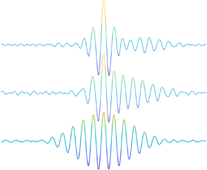
Figure 6(a) presents the measured average shape of the 20 largest crests at different locations in the numerical tank. The bandwidths at the different locations are  $\nu =\{0.12, 0.15, 0.18, 0.18, 0.18, 0.17\}$ corresponding to
  $x/\lambda _0=\{0, 10, 20, 30, 40, 50\}$. Figure 6(b) presents the linear predictions of these events at the same position based on the theory of quasi-determinism. The second-order bound harmonics are excluded in the figure, as the MNLS code computes the free wave directly without second-order bound harmonics. When generated, the group is symmetric and consistent with linear theory. As the waves evolve in space, the shape of the wave groups is modified by nonlinear physics. The main characteristics of this modification are a movement to the front of the wave group of the largest wave and a contraction of the wave group. We also present the shape of the crest profiles predicted by the theory of quasi-determinism (figure 6b). The changes in the predicted profiles in figure 6(b) are only due to changes in the wave spectrum with
  $x$ (cf. (
 $S(f,x)$ in (4.1)). Additionally, we present the averaged shape of the wave with the largest crest-to-trough height in appendix C.

Figure 6. Normalised average of (a) the 20 largest crest profiles out of over 6400 waves and (b) predicted crest profiles based on the theory of quasi-determinism at  $x/\lambda _0=0, 10 ,20, 30, 40, 50$ for random waves with a Gaussian input spectrum with
  ${\rm \Delta} f/f_0=0.054$ and
  $\epsilon =0.044$.
We quantify the changes to group shape using two parameters (following Tang, Tromans & Adcock Reference Tang, Tromans and Adcock2019). The first is a measure of the width of the group and the second a measure of the asymmetry. We begin by defining  $\sigma _1$ and
  $\sigma _2$ as the durations when the envelope height exceeds
  $80\,\%$ of the peak height of the envelope obtained by averaging the envelope corresponding to the 20 largest waves, where the envelope is obtained using a Hilbert transform. As illustrated in figure 7,
  $\sigma _1$ denotes the duration of the front flank of the group (passing the observer at earlier time) and
  $\sigma _2$ the duration of the rear flank (passing the observer at later time). We now define the parameters
  $B_1$ and
  $B_2$ to be the durations
  $\sigma _1$ and
  $\sigma _2$ as fractions of what would be predicted by linear theory from the local spectrum (i.e. from the theory of quasi-determinism):
 \begin{equation} B_{1} =\frac{\sigma_{1,{measured}} }{\sigma _{1,{quasi\text{-}determinism}}},\quad B_{2} =\frac{\sigma _{2,{measured}} }{\sigma_{2,{quasi\text{-}determinism}}}. \end{equation}
The ratios  $B_{1}$ and
  $B_{2}$ quantify the nonlinear modifications to both sides of the measured envelope shape compared to linear theory. We then define
  $B_{{mean}}$ and
  ${\rm \Delta} B$ as parameters respectively measuring changes in width and asymmetry relative to linear evolution:
 \begin{equation} B_{{mean}}=\frac{B_1+B_2}{2},\quad {\rm \Delta} B=B_2-B_1. \end{equation}
Thus, a positive value of  $1-B_{{mean}}$ implies the group has contracted relative to the shape expected under linear evolution. A positive value of
  ${\rm \Delta} B$ implies the largest wave has moved towards the front of the group.

Figure 7. Illustration of the envelope duration when the normalised envelope height  $|U|/|U|_{{max}}$ exceeds
  $80\,\%$ of its peak height.
Figure 8 presents the evolution of the parameters for asymmetry and change in group duration. Different initial bandwidth values are given in different panels with different lines for different steepnesses. In all cases, we observe a positive asymmetry, that is, the largest wave moves to the front of the group and arrives earlier. Spatially, the pattern is similar to that of kurtosis. For most cases, there is a peak in the asymmetry parameter during the initial phase before settling down to a smaller near-zero equilibrium value. As for kurtosis, the length scale for equilibrium to be reached is faster for narrower bandwidth. The degree of contraction of the wave group behaves differently. It increases steadily until it flattens off as equilibrium is achieved. The contraction occurs on a different, much longer, spatial scale from the transient asymmetry.

Figure 8. Group shape during nonlinear evolution in space: (a,c,e) envelope asymmetry ( ${\rm \Delta} B$) and (b,d,f) nonlinear change in the duration when the envelope height exceeds
  $80\,\%$ of its peak height (
 $1-B_{{mean}}$) with different initial bandwidths (a,b)
  ${\rm \Delta} f/f_0=0.054$, (c,d)
  ${\rm \Delta} f/f_0=0.09$ and (e,f)
  ${\rm \Delta} f/f_0=0.126$.
5. Discussion and conclusions
This paper has examined experimentally and numerically how the kurtosis and the shape of large waves evolve over relatively long distances for unidirectional surface gravity waves. In doing so, we have revisited the seminal unidirectional laboratory experiments of Onorato et al. (Reference Onorato, Osborne, Serio, Cavaleri, Brandini and Stansberg2004), which we repeat, extend and complement with numerical solutions of the fully nonlinear water wave equations and the MNLS of Trulsen et al. (Reference Trulsen, Kliakhandler, Dysthe and Velarde2000). We concentrate on the spatial evolution from a random boundary condition without correlation between components. Following nonlinear evolution, the kurtosis must eventually settle down to a steady state for unidirectional waves (without higher-order nonlinearity), in which changes to the spectrum no longer occur, and the kurtosis has a fixed value greater than that of a Gaussian ‘sea state’. We have investigated the transition between these two states and the dependence of the final state on the input conditions.
The picture we find is consistent across the different models and the different cases investigated. For the unidirectional cases studied here, we do not find any significant difference in overall behaviour between JONSWAP and Gaussian spectra, although we note that there is significant ambiguity when calculating the spectral bandwidth for the JONSWAP spectrum. For an input spectrum which is not too narrow-banded or steep (low BFI), theories based on either the NLS (Mori & Janssen Reference Mori and Janssen2006) or cDZ (Fedele & Dutykh Reference Fedele and Dutykh2012) are excellent models matching both experiments and simulations. However, if the input spectrum is steep or narrow, as captured by a high value of the BFI, the evolution of the excess kurtosis departs from these models. Significant changes occur to the spectrum over relatively short distances. Over the same short distances, excess kurtosis rapidly increases and peaks. The overshoot can be interpreted as being driven by the initial departure of phases from their equilibrium distribution (as can be seen by randomising the phases once steady state has been achieved). Over longer distances excess kurtosis then drops until it reaches a steady-state value with no further evolution of the spectrum. The peak and hence the final value are at a lower kurtosis than that predicted theoretically based on the NLS and cDZ. For cases which are sufficiently nonlinear to depart from the theoretical curve, the kurtosis at steady state appears to be primarily dependent on the initial bandwidth of the spectrum (rather than the steepness).
We note that Janssen (Reference Janssen2003) was already aware of the absence of an overshoot in his theoretical calculations based on the kinetic approach; these calculations based on the kinetic approach ultimately led to the result of Mori & Janssen (Reference Mori and Janssen2006) we have compared to herein. Janssen's (Reference Janssen2003) numerical simulations for the time evolution of spectral width show a similar overshoot to what we have observed for kurtosis (cf. his figure 3). This overshoot is also present in numerical simulations based on the NLS in Onorato et al. (Reference Onorato, Proment, El, Randoux and Suret2016) (their figure 1, where the overshoot is also present in bandwidth). This overshoot, Janssen (Reference Janssen2003) notes, is likely ignored in his theoretical calculations owing to the assumption that the action density varies slowly, an assumption which was later relaxed in the generalised kinetic equation of Annenkov & Shrira (Reference Annenkov and Shrira2006). In this paper we have examined a scenario where the spectrum undergoes a transient broadening at the location of the peaks in kurtosis. We thus envisage that calculations based on the generalised kinetic equation of Annenkov & Shrira (Reference Annenkov and Shrira2006) will predict the behaviour of kurtosis for steep and narrow-bandwidth spectra identified herein.
Examining simultaneously the effect of nonlinear evolution on shape of the largest waves, there is a tendency for the largest wave in a packet to move towards the front of the group. This asymmetry follows a similar path to the kurtosis, showing a clear peak during the early stage of evolution before reducing to become relatively small once equilibrium is reached. There is also a reduction in the width of an extreme event making the extreme event appear more transient. This follows a different evolution as it increases monotonically before reaching equilibrium on a longer spatial scale than the spatial scale associated with the asymmetry. The locations of the maxima of kurtosis coincide approximately with the locations of the maxima of asymmetry of the average shape of extreme events.
We conclude by emphasising that our paper is confined to unidirectional waves, so that its findings cannot directly be extended to real-world ocean waves, which are directionally spread. For directionally spread ocean waves, peaks in kurtosis also occur (Annenkov & Shrira Reference Annenkov and Shrira2009; Onorato et al. Reference Onorato, Cavaleri, Fouques, Gramstad, Janssen, Monbaliu, Osborne, Pakozdi, Serio and Toffoli2009; Toffoli et al. Reference Toffoli, Gramstad, Trulsen, Monbaliu, Bitner-Gregersen and Onorato2010; Xiao et al. Reference Xiao, Liu, Wu and Yue2013; Fedele Reference Fedele2015; Annenkov & Shrira Reference Annenkov and Shrira2018), yet as a result of very different underlying physics.
Acknowledgements
This work was funded by UK/China ORE funding (EPSRC/NERC/NSFC EP/R007632/1), the De-Risk project funded by Innovation Fund Denmark, the National Natural Science Foundation of China (51761135012 and 11872248) and the Ministry of Science and Technology of China (no. 2017YFE0132000). T.S.v.d.B. acknowledges a Royal Academy of Engineering Research Fellowship.
Declaration of interests
The authors report no conflict of interest.
Appendix A. Evolution of excess kurtosis
In this appendix, we explicitly provide the equations we use to evaluate the analytical solutions shown in figure 2.
A.1. The NLS (Mori & Janssen Reference Mori and Janssen2006)
Mori & Janssen (Reference Mori and Janssen2006) present the evolution of excess kurtosis for the time evolution of spatially homogeneous unidirectional waves that are initially normally distributed in the form of a three-dimensional integral (their (14)), which is subsequently evaluated in the narrow-bandwidth and large-time limit for Gaussian spectra (their (28)). Without taking the large-time limit, but invoking the other two solutions, this integral can be evaluated in closed form (Fedele et al. Reference Fedele, Cherneva, Tayfun and Guedes Soares2010) (see also Fedele Reference Fedele2015; Janssen & Janssen Reference Janssen and Janssen2019):
 \begin{equation} \frac{C^d_{4,{NLS}}(x)}{{BFI}^2}=\frac{\rm \pi}{3\sqrt{3}} \left[ 1-\frac{6}{\rm \pi}\textrm{Im}\left(i \arcsin{\frac{1+2i\alpha}{2}} \right)\right], \end{equation}
where  $C^d_{4,{NLS}}$ is the dynamic excess kurtosis based on the NLS,
  $\textrm {Im}$ is the imaginary part,
  $\alpha =2\nu ^2x/\lambda _0$ and
  $\nu$ is the bandwidth of the frequency spectrum. To obtain (A 1), we have also converted from time to space (see Fedele et al. Reference Fedele, Cherneva, Tayfun and Guedes Soares2010).
A.2. The cDZ (Fedele Reference Fedele2014)
Fedele (Reference Fedele2014) also proposes a correction of  $C^d_{4,{NLS}}$ based on the cDZ:
 \begin{equation} C_{4,{cDZ}}^{d}=C_{4,{NLS}}^{d}(1-0.4\nu_k^{2}).\end{equation}
 Here,  $\nu _k\approx 2\nu$ is the spectral bandwidth of the wavenumber spectrum
  $S(k)$ and
  $\nu$ that of the frequency spectrum
  $S(f)$. Then,
 \begin{equation} C_{4,{cDZ}}^{d}=C_{4,{NLS}}^{d}(1-1.6\nu^{2}),\end{equation}
for narrow-band waves (small  $\nu$).
We do not use the full model derived in Fedele (Reference Fedele2014), which is valid for waves evolving in time, but only the leading-order correction in bandwidth given here.
Appendix B. Figure with BFI at steady state
In figure 9 we show the same results as in figure 2 but with excess kurtosis normalised at steady state by BFI $_{ss}^2$. We thus obtain better agreement with theoretical results at large distances but worse agreement at small distances. Evidently, neither normalisation captures the occurrence of a maximum.

Figure 9. Evolution of normalised dynamic excess kurtosis at different distances from the wave generator: (a) case 1, (b) case 2 and (c) case 3. Shading represents the 95 % confidence intervals for OceanWave3D (OW3D) simulation with eight different random seeds. A total of 120 different random seeds are used in MNLS simulations. Consequently, for the MNLS, the error bars are negligible and have been omitted for clarity. The parameter  $C^d_4$ is dynamic excess kurtosis,
  $\textrm {BFI}_{ss}$ is the BFI at steady state,
  $\nu$ is the input bandwidth and
  $\lambda _0$ is the peak wavelength. This figure is equivalent to figure 2 except for the normalisation by the steady-state BFI (this figure) rather than the input BFI (figure 2).
Appendix C. Averaged shape of the wave with the largest crest-to-trough height
The theory of quasi-determinism predicts the shape of the wave with the largest crest-to-trough height as the scaled difference of two time-shifted auto-covariance functions (Boccotti Reference Boccotti1989, Reference Boccotti2000).
Figure 10(a) presents the average shape of the five largest crest-to-trough wave profiles at different locations. The general trend of the shape evolution is very similar to that of the largest crest events presented in figure 6. We also observe a movement of the largest crest to the front of the wave group and a contraction of the wave group for extreme crest-to-trough events. Figure 10(b) presents the predictions from the (linear) theory of quasi-determinism (Boccotti Reference Boccotti1989, Reference Boccotti2000). All the changes to the group shape in figure 10(b) are due to changes in the wave spectrum.

Figure 10. Average shape of the five largest crest-to-trough wave height profiles out of over 6400 waves profiles (a) and wave profiles predicted by the theory of quasi-determinism (b) at  $x/\lambda _0=0, 10 ,20, 30, 40, 50$ for random waves with a Gaussian input spectrum with
  ${\rm \Delta} f/f_0=0.054$ and
  $\epsilon =0.044$.


