2.1. The resolvent operator

Let us consider the Navier–Stokes equations in the general, spatially discretised form

(2.1)\begin{equation} \boldsymbol{\mathsf{G}}\,\frac{{\rm d} \boldsymbol{q}}{{\rm d}t}=\boldsymbol{\mathcal{N}}(\boldsymbol{q}), \end{equation}

where $\boldsymbol {q}$ is the spatially discretised state vector, and $\boldsymbol {\mathcal {N}}$ represents the right-hand side of the unforced Navier–Stokes equations. Including the mass-matrix $\boldsymbol{\mathsf{G}}$ in (2.1) means that this form could represent either the compressible Navier–Stokes equations or the incompressible equations where there is no time derivative in the continuity equation. By linearising this equation about a base-flow $\boldsymbol {q}_0$, we can write the system in input–output form as

(2.2)\begin{gather} \boldsymbol{\mathsf{G}}\,\frac{{\rm d} \boldsymbol{q}}{{\rm d}t}=\boldsymbol{\mathsf{L}}_{\boldsymbol{q}_0}\boldsymbol{q} + \boldsymbol{\mathsf{B}}\boldsymbol{f}, \end{gather}

(2.3)\begin{gather}\boldsymbol{y}=\boldsymbol{\mathsf{C}}\boldsymbol{q}, \end{gather}

where $\boldsymbol{\mathsf{L}}_{\boldsymbol {q}_0}$ is the linearised Navier–Stokes operator (Jeun, Nichols & Jovanović Reference Jeun, Nichols and Jovanović2016). The matrix $\boldsymbol{\mathsf{B}}$ allows for the introduced forcing $\boldsymbol {f}$ (input) to be windowed in space or restricted to specific equations or state variables. In an analogous manner, the matrix $\boldsymbol{\mathsf{C}}$ allows for a similar windowing to be applied to the output $\boldsymbol {y}$.

The relationship between harmonic inputs and outputs with frequency $\omega$ can be obtained by Laplace transforming the input–output system in time, giving the relation

(2.4)\begin{equation} \hat{\boldsymbol{y}}=\boldsymbol{\mathsf{C}}(-{\rm i}\omega\boldsymbol{\mathsf{G}}-\boldsymbol{\mathsf{L}}_{\boldsymbol{q}_0})^{{-}1}\boldsymbol{\mathsf{B}}\hat{\boldsymbol{f}}. \end{equation}

Through this equation, the resolvent operator is defined via $\boldsymbol {\mathcal {H}}_{\boldsymbol {q}_0} \equiv \boldsymbol{\mathsf{C}}(-{\rm i}\omega \boldsymbol{\mathsf{G}}-\boldsymbol{\mathsf{L}}_{\boldsymbol {q}_0})^{-1}\boldsymbol{\mathsf{B}}$. The form of (2.4) shows that the resolvent operator is equivalent to a transfer function that maps the forcing to its time-asymptotic response. Before we discuss the meaning of the resolvent in fluid dynamics, it is worth considering the Laplace variable $\omega$. If the operator $\boldsymbol{\mathsf{L}}_{\boldsymbol {q}_0}$ is stable, then $\omega$ is real and (2.4) is obtainable via the Fourier transform. However, if $\boldsymbol{\mathsf{L}}_{\boldsymbol {q}_0}$ is unstable, then more care is needed. Indeed, for unstable $\boldsymbol{\mathsf{L}}_{\boldsymbol {q}_0}$, the time-asymptotic response is not given via (2.4) and is instead a combination of the exponentially growing disturbance given by the most unstable eigenvector and the forced response given by the resolvent. In order to separate these two mechanisms, a complex value for $\omega$ can be used, leading to the concept of a time-discounted resolvent analysis (Jovanović Reference Jovanović2004). Choosing complex values for $\omega$ means that the imaginary part can be chosen such that the forced response ‘rises above’ the exponentially growing disturbance due to the unstable nature of $\boldsymbol{\mathsf{L}}_{\boldsymbol {q}_0}$, allowing for the forced dynamics to be probed (see Yeh et al. (Reference Yeh, Benton, Taira and Garmann2020) for more details).

In the context of fluid dynamics, the resolvent can be interpreted in two main ways. First, choosing $\boldsymbol {q}_0$ to be a steady solution of the unforced Navier–Stokes equations leads to a non-normal stability study of the flow. In this manner, the resolvent identifies forcing structures that lead to particularly efficient amplification in the dynamics despite the stable nature of the flow (Trefethen et al. Reference Trefethen, Trefethen, Reddy and Driscoll1993). Second, using a time-averaged mean-flow for $\boldsymbol {q}_0$ leads to the resolvent formulation of turbulence (McKeon & Sharma Reference McKeon and Sharma2010). The resolvent in this instance can be used to identify the coherent structures that arise via disturbances caused by the nonlinear terms.

For both steady base-flows and time-averaged mean-flows, the resolvent provides critical insights into how forcings can cause an amplification in the dynamics. This amplification can occur both from resonant frequencies and also from particularly effective structural mechanisms. Whilst one could choose a variety of forcings $\hat {\boldsymbol {f}}$ at each frequency to determine the most effective structures, it is more efficient to solve directly for the optimal forcing. This can be formulated mathematically as

(2.5)\begin{equation} \boldsymbol{f}_{opt}=\underset{\boldsymbol{f}}{\text{arg max}}\, \frac{\|\boldsymbol{y}\|_{\boldsymbol{\mathsf{W}}_{\boldsymbol{q}}}}{\|\boldsymbol{f}\|_{\boldsymbol{\mathsf{W}}_{\boldsymbol{f}}}}, \end{equation}

where the norms are defined as $\|\boldsymbol { a}\|^{2}_\boldsymbol{\mathsf{W}}=\boldsymbol {a}^{H}\boldsymbol{\mathsf{W}}\boldsymbol {a}$, with $\boldsymbol{\mathsf{W}}$ being a positive definite weight matrix. We allow for the weight matrices for the forcing ($\boldsymbol{\mathsf{W}}_{\boldsymbol {f}}$) and response ($\boldsymbol{\mathsf{W}}_{\boldsymbol {q}}$) to be different. These matrices are problem-dependent, and are chosen so that the norms represent appropriate measures of the energy (see §§ 3.1 and 3.2 for examples). The cost functional in this case is the gain. To link the weighted norms to the two norms, it is useful to also consider the Cholesky decomposition $\boldsymbol{\mathsf{W}}=\boldsymbol{\mathsf{M}}^{H}\boldsymbol{\mathsf{M}}$. The optimal forcing has the corresponding output $\tilde {\boldsymbol {y}}_{opt}=\boldsymbol {\mathcal {H}}\boldsymbol {f}_{opt}$, with the amount of amplification being measured by the gain $\sigma =\|\tilde {\boldsymbol {y}}_{opt}\|_{\boldsymbol{\mathsf{W}}_{\boldsymbol {q}}}/\|\boldsymbol {f}_{opt}\|_{\boldsymbol{\mathsf{W}}_{\boldsymbol {f}}}$. This problem can be solved by taking the singular value decomposition (SVD) of $\boldsymbol{\mathsf{M}}_{\boldsymbol {q}}\boldsymbol {\mathcal {H}}\boldsymbol{\mathsf{M}}_{\boldsymbol {f}}^{-1}$, whose maximum singular triplet is $(\sigma,\boldsymbol{\mathsf{M}}_{\boldsymbol {q}}\boldsymbol {y}_{opt},\boldsymbol{\mathsf{M}}_{\boldsymbol {f}}\boldsymbol {f}_{opt})$.

While a resolvent analysis in this manner can provide useful information about frequencies and forcing structures that can provide a large amplification, and therefore identify good candidates for flow control, the forcing structures are often global. This means that implementing them in a practical situation is infeasible. In the present study, we present an approach to finding sparse (spatially compact) resolvent forcings that induce large amplifications in the underlying dynamics. In this manner, particularly sensitive spatial locations in the flow field are identified, providing a guide for effective and efficient actuation.

2.2. Sparsification via Riemannian optimisation

To seek a spatially sparse resolvent forcing mode, we first generalise the optimal forcing problem. We start by realising that finding the greatest singular value of the resolvent matrix is equivalent to maximising the gain

(2.6)\begin{equation} \sigma=\frac{\|\boldsymbol{\mathcal{H}}\boldsymbol{f}\|^{2}_{\boldsymbol{\mathsf{W}}_{\boldsymbol{q}}}}{\|\boldsymbol{f}\|^{2}_{\boldsymbol{\mathsf{W}}_{\boldsymbol{f}}}}. \end{equation}

Therefore, instead of carrying out an SVD, we could instead maximise the gain via a gradient ascent algorithm. It is useful to phrase this optimisation as follows: maximise the gain

(2.7)\begin{equation} \sigma=\|\boldsymbol{\mathcal{H}}\boldsymbol{f}\|^{2}_{\boldsymbol{\mathsf{W}}_{\boldsymbol{q}}}, \end{equation}

where the forcing is confined to the manifold given by the constraint $\|\boldsymbol {f}\|^{2}_{\boldsymbol{\mathsf{W}}_{\boldsymbol {f}}}=1$. This problem is equivalent to (2.6) because the resolvent is linear and hence will produce the same gain defined by (2.6) if we choose the forcing to have a unit-energy norm. In effect, by constraining our forcing to this manifold, we are ensuring that we search for the maximum amplification in dynamics with the forcing having the same energy budget.

Whilst we could conduct an unconstrained optimisation by enforcing $\|\boldsymbol {f}\|_{\boldsymbol{\mathsf{W}}_{\boldsymbol {f}}}^{2}=1$ with a Lagrange multiplier (Pringle, Willis & Kerswell Reference Pringle, Willis and Kerswell2012), we instead take account of this constraint directly in the update step. This results in an approach similar to that of Foures et al. (Reference Foures, Caulfield and Schmid2013), where a geometric approach (Douglas, Amari & Kung Reference Douglas, Amari and Kung1998) was used to ensure that the unit-norm condition is satisfied when stepping in the search direction. In general, carrying out an optimisation where the input is constrained to a manifold is known as Riemannian optimisation (Absil, Mahony & Sepulchre Reference Absil, Mahony and Sepulchre2007).

Let us first discuss the optimisation problem considered thus far. We seek to maximise the gain

(2.8)\begin{equation} \sigma^{(L_2)}=\|\boldsymbol{\mathsf{M}}_{\boldsymbol{q}}\boldsymbol{\mathcal{H}}\boldsymbol{\mathsf{M}}_{\boldsymbol{f}}^{{-}1}\boldsymbol{\mathsf{M}}_{\boldsymbol{f}}\boldsymbol{f}\|_2, \end{equation}

subject to $\|\boldsymbol{\mathsf{M}}_{\boldsymbol {f}}\boldsymbol {f}\|_2=1$. By expressing the problem in this form, we have reformulated the problem in terms of the $L_2$-norm, hence we are optimising with respect to the vector $\boldsymbol {f}_\boldsymbol{\mathsf{M}}=\boldsymbol{\mathsf{M}}_{\boldsymbol {f}}\boldsymbol {f}$, which we constrain to have unit $L_2$-norm. The manifold for this problem then becomes the complex hypersphere $\mathcal {S}=\{\boldsymbol {y}\,|\,\boldsymbol {y}^{H}\boldsymbol {y}=1\}$.

For an unconstrained optimisation, we generally work with the Euclidean gradient

(2.9)\begin{equation} \boldsymbol{\nabla}_{\boldsymbol{f}_\boldsymbol{\mathsf{M}}} \sigma^{(L_2)}=\frac{\partial \sigma^{(L_2)}}{\partial \boldsymbol{f}_\boldsymbol{\mathsf{M}}}. \end{equation}

By stepping in the direction of the conjugate of this gradient, we would be increasing the value of $\sigma ^{(L_2)}$, assuming that we use a sufficiently small step size for which a linear approximation is appropriate. The problem with this approach is that stepping in such a direction would most likely result in a vector that is no longer on the manifold.

To carry out a gradient descent on the hypersphere, we must therefore define the gradients appropriately. Riemannian optimisation will not work directly with the Euclidean gradient, but instead all gradients must be tangent to the hypersphere at the evaluation points. The set of all vectors tangent to the manifold at a point $\boldsymbol {x}$ is known as the tangent space ${T}_{\boldsymbol {x}}\mathcal {S}$, with the set of all tangent spaces being referred to as the tangent bundle ${T}\boldsymbol {x}=\sum _{\boldsymbol {x}\in \mathcal {S}}{T}_{\boldsymbol {x}}\mathcal {S}$ (see figure 1, which shows schematically the Riemannian optimisation procedure). For the hypersphere, the Riemannian gradient can be written as

(2.10)\begin{equation} \text{grad}\,\sigma^{(L_2)}(\boldsymbol{f}_\boldsymbol{\mathsf{M}}) = \boldsymbol{\nabla}_{\boldsymbol{f}_\boldsymbol{\mathsf{M}}}\sigma^{(L_2)} - \left(\boldsymbol{f}_\boldsymbol{\mathsf{M}}^{H}\, \boldsymbol{\nabla}_{\boldsymbol{f}_\boldsymbol{\mathsf{M}}} \sigma^{(L_2)}\right) \boldsymbol{f}_\boldsymbol{\mathsf{M}} = \text{Proj}_{\boldsymbol{f}_\boldsymbol{\mathsf{M}}}\left(\boldsymbol{\nabla}_{\boldsymbol{f}_\boldsymbol{\mathsf{M}}} \sigma^{(L_2)}\right), \end{equation}

where the function $\text {Proj}$ is the projection that links the Riemannian gradient to the Euclidean one.

Figure 1. A sketch illustrating the concept of Riemannian optimisation. First, the Euclidean gradient $\boldsymbol {\nabla }_{\boldsymbol {f}^{n}_\boldsymbol{\mathsf{M}}} \sigma ^{(L_2)}$ is found from the vector $\boldsymbol {f}^{n}_\boldsymbol{\mathsf{M}}$ that is situated on the hypersphere $\mathcal {S}$. This vector is then mapped to the tangent space $T_{\boldsymbol {f}^{n}_\boldsymbol{\mathsf{M}}}\mathcal {S}$ via the projection $\text {Proj}_{\boldsymbol {f}^{n}_\boldsymbol{\mathsf{M}}}$. Next, the Riemannian gradient is extended along the tangent space by the step size $\alpha$. Finally, we map this gradient back to the manifold via the retraction $R_{\boldsymbol {f}^{n}_\boldsymbol{\mathsf{M}}}$, yielding the updated forcing vector $\boldsymbol {f}^{n+1}_\boldsymbol{\mathsf{M}}$. For varying values of $\alpha$, the retraction traces out a smooth curve over the manifold, displayed as a dotted line. The link between $\alpha$ and $\theta$ is also shown.

Now that we have defined appropriate gradients, we must also define how to step in the direction of steepest ascent. For the unconstrained optimisation, we may simply add a scalar multiple (the step size) of this gradient onto our current value of the forcing. However, for the Riemannian optimisation, this will result in a vector that no longer falls on the manifold, as noted above. The equivalent procedure in this case is the notion of a retraction. A retraction is a mapping $R_{\boldsymbol {x}}(\boldsymbol {\xi }):{T}_{\boldsymbol {x}}\mathcal {S}\rightarrow \mathcal {S}$ such that $R_{\boldsymbol {x}}({\bf 0})=\boldsymbol {x}$ and ${\rm D}R_{\boldsymbol {x}}({\bf 0})=\text {id}_{{{T}_{\boldsymbol {x}}\mathcal {S}}}$. In other words, a retraction maps vectors tangent to the manifold at $\boldsymbol {x}$ to other vectors on the manifold such that for $\boldsymbol {\xi }=\boldsymbol {0}$ it maps $\boldsymbol {x}$ to itself, and such that the derivative of the mapping at $\boldsymbol {\xi }=\boldsymbol {0}$ is the identity. For the hypersphere, we have the retraction

(2.11)\begin{equation} R_{\boldsymbol{x}}(\boldsymbol{\xi})=\frac{\boldsymbol{x}+\boldsymbol{\xi}}{\|\boldsymbol{x}+\boldsymbol{\xi}\|}. \end{equation}

Once the gradient is found, we can then update the forcing using the map $R_{\boldsymbol {f}_\boldsymbol{\mathsf{M}}} \left (\alpha \,\text {grad}\, \sigma ^{(L_2)} (\boldsymbol {f}_\boldsymbol{\mathsf{M}})\right )$, where $\alpha$ denotes the step size. By writing $\cos (\theta )=1/\sqrt {1+\alpha ^{2}}$, we can also express the update step as

(2.12)\begin{equation} \boldsymbol{f}_\boldsymbol{\mathsf{M}}^{n+1} =R_{\boldsymbol{f}_\boldsymbol{\mathsf{M}}^{n}}\left(\alpha\,\text{grad}\, \sigma^{(L_2)}(\boldsymbol{f}_\boldsymbol{\mathsf{M}}^{n})\right)=\cos(\theta)\,\boldsymbol{f}_\boldsymbol{\mathsf{M}}^{n} +\sin(\theta)\,\text{grad}\, \sigma^{(L_2)}(\boldsymbol{f}_\boldsymbol{\mathsf{M}}^{n}), \end{equation}

which is exactly the geometric form used by Foures et al. (Reference Foures, Caulfield and Schmid2013). Note that we have described a steepest ascent approach here. However, many alternative gradient-based optimisation algorithms, such as the conjugate gradient and Broyden–Fletcher–Goldfarb–Shanno (BFGS) algorithms, are applicable to Riemannian optimisation with faster convergence (Boumal & Absil Reference Boumal and Absil2015; Huang, Absil & Gallivan Reference Huang, Absil and Gallivan2016).

The main advantage of phrasing the optimal forcing output problem in this way is its generality. Whilst we have shown how we can obtain the same result as the SVD (and it is actually possible to get the higher-order singular values in this manner by considering a different manifold), we are free to change how we define the gain. The SVD can find the gain only in the $L_2$-norm sense. This means that the input is measured by an energy norm, leading to the global structures seen in many studies. In order to introduce sparsification, we consider the use of the 1-norm.

A sketch of the unit $L_2$- and $L_1$-norms for a vector $(x,y)$ in ${\mathbb {R}}^{2}$ is presented in figure 2(a). The $L_2$-norm takes the form of a circle, whereas the $L_1$-norm yields a regular diamond inscribed within this circle. Note that the unit $L_1$-norm touches the unit $L_2$-norm at the coordinate axes. This indicates that the $L_1$-norm for all vectors with unit $L_2$-norm yields its smallest value for sparse vectors, i.e. vectors $(x,y)$ with either $x$ or $y$ equal to zero. Indeed, if the diamond touched the circle at another location $(x_0,y_0)$ with $x_0\neq 0$ and $y_0\neq 0$, then the $L_2$-norm would be unity whereas the $L_1$-norm would have the value $|x_0|+|y_0|>1$. Hence optimising over the space of unit-norm forcings, whilst penalising the $L_1$-norm, will push the forcing vector, and hence its structure, towards more locally supported structures.

Figure 2. Sketches of the $L_2$- and $L_1$-norms. The effect of a coordinate rotation on the norms is also demonstrated. (a) The unit $L_2$-norm (circle) and $L_1$-norm (diamond) with respect to the coordinate system $(x,y)$. (b) The $L_2$-norm (green dashed circle) and $L_1$-norm (green dashed square) with respect to the coordinate system $(\xi,\eta )$.

One important consideration when using an alternative norm, such as the $L_1$-norm, is illustrated by figure 2(b). Here, we have again shown the unit $L_2$- and $L_1$-norms, but this time for the coordinate system $(\eta,\xi )$ that is obtained via a rotation of the coordinate system $(x,y)$ by an angle $\theta$. In this new coordinate system, the $L_2$-norm still represents a circle, which is invariant under this transformation. However, the unit $L_1$-norm is affected, and its square shape is rotated by the angle $\theta$. This means that in this new coordinate system, the sparse vectors, where the square touches the circle, are different to those of the original coordinate system $(x,y)$. In other words, what is considered sparse is defined completely by how we choose to represent our vectors. In practice, we must be careful when choosing the vector of which we take the $L_1$-norm. We therefore choose to take the $L_1$-norm of a vector that leaves the $L_2$-norm unchanged, yet has appropriate axes for best defining the sparsity that we aim to achieve. In terms of resolvent analysis, this transformation is used to maintain the physical relevance of the sparsification. Specific examples are described in §§ 3.1 and 3.2.

Based on the discussion of the previous two paragraphs, we seek to maximise the new gain $\sigma ^{(L_1)}$ defined by

(2.13)\begin{equation} \sigma^{(L_1)}=\frac{ \sigma^{(L_2)}}{\|\boldsymbol{T}(\boldsymbol{f}_{\boldsymbol{\mathsf{M}}})\|_1} =\frac{\|\boldsymbol{\mathsf{M}}_{\boldsymbol{q}}\boldsymbol{\mathcal{H}}\boldsymbol{\mathsf{M}}_{\boldsymbol{f}}^{{-}1}\boldsymbol{f}_\boldsymbol{\mathsf{M}}\|_2}{\|\boldsymbol{T}(\boldsymbol{f}_{\boldsymbol{\mathsf{M}}})\|_1}, \end{equation}

still subject to the forcing $\boldsymbol {f}_\boldsymbol{\mathsf{M}}$ having a unit-energy norm. The transformation $\boldsymbol {T}$ in the denominator is a transformation of the vector $\boldsymbol {f}_\boldsymbol{\mathsf{M}}$ to another vector. Hence the vector in the denominator need not be equal to the forcing vector $\boldsymbol {f}_{\boldsymbol{\mathsf{M}}}$ as, based on the discussion of the previous paragraph, this may not be relevant physically. However, by ensuring $\|\boldsymbol {T}(\boldsymbol {f}_\boldsymbol{\mathsf{M}})\|_2=\|\boldsymbol {f}_\boldsymbol{\mathsf{M}}\|_2$, we maintain the geometric interpretation of sparsity illustrated by figure 2(a), albeit in a much higher-dimensional space. By dividing the usual gain by the 1-norm of the vector $\boldsymbol {T}(\boldsymbol {f}_\boldsymbol{\mathsf{M}})$, we are in effect promoting sparsity, with sparsity defined as a vector $\boldsymbol {T}(\boldsymbol {f}_\boldsymbol{\mathsf{M}})$ with a minimal number of non-zero entries. Optimising the gain in this form will seek a compromise between providing a large gain in energy whilst ensuring the spatial sparsity of the forcing. Indeed, the maximal nature of $\sigma ^{(L_1)}$ means that obtaining a response with larger energy requires a forcing structure that is less sparse. Likewise, making the forcing more sparse leads to a less energetic response.

As in the study of Foures et al. (Reference Foures, Caulfield and Schmid2013), who considered a similar optimisation problem for localising flow structures obtained in transient growth studies, our cost functional is non-convex. This means that any solution to the optimisation problem is guaranteed only to be a local, rather than global, maximum of the cost functional. In the case of transient growth, this led to multiple branches of solutions being found during the optimisation, which could be discovered by running the problem with multiple starting guesses for the gradient-based optimisation. However, despite running multiple instances of each optimisation with different initial guesses in our examples, no differences in the solution could be found apart from symmetries of the flow, which are to be expected. Whist this does not confirm that our results are truly the global optimum, it does highlight a difference between localising forcings for driven versus initial-condition based studies.

Another important factor is the realisation that the $L_1$-norm is notoriously hard to optimise due to its non-smoothness near the origin. Intuitively, we can visualise the problem by considering the unconstrained optimisation problem of minimising the $L_1$-norm of a scalar $a$. Using our gradient-based approach, this amounts to stepping in the direction of steepest descent, which for our simple example is the sign of $a$. No matter how near or far we are to the optimal value of $a=0$, this gradient will have the same magnitude. This means that we will step continuously over the optimal value, unless the step size is perfect, leading to zig-zagging and ultimately causing the algorithm to converge rather slowly. To alleviate this behaviour we replace the $L_1$-norm with a smooth approximation, namely $l_{1,\delta }(\boldsymbol {q}) = h_\delta (\boldsymbol {q})/\delta$, where $h_\delta (\boldsymbol {q})$ is the pseudo-Huber-norm (Bube & Langan Reference Bube and Langan1997; Bube & Nemeth Reference Bube and Nemeth2007)

(2.14)\begin{equation} h_\delta(\boldsymbol{q}) = \sum_j \delta^{2}\left(\sqrt{1+\frac{|q_j|^{2}}{\delta^{2}}}-1\right). \end{equation}

This pseudo-Huber-norm has the property that it approximates the $L_1$-norm for small $\delta$ and is completely smooth. Therefore, in order to achieve convergence, we will not optimise $\sigma ^{(L_1)}$ directly but perform a series of optimisations for the quantity

(2.15)\begin{equation} \sigma^{(L_1)}_\delta=\frac{\|\boldsymbol{\mathsf{M}}_{\boldsymbol{q}}\boldsymbol{\mathcal{H}}\boldsymbol{\mathsf{M}}_{\boldsymbol{f}}^{{-}1}\boldsymbol{f}_\boldsymbol{\mathsf{M}}\|_2}{l_{1,\delta}(\boldsymbol{T}(\boldsymbol{f}_\boldsymbol{\mathsf{M}}))}, \end{equation}

for decreasing values of $\delta$. By using the optimal forcing obtained from an optimisation for the preceding one with a lower value of $\delta$, we are able to achieve more robustly a converged optimisation for a sufficiently small $\delta$ such that our norm (2.14) is an appropriate approximation for the true $L_1$-norm.

Before concluding this section, it is important to note that our choice of cost functional is not unique. Indeed, other cost functionals such as $\sigma ^{(L_1)}=\sigma ^{(L_2)}-\mu \|\boldsymbol {T}(\boldsymbol {f}_\boldsymbol{\mathsf{M}})\|_1$ can also lead to sparse forcing modes for appropriate choices of $\mu$. However, the fact that unit-norm forcings can lead to gains in energy many orders of magnitude larger than that of the forcing makes the choice of $\mu$, which must balance the $L_2$-based gain against the $L_1$-based forcing, a difficult challenge. This is complicated further by the strong dependence of the gain on the forcing frequency, making a universally good way of choosing $\mu$ hard to determine. In our proposed cost functional there is no such parameter to choose, meaning that it can be applied easily to different frequencies and base-flows without change. Hence we continue with it for the rest of the study.

2.3. Resolvent wavemaker

One concept that we use in our subsequent analysis is that of structural sensitivity and the wavemaker (Giannetti & Luchini Reference Giannetti and Luchini2007). The wavemaker has its origin in global stability analysis and provides a way to highlight regions in which flow field changes result in changes to global modes. Specifically, the wavemaker is the structural sensitivity to a localised flow feedback. To obtain the wavemaker, we consider the eigenvalue problem $\boldsymbol{\mathsf{L}}\boldsymbol {x}=\lambda \boldsymbol{\mathsf{G}}\boldsymbol {x}$. This eigenvalue problem could arise, for instance, as a global stability problem, in which case $\boldsymbol {x}$ would be the global mode, with the corresponding eigenvalue $\lambda$ giving its frequency and growth rate. It can be shown (see the review of Schmid & Brandt (Reference Schmid and Brandt2014), for example) that to first order, a perturbation to the eigenvalue $\delta \lambda$ for a perturbation in the matrix $\boldsymbol {\delta } \boldsymbol{\mathsf{L}}$ is given via

(2.16)\begin{equation} \delta \lambda = \frac{\langle \boldsymbol{x}^{{{\dagger}}},\boldsymbol{\delta} \boldsymbol{\mathsf{L}} \boldsymbol{x}\rangle}{\langle \boldsymbol{x}^{{{\dagger}}},\boldsymbol{\mathsf{G}}\boldsymbol{x}\rangle}, \end{equation}

where $\boldsymbol {x}^{{\dagger} }$ is the solution to the adjoint eigenvalue problem $\boldsymbol{\mathsf{L}}^{H}\boldsymbol {x}^{{\dagger} }=\bar {\lambda } \boldsymbol{\mathsf{G}}^{H}\boldsymbol {x}^{{\dagger} }$. The wavemaker is then obtained by specifying $\boldsymbol {\delta } \boldsymbol{\mathsf{L}}=\boldsymbol{\mathsf{I}}$ and instead taking the elementwise, or Hadamard ($\odot$), product:

(2.17)\begin{equation} \boldsymbol{\lambda} = \frac{\bar{\boldsymbol{x}}^{{{\dagger}}}\odot \boldsymbol{x}}{\langle \boldsymbol{x}^{{{\dagger}}},\boldsymbol{\mathsf{G}}\boldsymbol{x}\rangle}. \end{equation}

In this way, the wavemaker $\boldsymbol {\lambda }$ can then be thought of as a vector field $\boldsymbol {\lambda }(x,y)=(\lambda _u,\lambda _v,\lambda _w)$ whose components represent what changes to the eigenvalue occur from localised feedback at each location and state component in the flow field.

We note quickly that there are a few ways in which the wavemaker could be perceived. Whilst we have stayed within a discrete setting, Giannetti & Luchini (Reference Giannetti and Luchini2007) present the wavemaker in a continuous formulation. This gives the main difference that their wavemaker is a scalar field that is defined pointwise via $\lambda (x,y)=\|\boldsymbol {x}^{{\dagger} }(x,y)\|\|\boldsymbol {x}(x,y)\|$. Hence their wavemaker, by the Cauchy–Schwarz inequality, shows the maximum change to the eigenvalue that can be achieved via localised feedback at each spatial location. Conversely, the wavemaker presented by Schmid & Brandt (Reference Schmid and Brandt2014) is more easily related to ours via $\lambda (x,y)=\lambda _u+\lambda _v+\lambda _w$. In this manner, they obtain a complex-valued wavemaker whose real and imaginary parts show the individual changes to the real and imaginary parts of the eigenvalue. Additionally, the sign of these changes is retained, allowing for the direction of the eigenvalue perturbation to be determined. However, by keeping the values of the flow field separate, our wavemaker definition is strongly related to that of Paladini et al. (Reference Paladini, Beneddine, Dandois, Sipp and Robinet2019), who introduce windowing matrices to allow for the selection of specific physical components in the resulting wavemaker. Whilst they use these matrices to isolate the contribution of the momentum to the wavemaker, we instead do this procedure for each separate velocity component. This means that for each spatial location, our wavemaker tells us how a specific eigenvalue will move for localised feedback restricted to each component of the state vector.

Whilst the previous paragraph talked about a wavemaker in terms of an eigenvalue problem, it can also be directly formulated for an SVD-based resolvent analysis (Qadri & Schmid Reference Qadri and Schmid2017). Indeed, by realising that taking the SVD of the matrix $\boldsymbol{\mathsf{K}}=\boldsymbol{\mathsf{M}}_{\boldsymbol {q}}\boldsymbol {\mathcal {H}}\boldsymbol{\mathsf{M}}_{\boldsymbol {f}}^{-1}$ is equivalent to taking the eigenvalues of the matrix $\boldsymbol{\mathsf{K}}^{H}\boldsymbol{\mathsf{K}}$, the same procedure that yields (2.16) can be applied, resulting in

(2.18)\begin{equation} \delta \sigma = \sigma^{2}\,\textrm{Re} \left(\langle \boldsymbol{f},\boldsymbol{\delta} \boldsymbol{\mathsf{L}} \boldsymbol{q}\rangle_{\boldsymbol{\mathsf{W}}_{\boldsymbol{f}}}\right), \end{equation}

where $\boldsymbol{\mathsf{L}}$ stands for the linearised Navier–Stokes operator (Fosas de Pando, Schmid & Lele Reference Fosas de Pando, Schmid and Lele2014; Fosas de Pando & Schmid Reference Fosas de Pando and Schmid2017; Qadri & Schmid Reference Qadri and Schmid2017). Again, taking $\boldsymbol {\delta }\boldsymbol{\mathsf{L}}=\boldsymbol{\mathsf{I}}$ and using the Hadamard product yields

(2.19)\begin{equation} \boldsymbol{\sigma} = \sigma^{2}\,\textrm{Re}\left(\bar{\boldsymbol{f}}\odot \boldsymbol{\mathsf{W}}_{\boldsymbol{f}} \boldsymbol{q}\right). \end{equation}

The resolvent wavemaker $\boldsymbol {\sigma }$ is then analogous to the eigenvalue-based wavemaker, i.e. for localised feedback at each spatial location and component of the state vector, the resolvent wavemaker will indicate how the singular value will be perturbed.

An example of the wavemaker and resolvent wavemaker is shown for cylinder flow in figure 3. It is important to note that for the eigenvalue-based wavemaker, the frequency is set by the eigenvalues. However, our definition of the resolvent wavemaker allows any frequency to be specified. Therefore, we concentrate on ${St}=0.162$, which is the frequency at which the most unstable eigenvalue is found. We observe that these wavemakers have similar structures but with different gains. The fact that they have similar structures is not surprising, since the resolvent forcing and response modes are similar qualitatively to the direct and adjoint eigenvectors, respectively. However, the signs of the structures are often different. This indicates that a localised feedback affects the eigenvalue perturbation differently from the singular value perturbation, highlighting the importance of formulating a resolvent wavemaker in order to quantify the effect of localised feedback for resolvent analyses.

Figure 3. The eigenvalue-based wavemakers and resolvent wavemakers for cylinder flow at $Re=100$ shown for illustration. Computations are performed with the immersed boundary projection method ibmos (Fosas de Pando Reference Fosas de Pando2020). (a) Wavemaker for the real part of the $u$-component. (b) Wavemaker for the real part of the $v$-component. (c) Resolvent wavemaker for the $u$-component at $St=0.162$. (d) Resolvent wavemaker for the $v$-component at ${St}=0.162$.

3.1. Plane Poiseuille flow

First, we consider plane Poiseuille flow to compare the differences in localisation strategies between initial-condition-based (transient growth) and driven (resolvent) studies. The present set-up follows that of Foures et al. (Reference Foures, Caulfield and Schmid2013) in which a domain covers $(x,y)\in [0,2{\rm \pi} ]\times [0,2]$ at Reynolds number ${Re}=4000$. No-slip boundary conditions are applied at $y=0$ and $2$, and periodic boundary conditions are applied at $x=0$ and $2{\rm \pi}$. The base-flow is provided analytically as $u=y(2-y)$. We conduct the numerical simulations using the Python package ibmos developed by Fosas de Pando (Reference Fosas de Pando2020). This is an immersed boundary projection code based on the formulation of Taira & Colonius (Reference Taira and Colonius2007) with specific formulation for optimisation and stability analyses. The package solves the nonlinear incompressible Navier–Stokes equations and provides directly the linearised and adjoint codes necessary for conducting a resolvent analysis. For the plane Poiseuille examples, the matrix $\boldsymbol{\mathsf{B}}$ is chosen so that the forcing is added to only the momentum equations. Similarly, the matrix $\boldsymbol{\mathsf{C}}$ is chosen so that only velocity components constitute the output.

As detailed in § 2.2, there is some consideration in choosing the vector for our $L_1$-norm, $\boldsymbol {T}(\boldsymbol {f}_\boldsymbol{\mathsf{M}})$. The obvious choice would be to use the same vector used for the unit-energy norm, ${\boldsymbol {f}}_{\boldsymbol{\mathsf{M}}}$, for the $L_1$-norm. However, as the $x$- and $y$-components of the velocity occur in different locations of ${\boldsymbol {f}}_{\boldsymbol{\mathsf{M}}}$, this would result in a sparsification that not only sparsifies the forcing mode in space, but also sparsifies between the $x$- and $y$-components of velocity. In other words, if the sparse procedure were to locate a single spatial point for the forcing mode, then it would also be advantageous to align the velocity vector completely with the coordinate axes at this point, in order to achieve a further reduction in the $L_1$-norm. As we are interested primarily in localisation in space, as opposed to sparsifying the velocity vector itself, we therefore design a vector for the $L_1$-norm optimisation that does not result in this unwanted sparsification. This is particularly pertinent to applications of this method to flow-actuation, where the directional information obtained by keeping the $x$-, $y$- and possibly $z$-components of velocity independent of the sparsification procedure will provide additional insight into actuator design.

To this end, we consider a vector of the form $\boldsymbol {T}(\boldsymbol {f}_\boldsymbol{\mathsf{M}})=\boldsymbol{\mathsf{M}}(\boldsymbol {u}\odot \boldsymbol {u}+\boldsymbol {v}\odot \boldsymbol {v})^{1/2}$, where $\odot$ is the Hadamard product, and the square root is taken componentwise. This vector has the same 2-norm as ${\boldsymbol {f}}_{\boldsymbol{\mathsf{M}}}$, but groups local contributions of the forcing mode to the total energy together. Hence the $L_1$-norm of this vector is small when the forcing is localised in space, but without penalising among individual components of the velocity vector. It should be noted that some additional care may be needed when designing this vector, depending on the specific numerical implementation. For example, as our immersed boundary implementation uses a staggered mesh with the $x$-components of velocity lying on the east and west faces of the cell whilst the $y$-components lie on the north and south faces, we form the vector $\boldsymbol {T}(\boldsymbol {f}_\boldsymbol{\mathsf{M}})$ on the cell centres by averaging the kinetic energy contributions from the cell edges. The weight matrices are chosen to incorporate the grid spacing (see Taira & Colonius (Reference Taira and Colonius2007) for more information), so that the forcing and response are measured in terms of the kinetic energy.

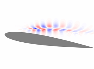
3.2. Flow past an aerofoil

Next, we also consider a spanwise-periodic turbulent flow over a canonical aerofoil obtained from a large-eddy simulation (LES) with a Vremen subgrid scale model (Vreman Reference Vreman2004). The LES is conducted using the finite-volume solver CharLES that solves the compressible Navier–Stokes equations with second-order spatial and third-order temporal accuracies (Khalighi et al. Reference Khalighi, Nichols, Ham, Lele and Moin2011; Brès et al. Reference Brès, Ham, Nichols and Lele2017). The linearisation is performed within the same solver (Sun et al. Reference Sun, Taira, Cattafesta and Ukeiley2017), considering the time- and spanwise-averaged turbulent flow over the aerofoil as the base-flow.

The resolvent analysis is performed on a mesh separate from that used by the LES. The mesh for the resolvent analysis has a two-dimensional rectangular domain of extent $x/L_c \in [-15, 16]$ and $y/L_c \in [-6, 5]$, comprising approximately $0.11$ million cells and giving the resulting discretised linear operator dimension $540\,840 \times 540\,840$. Compared to the LES mesh, the mesh for resolvent analysis is coarser over the aerofoil and in the wake, but is much finer in the upstream region of the aerofoil in order to resolve the forcing mode structures. The convergence of resolvent norm with respect to the domain extent and grid resolution has been reported in detail in Yeh & Taira (Reference Yeh and Taira2019). At the far-field boundary and over the aerofoil, Dirichlet conditions are specified for the density and velocities, and Neumann conditions are prescribed for the pressure in $\boldsymbol {q}$. At the outlet boundary, Neumann conditions are provided for all flow variables. The base-flow is two-dimensional, however, in contrast to the plane Poiseuille case, and we allow the perturbations to be three-dimensional by adopting a bi-global setting that decomposes $\boldsymbol {q}$ into spanwise Fourier modes with wavenumber $\beta$.

Even though the linear operator is sparse, its large dimension requires special care. To deal efficiently with this operator, the Python bindings for PETSc (Balay et al. Reference Balay, Gropp, McInnes and Smith1997, Reference Balay2021a, Reference Balayb), petsc4py (Dalcin et al. Reference Dalcin, Paz, Kler and Cosimo2011) are used. This enables us to carry out the required linear algebra manipulations in parallel whilst keeping our code within the Python environment. Specifically, PETSc is used together with the external library MUMPS (Amestoy et al. Reference Amestoy, Duff, Koster and L'Excellent2001, Reference Amestoy, Buttari, L'Excellent and Mary2019) in order to provide the LU decomposition of the resolvent operator, and hence evaluate the action of the resolvent operator (and its adjoint) on a vector. To compare our sparse method with a traditional resolvent analysis, the SVD of the resolvent operator is found using a Lanczos SVD solver provided by the Python bindings for SLEPc (Hernandez, Roman & Vidal Reference Hernandez, Roman and Vidal2005), slepc4py (Dalcin et al. Reference Dalcin, Paz, Kler and Cosimo2011). The numerical implementation for taking the SVD of the resolvent has been made available (Skene, Ribeiro & Taira Reference Skene, Ribeiro and Taira2022).

As in the previous case, we need to be careful regarding the choice of the state vector for the $L_1$-norm. To sparsify the location of any momentum input, rather than the individual components of the momentum, we must design our $L_1$-norm such that the momentum components are together. This requires some care for the aerofoil case, since it is compressible and the modes are measured not via an $L_2$-norm but via the Chu-norm (Chu Reference Chu1965)

(3.1)\begin{equation} \|\boldsymbol{q}\|_E^{2} = \int_\varOmega \left( \frac{RT_0}{\rho_0}\,|\rho'|^{2}+ \rho_0\,\|\boldsymbol{u}'\|^{2}+\frac{R\rho_0}{(\gamma-1)T_0}\,|T'|^{2} \right) \textrm{d}V, \end{equation}

which represents the energy contained in a perturbation in the absence of compression work. In defining the Chu-norm, we have used a dash $'$ to denote quantities derived from our state vector $\boldsymbol {q}$. Similarly, a subscript $0$ is used to denote quantities derived from the base-flow used for linearisation. This integral is discretised to $\|\boldsymbol {q}\|_E^{2} = \boldsymbol {q}^{H}\boldsymbol{\mathsf{W}}_E\boldsymbol {q}$, with $\boldsymbol{\mathsf{W}}_E$ as a positive definite weight matrix. Taking the Cholesky decomposition $\boldsymbol{\mathsf{W}}_E=\boldsymbol{\mathsf{M}}^{H}\boldsymbol{\mathsf{M}}$ gives the matrices needed for the resolvent description ($\boldsymbol{\mathsf{M}}_{\boldsymbol {q}}=\boldsymbol{\mathsf{M}}_{\boldsymbol {f}}=\boldsymbol{\mathsf{M}}$). Hence, to keep momentum grouped in our sparsification, we split the components of the norm matrix $\boldsymbol{\mathsf{M}}$ to form the state $\boldsymbol {T}(\boldsymbol {f}_\boldsymbol{\mathsf{M}})=(\boldsymbol{\mathsf{M}}_\rho \boldsymbol {\rho }',\boldsymbol{\mathsf{M}}_{{KE}}\boldsymbol {\kappa }',\boldsymbol{\mathsf{M}}_T \boldsymbol {T}')$, where $\boldsymbol {\kappa }'=\sqrt {(\rho \boldsymbol {u})'\odot (\rho \boldsymbol {u})'+(\rho \boldsymbol {v})'\odot (\rho \boldsymbol {v})'+(\rho \boldsymbol {w})'\odot (\rho \boldsymbol {w})'}$. Note that in defining $\boldsymbol {\kappa }'$, we have used the notation $(\rho \boldsymbol {u})'=\rho _0\boldsymbol {u}'+\rho '\boldsymbol {u}_0$ for the streamwise linearised momentum component, with similar definitions for the spanwise $(\rho \boldsymbol {v})'$ and transverse $(\rho \boldsymbol {w})'$ linearised momentum components. This vector has the same $L_2$-norm as our full state vector. However, when taking the $L_1$-norm, the kinetic energy is now grouped, ensuring that all velocity components are treated equally. It should be pointed out that now we have two additional components in the norm, specifically $\rho '$ and $T'$. By not including these in the same component of the vector for the $L_1$-norm, they are treated separately by the sparsification. In essence, this means that the sparse resolvent not only sparsifies the spatial structure of any forcing but also sparsifies the actuation mechanism by choosing between a velocity-based, density-based or temperature-based forcing.