


1. Introduction
Coherent structures play an important role in turbulent flows, related for instance to noise generation. The modelling of these structures using a linearisation of the Navier–Stokes system, for flows such as jets, boundary layers and wakes, has been attempted by Schoppa & Hussain (Reference Schoppa and Hussain2002), del Alamo & Jimenez (Reference del Alamo and Jimenez2006), McKeon & Sharma (Reference McKeon and Sharma2010), Cavalieri et al. (Reference Cavalieri, Rodríguez, Jordan, Colonius and Gervais2013) and Abreu et al. (Reference Abreu, Cavalieri, Schlatter, Vinuesa and Henningson2020a,Reference Abreu, Cavalieri, Schlatter, Vinuesa and Henningsonb), to cite a few examples. Usually such linearised models lead to a definition of a set of modes that together describe coherent turbulent structures. Some of these may play an important role for aeroacoustics (Cavalieri et al. Reference Cavalieri, Rodríguez, Jordan, Colonius and Gervais2013; Jeun, Nichols & Jovanović Reference Jeun, Nichols and Jovanović2016; Sano et al. Reference Sano, Abreu, Cavalieri and Wolf2019). More specifically, when one considers sound radiation by airfoils, wings and blades at low angles of attack, the dominant aeroacoustic mechanism is referred to as trailing-edge noise. In a turbulent flow, the presence of an edge results in a scattering of turbulent fluctuations into acoustic waves, which leads to a large increase in the noise generated by that fluid at low Mach numbers (Ffowcs Williams & Hall Reference Ffowcs Williams and Hall1970). It is thus natural to use the cited linearised models to study how coherent turbulent structures may be associated with trailing-edge noise.
To educe coherent structures in experimental or numerical data, a useful, data-driven approach, is proper orthogonal decomposition (POD) (Lumley Reference Lumley2007). POD is a quantitative method often applied to instantaneous fields in order to analyse coherent structures in turbulent flows. POD provides a basis for the modal decomposition as an ensemble of functions, called POD modes, which are extracted from a set of data. In terms of energy, the leading POD modes capture the most energetic structures. Thus, if the dynamics of the flow has a few predominant flow structures, the data can often be well represented using just some of the first modes. The most energetic modes will then represent the dominant flow structures. This method has been successfully used in various types of flows, such as mixing layers (Wei & Freund Reference Wei and Freund2006), jets (Freund & Colonius Reference Freund and Colonius2009), channel flows (Alfonsi et al. Reference Alfonsi, Primavera, Passoni and Restano2001), cylinder wakes (Noack et al. Reference Noack, Afanasiev, Morzynski, Tadmor and Thiele2003) and boundary layers (Aubry et al. Reference Aubry, Holmes, Lumley and Stone1988a), the last case being closest to the present study.
POD in the frequency domain, also labelled spectral POD, or SPOD (Picard & Delville Reference Picard and Delville2000), has been used to obtain coherent structures in the turbulent flow over an airfoil (Sano et al. Reference Sano, Abreu, Cavalieri and Wolf2019), seeking modes that are coherent in space and time (Towne, Schmidt & Colonius Reference Towne, Schmidt and Colonius2018). Recent works have explored the connection of SPOD modes with the linearised flow responses from resolvent analysis (Towne et al. Reference Towne, Schmidt and Colonius2018; Lesshafft et al. Reference Lesshafft, Semeraro, Jaunet, Cavalieri and Jordan2019; Abreu et al. Reference Abreu, Cavalieri, Schlatter, Vinuesa and Henningson2020a,Reference Abreu, Cavalieri, Schlatter, Vinuesa and Henningsonb), which are obtained using the resolvent operator from the linearised Navier–Stokes system (McKeon & Sharma Reference McKeon and Sharma2010). These linearised responses can often be related to results of hydrodynamic stability theory, with modes corresponding to instability waves or to non-modal mechanisms such as lift-up (Jovanovic & Bamieh Reference Jovanovic and Bamieh2005), but in recent years resolvent analysis has been used to study coherent structures in turbulent wall-bounded flows (see the review of McKeon (Reference McKeon2017) and references therein). An important result is that, if the forcing is white noise, a direct correspondence between SPOD and resolvent modes is expected; furthermore, whenever the resolvent operator has an optimal gain much larger than suboptimals, the leading flow response, predicted by resolvent analysis, often dominates the flow statistics and appears as the first SPOD mode (Beneddine et al. Reference Beneddine, Sipp, Arnault, Dandois and Lesshafft2016; Towne et al. Reference Towne, Schmidt and Colonius2018; Cavalieri, Jordan & Lesshafft Reference Cavalieri, Jordan and Lesshafft2019). Thus, a combined analysis of the flow, with SPOD serving for the signal processing of snapshots of the field and resolvent analysis as a theoretical framework, enables a reduced-order model of the dynamically relevant flow features. For this reason, SPOD will be used in this work to study turbulent near-wall structures, coupled with resolvent analysis as a modelling framework. This approach was followed in recent works by our group on turbulent pipe (Abreu et al. Reference Abreu, Cavalieri, Schlatter, Vinuesa and Henningson2020b) and channel flow (Abreu et al. Reference Abreu, Cavalieri, Schlatter, Vinuesa and Henningson2020a).
The recent study by Sano et al. (Reference Sano, Abreu, Cavalieri and Wolf2019) used post-processing techniques, such as flow acoustic correlations and SPOD, to analyse the compressible turbulent flow over a NACA 0012 airfoil. The results showed spanwise-coherent disturbances in the boundary layer strongly correlated to the acoustic field; also, the leading SPOD modes showed spanwise-elongated wavy structures along the airfoil surface, characterising a non-compact source akin to wavepackets seen in turbulent jets (Cavalieri et al. Reference Cavalieri, Rodríguez, Jordan, Colonius and Gervais2013). Such structures have not received much attention in wall turbulence due to their relatively low energy content as opposed to the more familiar inner/outer peaks as identified by the use of premultiplied spectra (Jiménez Reference Jiménez1998). Even though streaky structures (elongated in the streamwise direction) are dominant in wall turbulence (Jiménez Reference Jiménez2013), such spanwise-coherent structures are relevant for aeroacoustics (Amiet Reference Amiet1976; Nogueira, Cavalieri & Jordan Reference Nogueira, Cavalieri and Jordan2017) in spite of a comparably lower-energy content. Thus, structures of low spanwise wavenumber are the main focus in the current paper. This departs from earlier studies of wall-bounded flows using POD (Aubry et al. Reference Aubry, Holmes, Lumley and Stone1988b; Hellström, Marusic & Smits Reference Hellström, Marusic and Smits2016) or SPOD (Abreu et al. Reference Abreu, Cavalieri, Schlatter, Vinuesa and Henningson2020a,Reference Abreu, Cavalieri, Schlatter, Vinuesa and Henningsonb), where the focus was on streaky structures due to their dominance in the turbulent kinetic energy.
Nevertheless, the presence of spanwise-coherent structures in wall-bounded turbulent flows is still not fully established, since the computational domain-size independence and the physical sources of such waves have not been demonstrated. Therefore, the goal of the present study is to assess whether the studied boundary-layer spanwise-coherent structures are not just an artefact of the finite numerical domain, with periodic boundary conditions imposed in the spanwise direction. We anticipate that spanwise-coherent disturbances are found in all simulations considered in this work. Because of this, we also study corresponding physical mechanisms using resolvent analysis.
In the present study, we analyse two different airfoils, a NACA 0012 and NACA 4412, at  $0^{\circ }$ and
  $5^{\circ }$ angles of attack, respectively. Numerical databases are obtained using large-eddy simulations (LES) of incompressible flow at chord Reynolds number of
  $Re_{c} = 400\,000$ (Tanarro, Vinuesa & Schlatter Reference Tanarro, Vinuesa and Schlatter2020). The boundary layers around the airfoils are mostly turbulent, with transition resulting from a numerical tripping procedure. In order to study the dependence of coherent structures on the size computational domain, LES are carried out for flat-plate turbulent boundary layers, with a similar numerical tripping. We employ the incompressible approximation (with no sound radiation) due to its comparably lower computational cost, allowing a more complete study of the present flows. The focus of the study is the characteristics of the turbulence structures in the boundary layer, which are expected to not depend strongly on compressibility effects. These structures, however, are relevant for trailing-edge noise. This knowledge can be used to better understand mechanisms of trailing-edge noise, which can lead to wing modifications in order to reduce sound radiation. Understanding and modelling such coherent hydrodynamic waves can point to novel approaches to the design of more silent aircraft.
The paper is organised as follows: in § 2 we present information about the numerical simulations for both airfoils and the flat-plate boundary layer used in the present analysis. In § 3 we present the techniques used to analyse the numerical databases: the SPOD method, the resolvent formulation and the relation between them. The modelling of the coherent structures found in the airfoil boundary layers is shown in § 4. Finally, the domain-size effect on the spanwise-averaged disturbances is demonstrated in § 5 for the flat-plate turbulent boundary-layer simulation.
2. Databases
2.1. NACA 0012 and NACA 4412 airfoils
The NACA 0012 and NACA 4412 airfoil databases analysed in this work are described in Tanarro et al. (Reference Tanarro, Vinuesa and Schlatter2020). In this study, a well-resolved LES was performed to analyse the incompressible turbulent flow around the airfoils at a chord Reynolds number of  $Re_{c} = 400\,000$ for both wing sections, with
  $0^{\circ }$ and
  $5^{\circ }$ angles of attack for the NACA 0012 and NACA 4412, respectively. The effect of the unresolved turbulent scales is modelled by a subgrid-scale model based on a relaxation-term approach (Schlatter, Stolz & Kleiser Reference Schlatter, Stolz and Kleiser2004), as validated in e.g. Eitel-Amor, Örlü & Schlatter (Reference Eitel-Amor, Örlü and Schlatter2014). An unsteady volume force was used to force transition to turbulence, at 10 % of the chord on both the top and bottom sides of the wing, for both simulations. The incompressible spectral-element Navier–Stokes solver Nek5000 (Fischer, Lottes & Kerkemeier Reference Fischer, Lottes and Kerkemeier2008) was used to carry out the simulations.
For both cases, the spatial discretisation is performed by means of Lagrange interpolants of polynomial order  $N = 11$, where the points within the element are distributed as tensor products of the Gauss–Lobatto–Legendre (GLL) quadrature rule. The spatial resolution in the boundary layer is designed to reach a target resolution in wall units of
  ${\rm \Delta} x_{t}^{+}=18$,
  ${\rm \Delta} y_{n}^{+}=0.64$–
 $11$ and
  ${\rm \Delta} z^{+}=9$ in the middle of the airfoil. Here,
  $x_t$ and
  $y_n$ indicate tangential and normal directions to the wing surface, respectively, and
  $z$ the spanwise direction. The scaling in wall units, denoted by the
  $+$ superscript, is in terms of the friction velocity
  $u_\tau$ and kinematic viscosity
  $\nu$. The domain considered here is a C-mesh with streamwise length
  $L_x = 6c$, wall-normal length
  $L_y = 4c$ and periodic spanwise length
  $L_z = 0.1c$, where
  $c$ is the wing chord (see figure 1). Note that
  $x$ and
  $y$ in figure 1 denote the directions parallel and perpendicular to the chordline.

Figure 1. Illustration of the two-dimensional domain for both airfoils, showing the spectral-element mesh in grey, without the GLL points, and the instantaneous streamwise velocity field. The airfoil NACA 0012 is at zero angle of attack, and the NACA 4412 is at  $5^{\circ }$. The domain considered here is a C-mesh with streamwise length
  $L_x = 6c$, wall-normal length
  $L_y = 4c$ and periodic spanwise length
  $Lz = 0.1c$, where
  $c$ is the wing chord. (a) NACA 0012. (b) NACA 4412.
A Reynolds-averaged Navier–Stokes (RANS) simulation with a largely extended domain was used to obtain the velocity distributions used as boundary conditions in the LES. The domain size of the NACA 0012 profile is discretised using a total of  $220\,000$ spectral elements, which amounts to approximately
  $380$ million grid points, whereas the mesh of the NACA 4412 profile has
  $270\,000$ spectral elements, giving a total of
  $466$ million grid points. Figure 1 shows the domain for both airfoils, showing the spectral-element mesh, without the GLL points, and the instantaneous streamwise velocity field. See Tanarro et al. (Reference Tanarro, Vinuesa and Schlatter2020) for more details about the airfoil databases.
We extracted from the simulations of the NACA 0012 and NACA 4412 airfoils  $515$ and
  $801$ snapshots of the full three-dimensional flow fields, respectively, separated in time by
  ${\rm \Delta} t_{c} = 0.01$, a normalised time step using the free-stream velocity
  $U_\infty$ and the wing chord
  $c$, for both cases. Table 1 shows the momentum-thickness Reynolds numbers,
  $Re_{\theta }$, and the respective timesteps between snapshots scaled with the momentum thickness,
  ${\rm \Delta} t_{\theta }$, for both airfoils at stations
  $0.50 \leq x/c \leq 0.90$; for the NACA 4412 airfoil, the suction side is considered.
Table 1. Momentum-thickness Reynolds number,  $Re_{\theta }$, and the respective timestep,
  ${\rm \Delta} t_{\theta }$, for the airfoils stations
  $0.50 \leq x/c \leq 0.90$ on the suction side.

2.2. Zero-pressure-gradient turbulent boundary layer
Due to the large cost of the airfoil simulations, an additional set of simulations of a flat-plate boundary layer is performed to assess the influence of the spanwise domain width. The more canonical setting can then be discretised with more specialised methods. We use the pseudo-spectral solver Simson (Chevalier, Lundbladh & Henningson Reference Chevalier, Lundbladh and Henningson2007) to simulate a zero-pressure-gradient turbulent boundary layer (ZPG TBL), as in Schlatter et al. (Reference Schlatter, Li, Örlü, Hussain and Henningson2014). The horizontal and vertical lengths for all the three simulations are  $L_x = 1000 \delta ^{*}$ and
  $L_y = 90 \delta ^{*}$, respectively, and simulations are carried out for three spanwise lengths,
  $L_z = 96 \delta ^{*}$,
  $L_z = 192 \delta ^{*}$ and
  $L_z = 384 \delta ^{*}$, where
  $\delta ^{*}$ is the displacement thickness of the laminar Blasius boundary layer at the inflow boundary, a location at which the displacement-thickness Reynolds number is set to
  $450$ for all cases. The inflow boundary is located at
  $x/\delta ^{*}=0$, as shown in figure 2(a), where the instantaneous field of the streamwise velocity component
  $u$ for the ZPG TBL simulation with
  $L_z = 192 \delta ^{*}$ is plotted. Note that
  $x/\delta ^{*}$ and
  $y/\delta ^{*}$ represent the computational coordinate, with
  $\delta ^{*}$ as a reference parameter.

Figure 2. ZPG TBL simulation results: (a) instantaneous field of the streamwise velocity component in the computational coordinate, for the ZPG TBL simulation with  $L_z = 192 \delta ^{*}$ (or
  $144 \theta _0$); (b) the friction coefficient as a function of
  $Re_{\theta }$ for the three ZPG TBL simulations compared with results from the equation deduced by Österlund et al. (Reference Österlund, Johansson, Nagib and Hites2000) (red dotted line).
The spatial resolution in the boundary layer in wall units is given by  ${\rm \Delta} x^{+}=78$,
  ${\rm \Delta} y^{+}=0.2$–
 $9$ and
  ${\rm \Delta} z^{+}=40$, considering a reference position with
  $Re_{\delta ^{*}} = 450$. In addition, a fringe-region technique is used in order to employ a (periodic) Fourier discretisation in the streamwise direction: a volume force acts at the end of physical domain to reduce the boundary-layer thickness and damp out the outflowing boundary-layer disturbances. The fringe region is located at
  $x/\delta ^{*} \geq 900$, indicated by the right side of the red dashed line in figure 2(a).
Since we are dealing with wall-bounded turbulent flows, it is more convenient to use the momentum thickness to normalise the flow-field variables. Therefore, we choose as a reference parameter the momentum thickness where  $Re_{\theta }=600$, which corresponds approximately to the same Reynolds number at the station
  $x/c = 0.60$ of the NACA 0012 airfoil, as shown in table 1. This reference momentum thickness will be represented here by
  $\theta _0$. At this boundary-layer position, the horizontal and vertical domain lengths become
  $L_x = 750 \theta _0$ and
  $L_y = 67 \theta _0$, respectively, and the three spanwise lengths become
  $L_z = 72 \theta _0$,
  $L_z = 144 \theta _0$ and
  $L_z = 288 \theta _0$. For these databases we extracted
  $1111$ snapshots from the simulations, with a non-dimensional separation of
  ${\rm \Delta} t_{\theta _0} = 6.7$, normalised by the free-stream velocity
  $U_\infty$ and
  $\theta _0$.
A LES with a finer mesh was also computed for the smallest spatial domain,  $L_z = 72 \theta _0$, in order to show that the results throughout this paper regarding the ZPG TBL simulations do not depend on the resolution of the LES. Using the same Reynolds number as reference,
  $Re_{\delta ^{*}} = 450$, the spatial resolution in the boundary layer in wall units is given by
  ${\rm \Delta} x^{+}=26$,
  ${\rm \Delta} y^{+}=0.1$–
 $4.5$ and
  ${\rm \Delta} z^{+}=13$ for this simulation.
Figure 2(b) shows the friction coefficient as a function of the local momentum-thickness Reynolds number,  $Re_{\theta }$, for the three ZPG TBL simulations, which is essentially identical in the three cases, as expected. These results are also in agreement with the equation deduced by Österlund et al. (Reference Österlund, Johansson, Nagib and Hites2000) (red dotted line), given by
 \begin{equation} c_f = 2 \left[ \frac{1}{\kappa} \ln(Re_{\theta}) + C \right]^{{-}2} \end{equation}
where the value of the von Kármán constant is  $\kappa = 0.384$ and the additive constant
  $C = 4.08$. Note that the initial part of the domain, with
  $Re_\theta <550$, comprises not fully developed turbulence, and the sponge zone is located at
  $Re_{\theta } \geq 990$.
To allow comparisons between airfoils and the ZPG TBL simulations, table 2 shows the characteristics of all the numerical database analysed in this work. Note that the ZPG TBL simulation with the smallest  $L_z$ has approximately the same span as the airfoils simulations.
Table 2. Characteristics of the numerical simulations, using as reference the station  $x/c = 0.60$ at the top side for the airfoil simulations and the station where
  $Re_{\theta }=600$ for the ZPG TBL simulations.

3. Methods
3.1. Spectral POD
POD consists in finding, within an ensemble of realisations of the flow field, orthogonal basis functions that maximise the mean square energy assuming an appropriate inner product (Berkooz, Holmes & Lumley Reference Berkooz, Holmes and Lumley1993). In this study, POD in the frequency domain, or SPOD (Picard & Delville Reference Picard and Delville2000; Towne et al. Reference Towne, Schmidt and Colonius2018), was employed to analyse all the numerical databases described in § 2.
Prior to the SPOD, we compute a spanwise Fourier transform of the velocity field. Since the simulations described here use periodic boundary conditions in the spanwise direction  $z$, the span can be considered as a homogeneous direction and the corresponding Fourier modes become the optimal orthogonal basis functions in this direction (Berkooz et al. Reference Berkooz, Holmes and Lumley1993); we obtain a Fourier series, with discrete spanwise wavenumbers
  $k_z = 2{\rm \pi} n/L_z$, with
  $n=0,1,2,\ldots$, where
  $L_z$ is the domain size in
  $z$. Focus is given to the two-dimensional mode,
  $k_z=0$, which is propagative for all frequencies, since a necessary condition for trailing-edge scattering is
  $k_z < k_0$, where
  $k_0$ is the acoustic wavenumber (Amiet Reference Amiet1976; Nogueira et al. Reference Nogueira, Cavalieri and Jordan2017; Sano et al. Reference Sano, Abreu, Cavalieri and Wolf2019). For low values of
  $k_0$, the only radiating wavenumber in a simulation with spanwise periodicity is
  $k_z=0$. Thus, for most analyses we consider spanwise-averaged velocity and pressure fluctuations.
The truncation of computational boxes is well studied for turbulent channel flow, and it is known that accurate statistics can be obtained with relatively small domains, with structures larger than the domain size appearing as constant along a given direction. This was characterised by Lozano-Durán & Jiménez (Reference Lozano-Durán and Jiménez2014), with a focus on the streamwise dependence of the computational domain. In a finite computational domain with periodic boundary conditions in  $z$, the two-dimensional mode
  $k_z=0$ becomes representative of the limit
  $k_z \to 0$, of disturbances of large spanwise wavelength. Thus, we consider that the two-dimensional mode extracted from the databases represents structures whose spanwise coherence is large with respect a local length scale, such as the boundary-layer thickness. This will be further developed in § 5 with the analysis of boundary-layer simulations with varying domain size.
A further decomposition can be applied to the fields prior to computation of SPOD modes. Since the NACA 0012 airfoil at zero angle of attack is symmetric about the streamwise  $x$-axis, the flow along upper and lower surfaces of the airfoil should have the same statistics; accordingly, fluctuations can be split into parts that are even (symmetric) or odd (antisymmetric) with respect to the airfoil chord. Since acoustic radiation by trailing edges is known to be antisymmetric (Amiet Reference Amiet1976; Sandberg & Sandham Reference Sandberg and Sandham2008; Sano et al. Reference Sano, Abreu, Cavalieri and Wolf2019), focus is given to the tangential velocity fluctuations, which are odd with respect to the chord, and to the wall-normal velocity, which must in turn be symmetric to satisfy the continuity equation. For the cambered NACA 4412 airfoil, with angle of attack of
  $5^{\circ }$, such decomposition is not possible, and thus we apply SPOD to the whole field.
We consider the standard Reynolds decomposition of the flow parameters, i.e.  $\boldsymbol {q}=\bar {\boldsymbol {q}} + \boldsymbol {q'}$, where
  $\bar {\boldsymbol {q}}$ is time average,
  $\boldsymbol {q'}$ is the corresponding fluctuation and
  $\boldsymbol {q} = [u;v]$ is a vector composed by the tangential and wall-normal velocity components, respectively. SPOD is applied to the fluctuating spanwise-averaged velocity,
  $u'$ and
  $v'$. Thus, the norm used here is the turbulent kinetic energy (TKE). First, a windowed Fourier transform is performed on the velocity field in time to obtain the field for a specific frequency
  $f$,
$f$,  $\widehat {\boldsymbol {q'}}(x,f) = [\hat {u}'(x,f); \hat {v}'(x,f)]$, where hats denote Fourier-transformed quantities. We then apply SPOD to the transformed field, which amounts to solving the integral equation
 \begin{equation} \int_{\varOmega} \boldsymbol{C}(\boldsymbol{x},\boldsymbol{\tilde{x}},f) \boldsymbol{\varPsi}(\boldsymbol{\tilde{x}},f) \textrm{d} \boldsymbol{\tilde{x}} = \lambda(f) \boldsymbol{\varPsi}(\boldsymbol{x},f), \end{equation}
where  $\varOmega$ denotes the spatial domain of the flow;
  $\boldsymbol {\varPsi }$ represents the basis functions, or SPOD modes;
  $\lambda$ is the corresponding SPOD eigenvalue; and
  $\boldsymbol {C}$ is the two-point cross-spectral density tensor, given by
 \begin{equation} \boldsymbol{C}(\boldsymbol{x},\boldsymbol{\tilde{x}},f) = \mathcal{E}\{\widehat{\boldsymbol{q'}}(\boldsymbol{x},f) \widehat{\boldsymbol{q'}}^{H}(\boldsymbol{\tilde{x}},f)\}, \end{equation}
where the expected value operator  $\mathcal {E}(\cdot )$ is an ensemble average over different flow realisations, and the superscript
  $H$ denotes a conjugate transpose;
  $\boldsymbol {C}$ is Hermitian, and thus its eigenvalues are real and eigenfunctions are orthogonal.
The realisations of the flow, which in the frequency domain amount to windowed Fourier transforms taken at segments of data, can be expanded as
 \begin{equation} \widehat{\boldsymbol{q'}}(\boldsymbol{x},f) = \sum_{k=1}^{N_b} a_k(f) \boldsymbol{\varPsi}_k(\boldsymbol{x},f), \end{equation}
where  $a_k(f) = \langle \widehat {\boldsymbol {q'}}(\boldsymbol {x},f), \boldsymbol {\varPsi }_k(\boldsymbol {x},f) \rangle$, with
  $\langle , \rangle$ denoting the inner product given by
 \begin{equation} \langle \boldsymbol{a}, \boldsymbol{b} \rangle = \int_{\varOmega} \boldsymbol{b}^{H}(\boldsymbol{x},f) \boldsymbol{a}(\boldsymbol{x},f)\,{\textrm{d}}\kern0.7pt\boldsymbol{x} \approx \boldsymbol{b}^{H} \boldsymbol{W} \boldsymbol{a} ,\end{equation}
where  $\boldsymbol {a}$ and
  $\boldsymbol {b}$ are realisations of the velocity field, considered as elements of a Hilbert space;
  $N_b$ is the total number of flow realisations, here taken as successive segments of the time series of the simulations;
  $\boldsymbol {W}$ is a positive definite matrix of quadrature weights that approximate the integral in the computational grid.
For lower computational cost, the snapshot method (Sirovich Reference Sirovich1987) is applied, as described by Towne et al. (Reference Towne, Schmidt and Colonius2018). In all the analyses studied here we have used Hamming and Hann windows for Welch's method, since they are commonly used in narrowband applications. For both cases, the SPOD results were similar, indicating that the results do not depend on the choice of the window, for the present datasets. We present here SPOD results obtained with the Hamming window.
The choice of domain of interest  $\varOmega$ is flexible, and we will in some cases restrict SPOD to a subdomain of the database. Computationally, this amounts to setting some of the quadrature weights in
  $\boldsymbol {W}$ to zero. Equation (3.4) remains an inner product in the subdomain of interest. However, SPOD modes may be obtained even outside the subdomain, as linear combinations of flow realisations following the extended POD approach of Borée (Reference Borée2003). This leads to the reconstruction of fluctuations that are coherent with a given SPOD mode. Such a procedure was used in Sano et al. (Reference Sano, Abreu, Cavalieri and Wolf2019) to obtain pressure fluctuations that are related to a given SPOD mode. We will also proceed accordingly here to obtain pressure fluctuations for the leading SPOD modes.
For both airfoils the short-time fast Fourier transform (FFT) required for SPOD have been taken considering blocks of  $64$ snapshots with
  $75\,\%$ overlap, leading to a total number of blocks
  $N_{b} = 29$ for the NACA 0012 and
  $N_{b} = 47$ for the NACA 4412 profile. These choices lead to a Strouhal number discretisation of
  ${\rm \Delta} St = 1.61$ for both cases, where the Strouhal number is defined as
  $St=fc/U_{\infty }$, where
  $f$ is the frequency and
  $U_{\infty }$ is the free-stream velocity. For the ZPG TBL databases, blocks of
  $64$ snapshots were considered with
  $75\,\%$ overlap, leading to a total number of blocks of
  $N_{b} = 66$ and a Strouhal number discretisation of
  ${\rm \Delta} St_{\theta _0} = 0.021$. In order to verify the dependence of the block size and the overlapping segments in all the results, the SPOD was also evaluated for both airfoils and for the ZPG TBL databases using blocks containing
  $32$ and
  $48$ snapshots, with
  $50\,\%$ and
  $75\,\%$ of overlap in each case, leading to very similar results. In general, the changes in leading eigenvalues did not exceed
  $0.1\,\%$ for most of the frequencies, indicating that the SPOD results are reliable and can be meaningfully analysed.
3.1.1. Convergence analysis
In order to further verify the robustness of the computed SPOD modes, for both airfoils, we carry out a convergence analysis, by dividing the total dataset into two equal parts each corresponding to 75 % of the original dataset, and performing the SPOD on each part. We can then define a correlation coefficient between the two data sets,
 \begin{equation} \mu_{i,k} = \frac{\langle \varPsi_{k}, \varPsi_{i,k} \rangle}{ ||\varPsi_{k}|| \cdot ||\varPsi_{i,k}||}, \end{equation}
where  $i=(1;2)$ indicates each subset,
  $k=1,\ldots ,N_b$ each SPOD mode and
  $\mu$ is the normalised projection of
  $\varPsi _{k}$ into
  $\varPsi _{i,k}$; note that
  $\langle \cdot , \cdot \rangle$ denotes the inner product given by (3.4). Thus,
  $\mu =1$ indicates a perfect alignment between both vectors, and
  $\mu =0$ indicates that the modes are orthogonal. For well-converged statistics, the SPOD modes for each subset should be nearly identical, and thus the normalised projection of (3.5) leads to
  $\mu _{i,k}$ close to
  $1$.
$1$.
The first three SPOD modes were found to be well converged in all analysed cases studied in this paper, with  $\mu _{i,k} \geq 0.95$ for
  $k=1$,
  $2$ and
  $3$. Thus, we conclude that the first three modes are well converged and can be meaningfully analysed. In this paper we focus our analysis on the first mode, as it is more amenable to analysis. The leading SPOD mode of turbulent wall-bounded flows (Abreu et al. Reference Abreu, Cavalieri, Schlatter, Vinuesa and Henningson2020a,Reference Abreu, Cavalieri, Schlatter, Vinuesa and Henningsonb) and jets (Schmidt et al. Reference Schmidt, Towne, Rigas, Colonius and Brès2018; Lesshafft et al. Reference Lesshafft, Semeraro, Jaunet, Cavalieri and Jordan2019) may be modelled using resolvent analysis, as discussed next, whereas higher-order modes often display worse agreement with corresponding resolvent modes. However, in § 4.1 we show the second and the third SPOD modes for the airfoils and we discuss qualitatively the higher SPOD modes features, focusing on their similarities and differences with respect to the first mode.
3.2. Resolvent analysis
The present resolvent analysis follows the procedure outlined by Towne et al. (Reference Towne, Schmidt and Colonius2018). Considering again an  $L^{2}$-inner product, resolvent analysis provides two orthonormal bases, one for forcings and the other one for the associated flow responses, and each pair of forcing and response modes is related by a gain. This provides a hierarchy of forcing–response pairs, ordered by the gain. If the largest gain from the optimal forcing is much larger than the others, the corresponding flow response is expected to dominate the flow statistics in the turbulent field (Beneddine et al. Reference Beneddine, Sipp, Arnault, Dandois and Lesshafft2016; Towne et al. Reference Towne, Schmidt and Colonius2018; Cavalieri et al. Reference Cavalieri, Jordan and Lesshafft2019).
Resolvent analysis requires the linearisation of the Navier–Stokes equations (N–S) moving the nonlinear terms to the right-hand side. For most analyses we will for simplicity consider the locally parallel problem, where the mean flow  $\overline {\boldsymbol {q_1}}=[\bar {u};\bar {v};\bar {p}]$ has its variation in
  $x$ neglected and thus varies only in
  $y$. Such a simplification is appropriate for mild mean-flow variations in
  $x$ at length scales that are large compared with the streamwise wavelength. In this case, the base flow
  $\bar {\boldsymbol {u}}(y)$ becomes thus independent of the
  $x$ coordinate and time
  $t$, and the linearised equations are homogeneous along these directions, which allows the parallel-flow ansatz
  $\boldsymbol {q'_1}(x,y,t)=\widehat {\boldsymbol {q'_1}}(y) \exp ({\textrm {i}(\omega t - k_x x)})$, where hats now denote quantities that are Fourier transformed in both
  $x$ and
  $t$,
$t$,  $\omega = 2 {\rm \pi}f$ is the angular frequency and
  $k_x$ is the streamwise wavenumber. For the ZPG TBL analysis, we will also consider a global resolvent analysis, with a mean flow dependent on
  $x$ and
  $y$. In this case, the appropriate normal mode ansatz becomes
  $q_1'(x,y,t) = \widehat {q_1'}(x,y) \,\textrm {e}^{\textrm {i} \omega t}$.
Notice that, as discussed in the previous section, we will focus on two-dimensional disturbances representative of spanwise-elongated structures (Sano et al. Reference Sano, Abreu, Cavalieri and Wolf2019), and thus the ansatz above has no  $z$-dependence. Substitution of the above ansatz in the linearised N–S and continuity equations, retaining the nonlinear terms on the right-hand side and considering that the Reynolds number, frequency
  $\omega$ and streamwise wavenumber
  $k_x$ are given, leads to a forced linear problem. The problem can be written in state-space formulation, in operator notation
 \begin{equation} \left.\begin{gathered} \boldsymbol{\mathcal{L}} \widehat{\boldsymbol{q'_1}} = \boldsymbol{\mathcal{B}} \hat{\boldsymbol{f}} \\ \widehat{\boldsymbol{q'}} = \boldsymbol{\mathcal{C}} \widehat{\boldsymbol{q'_1}} \end{gathered}\right\}\end{equation}
where  $\boldsymbol {\mathcal {L}} = (\textrm {i}\omega \boldsymbol {\mathcal {I}}-\boldsymbol {\mathcal {A}})$ is the linear operator applied to
  $\boldsymbol {\widehat {q'_1}} = [\widehat {u'};\widehat {v'};\widehat {p'}]$;
  $\boldsymbol {\hat {f}}$ represents the nonlinear terms from the N–S equations;
  $\boldsymbol {\widehat {q'}}=[\widehat {u'};\widehat {v'}]$;
  $\boldsymbol {\mathcal {C}}$ is the linear operator used to select certain flow variables/regions of interest, in this case
  $u'$ and
  $v'$; and
  $\boldsymbol {\mathcal {B}}$ is the linear operator that enforces known properties of nonlinearity in certain flows; in the present case;
 \begin{equation}
\boldsymbol{\mathcal{B}} = \left[\begin{array}{@{}cc@{}}
\boldsymbol{I} & \boldsymbol{0} \\ \boldsymbol{0} &
\boldsymbol{I} \\ \boldsymbol{0} & \boldsymbol{0}
\end{array}\right], \end{equation}
\begin{equation}
\boldsymbol{\mathcal{B}} = \left[\begin{array}{@{}cc@{}}
\boldsymbol{I} & \boldsymbol{0} \\ \boldsymbol{0} &
\boldsymbol{I} \\ \boldsymbol{0} & \boldsymbol{0}
\end{array}\right], \end{equation}
where  $\boldsymbol {I}$ is the identity and
  $\boldsymbol {0}$ is the null operator. Thus,
  $\boldsymbol {\mathcal {B}}$ guarantees that no force will be applied in the continuity equation. The linear operators
  $\boldsymbol {\mathcal {B}}$ and
  $\boldsymbol {\mathcal {C}}$ impose restrictions in forcing terms, and in some quantities of interest in the output, respectively.
The problem is closed with homogeneous Dirichlet boundary conditions for the velocity fluctuations. At the wall we enforce  $u'(y =0) = v'(y = 0) = 0$. In the far field, we have
  $u'(y \to \infty ) = v'(y \to \infty ) = 0$. The resolvent problem requires us to write (3.6) in input–output form, as
 \begin{equation} \boldsymbol{\widehat{q'}}=\boldsymbol{\mathcal{C}} (\textrm{i}\omega \boldsymbol{\mathcal{I}} - \boldsymbol{\mathcal{A}})^{{-}1} \boldsymbol{\mathcal{B}} \boldsymbol{\hat{f}} = \mathcal{R} \boldsymbol{\hat{f}},\end{equation}
where  $\mathcal {R}$ is the resolvent operator. Now we can obtain a relationship between input and output by applying singular-value decomposition of the resolvent operator. Thus, we will deal with the discretised problem such that the resolvent operator becomes a matrix. In the simplest case of a Euclidean inner product, resolvent analysis amounts to a singular value decomposition of the discretised resolvent matrix
  $\boldsymbol {R}$, given by
 \begin{equation} \boldsymbol{R} = \boldsymbol{U} \boldsymbol{\varSigma} \boldsymbol{V}^{H}, \end{equation}
which decomposes  $\boldsymbol {R}$ into two orthonormal bases: the output basis, or response modes
  $\boldsymbol {U}$, and the input basis, or forcing modes
  $\boldsymbol {V}$. The matrix of gains
  $\boldsymbol {\varSigma }$ is diagonal with real positive values, with gains in decreasing order
  $\sigma _1 \geq \sigma _2 \geq \cdots \geq \sigma _n$.
The analyses here were discretised using a Chebyshev pseudo-spectral method (Trefethen Reference Trefethen2000). For the parallel-flow problems, a total of 301 Chebyshev polynomials have been used in the discretisation, and we have verified that increasing the number of polynomials does not modify the results. The global analysis of the ZPG TBL employed fourth-order finite differences, using 121 points in the wall-normal direction and 128 points in the streamwise direction. Lagrange interpolants were used to build sparse differentiation matrices, following Pérez-Saborid (Reference Pérez-Saborid2019). Changes in the discretisation were seen to lead to very similar results. The domain included a fringe zone matching the numerical set-up of the LES. The  $B$ matrix in resolvent analysis restricted the forcing to lie in the physical domain, and the
  $C$ matrix was defined similarly in order to define an output solely in the physical domain. The global problem was solved using an Arnoldi method, as described in Kaplan et al. (Reference Kaplan, Jordan, Cavalieri and Brès2021).
3.3. SPOD vs resolvent analysis
The mathematical relationship between SPOD and resolvent analysis can be expressed as the relation between the realisations  $\boldsymbol {\widehat {q'}}$ and the resolvent operator
  $\mathcal {R}$ for a problem with harmonic forcing
  $\boldsymbol {\hat {f}}$ as
 \begin{equation} \boldsymbol{\widehat{q'}} = \boldsymbol{\mathcal{R}} \boldsymbol{\hat{f}}. \end{equation}
The analysis of stochastic fields requires a formulation in terms of two-point statistics. This can be obtained by multiplying (3.10) by its Hermitian and taking the expected value  $\mathcal {E}(\cdot )$. This leads to
 \begin{equation} \boldsymbol{\varPsi} \boldsymbol{\varLambda} \boldsymbol{\varPsi}^{H} = \boldsymbol{\boldsymbol{R}} \mathcal{E}( \boldsymbol{\hat{f}} \boldsymbol{\hat{f}}^{H} ) \boldsymbol{\boldsymbol{R}}^{H}, \end{equation}
where the eigenvalue decomposition of the cross-spectral density  $\mathcal {E}( \boldsymbol {\hat {q}} \boldsymbol {\hat {q}}^{H} )$ was applied to the left-hand side, leading to SPOD modes. If the forcing is white noise in space, or
  $\mathcal {E}( \boldsymbol {\hat {f}} \boldsymbol {\hat {f}}^{H}) = \boldsymbol {\mathcal {I}}$, (3.11) becomes
 \begin{equation} \boldsymbol{\varPsi} \boldsymbol{\varLambda} \boldsymbol{\varPsi}^{H} = \boldsymbol{U} \boldsymbol{\varSigma}^{2} \boldsymbol{U}^{H}, \end{equation}
meaning that the SPOD modes are equal to the response modes  $\boldsymbol {\varPsi } = \boldsymbol {U}$, and SPOD eigenvalues equal to the square of resolvent gains
  $\boldsymbol {\varLambda } = \boldsymbol {\varSigma }^{2}$.
The expressions above consider an Euclidean inner product, which is appropriate for matrices. The non-uniform grids used in this work require the use of integration weights for the discretisation of the inner product. Resolvent analysis and SPOD need to be modified to account for integration weights; appropriate expressions are presented by Towne et al. (Reference Towne, Schmidt and Colonius2018) and Lesshafft et al. (Reference Lesshafft, Semeraro, Jaunet, Cavalieri and Jordan2019) and are not repeated here for brevity.
4. Spanwise-coherent hydrodynamic waves in the flow around the airfoils
4.1. SPOD results
In this section we will analyse both airfoil databases using SPOD to highlight the dominant spanwise-coherent structures in the flow. Figures 3(a) and 3(b) show the square root of the first five SPOD eigenvalues as a function of the Strouhal number for the NACA 0012 and NACA 4412 airfoils, respectively. Note that SPOD modes have unit norm, and thus the square root of the eigenvalues corresponds to the amplitude that each mode has in the flow. We see from the results that the amplitudes are larger for the NACA 4412, as expected, since this is a cambered airfoil with an angle of attack of  $5^{\circ }$, which induces the appearance of structures with larger amplitudes of velocity fluctuations in the suction side. We can also observe a peak in
  $St \approx 7$ for both airfoils, which is more pronounced for the first eigenvalue.

Figure 3. Contribution of the leading five SPOD eigenvalues as a function of the Strouhal number for the airfoils: NACA 0012 (a,c,e) and NACA 4412 (b,d,f). The relative contributions are shown using: eigenvalues square root (a,b), ratios of the first SPOD eigenvalue and subsequent ones (c,d) and the contribution of each mode to the total TKE (e,f).
In order to evaluate the dominance of the first SPOD mode, we analysed the ratio of the first SPOD eigenvalue and subsequent ones, and the results are shown in figures 3(c) and 3(d), for the NACA 0012 and NACA 4412 airfoils, respectively. Note that the largest difference between first and second eigenvalues corresponds to the same Strouhal number of the peak,  $St \approx 7$; such a difference indicates the dominance of the leading mode in the flow fluctuations, with an amplitude that is at least twice larger than the amplitudes of higher-order modes. We also evaluated the contribution of each mode to the total TKE, shown in figures 3(e) and 3(f), for both NACA 0012 and NACA 4412 airfoils, respectively. Here, we consider the TKE of spanwise-averaged fluctuations. Results show the dominance of the first SPOD mode at
  $St \approx 7$, which comprises approximately
  $60\,\%$ of the total TKE for both airfoils. The recent study by our group (Sano et al. Reference Sano, Abreu, Cavalieri and Wolf2019) using a compressible LES of a NACA 0012 airfoil showed a peak of trailing-edge noise at approximately
  $St \approx 7$, which is the same peak frequency found here for the velocity fields of both analysed airfoils. Therefore, we focus our analysis on
  $St = 7$ for both airfoils.
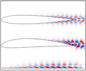
Figures 4 and 5 show the first SPOD mode of the velocity and pressure fields at  $St = 7$ for the NACA 0012 and NACA 4412 airfoils, respectively. The real part of the modes is shown; the imaginary part forms a
  $90^{\circ }$ phase shifted pattern, indicating a downstream travelling wave. All the SPOD results here are multiplied by the square root of the eigenvalue,
  $\sqrt {\lambda _1}$, as in Sinha et al. (Reference Sinha, Rodríguez, Brès and Colonius2014), such that these correspond to fluctuation amplitudes in the flow. We can see that all the results shown in figures 4 and 5 exhibit a coherent wave through most of the airfoil, which begins just after the boundary-layer tripping, with increasing amplitude as it gets closer to the trailing edge, and peak amplitudes in the wake. Comparing the two airfoils, the leading SPOD mode of the 4412 profile has larger fluctuation amplitudes in the wake, but both airfoils have leading SPOD modes with nearly the same amplitudes inside the boundary layer considering the region
  $x/c \leq 0.85$, where the tangential velocity fluctuation amplitude reaches
  $|\widehat {u'}| \approx 0.0025$ for both airfoils. This amplitude scaled in wall units corresponds to
  $|\widehat {u'}^{+}| \approx 0.055$, normalised by
  $u_{\tau }$ and
  $\nu$, for the station
  $x/c=0.65$, where the momentum-thickness Reynolds number is approximately
  $690$ and
  $650$ for the NACA 0012 and NACA 4412 airfoils, respectively. Note that the amplitude of the SPOD modes in viscous scaling is very small with respect to dominant turbulent structures, with fluctuation amplitudes of order unity when scaled in inner units. Therefore, these leading SPOD modes show dominant structures of the TKE of spanwise-averaged fluctuations, as shown in figure 3, but these are only a small part of the bulk of turbulence. Such structures are nonetheless expected to play a significant role in trailing-edge noise, as discussed in the introduction.

Figure 4. First SPOD mode at  $St = 7$ for the NACA 0012 airfoil, representing approximately
  $56\,\%$ of the total kinetic energy of spanwise-averaged fluctuations; (a), (b) and (c) show fluctuations of
  $u$,
$u$,  $v$ and
  $p$, respectively: (a)
  $\sqrt {\lambda _1} \cdot \boldsymbol {\varPsi _{u1}}$; (b)
  $\sqrt {\lambda _1} \cdot \boldsymbol {\varPsi _{v1}}$; and (c)
  $\sqrt {\lambda _1} \cdot \boldsymbol {\varPsi _{p1}}$.

Figure 5. First SPOD mode at  $St = 7$ for the NACA 4412 airfoil, representing approximately
  $60\,\%$ of the total kinetic energy of spanwise-averaged fluctuations; (a), (b) and (c) show fluctuations of
  $u$,
$u$,  $v$ and
  $p$, respectively: (a)
  $\sqrt {\lambda _1} \cdot \boldsymbol {\varPsi _{u1}}$; (b)
  $\sqrt {\lambda _1} \cdot \boldsymbol {\varPsi _{v1}}$; and (c)
  $\sqrt {\lambda _1} \cdot \boldsymbol {\varPsi _{p1}}$.
In order to identify such coherent structures in the flow, we show in figures 6(a) and 6(b) sample instantaneous flow realisations of the spanwise-averaged fluctuations of the tangential velocity and pressure, respectively, for the NACA 0012 airfoil database. Results show that the coherent structures found in the first SPOD mode can be more clearly observed in the pressure field, as figure 6(b) displays instantaneous structures that resemble the pressure fluctuations of the leading SPOD mode shown in figure 4(c). For the velocity field, the coherent structures corresponding to the leading SPOD mode can be observed more clearly in positions further from the wall; for instance, the fluctuations in  $y$ positions further from the wall have a more organised wave behaviour, which is close to the result for the leading SPOD mode of figure 4(a). The clearer observation of coherent waves further from the wall is reminiscent of wavepackets in turbulent jets (Tinney & Jordan Reference Tinney and Jordan2008; Cavalieri et al. Reference Cavalieri, Jordan and Lesshafft2019), which have a clearer structure in the near pressure field. The NACA 4412 airfoil has similar behaviour and results have not been shown here for brevity.

Figure 6. Instantaneous flow realisations taken from the NACA 0012 airfoil database. (a) Tangential velocity fluctuations  $u'$ and (b) pressure fluctuations
  $p'$.
$p'$.
Figures 7 and 8 show the second and third SPOD modes of the tangential velocity component at  $St = 7$ for the NACA 0012 and NACA 4412 airfoils, respectively. Such SPOD modes also display coherent hydrodynamic waves. However, as we increase the order of the mode, the amplitudes of the overall wavy structures decrease, as expected, since their contribution to the total TKE decreases significantly. In particular, differently from the first mode, the amplitudes of velocity fluctuations for the second mode are higher in the turbulent boundary-layer region than in the wake. The third SPOD mode has higher amplitudes near the trailing-edge region, but the wavy structures are noisier due to a worse convergence of higher modes.

Figure 7. Second and third SPOD modes of the tangential velocity component at  $St = 7$ for the NACA 0012 airfoil; (a)
  $\sqrt {\lambda _2} \cdot \boldsymbol {\varPsi _{2}}$ and (b)
  $\sqrt {\lambda _3} \cdot \boldsymbol {\varPsi _{3}}$.

Figure 8. Second and third SPOD modes of the tangential velocity component at  $St = 7$ for the NACA 4412 airfoil; (a)
  $\sqrt {\lambda _2} \cdot \boldsymbol {\varPsi _{2}}$ and (b)
  $\sqrt {\lambda _3} \cdot \boldsymbol {\varPsi _{3}}$.
Such coherent hydrodynamic waves appear in the first SPOD mode of the airfoils even though the boundary layer is at an already fully developed turbulent state. The trailing-edge region features a larger adverse pressure gradient in the boundary layer, which is known to enhance boundary-layer instability for laminar flows (Schmid & Henningson Reference Schmid and Henningson2001), and the present results suggest that a similar mechanism may be at work in the turbulent boundary layers near the trailing edge, especially for the cambered NACA 4412 airfoil. Furthermore, the SPOD results for the tangential velocity component in all cases (see figures 4(b) and 5(b)) show near-wall fluctuations with phase opposition to disturbances towards the boundary-layer edge, which is similar to the behaviour of Tollmien–Schlichting waves, although this is a region of turbulent boundary layer. A similar behaviour was found by Sano et al. (Reference Sano, Abreu, Cavalieri and Wolf2019) for the NACA 0012 airfoil and by Kaplan et al. (Reference Kaplan, Jordan, Cavalieri and Brès2021) for a turbulent boundary layer inside a jet nozzle. The present results indicate that such structures are not just an artefact of a particular database.
In order to further highlight the structures in the boundary-layer region, the wake contribution is neglected in SPOD by imposing zero integral weights  $\boldsymbol {W}$ in the wake region, where
  $x/c>1$. This amounts to considering a subdomain
  $\varOmega$ in (3.1) that excludes the wake. We refer to these as boundary-layer-weighted SPOD modes. The results in that case are shown in figures 9(a) and 9(b) for the NACA 0012 and in figures 10(a) and 10(b) for the NACA 4412 airfoil. The SPOD results now emphasise the hydrodynamic waves near the airfoils, inside the boundary layer. Since the wake region typically has a Kelvin–Helmholtz mode which is much more energetic than the ones from the turbulent boundary layer, which has just stable modes, boundary-layer-weighted SPOD modes highlight more clearly structures within the boundary layer; inspection of the figures shows that these are the same global SPOD modes, but convergence-related noise is lower when the wake is discarded. As the wake dynamics is more thoroughly studied in the literature (see for instance Araya, Colonius & Dabiri Reference Araya, Colonius and Dabiri2017), we will thus focus for the remainder of our analysis on the boundary-layer-weighted modes.

Figure 9. First boundary-layer-weighted SPOD mode at  $St = 7$ for the NACA 0012 airfoil, representing approximately
  $40\,\%$ of the kinetic energy of spanwise-averaged fluctuations; (a)
  $\sqrt {\lambda _1} \cdot \boldsymbol {\varPsi _{1}}$ tangential velocity component
  $\hat {u}'$, (b)
  $\sqrt {\lambda _1} \cdot \boldsymbol {\varPsi _{1}}$ wall-normal velocity component
  $\hat {v}'$.

Figure 10. First boundary-layer-weighted SPOD mode at  $St = 7$ for the NACA 4412 airfoil, representing approximately
  $30\,\%$ of the kinetic energy of spanwise-averaged fluctuations; (a)
  $\sqrt {\lambda _1} \cdot \boldsymbol {\varPsi _{1}}$ tangential velocity component
  $\hat {u}'$, (b)
  $\sqrt {\lambda _1} \cdot \boldsymbol {\varPsi _{1}}$ wall-normal velocity component
  $\hat {v}'$.
4.2. Comparison between SPOD and resolvent modes
In this section we will compare the SPOD results obtained in § 4.1 for both airfoils with the most amplified responses from resolvent analysis. To do so, we will make a locally parallel assumption for the resolvent analysis, and compare the first resolvent mode with the first SPOD mode for some specific stations  $x/c$ of the airfoil by taking a ‘slice’ from the boundary-layer-weighted SPOD results obtained for the entire field in figures 9 and 10.
4.2.1. The base flow
The base flow  $\boldsymbol {\bar {u}}(y_n)$ was extracted from the simulations considering a time and spanwise average. Here, the mean profiles are taken in the wall-normal direction, in the overall
  $x$–
$x$– $y$ coordinate system. For the NACA 0012 airfoil we analysed three different stations:
  $x/c=0.6$,
  $0.7$ and
  $0.9$. For the NACA 4412 airfoil we also analysed three different stations:
  $x/c=0.6$ and
  $0.9$ for the suction side (a) and
  $0.5$ on the pressure side (b), since this airfoil has no symmetry with respect to
  $y=0$. These choices allow consideration of boundary-layer profiles with various degrees of adverse pressure gradient, which is stronger close to the trailing edge, particularly for the NACA 4412 profile, and close to zero for the pressure side of the same airfoil. For all stations considered here, in both airfoils, the boundary-layer profiles are turbulent. Figure 11 shows the mean streamwise velocity around the airfoils, with various
  $x/c$ stations marked by the dashed red lines. The mean velocity profiles at these
  $x/c$ positions for both airfoils are shown in figure 12, scaled in outer units (wing chord
  $c$ and free-stream velocity
  $U_{\infty }$). Figure 13 shows the mean velocity profiles for the same stations in inner units, denoted with a
  $+$ superscript; quantities are made non-dimensional using the friction velocity
  $u_\tau$ and the kinematic viscosity
  $\nu$. The mean velocity profiles in figure 13 show the expected shape of wall-bounded turbulent flows when plotted in inner scale as a function of wall distance
  $y^{+}$. Adverse pressure gradients lead to departures of the typical zero-pressure-gradient profiles, as evident for the NACA 4412 results (see also Vinuesa et al. Reference Vinuesa, Bobke, Örlü and Schlatter2016).

Figure 11. Mean streamwise velocity around the airfoils, with  $x/c=0.4$,
  $0.5$,
  $0.6$,
  $0.7$,
  $0.8$ and
  $0.9$ stations marked by the dashed red lines. (a) NACA 0012 and (b) NACA 4412.

Figure 12. Mean velocity profiles at different positions  $x/c$ for (a) NACA 0012 and NACA 4412 on (b) suction and (c) pressure sides, scaled in outer units.

Figure 13. Mean velocity profiles at different positions  $x/c$ for (a) NACA 0012 and NACA 4412 on (b) suction and (c) pressure sides, scaled in inner units. In all panels, the blue dashed line represents the linear law,
  $\bar {u}^{+} = y^{+}$, and the red dashed line is the log law,
  $\bar {u}^{+} = (1/\kappa ) \ln (y^{+}) + B$, where
  $\kappa = 0.41$ and
  $B=5.2$.
4.2.2. Resolvent parameters
Resolvent analysis was performed for  $St=7$ for comparison with the SPOD results of § 4.1. The streamwise wavenumber
  $k_x$ is also a parameter of resolvent analysis, and is not known a priori, since different wavelengths may appear in the forcing. To study the effect of
  $k_x$ in the resolvent analysis, we first varied
  $k_x$ and studied the leading gains for the three analysed stations of each airfoil. These results are shown in figure 14 for the respective stations analysed in the NACA 0012 airfoil, and in figure 15 for the NACA 4412.

Figure 14. First three resolvent gains as a function of the streamwise wavenumber at  $St = 7$ for the NACA 0012 airfoil; (a)
  $x/c=0.6$, (b)
  $x/c=0.7$ and (c)
  $x/c=0.9$.

Figure 15. First three resolvent gains as a function of the streamwise wavenumber at  $St = 7$ for the NACA 4412 airfoil; (a)
  $x/c=0.5$, (b)
  $x/c=0.6$ and (c)
  $x/c=0.9$.
We notice a sharp peak in all results, which corresponds to disturbances outside the boundary layer, where the phase velocity is equal to the free-stream velocity. Analysis of forcing and response modes for these wavenumbers shows that they correspond to free-stream modes, similar to the observations of Dergham, Sipp & Robinet (Reference Dergham, Sipp and Robinet2013) for a backward-facing step. We have verified that forcing and response modes in these cases have spatial support mostly outside the boundary layer. Such free-stream modes were studied by Nogueira et al. (Reference Nogueira, Cavalieri, Hanifi and Henningson2020) and are not of immediate interest for the boundary-layer dynamics. Besides the sharp peak, we can also notice smooth peaks in all stations for the first gain  $\sigma _{1}$. These peaks correspond to disturbances inside the boundary layer, where the phase velocity is lower than the free-stream velocity. Moreover, for the smooth peaks there is a clear dominance of the optimal forcing, which leads to a response with a gain that is at least one order of magnitude higher than the suboptimals. To perform the resolvent analysis we thus used the
  $k_x$ corresponding to the larger smooth peaks in each analysed section for both airfoils. For the NACA 0012 airfoil we notice that the value used in resolvent analysis,
  $k_x = 50$, corresponds to a wavelength
  $\lambda _x = 0.12$, which closely matches the wavelength of the first SPOD mode shown in figure 4.
4.2.3. Comparison between SPOD and resolvent modes
Results of the comparison between first boundary-layer-weighted SPOD mode and optimal response from resolvent analysis are shown in figures 16 and 17 for the NACA 0012 airfoil for horizontal and vertical velocity components, respectively; and in figures 18 and 19 for the NACA 4412 airfoil, also for horizontal and vertical velocity components, respectively. As commented before, the boundary-layer-weighted SPOD modes were taken to minimise statistical noise.

Figure 16. First SPOD mode (red dashed line) compared with the optimal response from resolvent analysis (black solid line) of the streamwise velocity component  $u$, for the NACA 0012 airfoil, at stations
  $x/c=0.6$,
  $0.7$ and
  $0.9$; (a)
  $\mu \approx 0.80$, (b)
  $\mu \approx 0.83$ and (c)
  $\mu \approx 0.85$.

Figure 17. First SPOD mode (red dashed line) compared with the optimal response from resolvent analysis (black solid line) of the wall-normal velocity component  $v$, for the NACA 0012 airfoil, at stations
  $x/c=0.6$,
  $0.7$ and
  $0.9$; (a)
  $\mu \approx 0.80$, (b)
  $\mu \approx 0.83$ and (c)
  $\mu \approx 0.85$.

Figure 18. First SPOD mode (red dashed line) compared with the optimal response from resolvent analysis (black solid line) of the streamwise velocity component  $u$, for the NACA 4412 airfoil, at stations
  $x/c=0.5$ in the pressure side,
  $x/c=0.6$ and
  $0.9$ in the suction side; (a)
  $\mu \approx 0.75$, (b)
  $\mu \approx 0.67$ and (c)
  $\mu \approx 0.70$.

Figure 19. First SPOD mode (red dashed line) compared with the optimal response from resolvent analysis (black solid line) of the wall-normal velocity component  $v$, for the NACA 4412 airfoil, at stations
  $x/c=0.5$ in the pressure side,
  $x/c=0.6$ and
  $0.9$ in the suction side; (a)
  $\mu \approx 0.75$, (b)
  $\mu \approx 0.67$ and (c)
  $\mu \approx 0.70$.
The comparisons show that the resolvent modes have overall features that correspond to the leading SPOD modes from the databases. In order to perform a quantitative comparison between the first SPOD mode and the optimal response from resolvent analysis, we quantified the agreement between the SPOD eigenfunction  $\varPsi _{1}$ and optimal response from the resolvent analysis
  $U_1$ using the normalised projection given by (3.5), as in Abreu et al. (Reference Abreu, Cavalieri, Schlatter, Vinuesa and Henningson2020a,Reference Abreu, Cavalieri, Schlatter, Vinuesa and Henningsonb). Values of
  $\mu$ close to 1 are indicative of agreement of both amplitudes and phases for both velocity components. The agreement between resolvent and SPOD is closer for the 0012 airfoil, with normalised projections higher than
  $0.8$ for all stations. The comparison for the 4412 airfoil has the best agreement at the pressure side, with a normalised projection of
  $\mu =0.75$. The suction side has agreement metrics close to
  $0.7$. These results can be explained by the fact that the locally parallel resolvent analysis is based on properties in the near wall, which are simpler in the lower adverse pressure gradient from the NACA 0012 than in the complex adverse pressure gradient of the NACA 4412 (interaction of a wider range of scales with stronger adverse pressure gradients), which leads to a stronger inhomogeneity in
  $x$, such that the accuracy of the locally parallel assumption becomes questionable. However, the general features of the SPOD mode are captured by the optimal response for all cases presented in figures 16–19. The double peak structure of the streamwise velocity is related to a phase jump in
  $y$, which may be observed in figure 4(a). Such phase jump is also obtained in the leading resolvent mode, as exemplified in figure 20, which shows phase comparisons for a station of the NACA 0012 airfoil. Other stations show similar results and are not shown here for brevity.

Figure 20. Phase of the first SPOD mode (red dashed line) compared with the phase of the optimal response from resolvent analysis (black solid line) for the streamwise (a) and wall-normal velocity components (b), at the station  $x/c=0.7$ of the NACA 0012 airfoil. (a) Phase of
  $u$ (rad) and (b) Phase of
  $v$ (rad).
Since we deal with a turbulent boundary layer, an exact match is not expected, but the comparisons presented here show that resolvent analysis provides a good reduced-order model for the spanwise-coherent disturbances considered here, which play an important role in the radiation of trailing-edge noise (Sano et al. Reference Sano, Abreu, Cavalieri and Wolf2019). There is close agreement with streamwise velocity fluctuations of the leading SPOD mode, which has an amplitude distribution similar to that of Tollmien–Schlichting waves, with a phase jump at a position with vanishing amplitude, also visible in the SPOD fields in figures 4–10. The relatively low amplitude of the two-dimensional disturbances within the boundary layer tends to ease the application of linearised models.
Resolvent analysis also shows consistent trends when the two airfoils are compared. The comparison of figures 14 and 15 shows that resolvent gains are larger for boundary-layer stations with adverse pressure gradient. This is observed in the SPOD modes of figures 4–10, which display larger amplitudes at the suction side of the NACA 4412 airfoil, particularly close to the trailing edge. The NACA 0012 airfoil fluctuation amplitudes are less significant, and the lowest levels are seen at the pressure side of the NACA 4412 profile. These trends are also observed in the resolvent gains.
5. Domain-size effect on coherent hydrodynamic waves
We have found coherent structures on the airfoil surfaces using SPOD, which were modelled using resolvent analysis. However, the use of spanwise-periodic boundary conditions may be a concern, as it may lead to artificially coherent structures. For instance, in earlier works, computational boxes with short streamwise lengths led to artificially streamwise-coherent structures that remained straight throughout the domain, and the use of larger boxes creates a meandering behaviour (Komminaho, Lundbladh & Johansson Reference Komminaho, Lundbladh and Johansson1996). We here investigate this issue using simulations of the flow over a flat plate, forming a ZPG TBL, with computational domains of different spanwise lengths.
5.1. Turbulence statistics and spectral analysis
Using standard Reynolds decomposition  $u=\bar {u} + u'$, the mean horizontal velocity profiles
  $\bar {u}^{+}$ and the variance profiles of the horizontal velocity fluctuations
  $(\overline { u'}^{+})^{2}$ in inner scaling are shown in figures 21(a) and 21(b), respectively, for the position with
  $Re_{\theta }=990$, which corresponds to approximately the station
  $x/c \approx 0.80$ of the NACA 0012 airfoil and
  $x/c \approx 0.75$ of the NACA 4412 profile. The mean velocity profiles for all the three simulations collapse as expected, and show the typical shape of wall-bounded turbulent flows when plotted as a function of wall distance
  $y^{+}$, following linear and log laws. Variance profiles also collapse for the three simulations, and have the expected pattern characteristic of wall-bounded turbulent flows, with a near-wall peak in the buffer layer at
  $y^{+} \approx 15$ (Eitel-Amor et al. Reference Eitel-Amor, Örlü and Schlatter2014). Note that, despite the moderate resolution of the ZPG TBL simulation, the results presented below do not depend on this choice of lower resolution, which was due to the computational efficiency. In order to verify this statement, results for a finer LES for the smallest spatial domain are shown in Appendix.

Figure 21. (a) The mean flow and (b) horizontal velocity fluctuations at  $Re_{\theta }=990$, scaled in inner units. In both panels, the blue dashed line represents the linear law,
  $\bar {u}^{+} = y^{+}$; and the red dashed line is the log law,
  $\bar {u}^{+} = (1/\kappa ) \ln (y^{+}) + B$, where
  $\kappa = 0.41$ and
  $B=5.2$.
The inner-scaled premultiplied power-spectral density of horizontal velocity fluctuations  $k_{z}^{+} E_{uu}^{+}$ as a function of spanwise wavelength
  $\lambda _z^{+}=2{\rm \pi} / k_z^{+}$ is shown in figure 22(a) at position
  $Re_{\theta }=990$, for all the three simulations. Similarly to the mean profile and the variance, the premultiplied spectra for the three simulations collapse, showing further indication of independence of domain size. Results in figure 22(a) show a peak in the spanwise wavelength corresponding to
  $\lambda _{z}^{+} \approx 100$, which is representative of the signature of the near-wall cycle of streaks and quasi-streamwise vortices. This has been documented in many studies across a range of Reynolds numbers and flow types (Jiménez Reference Jiménez2013). The same inner-scaled power-spectral density of horizontal velocity fluctuations, without premultiplication
  $E_{uu}^{+}$, is shown in figure 22(b) at the same position,
  $Re_{\theta }=990$, for all the three simulations. Figure 22(c) shows the power-spectral density of figure 22(b) for selected wall-normal positions, highlighting the low-wavenumber behaviour. Results show that the power-spectral density contours do not close when premultiplication is not considered, even with the increasing spanwise length
  $L_z$, indicating that there is non-zero power-spectral density for very low wavenumbers
  $k_z^{+} \to 0$, or, equivalently, very large values of
  $\lambda _z^{+}$. We can see that there are structures with
  $k^{+}_{z}=0$, which correspond to two-dimensional perturbations in the computational domain, corresponding to the structures studied for the airfoils for
  $k^{+}_{z}=0$.

Figure 22. Spanwise power-spectral density of the streamwise velocity fluctuation  $u'$ at location
  $Re_{\theta }=990$ for the three ZPG TBL simulations: (a) with premultiplication
  $k_{z}^{+} E_{uu}^{+}$ and
  $x$-axis as
  $\lambda _{z}^{+}$ shown in log scale; and (b) without premultiplication
  $E_{uu}^{+}$ and
  $k_{z}^{+}$ shown in linear scale; and (c) without premultiplication
  $E_{uu}^{+}$ and
  $k_{z}^{+}$ at specific
  $y^{+}$ positions.
The spectrum converges to a finite value at  $k^{+}_{z}=0$ and there is no evidence in the current results, which already include much wider domains than usual, that the power of
  $k^{+}_{z}=0$ will decay to zero. The wavenumber
  $k^{+}_{z} \to 0$ corresponds to spanwise-coherent velocity fluctuations, which have not been studied in detail in the literature and are the main focus of this study. This limit is thus independent of domain size for the computations shown here. As discussed by Lozano-Durán & Jiménez (Reference Lozano-Durán and Jiménez2014), two-dimensional fluctuations in the simulation, for
  $k_z^{+}=0$, represent disturbances whose spanwise length scale is larger than the size of the computational box; they should be thus understood as fluctuations with
  $\lambda _z \gg \delta$, which are responsible for the low-wavenumber behaviour of power-spectral density shown in figure 22(b).
5.2. SPOD and resolvent results
As discussed previously, in order to compare the results obtained with the ZPG TBL simulations with those from the airfoils, we normalised the parameters using the momentum thickness of reference,  $\theta _0$, corresponding to the one taken at
  $60\,\%$ of the NACA 0012 airfoil chord, where the momentum-thickness Reynolds number is approximately
  $600$. The region of interest in the ZPG TBL was considered to be the one corresponding to the trailing-edge region, i.e. between
  $60\,\%$ and
  $80\,\%$ of the airfoil chord length, where the hydrodynamic waves have larger amplitudes. Moreover, the frequency used to perform the SPOD in the airfoils,
  $St \approx 7$, corresponds to
  $St_{\theta } \approx 0.010$ at
  $60\,\%$ of the NACA 0012 airfoil chord. We will then perform the SPOD in the region of interest of the ZPG TBL databases, by proper selection of a domain of interest
  $\varOmega$, considering
  $St_{\theta _0} = 0.010$.
Similarly to the analysis of the airfoil databases, we have taken a spanwise average of flow fluctuations before performing the SPOD, to focus our analysis on spanwise-coherent structures. SPOD for the three ZPG TBL databases was performed in a fully turbulent region delimited by  $600 \leq Re_{\theta } \leq 990$, which corresponds approximately to the NACA 0012 airfoil stations
  $0.60 \leq x/c \leq 0.80$ (see table 1 for the correspondent NACA 4412 airfoil stations). The focus on the region of interest ensures that only fluctuations in the developed turbulent region are considered, with minimal influence from the upstream tripping. Furthermore, the size of the region ensures that disturbances are able to travel across the entire region within the duration of each time segment used in Welch's method.
Figure 23 shows the SPOD eigenvalues for the three ZPG TBL simulations for  $k_z = 0$, which show nearly no change among the three domain sizes. We thus conclude that the coherent structures in all cases have nearly the same amplitude. Figures 24(a–c) and 25(a–c) show the first SPOD mode for horizontal and vertical velocity components, respectively, for all the three ZPG TBL simulations. We can observe the presence of coherent waves for all the cases, with minimal changes as the spanwise length of the domain is varied. The SPOD results for the ZPG TBL databases in these figures display nearly the same mode shapes and amplitudes for the three considered domain sizes, and the structures are very similar to those around the airfoils, shown in figures 9 and 10. For the ZPG TBL modes, the amplitude of the horizontal velocity fluctuation reaches
  $|\widehat {u'}| \approx 0.0028$, or
  $|\widehat {u'}^{+}| \approx 0.061$ in wall units, normalised by
  $u_{\tau }$ and
  $\nu$ from the beginning of the domain,
  $x/\theta _0=0$, where
  $Re_{\theta }=600$. Note that the amplitudes of the SPOD mode of the ZPG TBL are very close to those from the airfoils, and they also make a small contribution to the overall turbulence, but have a potential effect in sound radiation. The present SPOD results indicate that the coherent hydrodynamic waves found in the present study, corresponding to spanwise-coherent disturbances in turbulent boundary layers, have a physical meaning and are not an artefact from the simulations.

Figure 23. SPOD eigenvalues for the three ZPG TBL simulations.

Figure 24. First SPOD mode of the horizontal velocity fluctuations (a,b) compared with the optimal response from resolvent analysis (c,d) for the three analysed ZPG TBL simulations at  $k_z = 0$; (a)
  $\varPsi _{u1}$
  $L_z = 72 \theta _0$, (b)
  $\varPsi _{u1}$
  $L_z = 144 \theta _0$, (c)
  $\varPsi _{u1}$
  $L_z = 288 \theta _0$ and (d) optimal response.

Figure 25. First SPOD mode of the vertical velocity fluctuations (a,b) compared with the optimal response from resolvent analysis (c,d) for the three analysed ZPG TBL simulations at  $k_z = 0$; (a)
  $\varPsi _{v1}$
  $L_z = 72 \theta _0$, (b)
  $\varPsi _{v1}$
  $L_z = 144 \theta _0$, (c)
  $\varPsi _{v1}$
  $L_z = 288 \theta _0$ and (d) optimal response.
Figures 24(d) and 25(d) show the optimal response from resolvent analysis for horizontal and vertical velocity components, respectively, for  $k_z = 0$. In this case, a global resolvent analysis was carried out, allowing a better quantitative comparison with the SPOD modes, since the streamwise wavenumber
  $k_x$ is no longer specified, and appears naturally in the structure of the optimal flow response. As the mean flows of the three simulations are nearly identical, resolvent analysis was computed using the mean velocity for the smallest computational domain. The frequency used to compute the resolvent analysis here was
  $St_{\theta _0}=0.010$. We observe a very close agreement between the SPOD modes and the optimal response from resolvent analysis, for both velocity components. The observed agreement further confirms that spanwise-coherent structures in turbulent boundary layers can be modelled as the most amplified flow response, obtained using the linearised N–S operator.
We now examine non-zero spanwise wavenumbers in order to evaluate if the spanwise-averaged fluctuations of  $k_z=0$ are representative of disturbances for other low spanwise wavenumbers. Figures 26, 27 and 28 show the first SPOD mode and the optimal response from resolvent analysis of the ZPG TBL simulations for the horizontal, vertical and spanwise velocity components, respectively, for
  $k_z = 2{\rm \pi} /L_z$, with
  $L_z$ taken for the smallest domain size, such that this non-zero wavenumber is obtained for the three simulations. We can observe that these results are very similar to the results for
  $k_z = 0$, also showing a coherent wave with similar features. As these are no longer two-dimensional modes, they display a spanwise velocity component, which also has a wave structure. All three velocity components are similarly matched by the leading resolvent mode, which confirms the pertinence of resolvent analysis to model such structures. The observed similarity of
  $u$ and
  $v$ fluctuations of non-zero
  $k_z$ to the
  $k_z=0$ counterparts strongly suggests that two-dimensional fluctuations in the simulations are not spurious modes, and are actually representative of a range of low wavenumbers, or, alternatively, of disturbances with large spanwise coherence.

Figure 26. First SPOD mode of the horizontal velocity fluctuations (a,b) compared with the optimal response from resolvent analysis (c,d) for the three analysed ZPG TBL simulations at  $k_z = 2{\rm \pi} /L_z$; (a)
  $\varPsi _{u1}$
  $L_z = 72 \theta _0$, (b)
  $\varPsi _{u1}$
  $L_z = 144 \theta _0$, (c)
  $\varPsi _{u1}$
  $L_z = 288 \theta _0$ and (d) optimal response.

Figure 27. First SPOD mode of the vertical velocity fluctuations (a,b) compared with the optimal response from resolvent analysis (c,d) for the three analysed ZPG TBL simulations at  $k_z = 2{\rm \pi} /L_z$; (a)
  $\varPsi _{v1}$
  $L_z = 72 \theta _0$, (b)
  $\varPsi _{v1}$
  $L_z = 144 \theta _0$, (c)
  $\varPsi _{v1}$
  $L_z = 288 \theta _0$ and (d) optimal response.

Figure 28. First SPOD mode of the spanwise velocity fluctuations (a,b) compared with the optimal response from resolvent analysis (c,d) for the three analysed ZPG TBL simulations at  $k_z = 2{\rm \pi} /L_z$; (a)
  $\varPsi _{w1}$
  $L_z = 72 \theta _0$, (b)
  $\varPsi _{w1}$
  $L_z = 144 \theta _0$, (c)
  $\varPsi _{w1}$
  $L_z = 288 \theta _0$ and (d) optimal response.
Figures 29(a) and 29(c) show the corresponding forcing from the optimal response presented in figures 24(d) and 25(d), considering  $k_z = 0$, for the horizontal and vertical velocity components, respectively. Figures 29(b), 29(d) and 29(e) show the corresponding forcing from the optimal response presented in figures 26(d) and 27(d), considering
  $k_z = 2{\rm \pi} /L_z$, for the horizontal, vertical and spanwise velocity components, respectively. Notice that, whereas the domain of interest for the flow response was taken in the downstream region of the computational domain, corresponding to the region analysed using SPOD, the optimal forcing was determined throughout the physical domain, as it is known that the optimal forcing typically appears upstream of the flow response. The forcing modes also display a wave structure, with fluctuations inclined against the shear, which suggests that the forcing exploits the Orr mechanism, similar to the optimal excitation of Tollmien–Schlichting waves (Åkervik et al. Reference Åkervik, Ehrenstein, Gallaire and Henningson2008), and to coherent boundary-layer disturbances inside a nozzle (Garnaud et al. Reference Garnaud, Lesshafft, Schmid and Huerre2013; Kaplan et al. Reference Kaplan, Jordan, Cavalieri and Brès2021).

Figure 29. Optimal forcing from the resolvent analysis for the ZPG TBL simulations; (a)  $f_x$ for
  $k_z = 0$, (b)
  $f_x$ for
  $k_z = 2{\rm \pi} /L_z$, (c)
  $f_y$ for
  $k_z = 0$, (d)
  $f_y$ for
  $k_z = 2{\rm \pi} /L_z$ and (e)
  $f_z$ for
  $k_z = 2{\rm \pi} /L_z$.
6. Conclusions
In the current work we have used SPOD to extract the most energetic spanwise-coherent structures from the turbulent flow around two different airfoils: NACA 0012 with zero angle of attack and NACA 4412 with an angle of attack  $AoA=5^{\circ }$, both for chord Reynolds number
  $Re_c = 400\,000$. We found in the leading SPOD mode of spanwise-averaged fluctuations, which is statistically converged in our database, a coherent wave that propagates all the way from the transition region to the trailing edge. The study by Sano et al. (Reference Sano, Abreu, Cavalieri and Wolf2019), shows that such structures are a dominant non-compact source in trailing-edge noise. Thus, although these spanwise-coherent structures are not much studied in the literature of wall-bounded turbulence, they are relevant for aeroacoustics (Amiet Reference Amiet1976; Nogueira et al. Reference Nogueira, Cavalieri and Jordan2017).
The observed hydrodynamic waves in the leading SPOD modes were modelled using locally parallel resolvent analysis, where turbulent mean profiles from specific stations  $x/c$ in both airfoils were used as base flows. Results of comparisons for all the cases presented here for both airfoils show a fair agreement between the optimal flow response and the leading SPOD mode. Moreover, the optimal response has a gain which is at least an order of magnitude larger than the suboptimals, which explains its presence in the data series for the turbulent boundary layers. The results indicate that resolvent analysis is a pertinent reduced-order model for the relevant fluctuations, leading to predictions of the structure of advecting waves reaching the edge.
In order to show the domain-size independence and ensure the physical relevance of such structures found around the airfoils, we run three simulations of a ZPG TBL for three different spanwise domain lengths:  $L_z=72 \theta _0$,
  $L_z=144 \theta _0$ and
  $L_z=288 \theta _0$, where
  $\theta _0$ is a reference momentum thickness, taken towards the end of the computational domain. A spectral analysis of the flow, considering a power-spectral density of the horizontal velocity fluctuations without the usual premultiplication adopted in wall turbulence, showed the presence of spanwise-coherent structures with
  $k_{z}^{+} \to 0$, which have no signature in standard premultiplied spectra. SPOD results also showed the presence of such hydrodynamic waves for all three computational domains, with nearly the same amplitude. Thus, our results indicate that these coherent hydrodynamic waves have physical meaning and are not just an artefact from the simulation. They should be understood as spanwise-coherent disturbances, the characteristic length of which is much larger than the boundary-layer thickness. Such disturbances appear as two-dimensional disturbances in the considered numerical simulations with periodic boundary conditions in
  $z$. Coherent structures in the ZPG TBL were modelled with global resolvent analysis, and the leading resolvent mode closely matches the first SPOD mode of the simulations. Consideration of low, but non-zero, spanwise wavenumbers also leads to similar wavy disturbances in the first SPOD mode, which are accurately modelled using resolvent analysis.
In summary, the present work reveals that, among the dominant features in the turbulent boundary layers around the airfoil, such as streaky structures with the usual spanwise spacing of 100 viscous units, there are also well-defined spanwise-coherent hydrodynamic waves, with peak at  $St \approx 7$, i.e. the same frequency found to be correlated to the acoustic radiation in Sano et al. (Reference Sano, Abreu, Cavalieri and Wolf2019). The structures studied in this work are not the standard streaky structures of turbulent boundary layers; these are instead low-energy, coherent spanwise-elongated waves reminiscent of those identified by Hussain & Reynolds (Reference Hussain and Reynolds1972) in their early work on forced oscillations in turbulent channel flow. In this paper we have shown the presence of such structures in various wall-bounded turbulent flows, and these are appropriately modelled as the optimal flow response from resolvent analysis. Further numerical and experimental work aiming at the characterisation of such structures is promising.
Funding
The authors acknowledge the financial support received from Conselho Nacional de Desenvolvimento Científico e Tecnológico, CNPq, under grant No. 310523/2017-6, and by CAPES through the PROEX program. Financial support provided by the Knut and Alice Wallenberg Foundation is also gratefully acknowledged. We also acknowledge funding from Centro de Pesquisa e Inovação Sueco-Brasileiro (CISB) and from the Swedish Research Council through grant agreement no. 2018-05973. The simulations were performed on resources provided by the Swedish National Infrastructure for Computing (SNIC) at the PDC Center for High Performance Computing at KTH, Stockholm.
Declaration of interests
The author reports no conflict of interest.
Appendix
In order to evaluate the dependence of the results on the LES resolution, we analysed a finer LES of the ZPG TBL. Figures 30(a) and 30(b) show the mean horizontal velocity profiles  $\bar {u}^{+}$ and the variance profiles of the horizontal velocity fluctuations
  $(\overline { u'}^{+})^{2}$ in inner scaling, respectively, for the position with
  $Re_{\theta }=990$. The mean velocity profile shows the expected shape of a turbulent boundary layer, which matches the results from Schlatter & Örlü (Reference Schlatter and Örlü2012). The variance profile has the expected pattern characteristic of wall-bounded turbulent flows. The SPOD modes for the ZPG TBL database considering a finer mesh is shown in figure 31. We can notice that the SPOD results are nearly the same as those from § 5.2.

Figure 30. (a) The mean flow and (b) horizontal velocity fluctuations at  $Re_{\theta }=990$, scaled in inner units, compared with results of ZPG TBL from Schlatter & Örlü (Reference Schlatter and Örlü2012) for
  $Re_{\theta }=1000$. In both panels, the blue dashed line represents the linear law,
  $\bar {u}^{+} = y^{+}$; and the red dashed line is the log law,
  $\bar {u}^{+} = (1/\kappa ) \ln (y^{+}) + B$, where
  $\kappa = 0.41$ and
  $B=5.2$.

Figure 31. First SPOD mode of the horizontal (a,b) and vertical velocity fluctuations (c,d) of the finer LES of the ZPG TBL at  $k_z = 0$ (a,c) and
  $k_z = 2{\rm \pi} /L_z$ (c,d); (a)
  $\varPsi _{u1}$
  $k_z = 0$, (b)
  $\varPsi _{u1}$
  $k_z = 2{\rm \pi} /L_z$, (c)
  $\varPsi _{v1}$
  $k_z = 0$ and (d)
  $\varPsi _{v1}$
  $k_z = 2{\rm \pi} /L_z$.


