


1 Introduction
Pressure fluctuations from high-speed flows pose serious risks and design challenges in many engineering applications. For example, there is a need to reduce the sound intensity near aircraft during take-off and landing to protect personnel (Kaltenbach, Maschke & Klinke Reference Kaltenbach, Maschke and Klinke2008). In addition, regulations are placed to reduce environmental noise pollution from commercial aircraft near cities, described in Bowes et al. (Reference Bowes, Rumpf, Bowler, Carnes, Fratarangelo, Heiser, Hu, Moin and Voorhees2009). Launch pad configurations for rockets address some of these issues by using water injection systems to reduce pressure fluctuations and thermal loading (Himelblau et al.
Reference Himelblau, Kern, Manning, Piersol and Rubin2001; Ignatius, Sathiyavageeswaran & Chakravarthy Reference Ignatius, Sathiyavageeswaran and Chakravarthy2014). In such configurations, sound reduction depends on the injection geometry, injection flow rate and mass flux ratio (Zoppellari & Juve Reference Zoppellari and Juve1997; Krothapalli et al.
Reference Krothapalli, Venkatakrishnan, Lourenco, Greska and Elavarasan2003; Norum Reference Norum2004), in addition to jet temperature (Norum Reference Norum2004; Henderson Reference Henderson2010). Microjet injection of water into high-speed jet turbulence has been observed to reduce far-field sound levels by 2–6 dB using 5 %–17 % of the mass of the gas jet (Krothapalli et al.
Reference Krothapalli, Venkatakrishnan, Lourenco, Greska and Elavarasan2003). At even larger mass loadings (
 ${>}100\,\%$
of jet mass), a 12 dB reduction of the sound near rocket engine exhausts was achieved (Zoppellari & Juve Reference Zoppellari and Juve1997). However, in similar jet configurations, sound radiation has been observed to increase due to fluid injection, suggesting its control and mechanisms toward noise reduction are not universal (e.g. Gilinsky, Bhat & Seiner Reference Gilinsky, Bhat and Seiner1994, and references therein).
${>}100\,\%$
of jet mass), a 12 dB reduction of the sound near rocket engine exhausts was achieved (Zoppellari & Juve Reference Zoppellari and Juve1997). However, in similar jet configurations, sound radiation has been observed to increase due to fluid injection, suggesting its control and mechanisms toward noise reduction are not universal (e.g. Gilinsky, Bhat & Seiner Reference Gilinsky, Bhat and Seiner1994, and references therein).
Velocity fluctuations in high-speed shear-flow turbulence provide sources of radiated pressure fluctuations (Lighthill Reference Lighthill1952). For supersonic jets injected with water azimuthally near the jet exit, particle image velocimetry (PIV) data show a reduction in turbulence intensity without a sizable change to the mean flow profile (Krothapalli et al. Reference Krothapalli, Venkatakrishnan, Lourenco, Greska and Elavarasan2003), which has implications for the radiated sound. Turbulence correlation length scales also decrease from water droplet-injected shear layers (Krothapalli et al. Reference Krothapalli, Venkatakrishnan, Lourenco, Greska and Elavarasan2003). In addition, micro-jet injection leads to a streamwise oriented vorticity pattern. Without fluid injection, similar vorticity structures have been observed through geometric modifications to the jet nozzles. By adding chevrons (Alkislar & Butler Reference Alkislar and Butler2007) or likewise using contoured nozzle inserts (e.g. Murray & Lyons Reference Murray and Lyons2016), aimed to augment near-nozzle shear layer development, these strategies also achieve a sound reduction, which suggests a shared reduction mechanism with water injection via changes to the turbulence. In isolation, the sensitivity of sound radiation to reduced turbulence correlation, intensity and relative convection velocity are known to a degree (Lighthill Reference Lighthill1952; Ffowcs Williams Reference Ffowcs Williams1963). However, the mechanisms of how a disperse phase (e.g. droplets or particles) couple to the turbulence and pressure field are not fully understood, which limits advancements toward controlling such flows.
Since inertial particles are known to modify incompressible turbulence (see e.g. Balachandar & Eaton Reference Balachandar and Eaton2010, and references therein), these effects, when translated into a compressible regime, are expected to change the pressure fluctuations and sound field radiation. Drag induced by individual particles in turbulent flows can enhance or suppress velocity-fluctuation amplitudes over a wide range of scales, which depend on, for example, the particle size relative to the Kolmogorov length scale, the mean velocity difference between the phases and the particle-to-fluid mass ratio (Elghobashi & Truesdell Reference Elghobashi and Truesdell1993; Balachandar & Eaton Reference Balachandar and Eaton2010; Capecelatro, Desjardins & Fox Reference Capecelatro, Desjardins and Fox2015, Reference Capecelatro, Desjardins and Fox2018). In the dilute limit, gas-phase turbulence accumulates particles in high-strain regions of the flow (Eaton & Fessler Reference Eaton and Fessler1994; Rouson & Eaton Reference Rouson and Eaton2001; Marchioli & Soldati Reference Marchioli and Soldati2002; Balachandar & Eaton Reference Balachandar and Eaton2010), and at higher particle loading it can give rise to the spontaneous generation of densely packed particle regions (Glasser, Sundaresan & Kevrekidis Reference Glasser, Sundaresan and Kevrekidis1998; Noymer & Glicksman Reference Noymer and Glicksman2000; Agrawal et al.
Reference Agrawal, Loezos, Syamlal and Sundaresan2001; Capecelatro et al.
Reference Capecelatro, Desjardins and Fox2015), i.e. clusters, which have been observed to hinder mixing between the phases (Agrawal et al.
Reference Agrawal, Holloway, Milioli, Milioli and Sundaresan2013; Shaffer et al.
Reference Shaffer, Gopalan, Breault, Cocco, Karri, Hays and Knowlton2013) and amplify the aforementioned two-way-coupled effects. Recent data show that large-scale velocity gradients affect the turbulent transport of small (Kolmogorov-scale) heavy particles and the clustering process at small scales (Nicolai, Jacob & Piva Reference Nicolai, Jacob and Piva2013). Gualtieri, Picano & Casciola (Reference Gualtieri, Picano and Casciola2009) demonstrated that large-scale shear generates anisotropic velocity fluctuations which, in turn, arrange particle configurations in directionally biased clusters. In temporally developing shear layers, the mixing layer growth rate and turbulent kinetic energy (TKE) were observed to reduce with mass loading; however, these changes were insensitive to the Stokes numbers considered (Miller & Bellan Reference Miller and Bellan1999; Okong’o & Bellan Reference Okong’o and Bellan2004; Leboissetier, Okong’o & Bellan Reference Leboissetier, Okong’o and Bellan2005). Similarly, for homogeneous shear turbulence, Battista et al. (Reference Battista, Gualtieri, Mollicone and Casciola2018) recently demonstrated that particles with Stokes number
 $St_{\unicode[STIX]{x1D702}}=O(1)$
, based on the Kolmogorov scale, suppress TKE across the entire range of resolved scales as the mass loading is increased.
$St_{\unicode[STIX]{x1D702}}=O(1)$
, based on the Kolmogorov scale, suppress TKE across the entire range of resolved scales as the mass loading is increased.
Using the foundational aeroacoustics theory of Lighthill (Reference Lighthill1952), Crighton & Ffowcs Williams (Reference Crighton and Ffowcs Williams1969) showed that a disperse phase (such as air bubbles or dust particles) flowing in turbulence has additional sources of sound via volume fraction and interphase force mechanisms. Atop the sound from the turbulence, these additional sound sources are anticipated to be substantial, with an up to 20 dB increase in sound pressure levels (Crighton & Ffowcs Williams Reference Crighton and Ffowcs Williams1969). Contrary to these theoretical estimates, micro-droplet water injection into the high-speed-jet shear layers reduce sound intensity (Krothapalli et al. Reference Krothapalli, Venkatakrishnan, Lourenco, Greska and Elavarasan2003), suggesting, in part, unknown sound reduction mechanisms. This contradiction has consequence and begs the question: are observed sound reductions near high-speed jets, injected with water droplets, formed from a mixture of sound reduction mechanisms that outpace theoretically large sound sources from the disperse phase itself? The answer has implications for sound-reduction strategies applied to single-phase turbulence, which inherently lack potentially loud sound sources due to particles. As will be shown, results indicate an important Mach number and mass loading dependence for sound and turbulence changes, which suggests extensions to theoretical expectations for regimes considered here. These concepts will be revisited in § 4.
Eulerian–Lagrangian simulations of particle-laden free-shear-flow turbulence are used to provide the space–time dynamics leading to changes in the near-field pressure fluctuations compared to unladen turbulence. In the following section, starting from a mesoscale description for compressible two-phase flows, a transport equation for the gas-phase pressure intensity in the presence of particles is derived. The free-shear-flow turbulence configurations and numerical methods are discussed in § 3. Analysis of turbulence statistics for the parametric study based on Mach number (
 $M$
), mass loading (
$M$
), mass loading (
 $\unicode[STIX]{x1D6F7}_{m}$
) and Stokes number (
$\unicode[STIX]{x1D6F7}_{m}$
) and Stokes number (
 $St$
) are provided in § 4. This is followed by an analysis of the mechanisms of local pressure intensity changes in the turbulence using the transport budget derived in § 2. The effect of particles on the near-field pressure characteristics are then provided. Finally, the results are summarized in § 5.
$St$
) are provided in § 4. This is followed by an analysis of the mechanisms of local pressure intensity changes in the turbulence using the transport budget derived in § 2. The effect of particles on the near-field pressure characteristics are then provided. Finally, the results are summarized in § 5.
2 Pressure intensity transport in the presence of particles
In this study, mechanisms of pressure intensity changes are examined via a detailed analysis of a transport budget, which necessitates deriving a consistent Reynolds-averaged pressure intensity equation. Unlike in single-phase flows where the Navier–Stokes equations can be directly averaged to obtain a macroscopic description (i.e. a model for the mean flow), special care needs to be taken for turbulent multiphase flows. As discussed in Fox (Reference Fox2014), averaging the microscale equations (a model that solves the Navier–Stokes equation for the fluid with appropriate boundary conditions at the two-phase interface), omits important interphase coupling terms (e.g. Capecelatro et al. Reference Capecelatro, Desjardins and Fox2015). As such, deriving the averaged equations starting from a mesoscale description retains physics by explicitly accounting for volume fraction and interphase coupling terms. In this section, the volume-filtered compressible flow equations are presented and are used to derive the pressure intensity transport that explicitly include multiphase effects.
2.1 A mesoscale description for compressible two-phase flows
To arrive at a mesoscale description for compressible particle-laden flows, the Navier–Stokes equations are split into microscale processes that take place on the scale of a particle and below, and meso- to macroscale processes that take place on a scale much larger than the particle size. Anderson & Jackson (Reference Anderson and Jackson1967) provide such a basis for this approach by applying a local volume filtering operator to the incompressible Navier–Stokes equations, thereby replacing the point variables (fluid velocity, pressure, etc.) by filtered fields. Applying a similar approach to the viscous compressible Navier–Stokes equations, the volume-filtered conservation equations can be expressed as (see appendix A for details)
 $$\begin{eqnarray}\displaystyle & \displaystyle \frac{\unicode[STIX]{x2202}\unicode[STIX]{x1D6FC}\unicode[STIX]{x1D70C}}{\unicode[STIX]{x2202}t}+\unicode[STIX]{x1D735}\boldsymbol{\cdot }(\unicode[STIX]{x1D6FC}\unicode[STIX]{x1D70C}\boldsymbol{u})=0, & \displaystyle\end{eqnarray}$$
 $$\begin{eqnarray}\displaystyle & \displaystyle \frac{\unicode[STIX]{x2202}\unicode[STIX]{x1D6FC}\unicode[STIX]{x1D70C}\boldsymbol{u}}{\unicode[STIX]{x2202}t}+\unicode[STIX]{x1D735}\boldsymbol{\cdot }(\unicode[STIX]{x1D6FC}\{\unicode[STIX]{x1D70C}\boldsymbol{u}\otimes \boldsymbol{u}+p\mathbb{I}-\unicode[STIX]{x1D749}\})=(p\mathbb{I}-\unicode[STIX]{x1D749})\boldsymbol{\cdot }\unicode[STIX]{x1D735}\unicode[STIX]{x1D6FC}+\boldsymbol{F}, & \displaystyle\end{eqnarray}$$
and
 $$\begin{eqnarray}\displaystyle \frac{\unicode[STIX]{x2202}\unicode[STIX]{x1D6FC}\unicode[STIX]{x1D70C}E}{\unicode[STIX]{x2202}t}+\unicode[STIX]{x1D735}\boldsymbol{\cdot }\unicode[STIX]{x1D6FC}(\{\unicode[STIX]{x1D70C}E+p\}\boldsymbol{u}-\boldsymbol{u}\boldsymbol{\cdot }\unicode[STIX]{x1D749})+\unicode[STIX]{x1D6FC}\unicode[STIX]{x1D735}\boldsymbol{\cdot }\boldsymbol{q}=(\unicode[STIX]{x1D749}-p\mathbb{I})\boldsymbol{ : }\unicode[STIX]{x1D735}(\unicode[STIX]{x1D6FC}_{p}\boldsymbol{u}_{p})+\boldsymbol{u}_{p}\boldsymbol{\cdot }\boldsymbol{F}, & & \displaystyle\end{eqnarray}$$
where
 $\unicode[STIX]{x1D6FC}$
is the fluid-phase volume fraction,
$\unicode[STIX]{x1D6FC}$
is the fluid-phase volume fraction,
 $\unicode[STIX]{x1D70C}$
is the fluid density,
$\unicode[STIX]{x1D70C}$
is the fluid density,
 $\boldsymbol{u}$
the fluid velocity,
$\boldsymbol{u}$
the fluid velocity,
 $\boldsymbol{u}_{p}$
is the particle-phase velocity (in an Eulerian frame of reference) and
$\boldsymbol{u}_{p}$
is the particle-phase velocity (in an Eulerian frame of reference) and
 $E$
the total energy. Interphase heat transfer (based on the flow configuration in § 3) had negligible effect on the results and is neglected here. Flow variables in equations (2.1)–(2.3) have been non-dimensionalized by ambient density
$E$
the total energy. Interphase heat transfer (based on the flow configuration in § 3) had negligible effect on the results and is neglected here. Flow variables in equations (2.1)–(2.3) have been non-dimensionalized by ambient density
 $\unicode[STIX]{x1D70C}_{\infty }^{\star }$
, speed of sound
$\unicode[STIX]{x1D70C}_{\infty }^{\star }$
, speed of sound
 $c_{\infty }^{\star }$
, a characteristic length scale
$c_{\infty }^{\star }$
, a characteristic length scale
 $L^{\star }$
(based on vorticity thickness defined in equation (3.3)) and heat capacity at constant pressure
$L^{\star }$
(based on vorticity thickness defined in equation (3.3)) and heat capacity at constant pressure
 $C_{p}^{\star }$
. Dimensional quantities are denoted by a superscript
$C_{p}^{\star }$
. Dimensional quantities are denoted by a superscript
 $\star$
, and the subscript
$\star$
, and the subscript
 $\infty$
indicates reference quantities (taken to be air). The source term
$\infty$
indicates reference quantities (taken to be air). The source term
 $\boldsymbol{F}$
appearing in equations (2.2) and (2.3) accounts for momentum coupling between the particle and gas phases, and its form will be discussed in § 3.2. The non-dimensional viscous stress tensor is given by
$\boldsymbol{F}$
appearing in equations (2.2) and (2.3) accounts for momentum coupling between the particle and gas phases, and its form will be discussed in § 3.2. The non-dimensional viscous stress tensor is given by
 $$\begin{eqnarray}\displaystyle \unicode[STIX]{x1D749}=\frac{\unicode[STIX]{x1D707}}{Re_{c}}(\unicode[STIX]{x1D735}\boldsymbol{u}+\unicode[STIX]{x1D735}\boldsymbol{u}^{\mathsf{T}})+\frac{\unicode[STIX]{x1D706}}{Re_{c}}\unicode[STIX]{x1D735}\boldsymbol{\cdot }\boldsymbol{u} & & \displaystyle\end{eqnarray}$$
and the heat flux
 $\boldsymbol{q}$
is
$\boldsymbol{q}$
is
 $$\begin{eqnarray}\displaystyle \boldsymbol{q}=-\frac{\unicode[STIX]{x1D707}}{Re_{c}Pr}\unicode[STIX]{x1D735}T, & & \displaystyle\end{eqnarray}$$
where
 $Pr\equiv C_{p}^{\star }\unicode[STIX]{x1D707}^{\star }/k^{\star }=0.7$
is the Prandtl number, with
$Pr\equiv C_{p}^{\star }\unicode[STIX]{x1D707}^{\star }/k^{\star }=0.7$
is the Prandtl number, with
 $\unicode[STIX]{x1D707}^{\star }$
and
$\unicode[STIX]{x1D707}^{\star }$
and
 $k^{\star }$
the dynamic viscosity and thermal conductivity, respectively. The Reynolds number used in the formulation is defined as
$k^{\star }$
the dynamic viscosity and thermal conductivity, respectively. The Reynolds number used in the formulation is defined as
 $Re_{c}=Re/M$
, where
$Re_{c}=Re/M$
, where
 $Re=\unicode[STIX]{x1D70C}_{\infty }^{\star }\unicode[STIX]{x0394}U^{\star }L^{\star }/\unicode[STIX]{x1D707}_{\infty }^{\star }$
is the flow Reynolds number with
$Re=\unicode[STIX]{x1D70C}_{\infty }^{\star }\unicode[STIX]{x0394}U^{\star }L^{\star }/\unicode[STIX]{x1D707}_{\infty }^{\star }$
is the flow Reynolds number with
 $\unicode[STIX]{x0394}U^{\star }$
a characteristic velocity defined later, and
$\unicode[STIX]{x0394}U^{\star }$
a characteristic velocity defined later, and
 $M=\unicode[STIX]{x0394}U^{\star }/c_{\infty }^{\star }$
is the Mach number. The non-dimensional viscosity is modelled as a power law
$M=\unicode[STIX]{x0394}U^{\star }/c_{\infty }^{\star }$
is the Mach number. The non-dimensional viscosity is modelled as a power law
 $\unicode[STIX]{x1D707}=[(\unicode[STIX]{x1D6FE}-1)T]^{n}$
, with
$\unicode[STIX]{x1D707}=[(\unicode[STIX]{x1D6FE}-1)T]^{n}$
, with
 $n=0.666$
as a model for air and
$n=0.666$
as a model for air and
 $\unicode[STIX]{x1D6FE}=1.4$
is the ratio of specific heats. The second coefficient of viscosity is given by
$\unicode[STIX]{x1D6FE}=1.4$
is the ratio of specific heats. The second coefficient of viscosity is given by
 $\unicode[STIX]{x1D706}=\unicode[STIX]{x1D707}_{B}-\frac{2}{3}\unicode[STIX]{x1D707}$
, where the bulk viscosity
$\unicode[STIX]{x1D706}=\unicode[STIX]{x1D707}_{B}-\frac{2}{3}\unicode[STIX]{x1D707}$
, where the bulk viscosity
 $\unicode[STIX]{x1D707}_{B}=0.6\unicode[STIX]{x1D707}$
is chosen as a model for the bulk viscosity of air. Assuming an ideal gas, the thermodynamic pressure and temperature depend on
$\unicode[STIX]{x1D707}_{B}=0.6\unicode[STIX]{x1D707}$
is chosen as a model for the bulk viscosity of air. Assuming an ideal gas, the thermodynamic pressure and temperature depend on
 $$\begin{eqnarray}\displaystyle p=(\unicode[STIX]{x1D6FE}-1)(\unicode[STIX]{x1D70C}E-{\textstyle \frac{1}{2}}\unicode[STIX]{x1D70C}\boldsymbol{u}\boldsymbol{\cdot }\boldsymbol{u}) & & \displaystyle\end{eqnarray}$$
and
 $$\begin{eqnarray}\displaystyle T=\frac{\unicode[STIX]{x1D6FE}p}{\unicode[STIX]{x1D70C}(\unicode[STIX]{x1D6FE}-1)}. & & \displaystyle\end{eqnarray}$$
Since pressure is a key observable in the simulations, its transport equation is useful for examining the competition of the mechanisms generating it. Differentiating equation (2.6) with respect to time and substituting equations (2.1)–(2.3) yields the pressure evolution equation in the presence of a disperse phase,
 $$\begin{eqnarray}\displaystyle \frac{\text{D}p}{\text{D}t}=-\unicode[STIX]{x1D6FE}p\unicode[STIX]{x1D735}\boldsymbol{\cdot }\boldsymbol{u}+{\mathcal{D}}-\unicode[STIX]{x1D6FE}p\frac{\text{D}\ln \unicode[STIX]{x1D6FC}}{\text{D}t}+\frac{\unicode[STIX]{x1D6FE}-1}{\unicode[STIX]{x1D6FC}}(\boldsymbol{u}_{p}-\boldsymbol{u})\boldsymbol{\cdot }\boldsymbol{F}, & & \displaystyle\end{eqnarray}$$
where
 $\text{D}/\text{D}t=\unicode[STIX]{x2202}/\unicode[STIX]{x2202}t+\boldsymbol{u}\boldsymbol{\cdot }\unicode[STIX]{x1D735}$
is the material derivative operator and terms involving molecular transport effects are combined into
$\text{D}/\text{D}t=\unicode[STIX]{x2202}/\unicode[STIX]{x2202}t+\boldsymbol{u}\boldsymbol{\cdot }\unicode[STIX]{x1D735}$
is the material derivative operator and terms involving molecular transport effects are combined into
 $$\begin{eqnarray}\displaystyle {\mathcal{D}}=\frac{\unicode[STIX]{x1D6FE}-1}{\unicode[STIX]{x1D6FC}}(\unicode[STIX]{x1D749}\boldsymbol{ : }\unicode[STIX]{x1D735}\unicode[STIX]{x1D6FC}\boldsymbol{u}+\unicode[STIX]{x1D749}\boldsymbol{ : }\unicode[STIX]{x1D735}\unicode[STIX]{x1D6FC}_{p}\boldsymbol{u}_{p})+\unicode[STIX]{x1D6FE}\unicode[STIX]{x1D735}\boldsymbol{\cdot }\frac{\unicode[STIX]{x1D707}}{Re_{c}\,Pr}\unicode[STIX]{x1D735}(p/\unicode[STIX]{x1D70C}). & & \displaystyle\end{eqnarray}$$
Compared to the single-phase pressure transport equation (e.g. Pantano & Sarkar Reference Pantano and Sarkar2002), the last two terms on the right-hand side of equation (2.8) represent new contributions due to the presence of particles. The second-to-last term on the right-hand side involves convection aligned with volume fraction gradients as well as a mechanism associated with the so-called
 $pDV$
work term (Lhuillier, Theofanous & Liou Reference Lhuillier, Theofanous and Liou2010). The last term on the right-hand side represents work due to drag which is only active when the slip velocity magnitude between the phases is
$pDV$
work term (Lhuillier, Theofanous & Liou Reference Lhuillier, Theofanous and Liou2010). The last term on the right-hand side represents work due to drag which is only active when the slip velocity magnitude between the phases is
 $|\boldsymbol{u}_{p}-\boldsymbol{u}|>0$
.
$|\boldsymbol{u}_{p}-\boldsymbol{u}|>0$
.
2.2 Averaged pressure intensity
For examining mechanisms affecting the pressure intensity in turbulence, we use Reynolds decomposition with spatial averaging operator
 $\overline{(\cdot )}$
, such that any quantity
$\overline{(\cdot )}$
, such that any quantity
 $A$
can be decomposed into
$A$
can be decomposed into
 $A=\overline{A}+A^{\prime }$
as is often used to examine Reynolds stress or turbulent kinetic energy transport.
$A=\overline{A}+A^{\prime }$
as is often used to examine Reynolds stress or turbulent kinetic energy transport.
Using this decomposition, multiplying equation (2.8) by
 $p$
and rearranging yields the following pressure intensity transport equation
$p$
and rearranging yields the following pressure intensity transport equation
 $$\begin{eqnarray}\displaystyle & & \displaystyle \frac{\unicode[STIX]{x2202}\overline{p^{\prime }p^{\prime }}}{\unicode[STIX]{x2202}t}+\overline{\boldsymbol{u}}\boldsymbol{\cdot }\unicode[STIX]{x1D735}\overline{(p^{\prime }p^{\prime })}=-2\unicode[STIX]{x1D6FE}\overline{p}~\overline{p^{\prime }\unicode[STIX]{x1D735}\boldsymbol{\cdot }\boldsymbol{u}^{\prime }}-(2\unicode[STIX]{x1D6FE}-1)\overline{p^{\prime }p^{\prime }\unicode[STIX]{x1D735}\boldsymbol{\cdot }\boldsymbol{u}^{\prime }}\nonumber\\ \displaystyle & & \displaystyle \quad -\,2\overline{\boldsymbol{u}^{\prime }p^{\prime }}\boldsymbol{\cdot }\unicode[STIX]{x1D735}\overline{p}-\unicode[STIX]{x1D735}\boldsymbol{\cdot }(\overline{p^{\prime }p^{\prime }\boldsymbol{u}^{\prime }})-2\unicode[STIX]{x1D6FE}\overline{p^{\prime }p^{\prime }}\unicode[STIX]{x1D735}\boldsymbol{\cdot }\overline{\boldsymbol{u}}+\underbrace{2\overline{p^{\prime }{\mathcal{D}}^{\prime }}}_{\hspace{-72.0pt}\text{viscous and heat conduction}}\nonumber\\ \displaystyle & & \displaystyle \quad \times \,\underbrace{-2\unicode[STIX]{x1D6FE}\left(\overline{p^{\prime }p^{\prime }\frac{\text{D}\ln (\unicode[STIX]{x1D6FC})}{\text{D}t}}+\overline{p}~\overline{p^{\prime }\frac{\text{D}\ln (\unicode[STIX]{x1D6FC})}{\text{D}t}}\right)}_{\text{volume}\;\text{displacement}}\nonumber\\ \displaystyle & & \displaystyle +\,\underbrace{2(\unicode[STIX]{x1D6FE}-1)\left(\overline{\frac{p^{\prime }\boldsymbol{F}}{\unicode[STIX]{x1D6FC}}}\boldsymbol{\cdot }(\overline{\boldsymbol{u}_{p}}-\overline{\boldsymbol{u}})+\overline{\frac{p^{\prime }\boldsymbol{F}}{\unicode[STIX]{x1D6FC}}\boldsymbol{\cdot }(\boldsymbol{u}_{p}^{\prime }-\boldsymbol{u}^{\prime })}\right)}_{\text{drag}\;\text{coupling}}.\end{eqnarray}$$
The first two lines of equation (2.10) have the same form as for single-phase flows, and they have been analysed for several turbulence configurations (e.g. Sarkar Reference Sarkar1992). As shown by Sarkar (Reference Sarkar1992),
 $\overline{p^{\prime }\unicode[STIX]{x1D735}\boldsymbol{\cdot }\boldsymbol{u}^{\prime }}$
acts to transfer energy between the kinetic and internal energy of turbulence. The term
$\overline{p^{\prime }\unicode[STIX]{x1D735}\boldsymbol{\cdot }\boldsymbol{u}^{\prime }}$
acts to transfer energy between the kinetic and internal energy of turbulence. The term
 $\unicode[STIX]{x1D735}\boldsymbol{\cdot }\overline{(p^{\prime }p^{\prime }\boldsymbol{u})}$
has a turbulent-flux-like form for pressure intensity,
$\unicode[STIX]{x1D735}\boldsymbol{\cdot }\overline{(p^{\prime }p^{\prime }\boldsymbol{u})}$
has a turbulent-flux-like form for pressure intensity,
 $-2\unicode[STIX]{x1D6FE}\overline{p^{\prime }p^{\prime }}\unicode[STIX]{x1D735}\boldsymbol{\cdot }\overline{\boldsymbol{u}}$
has a production-like form for pressure intensity, although depending on mean flow expansion rather than mean shear, and
$-2\unicode[STIX]{x1D6FE}\overline{p^{\prime }p^{\prime }}\unicode[STIX]{x1D735}\boldsymbol{\cdot }\overline{\boldsymbol{u}}$
has a production-like form for pressure intensity, although depending on mean flow expansion rather than mean shear, and
 $2\overline{p^{\prime }{\mathcal{D}}^{\prime }}$
combines all of the heat conduction and viscous mechanisms based on (2.9). The terms involving
$2\overline{p^{\prime }{\mathcal{D}}^{\prime }}$
combines all of the heat conduction and viscous mechanisms based on (2.9). The terms involving
 $\text{D}/\text{D}t(\ln \unicode[STIX]{x1D6FC})$
show how pressure intensity is modified from the material transport of volume fraction (depending on its correlation to the local pressure) and the last term describes the effects due to drag. The analysis of equation (2.10) in subsequent sections focuses on groups of terms: (i) volume displacement; (ii) drag coupling; (iii) viscous and heat conduction; and (iv) remaining terms without
$\text{D}/\text{D}t(\ln \unicode[STIX]{x1D6FC})$
show how pressure intensity is modified from the material transport of volume fraction (depending on its correlation to the local pressure) and the last term describes the effects due to drag. The analysis of equation (2.10) in subsequent sections focuses on groups of terms: (i) volume displacement; (ii) drag coupling; (iii) viscous and heat conduction; and (iv) remaining terms without
 $\overline{(p^{\prime }p^{\prime })}_{t}$
that comprise what we call the inviscid hydrodynamics. The following sections introduce the simulations used in evaluating the terms in (2.10); their relative importance on modifying pressure fluctuations will be presented in § 4.2.
$\overline{(p^{\prime }p^{\prime })}_{t}$
that comprise what we call the inviscid hydrodynamics. The following sections introduce the simulations used in evaluating the terms in (2.10); their relative importance on modifying pressure fluctuations will be presented in § 4.2.
3 Simulation details
3.1 Flow configuration
The simulations are designed to provide a model flow to represent phenomenology of full-scale droplet-injected jet applications. To this end, we focus on what can be considered the near-nozzle exit region of a high-speed shear layer. Assuming the turbulent mixing layers from these jet exits are thin relative to their curvature, the turbulence would develop similarly as a planar spatially developing shear layer. Using a coordinate transformation based on the mean streamwise flow, we consider the temporally developing frame of reference, as shown in figure 1. Focusing on the thin shear layer turbulence enables the direct simulation of a broader range of turbulence scales than could be represented in a full jet simulation; the largest scales there being the size of the jet diameter rather than the shear layer thickness. Thus, the present configuration provides a Reynolds-number realistic representation of a section of a high-Reynolds-number jet, and it enables probing of the sound generation mechanisms of high-Reynolds-number turbulence. We mention that the acoustic far field from the current mixing layers will not include any geometric propagation associated with that from a round jet nor from the closing of shear layers at the end of the potential core. For the very near-field analysis considered here (i.e. within
 $20\,\unicode[STIX]{x1D6FF}_{m}$
where the momentum thickness
$20\,\unicode[STIX]{x1D6FF}_{m}$
where the momentum thickness
 $\unicode[STIX]{x1D6FF}_{m}$
is given in equation (3.2)), results are expected to compare well with those near jets. One such comparison was made between temporally developing shear layer direct numerical simulation and round jet large-eddy simulation (LES) which showed similar pressure skewness
$\unicode[STIX]{x1D6FF}_{m}$
is given in equation (3.2)), results are expected to compare well with those near jets. One such comparison was made between temporally developing shear layer direct numerical simulation and round jet large-eddy simulation (LES) which showed similar pressure skewness
 $S_{k}$
with Mach number (Buchta & Freund Reference Buchta and Freund2017). Although such a configuration precludes a one-to-one comparison to far-field jet sound, it provides a detailed description of underlying particle–turbulence and acoustic interactions and motivates analysis for more complex configurations.
$S_{k}$
with Mach number (Buchta & Freund Reference Buchta and Freund2017). Although such a configuration precludes a one-to-one comparison to far-field jet sound, it provides a detailed description of underlying particle–turbulence and acoustic interactions and motivates analysis for more complex configurations.

Figure 1. Shear layer configuration: (a) iso-view of the computational domain, (b) zoomed-in view of the
 $x$
–
$x$
–
 $y$
plane and (c) detail of (b). The vorticity magnitude is coloured by
$y$
plane and (c) detail of (b). The vorticity magnitude is coloured by
 $(\unicode[STIX]{x1D735}\times \boldsymbol{u})<0.5\unicode[STIX]{x0394}U/\unicode[STIX]{x1D6FF}_{m}$
increasing from blue to red with particle position in black. Grey scales of dilatation are from
$(\unicode[STIX]{x1D735}\times \boldsymbol{u})<0.5\unicode[STIX]{x0394}U/\unicode[STIX]{x1D6FF}_{m}$
increasing from blue to red with particle position in black. Grey scales of dilatation are from
 $|\unicode[STIX]{x1D735}\boldsymbol{\cdot }\boldsymbol{u}|<0.01\unicode[STIX]{x0394}U/\unicode[STIX]{x1D6FF}_{m}$
decreasing from black to white.
$|\unicode[STIX]{x1D735}\boldsymbol{\cdot }\boldsymbol{u}|<0.01\unicode[STIX]{x0394}U/\unicode[STIX]{x1D6FF}_{m}$
decreasing from black to white.
In practice, water droplets are introduced into the jet exit shear layers by water-jet injection ports positioned azimuthally near the nozzle exit (Krothapalli et al.
Reference Krothapalli, Venkatakrishnan, Lourenco, Greska and Elavarasan2003; Greska Reference Greska2005), which would be challenging to consider in the planar temporally developing configuration here. However, experimental measurements (Krothapalli et al.
Reference Krothapalli, Venkatakrishnan, Lourenco, Greska and Elavarasan2003) indicate that the injected liquid breaks up quickly in the high-speed shear layer and forms a cloud of small droplets (mainly
 $d_{p}<5~\unicode[STIX]{x03BC}\text{m}$
) at the end of the injection region where turbulence attenuation is observed. Therefore, by seeding particles directly inside developed turbulence, focus is placed on turbulence–particle coupling mechanisms, multiphase development in a compressible regime and near-field sound changes under such conditions. Future work may be warranted to assess how the current turbulence–particle–acoustic coupling generalizes to other injection–turbulence interactions and for evaporation in heated jets.
$d_{p}<5~\unicode[STIX]{x03BC}\text{m}$
) at the end of the injection region where turbulence attenuation is observed. Therefore, by seeding particles directly inside developed turbulence, focus is placed on turbulence–particle coupling mechanisms, multiphase development in a compressible regime and near-field sound changes under such conditions. Future work may be warranted to assess how the current turbulence–particle–acoustic coupling generalizes to other injection–turbulence interactions and for evaporation in heated jets.
The gas phase is initialized with velocity
 $$\begin{eqnarray}\displaystyle [u,v,w](\boldsymbol{x})=\left[\frac{\unicode[STIX]{x0394}U}{2}\tanh \left(\frac{y}{2\unicode[STIX]{x1D6FF}_{m}^{o}}\right)+u^{\prime }(\boldsymbol{x}),v^{\prime }(\boldsymbol{x}),w^{\prime }(\boldsymbol{x})\right], & & \displaystyle\end{eqnarray}$$
with
 $\unicode[STIX]{x0394}U$
the velocity difference between the upper and lower streams and velocity perturbations (
$\unicode[STIX]{x0394}U$
the velocity difference between the upper and lower streams and velocity perturbations (
 $[u^{\prime }(\boldsymbol{x}),v^{\prime }(\boldsymbol{x}),w^{\prime }(\boldsymbol{x})]$
) are comprised of a broadband Fourier based form localized in the shear layer. Details of the additive perturbations used for triggering turbulence are explained in full elsewhere (Capecelatro & Buchta Reference Capecelatro and Buchta2017). The initial pressure is assumed constant and density is computed from the Crocco–Busemann relationship, which is an established initialization of similar shear layer turbulence simulations (Vishnampet, Bodony & Freund Reference Vishnampet, Bodony and Freund2015; Buchta & Freund Reference Buchta and Freund2017).
$[u^{\prime }(\boldsymbol{x}),v^{\prime }(\boldsymbol{x}),w^{\prime }(\boldsymbol{x})]$
) are comprised of a broadband Fourier based form localized in the shear layer. Details of the additive perturbations used for triggering turbulence are explained in full elsewhere (Capecelatro & Buchta Reference Capecelatro and Buchta2017). The initial pressure is assumed constant and density is computed from the Crocco–Busemann relationship, which is an established initialization of similar shear layer turbulence simulations (Vishnampet, Bodony & Freund Reference Vishnampet, Bodony and Freund2015; Buchta & Freund Reference Buchta and Freund2017).
For each simulation presented herein, the domain lengths in the
 $x$
(streamwise),
$x$
(streamwise),
 $y$
(cross-stream) and
$y$
(cross-stream) and
 $z$
(spanwise) directions are
$z$
(spanwise) directions are
 $L_{x}=768\unicode[STIX]{x1D6FF}_{m}^{o}$
,
$L_{x}=768\unicode[STIX]{x1D6FF}_{m}^{o}$
,
 $L_{y}=1600\unicode[STIX]{x1D6FF}_{m}^{o}$
and
$L_{y}=1600\unicode[STIX]{x1D6FF}_{m}^{o}$
and
 $L_{z}=128\unicode[STIX]{x1D6FF}_{m}^{o}$
with
$L_{z}=128\unicode[STIX]{x1D6FF}_{m}^{o}$
with
 $768\times 1601\times 192$
grid points, respectively, based on the initial momentum thickness (
$768\times 1601\times 192$
grid points, respectively, based on the initial momentum thickness (
 $\unicode[STIX]{x1D6FF}_{m}^{o}$
) using
$\unicode[STIX]{x1D6FF}_{m}^{o}$
) using
 $$\begin{eqnarray}\displaystyle \unicode[STIX]{x1D6FF}_{m}(t)=\frac{1}{\unicode[STIX]{x1D70C}_{\infty }\unicode[STIX]{x0394}U^{2}}\int _{-Ly/2}^{L_{y}/2}\overline{\unicode[STIX]{x1D70C}}\left[\frac{1}{2}\unicode[STIX]{x0394}U-\widetilde{u}(y,t)\right]\left[\frac{1}{2}\unicode[STIX]{x0394}U+\widetilde{u}(y,t)\right]\,\text{d}y, & & \displaystyle\end{eqnarray}$$
evaluated at
 $t=0$
. Tests indicated that near-field pressure fluctuations of the single-phase (unladen) case were independent of the domain size; moreover, they are similar to those parameters used in previous single-phase shear layer direct numerical simulations (DNS) (Buchta Reference Buchta2016; Buchta & Freund Reference Buchta and Freund2017). The Reynolds number based on the velocity difference and the initial momentum thickness is set to
$t=0$
. Tests indicated that near-field pressure fluctuations of the single-phase (unladen) case were independent of the domain size; moreover, they are similar to those parameters used in previous single-phase shear layer direct numerical simulations (DNS) (Buchta Reference Buchta2016; Buchta & Freund Reference Buchta and Freund2017). The Reynolds number based on the velocity difference and the initial momentum thickness is set to
 $Re_{\unicode[STIX]{x1D6FF}_{m}^{o}}=120$
. Turbulence spectra discussed in § 4.1 support a sufficient grid for resolving turbulence based on this initial Reynolds number. To model water droplets in air, the particle density is taken to be
$Re_{\unicode[STIX]{x1D6FF}_{m}^{o}}=120$
. Turbulence spectra discussed in § 4.1 support a sufficient grid for resolving turbulence based on this initial Reynolds number. To model water droplets in air, the particle density is taken to be
 $\unicode[STIX]{x1D70C}_{p}=1000\,\unicode[STIX]{x1D70C}_{\infty }$
. The particle diameter,
$\unicode[STIX]{x1D70C}_{p}=1000\,\unicode[STIX]{x1D70C}_{\infty }$
. The particle diameter,
 $d_{p}$
, is then chosen to yield a desired initial Stokes number
$d_{p}$
, is then chosen to yield a desired initial Stokes number
 $St=\unicode[STIX]{x1D70F}_{p}/\unicode[STIX]{x1D70F}_{f}$
based on the particle and fluid time scales,
$St=\unicode[STIX]{x1D70F}_{p}/\unicode[STIX]{x1D70F}_{f}$
based on the particle and fluid time scales,
 $\unicode[STIX]{x1D70F}_{p}=\unicode[STIX]{x1D70C}_{p}d_{p}^{2}/(18\unicode[STIX]{x1D707})$
and
$\unicode[STIX]{x1D70F}_{p}=\unicode[STIX]{x1D70C}_{p}d_{p}^{2}/(18\unicode[STIX]{x1D707})$
and
 $\unicode[STIX]{x1D70F}_{f}=\unicode[STIX]{x1D6FF}_{\unicode[STIX]{x1D714}}/\unicode[STIX]{x0394}U$
, respectively. The fluid time scale
$\unicode[STIX]{x1D70F}_{f}=\unicode[STIX]{x1D6FF}_{\unicode[STIX]{x1D714}}/\unicode[STIX]{x0394}U$
, respectively. The fluid time scale
 $\unicode[STIX]{x1D70F}_{f}$
is based on the vorticity thickness of the shear layer
$\unicode[STIX]{x1D70F}_{f}$
is based on the vorticity thickness of the shear layer
 $$\begin{eqnarray}\displaystyle \unicode[STIX]{x1D6FF}_{\unicode[STIX]{x1D714}}(t)=\frac{\unicode[STIX]{x0394}U}{|\text{d}\tilde{u} (y,t)/\text{d}y|_{max}}, & & \displaystyle\end{eqnarray}$$
with
 $\tilde{u} (y,t)$
the Favre-average streamwise velocity. For the majority of the simulations, the initial Stokes number is set to
$\tilde{u} (y,t)$
the Favre-average streamwise velocity. For the majority of the simulations, the initial Stokes number is set to
 $St=1.0$
. Sensitivity to Stokes number for
$St=1.0$
. Sensitivity to Stokes number for
 $0.25\leqslant St\leqslant 4$
is also examined for
$0.25\leqslant St\leqslant 4$
is also examined for
 $M=1.5$
. The Stokes number based on the Kolmogorov time scale (
$M=1.5$
. The Stokes number based on the Kolmogorov time scale (
 $\unicode[STIX]{x1D70F}_{\unicode[STIX]{x1D702}}$
),
$\unicode[STIX]{x1D70F}_{\unicode[STIX]{x1D702}}$
),
 $St_{\unicode[STIX]{x1D702}}=\unicode[STIX]{x1D70F}_{p}/\unicode[STIX]{x1D70F}_{\unicode[STIX]{x1D702}}$
, is in the range
$St_{\unicode[STIX]{x1D702}}=\unicode[STIX]{x1D70F}_{p}/\unicode[STIX]{x1D70F}_{\unicode[STIX]{x1D702}}$
, is in the range
 $3.4\leqslant St_{\unicode[STIX]{x1D702}}\leqslant 4.4$
(for
$3.4\leqslant St_{\unicode[STIX]{x1D702}}\leqslant 4.4$
(for
 $St=1$
) at the time of particle seeding, where
$St=1$
) at the time of particle seeding, where
 $\unicode[STIX]{x1D70F}_{\unicode[STIX]{x1D702}}$
depends on the local dissipation rate in the shear layer. For reference, the Stokes number for the water-droplet injection in high-speed jets, based on
$\unicode[STIX]{x1D70F}_{\unicode[STIX]{x1D702}}$
depends on the local dissipation rate in the shear layer. For reference, the Stokes number for the water-droplet injection in high-speed jets, based on
 $10\,\unicode[STIX]{x1D6FF}_{w}^{o}$
and
$10\,\unicode[STIX]{x1D6FF}_{w}^{o}$
and
 $d_{p}=4~\unicode[STIX]{x03BC}\text{m}$
, was estimated to be 0.2 (Krothapalli et al.
Reference Krothapalli, Venkatakrishnan, Lourenco, Greska and Elavarasan2003). Initially, all of the simulations developed from vorticity thickness
$d_{p}=4~\unicode[STIX]{x03BC}\text{m}$
, was estimated to be 0.2 (Krothapalli et al.
Reference Krothapalli, Venkatakrishnan, Lourenco, Greska and Elavarasan2003). Initially, all of the simulations developed from vorticity thickness
 $\unicode[STIX]{x1D6FF}_{w}^{o}\equiv \unicode[STIX]{x1D6FF}_{w}(t=0)=1$
, based on equations (3.1) and (3.3), to thickness
$\unicode[STIX]{x1D6FF}_{w}^{o}\equiv \unicode[STIX]{x1D6FF}_{w}(t=0)=1$
, based on equations (3.1) and (3.3), to thickness
 $\unicode[STIX]{x1D6FF}_{w}(t=t^{\bullet })\approx 10$
, which was sufficient time to establish turbulence; at this time,
$\unicode[STIX]{x1D6FF}_{w}(t=t^{\bullet })\approx 10$
, which was sufficient time to establish turbulence; at this time,
 $t=t^{\bullet }$
, the particles were positioned inside the shear layer as previously described in Capecelatro & Buchta (Reference Capecelatro and Buchta2017). Rather than add particles at
$t=t^{\bullet }$
, the particles were positioned inside the shear layer as previously described in Capecelatro & Buchta (Reference Capecelatro and Buchta2017). Rather than add particles at
 $t=0$
, which can affect turbulence transition, seeding them in turbulence is similar to micro-jet injection application for high-Reynolds-number full-scale jets. The total number of particles considered in each simulation is based on the volume fraction
$t=0$
, which can affect turbulence transition, seeding them in turbulence is similar to micro-jet injection application for high-Reynolds-number full-scale jets. The total number of particles considered in each simulation is based on the volume fraction
 $\unicode[STIX]{x1D6F7}_{v}$
within the shear layer, defined as
$\unicode[STIX]{x1D6F7}_{v}$
within the shear layer, defined as
 $$\begin{eqnarray}\displaystyle \unicode[STIX]{x1D6F7}_{v}=\frac{N_{p}\unicode[STIX]{x03C0}d_{p}^{3}}{6L_{x}L_{z}\unicode[STIX]{x1D6FF}_{\unicode[STIX]{x1D714}}^{o}}. & & \displaystyle\end{eqnarray}$$
A summary of relevant parameters used in each case is provided in table 1. Across all of the laden simulations considered, the total number of particles varies in the range
 $3\times 10^{6}\lesssim N_{p}\lesssim 250\times 10^{6}$
depending on mass loading and Stokes number. The corresponding mass loading within the shear layer
$3\times 10^{6}\lesssim N_{p}\lesssim 250\times 10^{6}$
depending on mass loading and Stokes number. The corresponding mass loading within the shear layer
 $$\begin{eqnarray}\displaystyle \unicode[STIX]{x1D6F7}_{m}=\frac{\unicode[STIX]{x1D70C}_{p}}{\unicode[STIX]{x1D70C}}\frac{\unicode[STIX]{x1D6F7}_{v}}{1-\unicode[STIX]{x1D6F7}_{v}}, & & \displaystyle\end{eqnarray}$$
ranges from
 $\unicode[STIX]{x1D6F7}_{m}=0.1$
to
$\unicode[STIX]{x1D6F7}_{m}=0.1$
to
 $10$
. Most of the statistics reported throughout § 4 will concentrate on
$10$
. Most of the statistics reported throughout § 4 will concentrate on
 $\unicode[STIX]{x1D6F7}_{m}=0$
,
$\unicode[STIX]{x1D6F7}_{m}=0$
,
 $1$
and
$1$
and
 $10$
for clarity. However, results for intermediate mass loadings will be included to highlight intermediate behaviour especially regarding sound intensity and TKE reduction.
$10$
for clarity. However, results for intermediate mass loadings will be included to highlight intermediate behaviour especially regarding sound intensity and TKE reduction.
Table 1. Simulation configurations and corresponding initial fluid–particle parameters. The superscript ‘
 $\bullet$
’ corresponds to the particle introduction time when the shear layer growth reaches
$\bullet$
’ corresponds to the particle introduction time when the shear layer growth reaches
 $\unicode[STIX]{x1D6FF}_{m}/\unicode[STIX]{x1D6FF}_{m}^{o}=10$
. The Kolmogorov length scale at this time (
$\unicode[STIX]{x1D6FF}_{m}/\unicode[STIX]{x1D6FF}_{m}^{o}=10$
. The Kolmogorov length scale at this time (
 $\unicode[STIX]{x1D702}^{\bullet }$
) is computed from midplane (
$\unicode[STIX]{x1D702}^{\bullet }$
) is computed from midplane (
 $y=0$
) turbulence data.
$y=0$
) turbulence data.

3.2 Particle-phase description
In this work we consider monodisperse, spherical, rigid particles with diameters smaller than the Kolmogorov length scale. The displacement of an individual particle
 $i$
is calculated according to Newton’s second law of motion by
$i$
is calculated according to Newton’s second law of motion by
 $$\begin{eqnarray}\displaystyle \frac{\text{d}\boldsymbol{x}_{p}^{(i)}}{\text{d}t}=\boldsymbol{v}_{p}^{(i)}, & & \displaystyle\end{eqnarray}$$
and
 $$\begin{eqnarray}\displaystyle \frac{\text{d}\boldsymbol{u}_{p}^{(i)}}{\text{d}t}=\frac{\boldsymbol{f}_{drag}^{(i)}}{m_{p}}-\frac{1}{\unicode[STIX]{x1D70C}_{p}}\unicode[STIX]{x1D735}p[\boldsymbol{x}_{p}^{(i)}]+\frac{1}{\unicode[STIX]{x1D70C}_{p}}\unicode[STIX]{x1D735}\boldsymbol{\cdot }\unicode[STIX]{x1D749}[\boldsymbol{x}_{p}^{(i)}], & & \displaystyle\end{eqnarray}$$
where
 $\boldsymbol{x}_{p}^{(i)}$
and
$\boldsymbol{x}_{p}^{(i)}$
and
 $\boldsymbol{v}_{p}^{(i)}$
are the instantaneous position and velocity of the
$\boldsymbol{v}_{p}^{(i)}$
are the instantaneous position and velocity of the
 $i$
th particle, respectively, and
$i$
th particle, respectively, and
 $m_{p}$
is the particle mass. Here, the fluid-phase velocity, pressure gradient and viscous stress tensor are taken at the centre position of particle
$m_{p}$
is the particle mass. Here, the fluid-phase velocity, pressure gradient and viscous stress tensor are taken at the centre position of particle
 $i$
. The particle equations are non-dimensionalized using the same reference quantities used in equations (2.1)–(2.3). The drag force is given by
$i$
. The particle equations are non-dimensionalized using the same reference quantities used in equations (2.1)–(2.3). The drag force is given by
 $$\begin{eqnarray}\displaystyle \frac{\boldsymbol{f}_{drag}^{(i)}}{m_{p}}=\frac{\unicode[STIX]{x1D6FC}}{\unicode[STIX]{x1D70F}_{p}}(\boldsymbol{u}[\boldsymbol{x}_{p}^{(i)}]-\boldsymbol{v}_{p}^{(i)})F(\unicode[STIX]{x1D6FC},Re_{p}), & & \displaystyle\end{eqnarray}$$
where
 $F$
is the dimensionless drag force coefficient of Tenneti, Garg & Subramaniam (Reference Tenneti, Garg and Subramaniam2011), which has a nonlinear dependence on the particle Reynolds number
$F$
is the dimensionless drag force coefficient of Tenneti, Garg & Subramaniam (Reference Tenneti, Garg and Subramaniam2011), which has a nonlinear dependence on the particle Reynolds number
 $Re_{p}=\unicode[STIX]{x1D70C}d_{p}Re_{c}\Vert \boldsymbol{u}-\boldsymbol{v}_{p}\Vert /\unicode[STIX]{x1D707}$
.
$Re_{p}=\unicode[STIX]{x1D70C}d_{p}Re_{c}\Vert \boldsymbol{u}-\boldsymbol{v}_{p}\Vert /\unicode[STIX]{x1D707}$
.
This drag coefficient reduces to the classic Schiller & Naumann (Reference Schiller and Naumann1933) correlation in the limit of small particle concentration, and reduces to Stokes drag as
 $Re_{p}$
approaches
$Re_{p}$
approaches
 $0$
. For all simulations presented in this work, the particle Mach number and Knudsen number were found to be small (i.e.
$0$
. For all simulations presented in this work, the particle Mach number and Knudsen number were found to be small (i.e.
 ${<}0.05$
for particle Mach number), and thus compressibility effects on the drag force (e.g. Clift, Grace & Weber Reference Clift, Grace and Weber2005) can be neglected. Other models for particle motion in compressible, inhomogeneous flows have been analysed (e.g. Parmar, Haselbacher & Balachandar Reference Parmar, Haselbacher and Balachandar2012), which include important physical mechanisms for which compressible hydrodynamics couple to particle scales. Based on the current shear layer configuration, the primary energetic pressure wavelengths, for example, are
${<}0.05$
for particle Mach number), and thus compressibility effects on the drag force (e.g. Clift, Grace & Weber Reference Clift, Grace and Weber2005) can be neglected. Other models for particle motion in compressible, inhomogeneous flows have been analysed (e.g. Parmar, Haselbacher & Balachandar Reference Parmar, Haselbacher and Balachandar2012), which include important physical mechanisms for which compressible hydrodynamics couple to particle scales. Based on the current shear layer configuration, the primary energetic pressure wavelengths, for example, are
 $O(10^{3})$
greater than the particle diameter, suggesting a scale separation (see figures 8 and 14). From high-speed shear layer turbulence, intense sound waves steepen (e.g. Lighthill (Reference Lighthill, Batchelor and Davies1956)) and form weak shocks that have shorter wavelength. This effect shrinks the scale separation, and the particle-phase description would need modified. However, in the current simulations, particles reside in the shear layer turbulence,
$O(10^{3})$
greater than the particle diameter, suggesting a scale separation (see figures 8 and 14). From high-speed shear layer turbulence, intense sound waves steepen (e.g. Lighthill (Reference Lighthill, Batchelor and Davies1956)) and form weak shocks that have shorter wavelength. This effect shrinks the scale separation, and the particle-phase description would need modified. However, in the current simulations, particles reside in the shear layer turbulence,
 $|y|\lesssim 3\unicode[STIX]{x1D6FF}_{m}$
(see figure 9) and such weak shock wave and particle interactions are absent.
$|y|\lesssim 3\unicode[STIX]{x1D6FF}_{m}$
(see figure 9) and such weak shock wave and particle interactions are absent.
The Basset force and added mass effects are neglected due to the large density ratios considered, which is appropriate when the particle diameter is significantly smaller than the acoustic wavelengths (Cleckler, Elghobashi & Liu Reference Cleckler, Elghobashi and Liu2012). It should also be noted that the current numerical approach precludes exact particle–acoustic interaction (e.g. acoustic scattering by solid bodies) since boundary conditions (e.g. no-slip condition) are not applied at the particle surface. Omitting these mechanisms are not anticipated to have large effect on the current results. Again, this is supported, to a degree, by the scale separation between particle diameter and hydrodynamic scales. For heated jets or shear layers, which are not considered here, other mechanisms like droplet evaporation and heat transfer between phases may contribute to changes in turbulence and sound radiation. However, the current configuration considers equal temperature between particles and the ambient gas phase; thus, these effects are also anticipated to be small and are therefore neglected.
Finally, all the reported results neglect particle collision effects. In the small volume fraction limit
 $\unicode[STIX]{x1D6FC}_{p}\ll 1$
, this approximation is reasonable, and it has been applied in similar shear layer turbulence configurations (Dai et al.
Reference Dai, Jin, Luo and Fan2018). However, for the largest mass loading considered here,
$\unicode[STIX]{x1D6FC}_{p}\ll 1$
, this approximation is reasonable, and it has been applied in similar shear layer turbulence configurations (Dai et al.
Reference Dai, Jin, Luo and Fan2018). However, for the largest mass loading considered here,
 $\unicode[STIX]{x1D6F7}_{m}=10$
with
$\unicode[STIX]{x1D6F7}_{m}=10$
with
 $\unicode[STIX]{x1D6F7}_{v}=O(10^{-2})$
, collisions are abundant. Despite this, numerical tests, including particle collisions, indicate a negligible statistical effect on the turbulence and near-field pressure radiation for coefficient of restitution in the range
$\unicode[STIX]{x1D6F7}_{v}=O(10^{-2})$
, collisions are abundant. Despite this, numerical tests, including particle collisions, indicate a negligible statistical effect on the turbulence and near-field pressure radiation for coefficient of restitution in the range
 $0.2\leqslant \text{e}\leqslant 0.8$
; thus, our conclusions appear insensitive to particle collisions. Different injection scenarios, higher Stokes numbers or a mixture of these with particle collisions may reveal a sound radiation sensitivity.
$0.2\leqslant \text{e}\leqslant 0.8$
; thus, our conclusions appear insensitive to particle collisions. Different injection scenarios, higher Stokes numbers or a mixture of these with particle collisions may reveal a sound radiation sensitivity.
3.3 Numerical implementation
Spatial derivatives in equations (2.1)–(2.5) are approximated by high-order finite-difference operators that satisfy the summation-by-parts (SBP) property (Strand Reference Strand1994). An explicit, sixth-order, centred finite difference is used in the domain interior, and third-order, one-sided finite differences are applied at the boundary. The SBP scheme is combined with the simultaneous-approximation-term (SAT) approach (Svärd, Carpenter & Nordström Reference Svärd, Carpenter and Nordström2007; Vishnampet et al.
Reference Vishnampet, Bodony and Freund2015) at the lateral domain boundaries which provides provable stability. The outflow SAT at
 $\pm y=L_{y}/2$
employs a characteristic boundary condition that weakly enforces a stationary target solution
$\pm y=L_{y}/2$
employs a characteristic boundary condition that weakly enforces a stationary target solution
 $\boldsymbol{Q}_{target}(y)=\boldsymbol{Q}(y,t=0)$
, where
$\boldsymbol{Q}_{target}(y)=\boldsymbol{Q}(y,t=0)$
, where
 $\boldsymbol{Q}=[\unicode[STIX]{x1D6FC}\unicode[STIX]{x1D70C},\unicode[STIX]{x1D6FC}\unicode[STIX]{x1D70C}\boldsymbol{u},\unicode[STIX]{x1D6FC}\unicode[STIX]{x1D70C}E]^{\mathsf{T}}$
is the vector of fluid-phase conserved variables. To assist in the asymptotic convergence of the SAT condition and further avoid spurious reflections into the domain, an additional sponge zone (Freund Reference Freund1997) of width
$\boldsymbol{Q}=[\unicode[STIX]{x1D6FC}\unicode[STIX]{x1D70C},\unicode[STIX]{x1D6FC}\unicode[STIX]{x1D70C}\boldsymbol{u},\unicode[STIX]{x1D6FC}\unicode[STIX]{x1D70C}E]^{\mathsf{T}}$
is the vector of fluid-phase conserved variables. To assist in the asymptotic convergence of the SAT condition and further avoid spurious reflections into the domain, an additional sponge zone (Freund Reference Freund1997) of width
 $w=50\unicode[STIX]{x1D6FF}_{m}^{o}$
is added to the flow equations (denoted
$w=50\unicode[STIX]{x1D6FF}_{m}^{o}$
is added to the flow equations (denoted
 ${\mathcal{N}}$
for brevity) according to
${\mathcal{N}}$
for brevity) according to
 $$\begin{eqnarray}\displaystyle {\mathcal{N}}(\boldsymbol{Q})=-\unicode[STIX]{x1D70E}(y)[\boldsymbol{Q}-\boldsymbol{Q}_{target}(y)]. & & \displaystyle\end{eqnarray}$$
The sponge strength increases quadratically toward the domain extent by
 $$\begin{eqnarray}\displaystyle \unicode[STIX]{x1D70E}(y)=\left(\frac{|y|-(L_{y}/2-w)}{w}\right)^{2}. & & \displaystyle\end{eqnarray}$$
Second derivative approximations apply first-order derivative operators consecutively, which necessitates using artificial dissipation to damp the highest wavenumber energetics supported by the grid. To this end, high-order accurate SBP dissipation operators are used to provide artificial dissipation which are based on the third derivative (Mattsson, Svärd & Nordström Reference Mattsson, Svärd and Nordström2004; Vishnampet Reference Vishnampet2015). The fluid and particle equations, (2.1)–(2.3) and (3.6)–(3.7), are advanced in time with a constant time step using a standard fourth-order explicit Runge–Kutta scheme. The acoustic Courant–Friedrichs–Lewy (CFL) number was monitored throughout the simulation and remained below
 $\text{CFL}<0.5$
.
$\text{CFL}<0.5$
.
Fluid quantities appearing in equation (3.8) are interpolated to the location of each particle via trilinear interpolation. The interphase exchange terms appearing in equations (2.1) and (2.3) are computed by projecting the Lagrangian data onto the computational grid according to
 $$\begin{eqnarray}\displaystyle & \displaystyle \unicode[STIX]{x1D6FC}=1-\unicode[STIX]{x1D6FC}_{p}=1-\mathop{\sum }_{i=1}^{N_{p}}{\mathcal{G}}(|\boldsymbol{x}-\boldsymbol{x}_{p}^{(i)}|)V_{p}, & \displaystyle\end{eqnarray}$$
 $$\begin{eqnarray}\displaystyle & \displaystyle \boldsymbol{F}=-\mathop{\sum }_{i=1}^{N_{p}}{\mathcal{G}}(|\boldsymbol{x}-\boldsymbol{x}_{p}^{(i)}|)\boldsymbol{f}_{drag}^{(i)}, & \displaystyle\end{eqnarray}$$
and
 $$\begin{eqnarray}\displaystyle \boldsymbol{u}_{p}\boldsymbol{\cdot }\boldsymbol{F}=-\mathop{\sum }_{i=1}^{N_{p}}{\mathcal{G}}(|\boldsymbol{x}-\boldsymbol{x}_{p}^{(i)}|)\boldsymbol{v}_{p}^{(i)}\boldsymbol{\cdot }\boldsymbol{f}_{drag}^{(i)}, & & \displaystyle\end{eqnarray}$$
where
 ${\mathcal{G}}$
is a filter kernel,
${\mathcal{G}}$
is a filter kernel,
 $N_{p}$
is the total number of particles and
$N_{p}$
is the total number of particles and
 $V_{p}$
is the particle volume. In this work,
$V_{p}$
is the particle volume. In this work,
 ${\mathcal{G}}$
is taken to be Gaussian with a characteristic size
${\mathcal{G}}$
is taken to be Gaussian with a characteristic size
 $\unicode[STIX]{x1D6FF}_{f}=10d_{p}$
, defined as the full width at half the height of the kernel. For computational efficiency, the filtering procedure is solved in two steps (Capecelatro & Desjardins Reference Capecelatro and Desjardins2013). First, the particle data are transferred to the nearest neighbouring cells via trilinear extrapolation. The data are then diffused such that the final width of the filtering kernel is independent of the mesh size. To ensure unconditional stability and reduce computational cost, the diffusion process is solved implicitly during each Runge–Kutta sub-iteration by utilizing the approximate factorization scheme of Briley & McDonald (Reference Briley and McDonald1977). When the particle diameter is sufficiently smaller than the grid spacing (
$\unicode[STIX]{x1D6FF}_{f}=10d_{p}$
, defined as the full width at half the height of the kernel. For computational efficiency, the filtering procedure is solved in two steps (Capecelatro & Desjardins Reference Capecelatro and Desjardins2013). First, the particle data are transferred to the nearest neighbouring cells via trilinear extrapolation. The data are then diffused such that the final width of the filtering kernel is independent of the mesh size. To ensure unconditional stability and reduce computational cost, the diffusion process is solved implicitly during each Runge–Kutta sub-iteration by utilizing the approximate factorization scheme of Briley & McDonald (Reference Briley and McDonald1977). When the particle diameter is sufficiently smaller than the grid spacing (
 $d_{p}<\unicode[STIX]{x0394}x/10$
), the diffusion process is not considered and the projection method reverts to trilinear extrapolation. Details on the interphase exchange process can be found in (Capecelatro & Desjardins Reference Capecelatro and Desjardins2013).
$d_{p}<\unicode[STIX]{x0394}x/10$
), the diffusion process is not considered and the projection method reverts to trilinear extrapolation. Details on the interphase exchange process can be found in (Capecelatro & Desjardins Reference Capecelatro and Desjardins2013).
4 Results
Temporally developing shear flows, albeit representing a simpler configuration than jet turbulence, require some explanation for analysis of their time-dependent statistics. The averaging of simulation data takes place in two stages. First, discrete time data are averaged in the statistically homogeneous
 $x$
- and
$x$
- and
 $z$
-directions either by Favre averaging (denoted by a tilde) or Reynolds averaging (denoted by an overbar). Symmetry is often invoked in the averaging above and below the shear layer (see figure 3 as an example). Second, unless otherwise indicated, the spatially averaged data are then time averaged in a self-similar coordinate
$z$
-directions either by Favre averaging (denoted by a tilde) or Reynolds averaging (denoted by an overbar). Symmetry is often invoked in the averaging above and below the shear layer (see figure 3 as an example). Second, unless otherwise indicated, the spatially averaged data are then time averaged in a self-similar coordinate
 $y/\unicode[STIX]{x1D6FF}_{m}(t)$
at discrete time intervals during the shear layer growth
$y/\unicode[STIX]{x1D6FF}_{m}(t)$
at discrete time intervals during the shear layer growth
 $15\leqslant \unicode[STIX]{x1D6FF}_{m}/\unicode[STIX]{x1D6FF}_{m}^{o}\leqslant 30$
. The conclusions reported in this section are unchanged for reduced time sampling, supporting a level of statistical convergence.
$15\leqslant \unicode[STIX]{x1D6FF}_{m}/\unicode[STIX]{x1D6FF}_{m}^{o}\leqslant 30$
. The conclusions reported in this section are unchanged for reduced time sampling, supporting a level of statistical convergence.
4.1 Shear layer growth and turbulence
Shear layer growth and dynamics near the particle introduction time are shown in figure 2. After an initial transient in the range
 $0<t\unicode[STIX]{x0394}U/\unicode[STIX]{x1D6FF}_{m}^{o}\lesssim 1000$
, the unladen (
$0<t\unicode[STIX]{x0394}U/\unicode[STIX]{x1D6FF}_{m}^{o}\lesssim 1000$
, the unladen (
 $\unicode[STIX]{x1D6F7}_{m}=0$
) shear layers grow approximately linearly, indicating a level of self-similarity, and as expected from experiments (Elliott & Samimy Reference Elliott and Samimy1990; Goebel & Dutton Reference Goebel and Dutton1991; Debisschop, Chambres & Bonnet Reference Debisschop, Chambres and Bonnet1994) and previous simulations (Pantano & Sarkar Reference Pantano and Sarkar2002; Kleinman & Freund Reference Kleinman and Freund2008) the growth decreases with increasing
$\unicode[STIX]{x1D6F7}_{m}=0$
) shear layers grow approximately linearly, indicating a level of self-similarity, and as expected from experiments (Elliott & Samimy Reference Elliott and Samimy1990; Goebel & Dutton Reference Goebel and Dutton1991; Debisschop, Chambres & Bonnet Reference Debisschop, Chambres and Bonnet1994) and previous simulations (Pantano & Sarkar Reference Pantano and Sarkar2002; Kleinman & Freund Reference Kleinman and Freund2008) the growth decreases with increasing
 $M$
. After loading the shear layers when
$M$
. After loading the shear layers when
 $\unicode[STIX]{x1D6FF}_{m}/\unicode[STIX]{x1D6FF}_{m}^{o}\approx 10$
, a short transient persists for approximately
$\unicode[STIX]{x1D6FF}_{m}/\unicode[STIX]{x1D6FF}_{m}^{o}\approx 10$
, a short transient persists for approximately
 $100\unicode[STIX]{x1D6FF}_{m}^{o}/\unicode[STIX]{x0394}U$
(see figure 2
a) before establishing an approximate linear growth in figure 2(b). We note that the transient associated with seeding particles is small relative to the full simulation and acoustic propagation. Based on the distance from the centre of the shear layer (
$100\unicode[STIX]{x1D6FF}_{m}^{o}/\unicode[STIX]{x0394}U$
(see figure 2
a) before establishing an approximate linear growth in figure 2(b). We note that the transient associated with seeding particles is small relative to the full simulation and acoustic propagation. Based on the distance from the centre of the shear layer (
 $y=0$
) to the domain boundary (
$y=0$
) to the domain boundary (
 $y=\pm 200\unicode[STIX]{x1D6FF}_{m}^{o}$
), it would take approximately
$y=\pm 200\unicode[STIX]{x1D6FF}_{m}^{o}$
), it would take approximately
 $50\unicode[STIX]{x1D6FF}_{m}/c_{\infty }$
to expel any disturbance by the particles. Tests have indicated that initial perturbations from the particle seeding transients are over an order of magnitude smaller than the sound generated from the turbulence and thus are not expected to impact conclusions.
$50\unicode[STIX]{x1D6FF}_{m}/c_{\infty }$
to expel any disturbance by the particles. Tests have indicated that initial perturbations from the particle seeding transients are over an order of magnitude smaller than the sound generated from the turbulence and thus are not expected to impact conclusions.

Figure 2. Shear layer growth (a) near the particle introduction time and (b) for the full simulation time. The shaded region in (b) indicates when the statistics are averaged based on
 $\unicode[STIX]{x1D6FF}_{m}$
. The number of time steps between symbols is approximately 300.
$\unicode[STIX]{x1D6FF}_{m}$
. The number of time steps between symbols is approximately 300.
Particle loading modifies the average growth rate of the shear layers for they attain
 $\unicode[STIX]{x1D6FF}_{m}/\unicode[STIX]{x1D6FF}_{m}^{o}$
earlier in time with steeper slopes (growth rate increases) as shown in figure 2(b). The effect appears more pronounced for
$\unicode[STIX]{x1D6FF}_{m}/\unicode[STIX]{x1D6FF}_{m}^{o}$
earlier in time with steeper slopes (growth rate increases) as shown in figure 2(b). The effect appears more pronounced for
 $M=0.9$
and
$M=0.9$
and
 $1.5$
and
$1.5$
and
 $\unicode[STIX]{x1D6F7}_{m}=1$
and
$\unicode[STIX]{x1D6F7}_{m}=1$
and
 $10$
. Analysis by Vreman, Sandham & Luo (Reference Vreman, Sandham and Luo1996) for single-phase shear layers indicated that the growth rate is affected by cumulative effects of
$10$
. Analysis by Vreman, Sandham & Luo (Reference Vreman, Sandham and Luo1996) for single-phase shear layers indicated that the growth rate is affected by cumulative effects of
 $\widetilde{u^{\prime \prime }v^{\prime \prime }}\,\unicode[STIX]{x2202}\tilde{u} _{y}$
across the shear layer, for sufficiently high Reynolds number, where the double prime denotes a fluctuation about a Favre-averaged quantity. The mean flow in figure 3 shows modest changes for
$\widetilde{u^{\prime \prime }v^{\prime \prime }}\,\unicode[STIX]{x2202}\tilde{u} _{y}$
across the shear layer, for sufficiently high Reynolds number, where the double prime denotes a fluctuation about a Favre-averaged quantity. The mean flow in figure 3 shows modest changes for
 $\unicode[STIX]{x1D6F7}_{m}\lesssim 1$
. Yet for the largest mass loading, the mean streamwise velocity has a stronger velocity deficit for
$\unicode[STIX]{x1D6F7}_{m}\lesssim 1$
. Yet for the largest mass loading, the mean streamwise velocity has a stronger velocity deficit for
 $|y|/\unicode[STIX]{x1D6FF}_{m}\lesssim 2$
. This change in velocity shape has implications for the stability of the flow since the inflectional instability is fundamental to its development. However, these changes do not provide evidence for the increase in growth rates for which turbulence fluctuations are examined next.
$|y|/\unicode[STIX]{x1D6FF}_{m}\lesssim 2$
. This change in velocity shape has implications for the stability of the flow since the inflectional instability is fundamental to its development. However, these changes do not provide evidence for the increase in growth rates for which turbulence fluctuations are examined next.

Figure 3. (a) Streamwise and (b) cross-stream average velocity. Antisymmetry of these profiles about the
 $y=0$
plane has been used for the ensemble average in the similarity coordinate
$y=0$
plane has been used for the ensemble average in the similarity coordinate
 $|y|/\unicode[STIX]{x1D6FF}_{m}(t)$
. The legend is the same as figure 2.
$|y|/\unicode[STIX]{x1D6FF}_{m}(t)$
. The legend is the same as figure 2.
Profiles of Reynolds stresses and TKE (figures 4 and 5) reveal that gas-phase velocity fluctuations are reduced by the addition of particles. The TKE within the mixing layer (at
 $y=0$
) is reduced by 70 %–78 % for
$y=0$
) is reduced by 70 %–78 % for
 $M=0.9$
and
$M=0.9$
and
 $1.5$
and less so for
$1.5$
and less so for
 $M=2.5$
. For a fixed number of particles and comparing different Mach number, it might be anticipated that the particle–turbulence coupling effect at higher-speed flow might be subdued by its larger momentum. Reduction in the magnitude
$M=2.5$
. For a fixed number of particles and comparing different Mach number, it might be anticipated that the particle–turbulence coupling effect at higher-speed flow might be subdued by its larger momentum. Reduction in the magnitude
 $\widetilde{u^{\prime \prime }v^{\prime \prime }}$
, which is one mechanism, as previously mentioned, for affecting single-phase shear layer growth (Vreman et al.
Reference Vreman, Sandham and Luo1996), seems to contradict the changes in shear layer growth observed in figure 2. Thus, other particle–turbulence interactions, absent in the Vreman et al. (Reference Vreman, Sandham and Luo1996) analysis, such as volume displacement, must cause a rise in the growth rate of
$\widetilde{u^{\prime \prime }v^{\prime \prime }}$
, which is one mechanism, as previously mentioned, for affecting single-phase shear layer growth (Vreman et al.
Reference Vreman, Sandham and Luo1996), seems to contradict the changes in shear layer growth observed in figure 2. Thus, other particle–turbulence interactions, absent in the Vreman et al. (Reference Vreman, Sandham and Luo1996) analysis, such as volume displacement, must cause a rise in the growth rate of
 $\unicode[STIX]{x1D6FF}_{m}$
, especially at
$\unicode[STIX]{x1D6FF}_{m}$
, especially at
 $\unicode[STIX]{x1D6F7}_{m}=10$
, which motivates further analysis for mechanisms of multiphase compressible shear layer growth rates.
$\unicode[STIX]{x1D6F7}_{m}=10$
, which motivates further analysis for mechanisms of multiphase compressible shear layer growth rates.

Figure 4. Reynolds stresses: (a) streamwise, (b) cross-stream (c) and streamwise normal. The line legend is the same as figure 2.

Figure 5. Mass loading effects on turbulent kinetic energy (relative to unladen cases) in the shear layers: (a)
 $M=0.9$
, (b)
$M=0.9$
, (b)
 $M=1.5$
and (c)
$M=1.5$
and (c)
 $M=2.5$
. Stokes number effects are also included for
$M=2.5$
. Stokes number effects are also included for
 $M=1.5$
in (b). Arrows indicate increasing mass loading. All cases are
$M=1.5$
in (b). Arrows indicate increasing mass loading. All cases are
 $St=1$
unless otherwise indicated.
$St=1$
unless otherwise indicated.
The turbulence for all of the simulations becomes broadband in the streamwise and spanwise directions as shown in figure 6. For the Mach numbers considered, particles act to reduce the energy across significant energy-containing length scales. This is consistent with TKE reduction observed in incompressible shear flow (Battista et al.
Reference Battista, Gualtieri, Mollicone and Casciola2018). Not unexpectedly, the particle-laden cases add energy into the highest wavenumbers
 $k\unicode[STIX]{x1D6FF}_{m}\gtrsim 40$
which has also been observed in other turbulence simulations (Gualtieri, Battista & Casciola Reference Gualtieri, Battista and Casciola2017; Capecelatro et al.
Reference Capecelatro, Desjardins and Fox2018).
$k\unicode[STIX]{x1D6FF}_{m}\gtrsim 40$
which has also been observed in other turbulence simulations (Gualtieri, Battista & Casciola Reference Gualtieri, Battista and Casciola2017; Capecelatro et al.
Reference Capecelatro, Desjardins and Fox2018).

Figure 6. (a,c,e) Streamwise and (b,d,f) spanwise
 $u$
- and
$u$
- and
 $w$
-velocity spectra, respectively, at
$w$
-velocity spectra, respectively, at
 $y=0$
when
$y=0$
when
 $\unicode[STIX]{x1D6FF}_{m}/\unicode[STIX]{x1D6FF}_{m}^{o}=20$
: (a,b)
$\unicode[STIX]{x1D6FF}_{m}/\unicode[STIX]{x1D6FF}_{m}^{o}=20$
: (a,b)
 $M=0.9$
, (c,d)
$M=0.9$
, (c,d)
 $M=1.5$
and (e,f)
$M=1.5$
and (e,f)
 $M=2.5$
. The dashed line corresponds to a slope of
$M=2.5$
. The dashed line corresponds to a slope of
 $-5/3$
. All spectral components are normalized by
$-5/3$
. All spectral components are normalized by
 $\unicode[STIX]{x0394}U^{2}\unicode[STIX]{x1D6FF}_{m}$
.
$\unicode[STIX]{x0394}U^{2}\unicode[STIX]{x1D6FF}_{m}$
.
To motivate further analysis of these interactions, visualizing the flow at the centreline of the mixing layer (
 $y=0$
), figure 7 shows preferential concentration of particles by the turbulence (i.e. accumulation in regions of low vorticity). Note that at
$y=0$
), figure 7 shows preferential concentration of particles by the turbulence (i.e. accumulation in regions of low vorticity). Note that at
 $\unicode[STIX]{x1D6FF}_{m}/\unicode[STIX]{x1D6FF}_{m}^{o}=10$
the particles were positioned randomly within the shear layer and have since migrated during the growth of the shear layers. Particle position relative to local vorticity magnitude and pressure fluctuations reveal a tendency for particles to accumulate in low vorticity regions (high strain) and appear absent in the high vorticity, low pressure cores, as shown in figure 7(c). Based on the Stokes numbers considered here, this tendency is expected. Coupling between particles and pressure is also observed across similar length scales in figure 8 for
$\unicode[STIX]{x1D6FF}_{m}/\unicode[STIX]{x1D6FF}_{m}^{o}=10$
the particles were positioned randomly within the shear layer and have since migrated during the growth of the shear layers. Particle position relative to local vorticity magnitude and pressure fluctuations reveal a tendency for particles to accumulate in low vorticity regions (high strain) and appear absent in the high vorticity, low pressure cores, as shown in figure 7(c). Based on the Stokes numbers considered here, this tendency is expected. Coupling between particles and pressure is also observed across similar length scales in figure 8 for
 $2\lesssim k_{x}\unicode[STIX]{x1D6FF}_{m}\lesssim 20$
(
$2\lesssim k_{x}\unicode[STIX]{x1D6FF}_{m}\lesssim 20$
(
 $0.3\lesssim l/\unicode[STIX]{x1D6FF}_{m}\lesssim 3$
), which show a pressure decrease compared to the
$0.3\lesssim l/\unicode[STIX]{x1D6FF}_{m}\lesssim 3$
), which show a pressure decrease compared to the
 $\unicode[STIX]{x1D6F7}_{m}=0$
case. Corresponding changes in the near-field sound (above the turbulence) are examined in the following section.
$\unicode[STIX]{x1D6F7}_{m}=0$
case. Corresponding changes in the near-field sound (above the turbulence) are examined in the following section.

Figure 7. Visualization of the
 $x$
–
$x$
–
 $z$
plane for
$z$
plane for
 $M=1.5$
at
$M=1.5$
at
 $y=0$
when
$y=0$
when
 $\unicode[STIX]{x1D6FF}_{m}/\unicode[STIX]{x1D6FF}_{m}^{o}=20$
for
$\unicode[STIX]{x1D6FF}_{m}/\unicode[STIX]{x1D6FF}_{m}^{o}=20$
for
 $\unicode[STIX]{x1D6F7}_{m}=1$
: (a) vorticity magnitude coloured by
$\unicode[STIX]{x1D6F7}_{m}=1$
: (a) vorticity magnitude coloured by
 $|\unicode[STIX]{x1D735}\times \boldsymbol{u}|\unicode[STIX]{x1D6FF}_{w}^{o}/\unicode[STIX]{x0394}U<0.4$
and particle positions are shown in white; (b) pressure fluctuations coloured from
$|\unicode[STIX]{x1D735}\times \boldsymbol{u}|\unicode[STIX]{x1D6FF}_{w}^{o}/\unicode[STIX]{x0394}U<0.4$
and particle positions are shown in white; (b) pressure fluctuations coloured from
 $-0.03<p^{\prime }/\unicode[STIX]{x1D70C}_{\infty }\unicode[STIX]{x0394}U^{2}<0.03$
with particle position in blue; (c) enlarged regions as indicated in (a,b).
$-0.03<p^{\prime }/\unicode[STIX]{x1D70C}_{\infty }\unicode[STIX]{x0394}U^{2}<0.03$
with particle position in blue; (c) enlarged regions as indicated in (a,b).

Figure 8. (a,c,e) Streamwise and (b,d,f) spanwise pressure spectra, respectively, at
 $y=0$
when
$y=0$
when
 $\unicode[STIX]{x1D6FF}_{m}/\unicode[STIX]{x1D6FF}_{m}^{o}=20$
: (a,b)
$\unicode[STIX]{x1D6FF}_{m}/\unicode[STIX]{x1D6FF}_{m}^{o}=20$
: (a,b)
 $M=0.9$
, (c,d)
$M=0.9$
, (c,d)
 $M=1.5$
and (e,f)
$M=1.5$
and (e,f)
 $M=2.5$
. The dashed line corresponds to a slope of
$M=2.5$
. The dashed line corresponds to a slope of
 $-7/3$
. All spectral components are normalized by
$-7/3$
. All spectral components are normalized by
 $\unicode[STIX]{x0394}U^{4}\unicode[STIX]{x1D70C}_{\infty }^{2}\unicode[STIX]{x1D6FF}_{m}$
.
$\unicode[STIX]{x0394}U^{4}\unicode[STIX]{x1D70C}_{\infty }^{2}\unicode[STIX]{x1D6FF}_{m}$
.
Average particle volume fraction, shown in figure 9, indicates a mass loading effect on the distribution of particles throughout the shear layer, and it is relatively insensitive to Mach number
 $0.9\lesssim M\lesssim 2.5$
. For
$0.9\lesssim M\lesssim 2.5$
. For
 $\unicode[STIX]{x1D6F7}_{m}=10$
, there is higher relative concentration for
$\unicode[STIX]{x1D6F7}_{m}=10$
, there is higher relative concentration for
 $|y|<\unicode[STIX]{x1D6FF}_{m}$
, while
$|y|<\unicode[STIX]{x1D6FF}_{m}$
, while
 $\unicode[STIX]{x1D6F7}_{m}=1$
distributes the particles more evenly between
$\unicode[STIX]{x1D6F7}_{m}=1$
distributes the particles more evenly between
 $|y|\lesssim 3\unicode[STIX]{x1D6FF}_{m}$
. This mass loading dependence on the concentration distribution may be a result of changes in the turbulence variation across the shear layer, since there is a significant decrease in TKE near the centreline in figure 5. Also, vorticity magnitude fluctuations decreases at
$|y|\lesssim 3\unicode[STIX]{x1D6FF}_{m}$
. This mass loading dependence on the concentration distribution may be a result of changes in the turbulence variation across the shear layer, since there is a significant decrease in TKE near the centreline in figure 5. Also, vorticity magnitude fluctuations decreases at
 $y=0$
with increasing
$y=0$
with increasing
 $\unicode[STIX]{x1D6F7}_{m}$
for
$\unicode[STIX]{x1D6F7}_{m}$
for
 $0.9\leqslant M\leqslant 2.5$
as shown in figure 10. Between
$0.9\leqslant M\leqslant 2.5$
as shown in figure 10. Between
 $\unicode[STIX]{x1D6F7}_{m}=0$
and
$\unicode[STIX]{x1D6F7}_{m}=0$
and
 $1$
, the fluctuations decrease from
$1$
, the fluctuations decrease from
 ${\approx}0.7\unicode[STIX]{x0394}U/\unicode[STIX]{x1D6FF}_{m}$
down to
${\approx}0.7\unicode[STIX]{x0394}U/\unicode[STIX]{x1D6FF}_{m}$
down to
 $|\unicode[STIX]{x1D735}\times \boldsymbol{u}|_{rms}^{\prime }\approx 0.4\unicode[STIX]{x0394}U/\unicode[STIX]{x1D6FF}_{m}$
, where ‘r.m.s.’ denotes root mean square. The highest mass loadings show an even larger deficit at
$|\unicode[STIX]{x1D735}\times \boldsymbol{u}|_{rms}^{\prime }\approx 0.4\unicode[STIX]{x0394}U/\unicode[STIX]{x1D6FF}_{m}$
, where ‘r.m.s.’ denotes root mean square. The highest mass loadings show an even larger deficit at
 $y=0$
. However, near the edges of the shear layers (
$y=0$
. However, near the edges of the shear layers (
 $3<|y|/\unicode[STIX]{x1D6FF}_{m}<5$
), the vorticity fluctuations follow similar levels of unladen flows, which might be due, in part, to the majority of particles remaining close to the centreline (
$3<|y|/\unicode[STIX]{x1D6FF}_{m}<5$
), the vorticity fluctuations follow similar levels of unladen flows, which might be due, in part, to the majority of particles remaining close to the centreline (
 $|y|/\unicode[STIX]{x1D6FF}_{m}<2$
) and less near the edges, as shown in figure 9 for
$|y|/\unicode[STIX]{x1D6FF}_{m}<2$
) and less near the edges, as shown in figure 9 for
 $\unicode[STIX]{x1D6F7}_{m}=10$
. These observations support a turbophoresis effect for which particle concentration gradients are opposite in sign to turbulence gradients (Reeks Reference Reeks1983), suggesting a mode for particle migration.
$\unicode[STIX]{x1D6F7}_{m}=10$
. These observations support a turbophoresis effect for which particle concentration gradients are opposite in sign to turbulence gradients (Reeks Reference Reeks1983), suggesting a mode for particle migration.

Figure 9. Average particle volume fraction through the shear layers for the intermediate
 $\unicode[STIX]{x1D6F7}_{m}=1$
and largest
$\unicode[STIX]{x1D6F7}_{m}=1$
and largest
 $\unicode[STIX]{x1D6F7}_{m}=10$
mass loadings.
$\unicode[STIX]{x1D6F7}_{m}=10$
mass loadings.

Figure 10. Root mean square of vorticity magnitude fluctuation when the
 $\unicode[STIX]{x1D6FF}_{m}/\unicode[STIX]{x1D6FF}_{m}^{o}=20$
: (a)
$\unicode[STIX]{x1D6FF}_{m}/\unicode[STIX]{x1D6FF}_{m}^{o}=20$
: (a)
 $M=0.9$
, (b)
$M=0.9$
, (b)
 $M=1.5$
and (c)
$M=1.5$
and (c)
 $M=2.5$
.
$M=2.5$
.
4.2 Local turbulence transport of
 $p_{rms}^{\prime }$

Combined terms of the pressure intensity budget introduced in § 2 are shown in figure 11. The terms have been grouped into their main physical mechanism for clarity. As discussed previously, the inviscid hydrodynamic coupling terms correspond to remaining terms not involved with molecular effects (e.g. momentum transport through viscosity), volume displacement effects or drag coupling through slip velocity. The average residual (which is the difference between the left and right sides of equation (2.10)) indicates the degree to which the intensity transport budget is accounted for, which is over an order of magnitude less than the largest contributors; thus its magnitude is immaterial to the conclusions here. Tests have indicated that these small imbalances are due, in part, to commutation of finite-difference derivatives and application of the chain rule to quantities that are not discretely transported.
For the flows without particles (
 $\unicode[STIX]{x1D6F7}_{m}=0$
), contributions from inviscid hydrodynamics play the largest role in the transport of pressure intensity, while molecular transport effects (
$\unicode[STIX]{x1D6F7}_{m}=0$
), contributions from inviscid hydrodynamics play the largest role in the transport of pressure intensity, while molecular transport effects (
 ${\mathcal{D}}$
) have a smaller effect, acting to reduce local pressure fluctuations. Similarly, for
${\mathcal{D}}$
) have a smaller effect, acting to reduce local pressure fluctuations. Similarly, for
 $(M,\unicode[STIX]{x1D6F7}_{m})=(0.9,10)$
, changes to
$(M,\unicode[STIX]{x1D6F7}_{m})=(0.9,10)$
, changes to
 $\overline{(p^{\prime }p^{\prime })}_{t}$
are due to changes in the turbulence (and its inviscid hydrodynamics) and not from the local sources and sinks that directly arise from particle coupling (i.e. volume displacement and drag). Drag coupling produces a large sink that approximately cancels the source by volume displacement in figure 11(c). For
$\overline{(p^{\prime }p^{\prime })}_{t}$
are due to changes in the turbulence (and its inviscid hydrodynamics) and not from the local sources and sinks that directly arise from particle coupling (i.e. volume displacement and drag). Drag coupling produces a large sink that approximately cancels the source by volume displacement in figure 11(c). For
 $M=2.5$
, the volume displacement effect is attenuated. For fixed number of particles across the
$M=2.5$
, the volume displacement effect is attenuated. For fixed number of particles across the
 $M$
simulations, the time rate of change of volume fraction does not increase with
$M$
simulations, the time rate of change of volume fraction does not increase with
 $M$
. However, the drag coupling in
$M$
. However, the drag coupling in
 $M=2.5$
remains a large factor due an increase in average slip velocity with larger
$M=2.5$
remains a large factor due an increase in average slip velocity with larger
 $\unicode[STIX]{x0394}U$
.
$\unicode[STIX]{x0394}U$
.
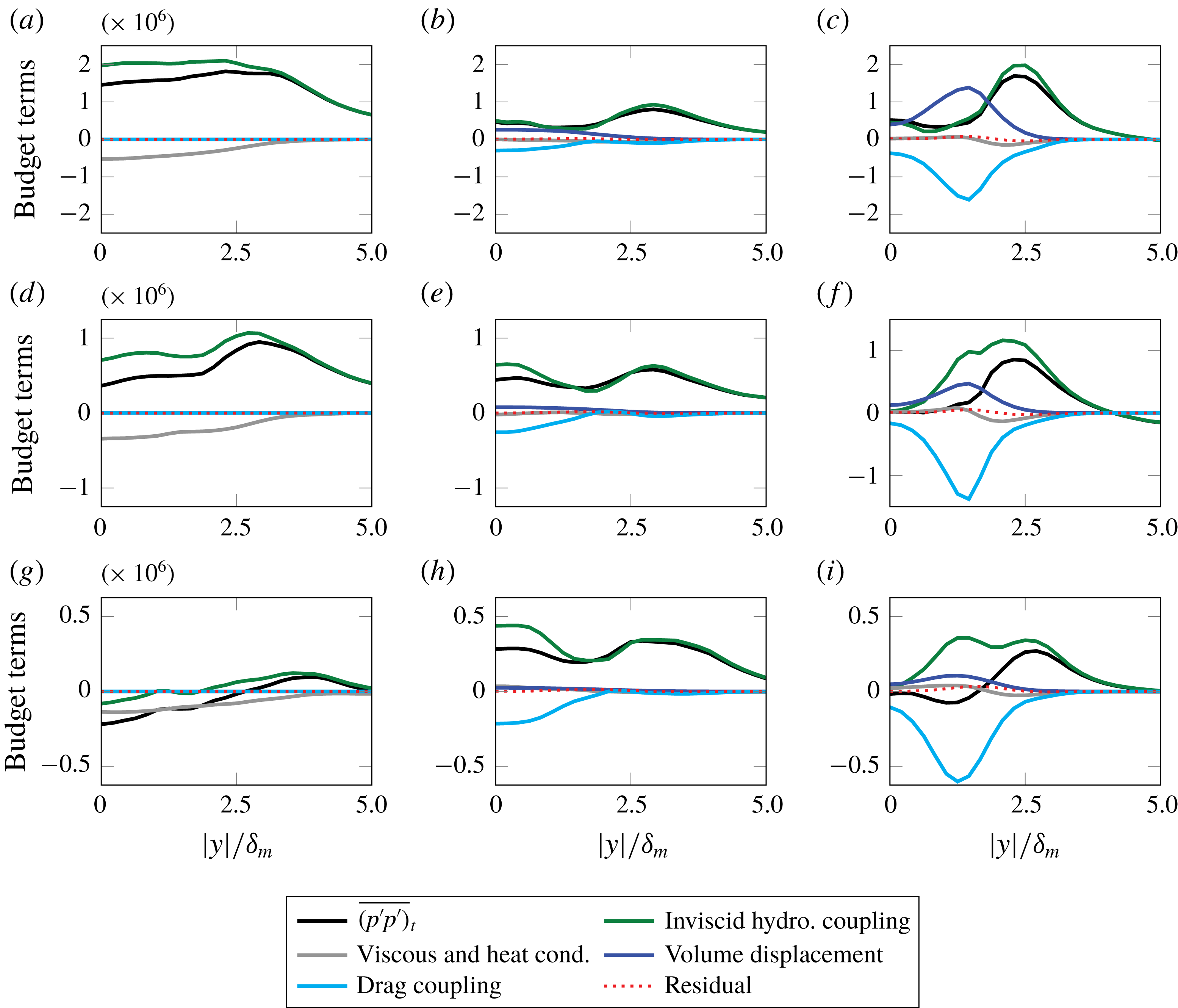
Figure 11. Mechanisms of pressure intensity transport: (a–c)
 $M=0.9$
, (d–f)
$M=0.9$
, (d–f)
 $M=1.5$
and (g–i)
$M=1.5$
and (g–i)
 $M=2.5$
for (a,d,g)
$M=2.5$
for (a,d,g)
 $\unicode[STIX]{x1D6F7}_{m}=0$
, (b,e,h)
$\unicode[STIX]{x1D6F7}_{m}=0$
, (b,e,h)
 $\unicode[STIX]{x1D6F7}_{m}=1$
and (c,f,i)
$\unicode[STIX]{x1D6F7}_{m}=1$
and (c,f,i)
 $\unicode[STIX]{x1D6F7}_{m}=10$
. All components have been scaled by
$\unicode[STIX]{x1D6F7}_{m}=10$
. All components have been scaled by
 $\unicode[STIX]{x1D6FF}_{w}^{o}/(\unicode[STIX]{x1D70C}_{\infty }^{2}\unicode[STIX]{x0394}U^{5})$
. Note the
$\unicode[STIX]{x1D6FF}_{w}^{o}/(\unicode[STIX]{x1D70C}_{\infty }^{2}\unicode[STIX]{x0394}U^{5})$
. Note the
 $y$
-scale changes with respect to Mach number.
$y$
-scale changes with respect to Mach number.
4.3 Near-field pressure fluctuations
Sound fields and turbulence of laden and unladen simulations are shown in figure 12. As the Mach number increases, the waves above the turbulence (depicted with
 $\unicode[STIX]{x1D735}\boldsymbol{\cdot }\boldsymbol{u}$
) are more intense. For supersonic flows, the waves appear sharper and angled, consistent with Mach wave radiation (Phillips Reference Phillips1960; Laufer Reference Laufer1961; Ffowcs Williams & Maidanik Reference Ffowcs Williams and Maidanik1965). For similar single-phase temporally developing shear layers, wave angle statistics with
$\unicode[STIX]{x1D735}\boldsymbol{\cdot }\boldsymbol{u}$
) are more intense. For supersonic flows, the waves appear sharper and angled, consistent with Mach wave radiation (Phillips Reference Phillips1960; Laufer Reference Laufer1961; Ffowcs Williams & Maidanik Reference Ffowcs Williams and Maidanik1965). For similar single-phase temporally developing shear layers, wave angle statistics with
 $M$
have been quantified elsewhere (Buchta & Freund Reference Buchta and Freund2017). For
$M$
have been quantified elsewhere (Buchta & Freund Reference Buchta and Freund2017). For
 $M\gtrsim 1.5$
and
$M\gtrsim 1.5$
and
 $\unicode[STIX]{x1D6F7}_{m}=1$
, the waves above the turbulence (
$\unicode[STIX]{x1D6F7}_{m}=1$
, the waves above the turbulence (
 $y\lesssim 10\unicode[STIX]{x1D6FF}_{m}$
) are fewer and appear smoother than
$y\lesssim 10\unicode[STIX]{x1D6FF}_{m}$
) are fewer and appear smoother than
 $\unicode[STIX]{x1D6F7}_{m}=0$
. Changes in the vorticity magnitude are also apparent and show a decrease with particle loading, which is quantified in figure 10.
$\unicode[STIX]{x1D6F7}_{m}=0$
. Changes in the vorticity magnitude are also apparent and show a decrease with particle loading, which is quantified in figure 10.

Figure 12. Dilatation (greys) shown in the range
 $-0.005<\unicode[STIX]{x1D735}\boldsymbol{\cdot }\boldsymbol{u}\unicode[STIX]{x1D6FF}_{w}^{o}/\unicode[STIX]{x0394}U<0.005$
and vorticity magnitude (colour) in the range
$-0.005<\unicode[STIX]{x1D735}\boldsymbol{\cdot }\boldsymbol{u}\unicode[STIX]{x1D6FF}_{w}^{o}/\unicode[STIX]{x0394}U<0.005$
and vorticity magnitude (colour) in the range
 $|\unicode[STIX]{x1D735}\times \boldsymbol{u}|\unicode[STIX]{x1D6FF}_{w}^{o}/\unicode[STIX]{x0394}U<0.4$
at
$|\unicode[STIX]{x1D735}\times \boldsymbol{u}|\unicode[STIX]{x1D6FF}_{w}^{o}/\unicode[STIX]{x0394}U<0.4$
at
 $z=L_{z}/2$
mid-plane for
$z=L_{z}/2$
mid-plane for
 $\unicode[STIX]{x1D6F7}_{m}=0$
(a,c,e) and
$\unicode[STIX]{x1D6F7}_{m}=0$
(a,c,e) and
 $\unicode[STIX]{x1D6F7}_{m}=1$
(b,d,f) when
$\unicode[STIX]{x1D6F7}_{m}=1$
(b,d,f) when
 $\unicode[STIX]{x1D6FF}_{m}/\unicode[STIX]{x1D6FF}_{m}^{o}=20$
. Unladen (left) and laden (right), with Mach number increasing from top to bottom: (a,b)
$\unicode[STIX]{x1D6FF}_{m}/\unicode[STIX]{x1D6FF}_{m}^{o}=20$
. Unladen (left) and laden (right), with Mach number increasing from top to bottom: (a,b)
 $M=0.9$
, (c,d)
$M=0.9$
, (c,d)
 $M=1.5$
and (e,f)
$M=1.5$
and (e,f)
 $M=2.9$
. Compressions,
$M=2.9$
. Compressions,
 $\unicode[STIX]{x1D735}\boldsymbol{\cdot }\boldsymbol{u}<0$
, are shown in white. To highlight turbulence changes between left and right columns, particle positions are omitted in (b,d,f), and approximately one third of the full
$\unicode[STIX]{x1D735}\boldsymbol{\cdot }\boldsymbol{u}<0$
, are shown in white. To highlight turbulence changes between left and right columns, particle positions are omitted in (b,d,f), and approximately one third of the full
 $y$
-domain is shown.
$y$
-domain is shown.
Sound field changes are likewise shown by instantaneous, pressure fluctuations in figure 13. The subsonic case
 $(M,\unicode[STIX]{x1D6F7}_{m})=(0.9,10)$
shows a large increase in amplitude and appears at shorter wavelengths. For
$(M,\unicode[STIX]{x1D6F7}_{m})=(0.9,10)$
shows a large increase in amplitude and appears at shorter wavelengths. For
 $M=2.5$
, the largest pressure peaks near the shock-like waves appear to decrease. These observations in the pressure trace concur with spectral changes that will be examined next.
$M=2.5$
, the largest pressure peaks near the shock-like waves appear to decrease. These observations in the pressure trace concur with spectral changes that will be examined next.

Figure 13. Mass loading effects on pressure variation in
 $x$
for the subsonic and supersonic shear layers at
$x$
for the subsonic and supersonic shear layers at
 $(y,z)=(15,0)\;\unicode[STIX]{x1D6FF}_{m}$
when (a)
$(y,z)=(15,0)\;\unicode[STIX]{x1D6FF}_{m}$
when (a)
 $\unicode[STIX]{x1D6FF}_{m}/\unicode[STIX]{x1D6FF}_{m}^{o}=20$
for
$\unicode[STIX]{x1D6FF}_{m}/\unicode[STIX]{x1D6FF}_{m}^{o}=20$
for
 $M=0.9$
and when (b)
$M=0.9$
and when (b)
 $\unicode[STIX]{x1D6FF}_{m}/\unicode[STIX]{x1D6FF}_{m}^{o}=30$
for
$\unicode[STIX]{x1D6FF}_{m}/\unicode[STIX]{x1D6FF}_{m}^{o}=30$
for
 $M=2.5$
.
$M=2.5$
.
The effect of particle–turbulence interactions on the spectral components of near-field pressure are shown in figure 14. With increasing Mach number, the spectrum broadens due to the Mach wave radiation mechanism (Laufer, Schlinker & Kaplan Reference Laufer, Schlinker and Kaplan1976); Mach-like waves are indeed apparent in visualizations provided in figure 12(c–f). The universal decrease observed in the mid-plane pressure spectra with the addition of particles (see figure 8) does not hold for the pressure outside of the turbulence, suggesting that a source-to-sound decomposition is not straightforward for
 $M\lesssim 1.5$
. The subsonic case shows an increase in spectral components and slight spectral broadening while
$M\lesssim 1.5$
. The subsonic case shows an increase in spectral components and slight spectral broadening while
 $M=2.5$
shows the opposite effect which has implications for perceived sound levels. The perceived sound field changes from
$M=2.5$
shows the opposite effect which has implications for perceived sound levels. The perceived sound field changes from
 $M=2.5$
might be significant if the Mach wave radiation is reduced, as evidenced by the reduction of
$M=2.5$
might be significant if the Mach wave radiation is reduced, as evidenced by the reduction of
 $E_{p}$
for wavenumbers
$E_{p}$
for wavenumbers
 $5\lesssim k_{x}\unicode[STIX]{x1D6FF}_{m}\lesssim 40$
.
$5\lesssim k_{x}\unicode[STIX]{x1D6FF}_{m}\lesssim 40$
.

Figure 14. (a,c,e) Streamwise and (b,d,f) spanwise pressure spectra, respectively, at
 $y=20\unicode[STIX]{x1D6FF}_{m}$
when
$y=20\unicode[STIX]{x1D6FF}_{m}$
when
 $\unicode[STIX]{x1D6FF}_{m}/\unicode[STIX]{x1D6FF}_{m}^{o}=20$
: (a,b)
$\unicode[STIX]{x1D6FF}_{m}/\unicode[STIX]{x1D6FF}_{m}^{o}=20$
: (a,b)
 $M=0.9$
, (c,d)
$M=0.9$
, (c,d)
 $M=1.5$
and (e,f)
$M=1.5$
and (e,f)
 $M=2.5$
. All spectral components are normalized by
$M=2.5$
. All spectral components are normalized by
 $\unicode[STIX]{x0394}U^{4}\unicode[STIX]{x1D70C}_{\infty }^{2}\unicode[STIX]{x1D6FF}_{m}$
.
$\unicode[STIX]{x0394}U^{4}\unicode[STIX]{x1D70C}_{\infty }^{2}\unicode[STIX]{x1D6FF}_{m}$
.
To quantify the changes in sound pressure levels, figure 15(a) shows the decibel difference, based on average pressure intensity, with respect to the unladen (
 $\unicode[STIX]{x1D6F7}_{m}=0$
) cases as defined by
$\unicode[STIX]{x1D6F7}_{m}=0$
) cases as defined by
 $$\begin{eqnarray}\displaystyle \unicode[STIX]{x0394}\text{SPL}(y,t)=10\log _{10}\left(\frac{\overline{p^{\prime }p^{\prime }}(y,t,\unicode[STIX]{x1D6F7}_{m})}{\overline{p^{\prime }p^{\prime }}(y,t,\unicode[STIX]{x1D6F7}_{m}=0)}\right), & & \displaystyle\end{eqnarray}$$
taken at
 $y=20\unicode[STIX]{x1D6FF}_{m}$
. A similar quantity for the degree of sound reduction in jet turbulence has been used previously (Papamoschou Reference Papamoschou2000). For (4.1), negative values of
$y=20\unicode[STIX]{x1D6FF}_{m}$
. A similar quantity for the degree of sound reduction in jet turbulence has been used previously (Papamoschou Reference Papamoschou2000). For (4.1), negative values of
 $\unicode[STIX]{x0394}\text{SPL}$
indicate sound level reduction relative to the baseline. The sound field changes in figure 15(a) are observed to have Mach number and mass loading dependence. For Mach numbers
$\unicode[STIX]{x0394}\text{SPL}$
indicate sound level reduction relative to the baseline. The sound field changes in figure 15(a) are observed to have Mach number and mass loading dependence. For Mach numbers
 $M\gtrsim 1.5$
, sound reduction is observed for
$M\gtrsim 1.5$
, sound reduction is observed for
 $\unicode[STIX]{x1D6F7}_{m}\gtrsim 1$
, which is consistent with previous experimental observations (Krothapalli et al.
Reference Krothapalli, Venkatakrishnan, Lourenco, Greska and Elavarasan2003; Greska Reference Greska2005). Contrasting this, subsonic flows show a sound level increase with mass loading, by as much as
$\unicode[STIX]{x1D6F7}_{m}\gtrsim 1$
, which is consistent with previous experimental observations (Krothapalli et al.
Reference Krothapalli, Venkatakrishnan, Lourenco, Greska and Elavarasan2003; Greska Reference Greska2005). Contrasting this, subsonic flows show a sound level increase with mass loading, by as much as
 ${\approx}$
6 dB. These observations occur despite universal decrease in the mid-plane average turbulent kinetic energy as quantified in figure 15(b). In the following section, possible mechanisms for the observed sound changes, especially the sound level increase for
${\approx}$
6 dB. These observations occur despite universal decrease in the mid-plane average turbulent kinetic energy as quantified in figure 15(b). In the following section, possible mechanisms for the observed sound changes, especially the sound level increase for
 $M=0.9$
, are considered.
$M=0.9$
, are considered.

Figure 15. (a) Sound pressure level change at
 $y/\unicode[STIX]{x1D6FF}_{m}=20$
and (b) reduction in turbulence level at
$y/\unicode[STIX]{x1D6FF}_{m}=20$
and (b) reduction in turbulence level at
 $y/\unicode[STIX]{x1D6FF}_{m}=0$
. All data are presented for
$y/\unicode[STIX]{x1D6FF}_{m}=0$
. All data are presented for
 $St=1$
.
$St=1$
.
4.4 A pithy discussion of
$\unicode[STIX]{x0394}\text{SPL}$
and low-speed aeroacoustics theory

Crighton & Ffowcs Williams (Reference Crighton and Ffowcs Williams1969) provided a theoretical prediction for sound changes in two-phase turbulence using Lighthill’s acoustic analogy framework. Instead of sound reduction, which was later observed in high-speed jets (Krothapalli et al. Reference Krothapalli, Venkatakrishnan, Lourenco, Greska and Elavarasan2003), their theory predicted enhancement of sound radiation: up to 70 dB increase for air bubbles in water and up to 20 dB increase for solid particles in air. Based on their theory, the largest sound modification was linked to increasing the mixture density by the mass fraction
 $$\begin{eqnarray}\displaystyle \unicode[STIX]{x1D70C}_{m}=\unicode[STIX]{x1D70C}(1+\unicode[STIX]{x1D6F7}_{m}), & & \displaystyle\end{eqnarray}$$
which affects the speed of sound ratio between the disperse-phase–fluid mixture (
 $c_{m}$
) and the fluid phase (
$c_{m}$
) and the fluid phase (
 $c_{\infty }$
)
$c_{\infty }$
)
 $$\begin{eqnarray}\displaystyle \left(\frac{c_{m}}{c_{\infty }}\right)^{2}=\frac{1}{(1+\unicode[STIX]{x1D6F7}_{m})}. & & \displaystyle\end{eqnarray}$$
Without presenting the full details of the formulation, which is a consequence of the governing equations (i.e. mass and momentum conservation), the acoustic efficiency is
 $$\begin{eqnarray}\displaystyle \unicode[STIX]{x1D702}=\frac{{\mathcal{I}}}{\unicode[STIX]{x1D70C}U^{4}L^{2}}\sim \frac{1}{4\unicode[STIX]{x03C0}}(\text{TKE}^{1/2}M)^{5}\left(\frac{c_{\infty }}{c_{m}}\right)^{c}\left(\frac{L}{l_{o}}\right), & & \displaystyle\end{eqnarray}$$
with
 ${\mathcal{I}}$
the acoustic intensity,
${\mathcal{I}}$
the acoustic intensity,
 $U=\unicode[STIX]{x0394}U$
for shear layers,
$U=\unicode[STIX]{x0394}U$
for shear layers,
 $L$
the large-scale length,
$L$
the large-scale length,
 $l_{o}$
the turbulence length scale and the power
$l_{o}$
the turbulence length scale and the power
 $c$
of the speed of sound ratio depends on the mass loading. The efficiency increases from the sound-speed ratio depending on the mass loading with power
$c$
of the speed of sound ratio depends on the mass loading. The efficiency increases from the sound-speed ratio depending on the mass loading with power
 $c=6$
for
$c=6$
for
 $\unicode[STIX]{x1D6F7}_{m}>1$
and
$\unicode[STIX]{x1D6F7}_{m}>1$
and
 $c=2$
for
$c=2$
for
 $\unicode[STIX]{x1D6F7}_{m}<1$
(Crighton & Ffowcs Williams Reference Crighton and Ffowcs Williams1969). It also scales with
$\unicode[STIX]{x1D6F7}_{m}<1$
(Crighton & Ffowcs Williams Reference Crighton and Ffowcs Williams1969). It also scales with
 $M^{5}$
, consistent with the expected behaviour for single-phase flow (Lighthill Reference Lighthill1952). For large mass loadings
$M^{5}$
, consistent with the expected behaviour for single-phase flow (Lighthill Reference Lighthill1952). For large mass loadings
 $\unicode[STIX]{x1D6F7}_{m}>1$
, the acoustic intensity is
$\unicode[STIX]{x1D6F7}_{m}>1$
, the acoustic intensity is
 ${\mathcal{I}}\propto (c_{\infty }/c_{m})^{8}$
using (4.3), which assumes that the scales of turbulence (intensity and length) and mean driving velocity (
${\mathcal{I}}\propto (c_{\infty }/c_{m})^{8}$
using (4.3), which assumes that the scales of turbulence (intensity and length) and mean driving velocity (
 $U$
) are independent of mass loading. Figure 16 shows that the theory overpredicts
$U$
) are independent of mass loading. Figure 16 shows that the theory overpredicts
 $\unicode[STIX]{x0394}\text{SPL}$
compared to the
$\unicode[STIX]{x0394}\text{SPL}$
compared to the
 $M=0.9$
shear-flow turbulence, which was chosen as a candidate to compare with the low-speed theory. Although there are relatively modest changes to the mean flow
$M=0.9$
shear-flow turbulence, which was chosen as a candidate to compare with the low-speed theory. Although there are relatively modest changes to the mean flow
 $\overline{u}(y)$
and energetic scales (see § 4), the particle-laden flow turbulence intensity decreases with
$\overline{u}(y)$
and energetic scales (see § 4), the particle-laden flow turbulence intensity decreases with
 $\unicode[STIX]{x1D6F7}_{m}$
, shown in figure 15(b), which is one cause for discrepancy with the theory. Including the relative turbulence intensity effect and using
$\unicode[STIX]{x1D6F7}_{m}$
, shown in figure 15(b), which is one cause for discrepancy with the theory. Including the relative turbulence intensity effect and using
 $\unicode[STIX]{x0394}\text{SPL}$
in (4.1) yields a modified estimate
$\unicode[STIX]{x0394}\text{SPL}$
in (4.1) yields a modified estimate
 $$\begin{eqnarray}\displaystyle \unicode[STIX]{x0394}\text{SPL}\sim 10\log _{10}\left[(1+\unicode[STIX]{x1D6F7}_{m})^{a}\left(\frac{\text{TKE}}{\text{TKE}_{o}}\right)^{b/2}\right], & & \displaystyle\end{eqnarray}$$
where
 $(a,b)=(4,5)$
for
$(a,b)=(4,5)$
for
 $\unicode[STIX]{x1D6F7}_{m}>1$
and
$\unicode[STIX]{x1D6F7}_{m}>1$
and
 $(a,b)=(2,5)$
for
$(a,b)=(2,5)$
for
 $\unicode[STIX]{x1D6F7}_{m}<1$
, respectively. This modification trends closer to the
$\unicode[STIX]{x1D6F7}_{m}<1$
, respectively. This modification trends closer to the
 $M=0.9$
simulation in figure 16. Note that setting
$M=0.9$
simulation in figure 16. Note that setting
 $b=0$
in (4.5) yields the original expectation of Crighton & Ffowcs Williams (Reference Crighton and Ffowcs Williams1969) for which turbulence intensity is assumed
$b=0$
in (4.5) yields the original expectation of Crighton & Ffowcs Williams (Reference Crighton and Ffowcs Williams1969) for which turbulence intensity is assumed
 $\unicode[STIX]{x1D6F7}_{m}$
-independent. For
$\unicode[STIX]{x1D6F7}_{m}$
-independent. For
 $\unicode[STIX]{x1D6F7}_{m}<1$
, the increase in sound is much less significant following
$\unicode[STIX]{x1D6F7}_{m}<1$
, the increase in sound is much less significant following
 ${\mathcal{I}}\propto (1+\unicode[STIX]{x1D6F7}_{m})^{2}$
and the effect of turbulence modification small since
${\mathcal{I}}\propto (1+\unicode[STIX]{x1D6F7}_{m})^{2}$
and the effect of turbulence modification small since
 $\text{TKE}/\text{TKE}_{o}\approx 1$
for very small mass loadings (
$\text{TKE}/\text{TKE}_{o}\approx 1$
for very small mass loadings (
 $\unicode[STIX]{x1D6F7}_{m}<0.1$
), which is consistent with expectation and simulations for which
$\unicode[STIX]{x1D6F7}_{m}<0.1$
), which is consistent with expectation and simulations for which
 $\unicode[STIX]{x1D6F7}_{m}\ll 1$
has little effect on the sound. Improvements can still be made since the Crighton & Ffowcs Williams (Reference Crighton and Ffowcs Williams1969) theory omits turbulence convection effects and assumes sources are acoustically compact. Although this is a reasonable approximation for
$\unicode[STIX]{x1D6F7}_{m}\ll 1$
has little effect on the sound. Improvements can still be made since the Crighton & Ffowcs Williams (Reference Crighton and Ffowcs Williams1969) theory omits turbulence convection effects and assumes sources are acoustically compact. Although this is a reasonable approximation for
 $M\ll 1$
, at high-speed, turbulence convection affects acoustic efficiency (Ffowcs Williams Reference Ffowcs Williams1963). Furthermore, the theory also assumes that the particles exactly follow the flow (i.e.
$M\ll 1$
, at high-speed, turbulence convection affects acoustic efficiency (Ffowcs Williams Reference Ffowcs Williams1963). Furthermore, the theory also assumes that the particles exactly follow the flow (i.e.
 $\boldsymbol{u}_{p}=\boldsymbol{u}_{f}$
) and that the volume displacement due to particles is small. Based on the local pressure intensity budget in figure 11(c,f,i), volume displacement effects and drag coupling due to local slip velocity
$\boldsymbol{u}_{p}=\boldsymbol{u}_{f}$
) and that the volume displacement due to particles is small. Based on the local pressure intensity budget in figure 11(c,f,i), volume displacement effects and drag coupling due to local slip velocity
 $|\boldsymbol{u}_{p}-\boldsymbol{u}_{f}|>0$
are sizable sources and sinks. Although, their combined causal effect in retarded time on the radiated acoustic intensity remains to be seen. In the current framework, a flow closer to what Crighton & Ffowcs Williams (Reference Crighton and Ffowcs Williams1969) envisioned, for
$|\boldsymbol{u}_{p}-\boldsymbol{u}_{f}|>0$
are sizable sources and sinks. Although, their combined causal effect in retarded time on the radiated acoustic intensity remains to be seen. In the current framework, a flow closer to what Crighton & Ffowcs Williams (Reference Crighton and Ffowcs Williams1969) envisioned, for
 $M\ll 1$
, could be designed by reducing the particle diameter so that
$M\ll 1$
, could be designed by reducing the particle diameter so that
 $\unicode[STIX]{x1D6F7}_{v}\ll 1$
and
$\unicode[STIX]{x1D6F7}_{v}\ll 1$
and
 $St\ll 1$
. However, the computational cost to maintain
$St\ll 1$
. However, the computational cost to maintain
 $0.1<\unicode[STIX]{x1D6F7}_{m}<10$
, reducing
$0.1<\unicode[STIX]{x1D6F7}_{m}<10$
, reducing
 $d_{p}$
, would be significant and outside the scope of the paper for which finite-sized, inertial particles, based on water droplets, in high-speed turbulence are of interest. Thus, a direct comparison to the Crighton & Ffowcs Williams (Reference Crighton and Ffowcs Williams1969) theory was not made beyond this, nor for situations extending beyond the low-speed theory. In a
$d_{p}$
, would be significant and outside the scope of the paper for which finite-sized, inertial particles, based on water droplets, in high-speed turbulence are of interest. Thus, a direct comparison to the Crighton & Ffowcs Williams (Reference Crighton and Ffowcs Williams1969) theory was not made beyond this, nor for situations extending beyond the low-speed theory. In a
 $M\gg 1$
limit, there are additional important effects (e.g. non-compactness of acoustic sources).
$M\gg 1$
limit, there are additional important effects (e.g. non-compactness of acoustic sources).

Figure 16. Models of low-speed sound modulation compared to the
 $M=0.9$
case:
$M=0.9$
case:
 $\unicode[STIX]{x1D6F7}_{m}\gtrsim 1$
models in red and
$\unicode[STIX]{x1D6F7}_{m}\gtrsim 1$
models in red and
 $\unicode[STIX]{x1D6F7}_{m}\lesssim 1$
models in blue. Factors
$\unicode[STIX]{x1D6F7}_{m}\lesssim 1$
models in blue. Factors
 $a$
(
$a$
(
 $\unicode[STIX]{x1D6F7}_{m}$
effect) and
$\unicode[STIX]{x1D6F7}_{m}$
effect) and
 $b$
(TKE effect) apply to equation (4.5): original model neglected TKE modulation (
$b$
(TKE effect) apply to equation (4.5): original model neglected TKE modulation (
 $b=0$
).
$b=0$
).
As discussed, particles in high-speed shear flows can affect the sound radiation by sound-speed effects (
 $c_{m}$
due to
$c_{m}$
due to
 $\unicode[STIX]{x1D6F7}_{m}$
) and due to turbulence changes. For micro-jet injection into round jets, data show that the sound-speed effect is weak; that is, sound radiation for micro-jet gas injection (with gas sound speed approximately equal to the jet) is similar to that of liquid micro-droplet injection (Greska Reference Greska2005), which supports a primary hydrodynamic effect for sound changes. Likewise, in the current simulations, which do not account for speed of sound effects, viz., a mixture equation of state in (4.3), the changes in sound intensity are due to changes in the nature of the turbulence and to additional sound sources from particle interactions.
$\unicode[STIX]{x1D6F7}_{m}$
) and due to turbulence changes. For micro-jet injection into round jets, data show that the sound-speed effect is weak; that is, sound radiation for micro-jet gas injection (with gas sound speed approximately equal to the jet) is similar to that of liquid micro-droplet injection (Greska Reference Greska2005), which supports a primary hydrodynamic effect for sound changes. Likewise, in the current simulations, which do not account for speed of sound effects, viz., a mixture equation of state in (4.3), the changes in sound intensity are due to changes in the nature of the turbulence and to additional sound sources from particle interactions.
For subsonic flows, sound changes can come from subtle modifications to the turbulence; the time rate of change of the eddies leads to sound radiation (e.g. Crighton Reference Crighton1975). Thus, the turbulence sources, based on its dilatation and rate of changes, are shown in figure 17 since they can provide sources of sound (Ribner Reference Ribner1962; Ristorcelli Reference Ristorcelli1997). In the turbulence, the rate of dilatation changes in the
 $M=0.9$
case in figure 17(b) increases, by over an order of magnitude in the domain, due to the presence of particles, which can provide a source to its increased radiated
$M=0.9$
case in figure 17(b) increases, by over an order of magnitude in the domain, due to the presence of particles, which can provide a source to its increased radiated
 $\overline{p^{\prime }p^{\prime }}$
beyond
$\overline{p^{\prime }p^{\prime }}$
beyond
 $y\gtrsim 5~\unicode[STIX]{x1D6FF}_{m}$
. For
$y\gtrsim 5~\unicode[STIX]{x1D6FF}_{m}$
. For
 $M=2.5$
in figure 17(f), these rates of change are already large for
$M=2.5$
in figure 17(f), these rates of change are already large for
 $\unicode[STIX]{x1D6F7}_{m}=0$
so the effect of particles, beyond that of the baseline turbulence, is relatively small. The
$\unicode[STIX]{x1D6F7}_{m}=0$
so the effect of particles, beyond that of the baseline turbulence, is relatively small. The
 $M=2.5$
sound changes can be linked to the domain-wide decrease in dilatation (and turbulence decrease), shown in figure 17(e), which concurs with its decrease in sound intensity. Similar observations for dilatation were made from particle-laden supersonic convecting spatially developing turbulence simulations for
$M=2.5$
sound changes can be linked to the domain-wide decrease in dilatation (and turbulence decrease), shown in figure 17(e), which concurs with its decrease in sound intensity. Similar observations for dilatation were made from particle-laden supersonic convecting spatially developing turbulence simulations for
 $\unicode[STIX]{x1D6F7}_{m}=0.5$
(Dai et al.
Reference Dai, Jin, Luo and Fan2018).
$\unicode[STIX]{x1D6F7}_{m}=0.5$
(Dai et al.
Reference Dai, Jin, Luo and Fan2018).
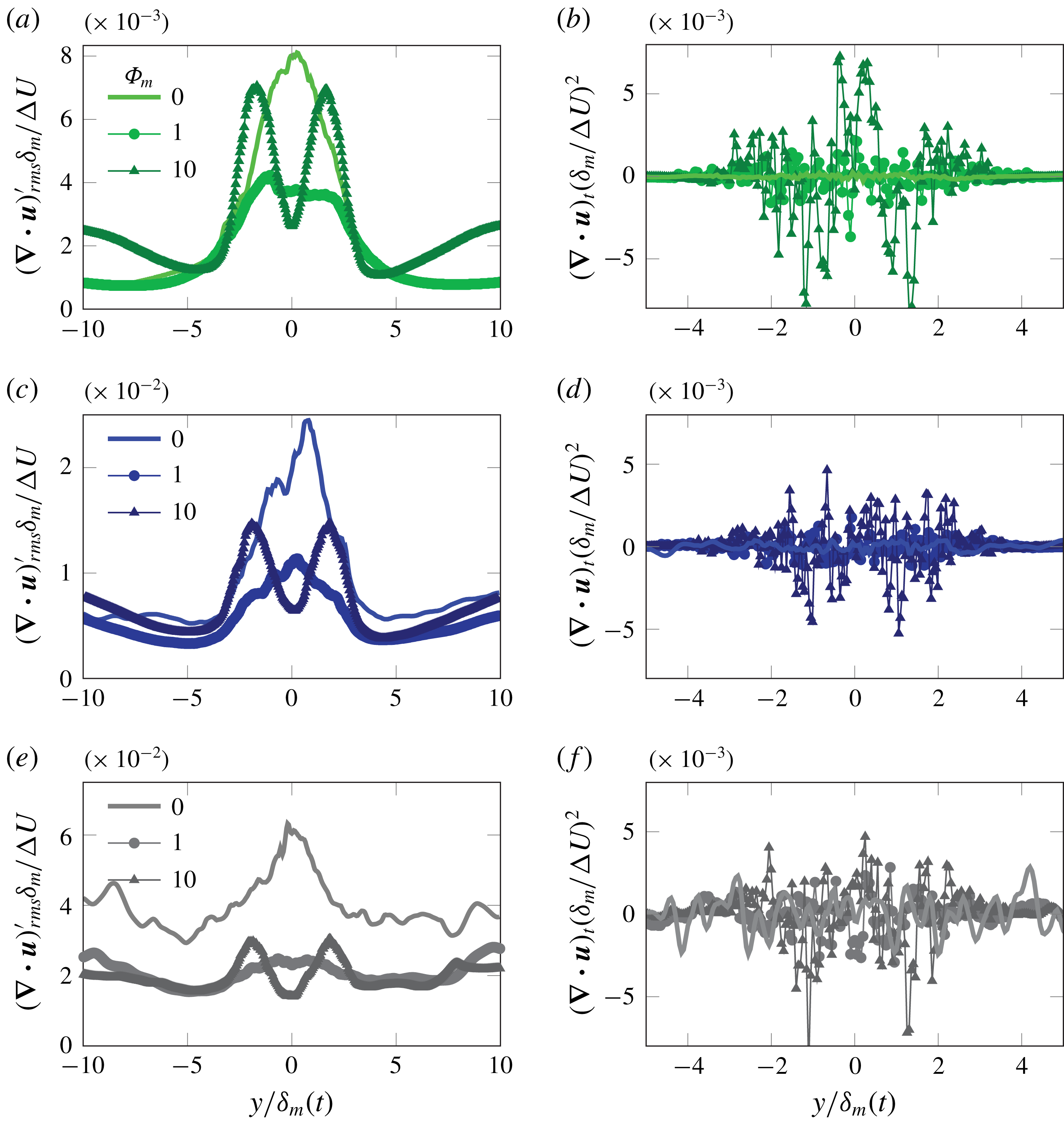
Figure 17. (a,c,e) Average fluctuating dilatation and (b,d,f) average instantaneous rate of change of dilatation when
 $\unicode[STIX]{x1D6FF}_{m}/\unicode[STIX]{x1D6FF}_{m}^{o}=20$
: (a,b)
$\unicode[STIX]{x1D6FF}_{m}/\unicode[STIX]{x1D6FF}_{m}^{o}=20$
: (a,b)
 $M=0.9$
, (c,d)
$M=0.9$
, (c,d)
 $M=1.5$
and (e,f)
$M=1.5$
and (e,f)
 $M=2.5$
.
$M=2.5$
.
5 Conclusions and discussion
Numerical simulations of particle-laden high-speed planar shear-flow turbulence are used to examine the particle–turbulence coupling effects on velocity and pressure fluctuations. Interphase coupling has a broadband effect on the turbulence and pressure fields – reducing the turbulence by over
 $70\,\%$
for mass loading
$70\,\%$
for mass loading
 $\unicode[STIX]{x1D6F7}_{m}=10$
. Analysis of pressure intensity transport mechanisms show that changes in the intensity follow primarily from changes to the turbulence. Local pressure intensity sources and sinks from volume displacement and drag coupling, respectively, are only substantial for
$\unicode[STIX]{x1D6F7}_{m}=10$
. Analysis of pressure intensity transport mechanisms show that changes in the intensity follow primarily from changes to the turbulence. Local pressure intensity sources and sinks from volume displacement and drag coupling, respectively, are only substantial for
 $\unicode[STIX]{x1D6F7}_{m}\gtrsim 1$
. For subsonic shear layers (
$\unicode[STIX]{x1D6F7}_{m}\gtrsim 1$
. For subsonic shear layers (
 $M=0.9$
), these two effects approximately cancel, obfuscating possible mechanisms for their near-field sound changes; however, significant changes to fluid dilatation rates (with
$M=0.9$
), these two effects approximately cancel, obfuscating possible mechanisms for their near-field sound changes; however, significant changes to fluid dilatation rates (with
 $\unicode[STIX]{x1D6F7}_{m}$
) indicate a potential mechanism for increasing net sound radiation for
$\unicode[STIX]{x1D6F7}_{m}$
) indicate a potential mechanism for increasing net sound radiation for
 $\unicode[STIX]{x1D6F7}_{m}\gtrsim 1$
. These results motivate alternative descriptions of sound-reducing mechanisms and source-to-sound decompositions for guiding design, especially for more complex configurations. For example, simplified turbulence source descriptions (e.g. wave packets) may facilitate analysis for the growing–decaying turbulence dynamics which underpin sound radiation in subsonic single-phase flow (Jordan & Colonius Reference Jordan and Colonius2013). Contrasting lower-speed particle-laden flow turbulence simulations, sound radiation decreases with
$\unicode[STIX]{x1D6F7}_{m}\gtrsim 1$
. These results motivate alternative descriptions of sound-reducing mechanisms and source-to-sound decompositions for guiding design, especially for more complex configurations. For example, simplified turbulence source descriptions (e.g. wave packets) may facilitate analysis for the growing–decaying turbulence dynamics which underpin sound radiation in subsonic single-phase flow (Jordan & Colonius Reference Jordan and Colonius2013). Contrasting lower-speed particle-laden flow turbulence simulations, sound radiation decreases with
 $0.1\lesssim \unicode[STIX]{x1D6F7}_{m}\lesssim 10$
for supersonic convection shear layers (
$0.1\lesssim \unicode[STIX]{x1D6F7}_{m}\lesssim 10$
for supersonic convection shear layers (
 $M>1.5$
) as well as a decrease in turbulence and dilatation levels. Modest sound reductions,
$M>1.5$
) as well as a decrease in turbulence and dilatation levels. Modest sound reductions,
 ${\lesssim}$
2 dB for
${\lesssim}$
2 dB for
 $M=2.5$
concur with observations that sound radiation in supersonic flows is relatively insensitive to source changes, for example, due to its turbulence structure (Buchta & Freund Reference Buchta and Freund2019).
$M=2.5$
concur with observations that sound radiation in supersonic flows is relatively insensitive to source changes, for example, due to its turbulence structure (Buchta & Freund Reference Buchta and Freund2019).
Acknowledgements
The authors thank R. Vishnampet for access to his single-phase compressible flow solver and J. Kim for his detailed comments on an earlier draft of the manuscript. A portion of the single-phase simulation framework was developed by D. A. Buchta while a student of Professor Freund at the University of Illinois. This research used resources of the Oak Ridge Leadership Computing Facility at the Oak Ridge National Laboratory, which is supported by the Office of Science of the U.S. Department of Energy under contract no. DE-AC05-00OR22725 through the Director’s Discretionary Program and from the Advanced Research Computing Technology Services at the University of Michigan. Part of this work was supported by a NASA Space Technology Research Fellowship.
Appendix A. Volume filtering the compressible flow equations
This section provides the volume-filtered derivation of the viscous compressible Navier–Stokes equations used in the simulations. Attention is paid to the energy equation as the majority of work to this date has focused on incompressible flows. Here we extend the local averaging procedure of Anderson & Jackson (Reference Anderson and Jackson1967) to the compressible Navier–Stokes equations,
 $$\begin{eqnarray}\displaystyle & \displaystyle \frac{\unicode[STIX]{x2202}\unicode[STIX]{x1D70C}^{\ast }}{\unicode[STIX]{x2202}t}+\unicode[STIX]{x1D735}\boldsymbol{\cdot }(\unicode[STIX]{x1D70C}^{\ast }\boldsymbol{u}^{\ast })=0, & \displaystyle\end{eqnarray}$$
 $$\begin{eqnarray}\displaystyle & \displaystyle \frac{\unicode[STIX]{x2202}\unicode[STIX]{x1D70C}^{\ast }\boldsymbol{u}^{\ast }}{\unicode[STIX]{x2202}t}+\unicode[STIX]{x1D735}\boldsymbol{\cdot }(\unicode[STIX]{x1D70C}^{\ast }\boldsymbol{u}^{\ast }\otimes \boldsymbol{u}^{\ast }+p^{\ast }\mathbb{I}-\unicode[STIX]{x1D749}^{\ast })=0, & \displaystyle\end{eqnarray}$$
and
 $$\begin{eqnarray}\displaystyle \frac{\unicode[STIX]{x2202}\unicode[STIX]{x1D70C}^{\ast }E^{\ast }}{\unicode[STIX]{x2202}t}+\unicode[STIX]{x1D735}\boldsymbol{\cdot }(\{\unicode[STIX]{x1D70C}^{\ast }E^{\ast }+p^{\ast }\}\boldsymbol{u}^{\ast }+\boldsymbol{q}^{\ast }-\boldsymbol{u}^{\ast }\boldsymbol{\cdot }\unicode[STIX]{x1D749}^{\ast })=0, & & \displaystyle\end{eqnarray}$$
where superscript
 $\ast$
indicates a microscale quantity (i.e. a scalar or vector field resolved at the scale of an individual particle), and
$\ast$
indicates a microscale quantity (i.e. a scalar or vector field resolved at the scale of an individual particle), and
 $\mathbb{I}$
is the identity matrix. The relation between microscale pressure and total energy is
$\mathbb{I}$
is the identity matrix. The relation between microscale pressure and total energy is
 $$\begin{eqnarray}\displaystyle p^{\ast }=(\unicode[STIX]{x1D6FE}-1)\left(\unicode[STIX]{x1D70C}^{\ast }E^{\ast }-{\textstyle \frac{1}{2}}\unicode[STIX]{x1D70C}^{\ast }\boldsymbol{u}^{\ast }\boldsymbol{\cdot }\boldsymbol{u}^{\ast }\right). & & \displaystyle\end{eqnarray}$$
Finally, the ideal gas law (in non-dimensional form) is given by
 $$\begin{eqnarray}\displaystyle T^{\ast }=\frac{\unicode[STIX]{x1D6FE}p^{\ast }}{\unicode[STIX]{x1D70C}^{\ast }(\unicode[STIX]{x1D6FE}-1)}. & & \displaystyle\end{eqnarray}$$
In order to account for the effect of particles without requiring to resolve the fluid-phase equations on the scale of the particle surface, the Navier–Stokes equations are split into microscale (particle-scale) processes, and mesoscale processes, i.e. processes that take place on a scale much larger than the particle diameter. To facilitate a description of this length-scale separation, a filtering kernel
 ${\mathcal{G}}$
is used with a characteristic length
${\mathcal{G}}$
is used with a characteristic length
 $\unicode[STIX]{x1D6FF}_{f}$
, such that
$\unicode[STIX]{x1D6FF}_{f}$
, such that
 ${\mathcal{G}}(r)>0$
decreases monotonically with increasing
${\mathcal{G}}(r)>0$
decreases monotonically with increasing
 $r$
, and is normalized such that its integral over the entire physical space is unity. The local voidage at a point
$r$
, and is normalized such that its integral over the entire physical space is unity. The local voidage at a point
 $\boldsymbol{x}$
and time
$\boldsymbol{x}$
and time
 $t$
is defined as
$t$
is defined as
 $$\begin{eqnarray}\displaystyle \unicode[STIX]{x1D6FC}(\boldsymbol{x},t)=\int _{{\mathcal{V}}_{f}}{\mathcal{G}}(|\boldsymbol{x}-\boldsymbol{y}|)\,\text{d}\boldsymbol{y}, & & \displaystyle\end{eqnarray}$$
where
 ${\mathcal{V}}_{f}$
indicates that the integral is taken over all points
${\mathcal{V}}_{f}$
indicates that the integral is taken over all points
 $\boldsymbol{y}$
occupied by the fluid. Due to contributions at the particle surface, there is no commutation between filtering and differentiation. Consequently, filtering derivatives of point variables will lead to additional terms in the form of integrals of the pointwise quantity about the surface of the particle. Volume filtering the gradient, divergence and time derivative of a point property of the fluid
$\boldsymbol{y}$
occupied by the fluid. Due to contributions at the particle surface, there is no commutation between filtering and differentiation. Consequently, filtering derivatives of point variables will lead to additional terms in the form of integrals of the pointwise quantity about the surface of the particle. Volume filtering the gradient, divergence and time derivative of a point property of the fluid
 $\boldsymbol{a}^{\ast }$
are respectively given as
$\boldsymbol{a}^{\ast }$
are respectively given as
 $$\begin{eqnarray}\displaystyle & \displaystyle \int _{{\mathcal{V}}_{f}}\unicode[STIX]{x1D735}\boldsymbol{a}^{\ast }(\boldsymbol{y},t){\mathcal{G}}(|\boldsymbol{x}-\boldsymbol{y}|)\,\text{d}\boldsymbol{y}=\unicode[STIX]{x1D735}(\unicode[STIX]{x1D6FC}\boldsymbol{a}(\boldsymbol{x},t))-\mathop{\sum }_{i=1}^{N_{p}}\int _{{\mathcal{S}}_{i}}\boldsymbol{n}\otimes \boldsymbol{a}^{\ast }(\boldsymbol{y},t){\mathcal{G}}(|\boldsymbol{x}-\boldsymbol{y}|)\,\text{d}\boldsymbol{y},\qquad & \displaystyle\end{eqnarray}$$
 $$\begin{eqnarray}\displaystyle & \displaystyle \int _{{\mathcal{V}}_{f}}\unicode[STIX]{x1D735}\boldsymbol{\cdot }\boldsymbol{a}^{\ast }(\boldsymbol{y},t){\mathcal{G}}(|\boldsymbol{x}-\boldsymbol{y}|)\,\text{d}\boldsymbol{y}=\unicode[STIX]{x1D735}\boldsymbol{\cdot }(\unicode[STIX]{x1D6FC}\boldsymbol{a}(\boldsymbol{x},t))-\mathop{\sum }_{i=1}^{N_{p}}\int _{{\mathcal{S}}_{i}}\boldsymbol{n}\boldsymbol{\cdot }\boldsymbol{a}^{\ast }(\boldsymbol{y},t){\mathcal{G}}(|\boldsymbol{x}-\boldsymbol{y}|)\,\text{d}\boldsymbol{y},\qquad & \displaystyle\end{eqnarray}$$
and
 $$\begin{eqnarray}\displaystyle \int _{{\mathcal{V}}_{f}}\frac{\unicode[STIX]{x2202}\boldsymbol{a}^{\ast }(\boldsymbol{y},t)}{\unicode[STIX]{x2202}t}{\mathcal{G}}(|\boldsymbol{x}-\boldsymbol{y}|)\,\text{d}\boldsymbol{y}=\frac{\unicode[STIX]{x2202}}{\unicode[STIX]{x2202}t}(\unicode[STIX]{x1D6FC}\boldsymbol{a}(\boldsymbol{x},t))+\mathop{\sum }_{i=1}^{N_{p}}\int _{{\mathcal{S}}_{i}}\boldsymbol{n}\boldsymbol{\cdot }\boldsymbol{v}_{p}^{(i)}\boldsymbol{a}^{\ast }(\boldsymbol{y},t){\mathcal{G}}(|\boldsymbol{x}-\boldsymbol{y}|)\,\text{d}\boldsymbol{y},\qquad & & \displaystyle\end{eqnarray}$$
where
 ${\mathcal{S}}_{i}$
represents the surface of particle
${\mathcal{S}}_{i}$
represents the surface of particle
 $i$
,
$i$
,
 $\boldsymbol{n}$
is the unit normal vector outward from the surface of the particle and
$\boldsymbol{n}$
is the unit normal vector outward from the surface of the particle and
 $\boldsymbol{v}_{p}^{(i)}$
is its velocity.
$\boldsymbol{v}_{p}^{(i)}$
is its velocity.
Applying these definitions to the microscale density equation (A 1) yields
 $$\begin{eqnarray}\displaystyle \frac{\unicode[STIX]{x2202}\unicode[STIX]{x1D6FC}\unicode[STIX]{x1D70C}}{\unicode[STIX]{x2202}t}+\unicode[STIX]{x1D735}\boldsymbol{\cdot }(\unicode[STIX]{x1D6FC}\unicode[STIX]{x1D70C}\boldsymbol{u})=0. & & \displaystyle\end{eqnarray}$$
Volume filtering the pressure gradient term in the momentum equation yields
 $$\begin{eqnarray}\displaystyle \int _{{\mathcal{V}}_{f}}\unicode[STIX]{x1D735}p^{\ast }{\mathcal{G}}(|\boldsymbol{x}-\boldsymbol{y}|)\,\text{d}\boldsymbol{y}=\unicode[STIX]{x1D735}(\unicode[STIX]{x1D6FC}p)-\mathop{\sum }_{i=1}^{N_{p}}\int _{{\mathcal{S}}_{i}}\boldsymbol{n}p^{\ast }{\mathcal{G}}(|\boldsymbol{x}-\boldsymbol{y}|)\,\text{d}\boldsymbol{y}, & & \displaystyle\end{eqnarray}$$
where
 $\boldsymbol{n}p^{\ast }$
represents the interfacial pressure. Decomposing the local pressure
$\boldsymbol{n}p^{\ast }$
represents the interfacial pressure. Decomposing the local pressure
 $p^{\ast }=p+p^{\prime }$
, the second term on the right-hand side can be expressed as
$p^{\ast }=p+p^{\prime }$
, the second term on the right-hand side can be expressed as
 $$\begin{eqnarray}\displaystyle \mathop{\sum }_{i=1}^{N_{p}}\int _{{\mathcal{S}}_{i}}\boldsymbol{n}p^{\ast }{\mathcal{G}}(|\boldsymbol{x}-\boldsymbol{y}|)\,\text{d}\boldsymbol{y}=\mathop{\sum }_{i=1}^{N_{p}}\int _{{\mathcal{S}}_{i}}\boldsymbol{n}p{\mathcal{G}}(|\boldsymbol{x}-\boldsymbol{y}|)\,\text{d}\boldsymbol{y}+\mathop{\sum }_{i=1}^{N_{p}}\int _{{\mathcal{S}}_{i}}\boldsymbol{n}p^{\prime }{\mathcal{G}}(|\boldsymbol{x}-\boldsymbol{y}|)\,\text{d}\boldsymbol{y},\qquad & & \displaystyle\end{eqnarray}$$
where the last term involving surface contributions of the sub-filtered pressure
 $p^{\prime }$
is unclosed. Assuming the characteristic size of the filter kernel
$p^{\prime }$
is unclosed. Assuming the characteristic size of the filter kernel
 $\unicode[STIX]{x1D6FF}_{f}\gg d_{p}$
,
$\unicode[STIX]{x1D6FF}_{f}\gg d_{p}$
,
 $p$
varies little over the surface of the particle and can be taken out of the integral of the first term on the right-hand side. Applying the divergence theorem, the volume-filtered pressure gradient can be expressed as
$p$
varies little over the surface of the particle and can be taken out of the integral of the first term on the right-hand side. Applying the divergence theorem, the volume-filtered pressure gradient can be expressed as
 $$\begin{eqnarray}\displaystyle \int _{{\mathcal{V}}_{f}}\unicode[STIX]{x1D735}p^{\ast }{\mathcal{G}}(|\boldsymbol{x}-\boldsymbol{y}|)\,\text{d}\boldsymbol{y}=\unicode[STIX]{x1D735}(\unicode[STIX]{x1D6FC}p)-p\unicode[STIX]{x1D735}\unicode[STIX]{x1D6FC}-\mathop{\sum }_{i=1}^{N_{p}}\int _{{\mathcal{S}}_{i}}\boldsymbol{n}p^{\prime }{\mathcal{G}}(|\boldsymbol{x}-\boldsymbol{y}|)\,\text{d}\boldsymbol{y}, & & \displaystyle\end{eqnarray}$$
where the last term on the right-hand side of (A 13) needs to be modelled. Here,
 $p\unicode[STIX]{x1D735}\unicode[STIX]{x1D6FC}$
represents a nozzling term that accelerates the gas due to particles restricting the area where fluid can flow (Houim & Oran Reference Houim and Oran2016). Applying the same procedure to the viscous stress tensor, the volume-filtered momentum equation can be expressed as
$p\unicode[STIX]{x1D735}\unicode[STIX]{x1D6FC}$
represents a nozzling term that accelerates the gas due to particles restricting the area where fluid can flow (Houim & Oran Reference Houim and Oran2016). Applying the same procedure to the viscous stress tensor, the volume-filtered momentum equation can be expressed as
 $$\begin{eqnarray}\displaystyle \frac{\unicode[STIX]{x2202}\unicode[STIX]{x1D6FC}\unicode[STIX]{x1D70C}\boldsymbol{u}}{\unicode[STIX]{x2202}t}+\unicode[STIX]{x1D735}\boldsymbol{\cdot }(\unicode[STIX]{x1D6FC}\{\unicode[STIX]{x1D70C}\boldsymbol{u}\otimes \boldsymbol{u}+p\mathbb{I}-\unicode[STIX]{x1D749}+\boldsymbol{R}\})=(p\mathbb{I}-\unicode[STIX]{x1D749})\boldsymbol{\cdot }\unicode[STIX]{x1D735}\unicode[STIX]{x1D6FC}+\boldsymbol{F}, & & \displaystyle\end{eqnarray}$$
where
 $\boldsymbol{R}$
is akin to a Reynolds stress in the context of large-eddy simulations (referred to as the pseudo-turbulent Reynolds stress (Mehrabadi et al.
Reference Mehrabadi, Tenneti, Garg and Subramaniam2015)) and contains sub-filtered velocity fluctuations due to, for example, wakes past particles;
$\boldsymbol{R}$
is akin to a Reynolds stress in the context of large-eddy simulations (referred to as the pseudo-turbulent Reynolds stress (Mehrabadi et al.
Reference Mehrabadi, Tenneti, Garg and Subramaniam2015)) and contains sub-filtered velocity fluctuations due to, for example, wakes past particles;
 $\boldsymbol{F}$
represents a sub-filtered momentum exchange term that is typically modelled using drag correlations based on local Reynolds number, Mach number and volume fraction (Clift et al.
Reference Clift, Grace and Weber2005). In low Mach number flows, it is common to simplify the momentum equation by employing the product rule, i.e.
$\boldsymbol{F}$
represents a sub-filtered momentum exchange term that is typically modelled using drag correlations based on local Reynolds number, Mach number and volume fraction (Clift et al.
Reference Clift, Grace and Weber2005). In low Mach number flows, it is common to simplify the momentum equation by employing the product rule, i.e.
 $\unicode[STIX]{x1D735}(\unicode[STIX]{x1D6FC}p)=p\unicode[STIX]{x1D735}\unicode[STIX]{x1D6FC}+\unicode[STIX]{x1D6FC}\unicode[STIX]{x1D735}p$
, such that the non-conservative nozzling term (
$\unicode[STIX]{x1D735}(\unicode[STIX]{x1D6FC}p)=p\unicode[STIX]{x1D735}\unicode[STIX]{x1D6FC}+\unicode[STIX]{x1D6FC}\unicode[STIX]{x1D735}p$
, such that the non-conservative nozzling term (
 $p\unicode[STIX]{x1D735}\unicode[STIX]{x1D6FC}$
) cancels with the first term on the right-hand side of equation (A 14) (Capecelatro & Desjardins Reference Capecelatro and Desjardins2013). Therefore, under the assumption of an incompressible disperse phase, and neglecting
$p\unicode[STIX]{x1D735}\unicode[STIX]{x1D6FC}$
) cancels with the first term on the right-hand side of equation (A 14) (Capecelatro & Desjardins Reference Capecelatro and Desjardins2013). Therefore, under the assumption of an incompressible disperse phase, and neglecting
 $\boldsymbol{R}$
as is typically done in simulations of fluid–particle flows, the momentum equation can be expressed as
$\boldsymbol{R}$
as is typically done in simulations of fluid–particle flows, the momentum equation can be expressed as
 $$\begin{eqnarray}\displaystyle \frac{\unicode[STIX]{x2202}\unicode[STIX]{x1D6FC}\unicode[STIX]{x1D70C}\boldsymbol{u}}{\unicode[STIX]{x2202}t}+\unicode[STIX]{x1D735}\boldsymbol{\cdot }(\unicode[STIX]{x1D6FC}\unicode[STIX]{x1D70C}\boldsymbol{u}\otimes \boldsymbol{u})+\unicode[STIX]{x1D6FC}\unicode[STIX]{x1D735}\boldsymbol{\cdot }(p\mathbb{I}-\unicode[STIX]{x1D749})=\boldsymbol{F}. & & \displaystyle\end{eqnarray}$$
For the gas-phase energy equation (A 3), volume filtering the work done by pressure yields
 $$\begin{eqnarray}\displaystyle \int _{{\mathcal{V}}_{f}}\unicode[STIX]{x1D735}\boldsymbol{\cdot }(p^{\ast }\boldsymbol{u}^{\ast }){\mathcal{G}}(|\boldsymbol{x}-\boldsymbol{y}|)\,\text{d}\boldsymbol{y}=\unicode[STIX]{x1D735}\boldsymbol{\cdot }(\unicode[STIX]{x1D6FC}p\boldsymbol{u})-\mathop{\sum }_{i=1}^{N_{p}}\int _{{\mathcal{S}}_{i}}\boldsymbol{n}\boldsymbol{\cdot }(p^{\ast }\boldsymbol{u}^{\ast }){\mathcal{G}}(|\boldsymbol{x}-\boldsymbol{y}|)\,\text{d}\boldsymbol{y}. & & \displaystyle\end{eqnarray}$$
The fluid-phase velocity at the surface of the particle can be decomposed into
 $\boldsymbol{u}^{\ast }|_{{\mathcal{S}}_{i}}=\boldsymbol{v}_{p}^{(i)}+{\dot{r}}_{p}^{(i)}\boldsymbol{n}$
, where
$\boldsymbol{u}^{\ast }|_{{\mathcal{S}}_{i}}=\boldsymbol{v}_{p}^{(i)}+{\dot{r}}_{p}^{(i)}\boldsymbol{n}$
, where
 ${\dot{r}}_{p}^{(i)}$
is the rate of change of the radius of particle
${\dot{r}}_{p}^{(i)}$
is the rate of change of the radius of particle
 $i$
. Decomposing the pressure into its filtered and sub-filtered contributions, and assuming rigid particles (i.e.
$i$
. Decomposing the pressure into its filtered and sub-filtered contributions, and assuming rigid particles (i.e.
 ${\dot{r}}_{p}=0$
), the last term on the right-hand side of (A 16) becomes
${\dot{r}}_{p}=0$
), the last term on the right-hand side of (A 16) becomes
 $$\begin{eqnarray}\displaystyle & & \displaystyle \mathop{\sum }_{i=1}^{N_{p}}\int _{{\mathcal{S}}_{i}}\boldsymbol{n}\boldsymbol{\cdot }(p^{\ast }\boldsymbol{u}^{\ast }){\mathcal{G}}(|\boldsymbol{x}-\boldsymbol{y}|)\,\text{d}\boldsymbol{y}\nonumber\\ \displaystyle & & \displaystyle \quad =p\mathop{\sum }_{i=1}^{N_{p}}\int _{{\mathcal{S}}_{i}}\boldsymbol{n}\boldsymbol{\cdot }\boldsymbol{v}_{p}^{(i)}{\mathcal{G}}(|\boldsymbol{x}-\boldsymbol{y}|)\,\text{d}\boldsymbol{y}+\mathop{\sum }_{i=1}^{N_{p}}\int _{{\mathcal{S}}_{i}}p^{\prime }\boldsymbol{n}\boldsymbol{\cdot }\boldsymbol{v}_{p}^{(i)}{\mathcal{G}}(|\boldsymbol{x}-\boldsymbol{y}|)\,\text{d}\boldsymbol{y}.\end{eqnarray}$$
Applying (A 9) to the first term on the right-hand side of (A 17) with
 $\boldsymbol{a}^{\ast }=1$
yields
$\boldsymbol{a}^{\ast }=1$
yields
 $$\begin{eqnarray}\displaystyle \int _{{\mathcal{V}}_{f}}\unicode[STIX]{x1D735}\boldsymbol{\cdot }(p^{\ast }\boldsymbol{u}^{\ast }){\mathcal{G}}(|\boldsymbol{x}-\boldsymbol{y}|)\,\text{d}\boldsymbol{y}=\unicode[STIX]{x1D735}\boldsymbol{\cdot }(\unicode[STIX]{x1D6FC}p\boldsymbol{u})+p\frac{\unicode[STIX]{x2202}\unicode[STIX]{x1D6FC}}{\unicode[STIX]{x2202}t}-\mathop{\sum }_{i=1}^{N_{p}}\int _{{\mathcal{S}}_{i}}p^{\prime }\boldsymbol{n}\boldsymbol{\cdot }\boldsymbol{v}_{p}^{(i)}{\mathcal{G}}(|\boldsymbol{x}-\boldsymbol{y}|)\,\text{d}\boldsymbol{y},\qquad & & \displaystyle\end{eqnarray}$$
where
 $p\unicode[STIX]{x2202}\unicode[STIX]{x1D6FC}/\unicode[STIX]{x2202}t$
represents a
$p\unicode[STIX]{x2202}\unicode[STIX]{x1D6FC}/\unicode[STIX]{x2202}t$
represents a
 $pDV$
work term due to particles entering and leaving a control volume (Lhuillier et al.
Reference Lhuillier, Theofanous and Liou2010). Because
$pDV$
work term due to particles entering and leaving a control volume (Lhuillier et al.
Reference Lhuillier, Theofanous and Liou2010). Because
 $\boldsymbol{v}_{p}$
is constant over the surface of the particle, it can be brought outside of the integral in the last term on the right-hand side of equation (A 18), resulting in
$\boldsymbol{v}_{p}$
is constant over the surface of the particle, it can be brought outside of the integral in the last term on the right-hand side of equation (A 18), resulting in
 $\sum _{i=1}^{N_{p}}\boldsymbol{v}_{p}^{(i)}\boldsymbol{\cdot }\int _{{\mathcal{S}}_{i}}p^{\prime }\boldsymbol{n}{\mathcal{G}}(|\boldsymbol{x}-\boldsymbol{y}|)\,\text{d}\boldsymbol{y}$
. This sub-filtered term is now identical to the closure appearing in the momentum equation (A 12) (but multiplied by the particle velocity). As described by Ling, Balachandar & Parmar (Reference Ling, Balachandar and Parmar2016), multiplying
$\sum _{i=1}^{N_{p}}\boldsymbol{v}_{p}^{(i)}\boldsymbol{\cdot }\int _{{\mathcal{S}}_{i}}p^{\prime }\boldsymbol{n}{\mathcal{G}}(|\boldsymbol{x}-\boldsymbol{y}|)\,\text{d}\boldsymbol{y}$
. This sub-filtered term is now identical to the closure appearing in the momentum equation (A 12) (but multiplied by the particle velocity). As described by Ling, Balachandar & Parmar (Reference Ling, Balachandar and Parmar2016), multiplying
 $\boldsymbol{F}$
by the particle velocity ensures the microscale kinetic energy is dissipated and transferred to the internal energy of the fluid. Using a similar procedure for the viscous stress tensor, the volume-filtered energy equation can be expressed as
$\boldsymbol{F}$
by the particle velocity ensures the microscale kinetic energy is dissipated and transferred to the internal energy of the fluid. Using a similar procedure for the viscous stress tensor, the volume-filtered energy equation can be expressed as
 $$\begin{eqnarray}\frac{\unicode[STIX]{x2202}\unicode[STIX]{x1D6FC}\unicode[STIX]{x1D70C}E}{\unicode[STIX]{x2202}t}+\unicode[STIX]{x1D735}\boldsymbol{\cdot }\unicode[STIX]{x1D6FC}(\{\unicode[STIX]{x1D70C}E+p\}\boldsymbol{u}-\boldsymbol{u}\boldsymbol{\cdot }\unicode[STIX]{x1D749})+\unicode[STIX]{x1D6FC}\unicode[STIX]{x1D735}\boldsymbol{\cdot }\boldsymbol{q}=-p\frac{\unicode[STIX]{x2202}\unicode[STIX]{x1D6FC}}{\unicode[STIX]{x2202}t}+\unicode[STIX]{x1D749}\boldsymbol{ : }\unicode[STIX]{x1D735}(\unicode[STIX]{x1D6FC}_{p}\boldsymbol{u}_{p})+\boldsymbol{u}_{p}\boldsymbol{\cdot }\boldsymbol{F}+Q,\end{eqnarray}$$
where
 $Q$
is a sub-filtered heat exchange term that can be modelled using Nusselt number correlations based on local Reynolds number and volume fraction (Gunn Reference Gunn1978; Tenneti et al.
Reference Tenneti, Sun, Garg and Subramaniam2013), and
$Q$
is a sub-filtered heat exchange term that can be modelled using Nusselt number correlations based on local Reynolds number and volume fraction (Gunn Reference Gunn1978; Tenneti et al.
Reference Tenneti, Sun, Garg and Subramaniam2013), and
 $\boldsymbol{u}_{p}$
is an Eulerian representation of the particle-phase velocity. Here we neglect sub-filter terms that involve correlations between particle-scale velocity, temperature and viscous stresses. The Eulerian particle-phase velocity
$\boldsymbol{u}_{p}$
is an Eulerian representation of the particle-phase velocity. Here we neglect sub-filter terms that involve correlations between particle-scale velocity, temperature and viscous stresses. The Eulerian particle-phase velocity
 $\boldsymbol{u}_{p}$
can be obtained via
$\boldsymbol{u}_{p}$
can be obtained via
 $$\begin{eqnarray}\displaystyle \unicode[STIX]{x1D6FC}_{p}\boldsymbol{u}_{p}=\mathop{\sum }_{i=1}^{N_{p}}\boldsymbol{v}_{p}^{(i)}{\mathcal{G}}(|\boldsymbol{x}-\boldsymbol{x}_{p}^{(i)}|)V_{p}, & & \displaystyle\end{eqnarray}$$
where
 $V_{p}$
is the particle volume. Houim & Oran (Reference Houim and Oran2016) replaced the
$V_{p}$
is the particle volume. Houim & Oran (Reference Houim and Oran2016) replaced the
 $pDV$
work term by employing the disperse-phase continuity equation assuming constant particle density, i.e.
$pDV$
work term by employing the disperse-phase continuity equation assuming constant particle density, i.e.
 $$\begin{eqnarray}\displaystyle p\frac{\unicode[STIX]{x2202}\unicode[STIX]{x1D6FC}}{\unicode[STIX]{x2202}t}=-p\frac{\unicode[STIX]{x2202}\unicode[STIX]{x1D6FC}_{p}}{\unicode[STIX]{x2202}t}=p\unicode[STIX]{x1D735}\boldsymbol{\cdot }(\unicode[STIX]{x1D6FC}_{p}\boldsymbol{u}_{p}). & & \displaystyle\end{eqnarray}$$
Expressing this source term in terms of volume fraction gradients as opposed to the rate of change of volume fraction facilitates its solution.
Filtering the equation of state (A 4) is now considered by applying the following decomposition to microscale quantities
 $$\begin{eqnarray}\displaystyle p+p^{\prime }=(\unicode[STIX]{x1D6FE}-1)\{\unicode[STIX]{x1D70C}E+\unicode[STIX]{x1D70C}E^{\prime }-{\textstyle \frac{1}{2}}(\unicode[STIX]{x1D70C}+\unicode[STIX]{x1D70C}^{\prime })(u_{i}+u_{i}^{\prime \prime })(u_{i}+u_{i}^{\prime \prime })\}, & & \displaystyle\end{eqnarray}$$
which also invokes decomposition
 $u^{\ast }=u+u^{\prime \prime }$
, indicating a density-weighted (Favre) filter for the velocity components. Volume filtering (A 22) yields
$u^{\ast }=u+u^{\prime \prime }$
, indicating a density-weighted (Favre) filter for the velocity components. Volume filtering (A 22) yields
 $$\begin{eqnarray}\displaystyle \unicode[STIX]{x1D6FC}p & = & \displaystyle (\unicode[STIX]{x1D6FE}-1)\left\{\unicode[STIX]{x1D6FC}\unicode[STIX]{x1D70C}E-\unicode[STIX]{x1D6FC}\frac{1}{2}\unicode[STIX]{x1D70C}u_{i}u_{i}\right.\nonumber\\ \displaystyle & & \displaystyle -\left.\frac{1}{2}\int _{{\mathcal{V}}_{f}}[2\unicode[STIX]{x1D70C}u_{i}u_{i}^{\prime \prime }+2u_{i}\unicode[STIX]{x1D70C}^{\prime }u_{i}^{\prime \prime }+\unicode[STIX]{x1D70C}^{\prime }u_{i}u_{i}+\unicode[STIX]{x1D70C}u_{i}^{\prime \prime }u_{i}^{\prime \prime }+\unicode[STIX]{x1D70C}^{\prime }u_{i}^{\prime \prime }u_{i}^{\prime \prime }]{\mathcal{G}}(|\boldsymbol{x}-\boldsymbol{y}|)\,\text{d}\boldsymbol{y}\right\},\qquad\end{eqnarray}$$
which simplifies to
 $$\begin{eqnarray}\displaystyle p=(\unicode[STIX]{x1D6FE}-1)(\unicode[STIX]{x1D70C}E-{\textstyle \frac{1}{2}}\unicode[STIX]{x1D70C}\boldsymbol{u}\boldsymbol{\cdot }\boldsymbol{u}-{\textstyle \frac{1}{2}}R_{ii}). & & \displaystyle\end{eqnarray}$$
Neglecting the sub-filtered mechanisms contained in
 $R_{ii}$
, as done in (A 15), yields the volume-filtered equation of state in equation (2.6). Finally, a similar decomposition is applied to the ideal gas law (A 5),
$R_{ii}$
, as done in (A 15), yields the volume-filtered equation of state in equation (2.6). Finally, a similar decomposition is applied to the ideal gas law (A 5),
 $$\begin{eqnarray}\displaystyle p+p^{\prime }=\frac{\unicode[STIX]{x1D6FE}-1}{\unicode[STIX]{x1D6FE}}(\unicode[STIX]{x1D70C}+\unicode[STIX]{x1D70C}^{\prime })(T+T^{\prime \prime }), & & \displaystyle\end{eqnarray}$$
where Favre decomposition is used for temperature. Volume filtering (A 25) and using the definition of a Favre filter yields the closed-form gas law (equation (2.7) in § 2)
 $$\begin{eqnarray}\displaystyle T=\frac{\unicode[STIX]{x1D6FE}p}{\unicode[STIX]{x1D70C}(\unicode[STIX]{x1D6FE}-1)}. & & \displaystyle\end{eqnarray}$$


