2. Problem description

Consider flow of an incompressible, Newtonian fluid through a channel with a plane top and corrugated bottom wall schematically illustrated in figure 2. The channel is assumed to be doubly periodic in the streamwise $z$- and spanwise $x$-directions and constrained by walls located at

(2.1)\begin{equation} \left.\begin{gathered} y_{u} = 1, \\ y_{l}={-}1 + S\cos(\alpha x), \end{gathered}\right\}\end{equation}

with $\alpha$ and $S$ the corrugation wavenumber and amplitude. The resulting groove pattern runs parallel to the streamwise $z$-direction.

Figure 2. Channel geometry.

The flow is driven by motion of the plane, top wall towards the positive $z$-direction (the Couette component) and pressure applied to act in opposition (the Poiseuille component) with the corrugated, bottom wall remaining stationary. Half of the average distance $h$ between walls defines the length scale and velocity $W$ of the moving top wall is used as the velocity scale. Time is scaled with ${h}/{W}$, pressure with $\rho W^{2}$ where $\rho$ stands for density and is taken to be unity. The Reynolds number corresponding to the Couette component is $Re={W h}/{\nu }$, where $\nu$ denotes kinematic viscosity. Applied pressure is $p=2A z/Re$ and acts against the motion of the top wall with $A$ representing the Poiseuille pressure ratio parameter. We note that the pressure ratio is selected such that in the absence of the Couette component for the smooth channel case ($S=0$), $A=1$ results in a parabolic profile with the centreline velocity $W_p=-1$. Consequently, the Poiseuille component Reynolds number is $Re_p=A Re$. The flow velocity vector field $\boldsymbol {u}=[u, v, w]^\textrm {T}$ satisfies continuity and momentum equations, that can be written as

(2.2)\begin{equation} \left.\begin{gathered} \boldsymbol{\nabla} \boldsymbol{\cdot} \boldsymbol{u} = 0,\\ \frac{\partial \boldsymbol{u}}{\partial t} + (\boldsymbol{u} \boldsymbol{\cdot} \boldsymbol{\nabla})\boldsymbol{u} ={-}\boldsymbol{\nabla} p + \frac{1}{Re} \nabla^{2} \boldsymbol{u} + \boldsymbol{f}, \end{gathered}\right\}\end{equation}

where $\boldsymbol {f}$ represents body forcing used to excite unstable modes in the stability and nonlinear analysis, and otherwise is taken to be zero. The flow problem is augmented with appropriate boundary conditions imposed at the top and bottom wall along with periodicity conditions in the streamwise and spanwise directions, and of the form

(2.3)\begin{equation} \left.\begin{gathered} \boldsymbol{u} = [0, 0, 1]^{\rm T}\quad \text{at } y=y_{u},\\ \boldsymbol{u} = [0, 0, 0]^{\rm T}\quad \text{at } y=y_{l},\\ \boldsymbol{u}(x=0)=\boldsymbol{u}(x=kL_x)\quad \text{for } k={\pm} 1,\pm 2, \ldots,\\ \boldsymbol{u}(z=0)=\boldsymbol{u}(z=mL_z)\quad \text{for } m={\pm} 1,\pm 2, \ldots, \end{gathered}\right\} \end{equation}

with $L_x$ and $L_z$ dimensions of the computational domain in the periodic directions. Irrespective of the corrugation amplitude, under constant pressure gradient aligned with the geometry there exists a stationary, laminar solution that is streamwise invariant. This reduces (2.2) to a Poisson problem for streamwise velocity, of the form

(2.4)\begin{equation} {\rm \Delta} w = 2A,\quad \text{with } \begin{cases} w=1 & \text{at }y=y_{u},\\ w=0 & \text{at }y=y_{l},\\ w(x=0)=w(x=kL_x) & \text{for } k={\pm} 1,\pm 2,\ldots. \end{cases}\end{equation}

Consequently, the resulting velocity vector for the stationary, laminar flow is

(2.5)\begin{equation} \boldsymbol{U}(x,y) = [0, 0, w(x,y)]. \end{equation}

In the forthcoming analysis we shall maintain the Couette component fixed, and manipulate the pressure ratio of the Poiseuille component $A$, such as to minimize either the bulk velocity of the laminar flow, or phase speed of the occurring unstable mode. For the case of zero amplitude corrugation, the considered problem is identical to the plane CP configuration and consequently, primary reference is the canonical Couette flow between infinite parallel plates placed at $y=\pm 1$, driven by constant wall velocity, characterized by velocity vector field $\boldsymbol {u} = [0,0, 0.5(y+1)]$ and flow rate per unit width $\dot {V}_c=1$. The secondary reference is the Poiseuille flow in the opposite direction and characterized by $\boldsymbol {u} = [0,0, A(y^{2}-1)]$ with flow rate per unit width $\dot {V}_p=-4A/3$, using the adopted Poiseuille pressure ratio parameter $A$. In the case of plane channel flow, the resulting CP combination yields flow velocity $\boldsymbol {u} = [0, 0, A(y^{2}-1)+0.5(y+1)]$ with $A=0.75$ for the case of zero bulk flow (Mohammadi & Floryan Reference Mohammadi and Floryan2014; Klotz et al. Reference Klotz, Lemoult, Frontczak, Tuckerman and Wesfreid2017). Corrugation of the stationary, bottom wall changes the laminar flow and the pressure ratio $A$ leading to the zero-mean flow needing to be recalculated.

For the pressure-driven flow, presence of longitudinal grooves has been shown to cause onset of nonlinear flow solutions (Yadav et al. Reference Yadav, Gepner and Szumbarski2017, Reference Yadav, Gepner and Szumbarski2018; Moradi & Tavoularis Reference Moradi and Tavoularis2019), to which the flow transitions via a supercritical Hopf bifurcation (Gepner et al. Reference Gepner, Yadav and Szumbarski2020) already at very low values of the Reynolds number (critical conditions occur below $Re=60$ using the Poiseuille, centreline velocity scale). Those non-stationary solutions remain connected to the laminar state in the linear sense and are linked to the travelling wave mode instability that develops due to the corrugation-induced variations in the streamwise velocity. In this work, onset of secondary flows is addressed in two steps. First, by means of modal, linear hydrodynamic stability theory with linearization of (2.2) around a stationary, laminar flow solution (2.5). Second, by means of the DNS of flows at supercritical conditions and up to the onset of nonlinear interactions in the saturation process. For the linear part the flow is represented as a superposition of the stationary solution (2.5) $(\boldsymbol {U}, P)$ and a small disturbance, i.e.

(2.6)\begin{equation} \left.\begin{gathered} \boldsymbol{U}_T(x,y,z,t)=\boldsymbol{U}(x,y)+\boldsymbol{u}_p(x,y,z,t), \\ P_T(x,y,z,t) = P(x,y)+p_p(x,y,z,t), \end{gathered}\right\} \end{equation}

where subscripts $T$ and $p$ stand for total and perturbation quantities. Perturbed quantities (2.6) are substituted into governing equations (2.2), followed by standard linearization of the perturbation problem. The form of the perturbation is restricted to a normal mode, periodic in the spanwise $x$- and streamwise $z$-directions, of the form

(2.7)\begin{equation} \left.\begin{gathered} \boldsymbol{u}_p(x,y,z,t)={\hat{\boldsymbol{u}}}_p(x,y)\exp({{\rm i}(\beta z + \delta x - \sigma t)})+{\rm c.c.}, \\ p_p(x,y,z,t) = \hat{p}_p(x,y)\exp({{\rm i}(\beta z + \delta x - \sigma t)})+{\rm c.c.}, \end{gathered}\right\} \end{equation}

where ${\hat {\boldsymbol {u}}}_p$ and $\hat {p}_p(x,y)$ are perturbation amplitude functions, c.c. stands for complex conjugate, $(\beta, \delta )$-pair represents the streamwise and spanwise wavenumbers (both are real and treated as parameters) and $\sigma =\sigma _r+i\sigma _i$ is the complex amplification rate whose real and imaginary parts correspond to perturbation frequency and growth rate, respectively. We note that Yadav et al. (Reference Yadav, Gepner and Szumbarski2017) shows that within the linear range and at moderately supercritical conditions, for the considered type of instability the spanwise periodicity of the mode, characterized by the wavenumber $\delta$ (see (2.7)) is bound to the periodicity of the corrugation pattern, characterized by geometrical wave number $\alpha$ (see (2.1)), i.e. $\delta =\alpha$, with the streamwise wavenumber $\beta$ remaining a parameter. The linearized flow problem with perturbation (2.7) leads to a generalised eigenvalue problem for the partial differential equations for the modal functions with $\sigma$ as the complex eigenvalue. Discretization transforms this problem into an algebraic eigenvalue problem for $\sigma$ which is solved numerically.

In the forthcoming analysis the arising flow and stability problems are solved using the spectral element/hp solver available within the Nektar++ software package (Cantwell et al. Reference Cantwell2015). Spatial discretization is based on spectral element discretization in the spanwise $(x,y)$ plane augmented with Fourier decomposition in the streamwise $z$-direction, truncated to $M$ leading modes and of the form

(2.8)\begin{equation} \boldsymbol{u}(x,y,z,t) = \sum_{k={-}M}^{k=M} \boldsymbol{u}_k \exp({{\rm i}k\beta z}), \end{equation}

with conjugacy condition $\boldsymbol {u}_k=\boldsymbol {u}^{*}_{-k}$. The spectral element grid spans the $(x,y)$ plane and uses a structured quadrilateral mesh of $13\times 11$ elements per corrugation section, generated with the Gmsh package (Geuzaine & Remacle Reference Geuzaine and Remacle2009). Within each mesh element, local polynomial expansion is performed with a modified Jacobi base (Cantwell et al. Reference Cantwell, Sherwin, Kirby and Kelly2011) consisting of hierarchical assembly of six, up to the fifth-order polynomials, combined with Gauss–Lobatto–Legendre quadrature using six quadrature points, in each elemental direction. The number of Fourier modes used in expansion (2.8) for calculation of the nonlinear states is selected such that ratio of the modal energy of the leading, zeroth mode (the mean flow), to the $M$th (highest used in calculations) mode is sufficiently large. Temporal discretization is achieved with the second-order velocity-correction scheme (Serson, Meneghini & Sherwin Reference Serson, Meneghini and Sherwin2016). Spatial accuracy of the computational approach used here is verified by resolving the demanding hydrodynamic stability eigenproblem on a sequence of meshes and with varying polynomial expansion order. Results of this verification are outlined in the Appendix. We also note that the approach used here has already been established for similar flows (Gepner & Floryan Reference Gepner and Floryan2016; Yadav et al. Reference Yadav, Gepner and Szumbarski2017, Reference Yadav, Gepner and Szumbarski2018; Hossain, Cantwell & Sherwin Reference Hossain, Cantwell and Sherwin2021; Yadav, Gepner & Szumbarski Reference Yadav, Gepner and Szumbarski2021) and both spatial and temporal resolutions used in this work are more than sufficient to recover both hydrodynamic stability and nonlinear saturation states, as outlined in Yadav et al. (Reference Yadav, Gepner and Szumbarski2017).

In the remainder of this work we shall concentrate on a single corrugation pattern, characterized by corrugation wavenumber and amplitude pair $(\alpha, S)=(1,0.7)$. Focus will be given to the influence of pressure ratio $A$ of the Poiseuille component on hydrodynamic stability, propagation speed of the unstable wave and character of the resulting secondary flows, with interest in the deceleration of the nonlinear flow pattern resulting from the amplification of the unstable wave mode. This choice of the geometrical configuration is dictated by the fact that this geometry results in amplification of the travelling wave mode instability already at values of the Reynolds number that are close to the lowest available (below 60), and at the same time offers drag reduction in the case of pressure-only driven flow (Yadav et al. Reference Yadav, Gepner and Szumbarski2017; Gepner & Floryan Reference Gepner and Floryan2020) and allows us to achieve a significant decrease of the unstable wave propagation speed at moderate and low values of the Reynolds number ($Re<500$).

3. Stationary flow solution

Detailed characterization of stationary, laminar CP flow in the presence of wall corrugation has already been provided by Mohammadi & Floryan (Reference Mohammadi and Floryan2014). The analysis contained therein has been performed for a wide range of geometries, both by means of semianalytical asymptotic analysis and domain-transformation-based numerical methods. In the case of a stationary, plane CP flow it remains invariant in the spanwise direction, satisfies (2.4) and at $A=0.75$ features zero-mean flow rate. Imposition of grooves introduces spanwise variation of the streamwise component and modifies the stationary flow. For $A=0.75$ this change is illustrated in figures 3 and 4 by means of contours and profiles of streamwise velocity, both for the corrugated and reference, plane CP flow. The most prominent change due to the imposition of grooves is modulation of the streamwise velocity and formation of regions of accelerated flow (we refer to those regions as stream tubes) accompanied by a downward shift of the $w=0$ line (marked by the solid contour line in figure 3) and its slight, upward bending around the groove centre formed to accommodate the stream tube. Consequently, presence of grooves leads to the onset of an alternating streamwise velocity pattern with the same periodicity as that of wall corrugation (see figure 3), and not unlike the one shown for the case of corrugated Poiseuille flow characterized by Yadav et al. (Reference Yadav, Gepner and Szumbarski2017).

Figure 3. Contours of the streamwise velocity component of the stationary solution for a single corrugation section characterized by $(\alpha,S)=(1,0.7)$ (left-hand subpanel) compared with the plane CP flow (right-hand subpanel) for pressure ratio $A=0.75$. Solid line distinguishes $w=0$ contour.

Figure 4. Streamwise velocity profiles of the stationary solution at $x/\lambda _\alpha =0, 0.25, 0.5$ (left-hand subpanels) compared with the plane CP flow (right-hand subpanel). Conditions same as in figure 3.

From the perspective of flow rate per unit width ($\dot {V}/\lambda _\alpha$), similarly to the semianalytical solution of Mohammadi & Floryan (Reference Mohammadi and Floryan2014), grooves obstruct the Couette and benefit the Poiseuille flow component, in the sense that imposition of grooves decreases the overall flow rate. This is illustrated in figure 5 (the left-hand axis and corresponding plots) which shows that for the corrugated geometry (solid line) average flow rate is decreased compared with that of the reference, plane CP flow (dashed line) for all values of the pressure ratio $A$. Consequently, for the groove pattern considered here the pressure ratio leading to zero flow rate is decreased to $A\approx 0.71$. Figure 5 also shows variation of the mean rate of strain at the flat, moving wall,

(3.1)\begin{equation} \gamma_{mean}=\frac{1}{\lambda_\alpha} \int_{0}^{\lambda_\alpha} \left.\frac{{\rm d}w}{{\rm d}y}\right\vert_{y=1} {{\rm d} x}, \end{equation}

over a single corrugation wavelength which is proportional to the drag force exerted onto the moving wall. Naturally, increase of the Poiseuille component, while the speed of the upper wall remains constant, results in an increased rate of strain $\gamma _{mean}$, both for the reference, plane CP as well as for the corrugated geometry. What is surprising is that for pure Couette configuration ($A=0$) the average rate of strain is greater for the corrugated geometry, while for $A=1$ (both Couette and Poiseuille components fully active) it is reversed, with the change at around $A=0.5$. This can be attributed to the fact that application of selected longitudinal grooves decreases hydraulic resistance of pressure-driven, Poiseuille flow while at the same time increases resistance of the Couette component. An insight into the distribution of the rate of strain $\gamma$ at the top, flat wall, across the spanwise, $x$-direction for selected pressure ratios $A$ is shown in figure 6. Strain rate distribution obtained for the reference, plane CP case (depicted using dashed lines) remains invariant with spanwise $x$-coordinate while imposition of grooves causes the strain rate (solid line) to change periodically in the spanwise direction. In the case of Couette-only forcing ($A=0$), strain rate at the top wall is increased in the converging, and slightly decreased in the diverging section of the channel, compared with the plane CP flow reference. With the increase of the opposing pressure gradient, overall strain rate increases while its variation reverses, achieving maximum in the diverging and minimum in the converging sections, starting from around $A=0.5$. We note, that similar rate of strain distribution has been reported by Mohammadi & Floryan (Reference Mohammadi and Floryan2014) for the case of finite wavenumber corrugations.

Figure 5. Flow rate per unit width $\dot {V}/\lambda _\alpha$ (left-hand axis) and area averaged mean rate of strain (3.1) (right-hand axis) at the moving, plane wall as functions of the Poiseuille pressure ratio parameter $A$ for the reference, plane (dashed line) and corrugated (solid) geometry.

Figure 6. Variation of the rate of strain $\gamma ={\textrm {d}w}/{\textrm {d} y}|_{y=1}$ at the moving, plane wall along the spanwise $x$-direction across a single corrugation wavelength $\lambda _\alpha$ for selected pressure ratios $A$ for the reference, plane (dashed line) and corrugated (solid) geometry.

Variation of the rate of strain $\gamma$ corresponds to the growth of the reversed flow region, the appearance of the stream tube in the diverging section, and push-out of the $w=0$ line upward as the ratio of the Poiseuille component is increased. This change is shown by means of streamwise velocity contour plots in figure 7(a–e) along with velocity profiles taken across the centreline of the diverging section. We note that the region of the reversed flow forms immediately as the Poiseuille component is introduced but it is initially constrained to the lower part of the groove and does not span into the converging part of the channel. With the increase of the pressure ratio $A$, more of the flow is pushed in the negative $z$-direction with the stream tube becoming distinguishable around $A=0.5$. Eventually, regions of the reversed flow connect and span throughout the entire wavelength of the corrugation.

Figure 7. Streamwise velocity contours with changing Poiseuille pressure ratio $A$ (a–e) and streamwise velocity profiles (f) at the grove centreline $x/\lambda _\alpha =0.5$. Couette forcing remains unchanged and the plot shown in (a) and the left-most profile corresponds to the pure Couette action. Distinguished contour-line corresponds to $w=0$. Onset of the reversed flow appears first within the groove bottom. Well-defined stream tube develops around $A=0.5$ and around $A<0.75$ reversed flow spans the entire wavelength. Colour map and contour-lines same as in figure 3.

4. Slowing down the travelling wave

Our objective here is to decrease the propagation speed of the unstable travelling wave by manipulating the ratio of Couette to Poiseuille forcing and if possible to decelerate or immobilize the unstable mode and the consequent, nonlinear flow pattern that develops as the unstable mode is amplified. We examine hydrodynamic stability by mapping the parametric space that spans the Reynolds number $Re$, streamwise wavelength of the perturbation $\lambda _\beta = 2{\rm \pi} /\beta$, determined by the size of the computational box $L_z$ and the Poiseuille pressure ratio $A$. We use two solution methods interchangeably to perform continuation over parameters and to assure that we track the least stable mode. First, we solve the full, nonlinear flow problem via DNS with the stationary, laminar solution as an initial condition. Unstable modes are excited with the application of body forcing that has a form of a low variance, zero-mean Gaussian noise and is applied only initially to result in a possibly small perturbation amplitude. At this stage, complex amplification $\sigma$ is retrieved from the time history of the solution. We then perform parametric continuation with the direct method solving the generalized eigenvalue problem that results from application of modal linear stability approach outlined in § 2, periodically verifying results using the nonlinear time stepping used to initialize the process. For cases where $\sigma _r\to 0$, retrieving frequency with a time stepping method becomes difficult since nonlinear effects disturb the process before we are able to capture a single periodic cycle. In this limit we resort to the direct approach, and only $\sigma _i$ is verified against time stepping. Comparison of the two approaches is given in figure 8 showing variation of $\sigma _i$ and $\sigma _r$ with $Re$ while remaining parameters remain fixed at $(\beta,A)=(0.288, 0.462)$. A solid black line depicts results of the DNS and the dashed extension results from extrapolation of the $\sigma _r$ as $\sigma _r\to 0$, while the thicker grey lines illustrate values obtained by direct solution of the eigenproblem ensuing from linearization.

Figure 8. Comparison of the time stepping (DNS, solid black line) and direct (solution of the eigenproblem, thick grey line) methods used to recover $\sigma$ in the limit $\sigma _r\to 0$. Variation of $(\sigma _r, \sigma _i)$ pair with $Re$ at $(\beta,A)=(0.288, 0.462)$. Dashed line in (a) results from extrapolation.

For brevity of the presentation, we omit various relations of parameters and present dependence of critical Reynolds number $Re_{cr}$ and phase speed $v_{p}=\sigma _r / \beta _{cr}$ ($\beta _{cr}$ represents wavenumber of the least attenuated perturbation) on the Poiseuille pressure ratio $A$ and focus on the range of parameters for which $v_p\to 0$.

We start our considerations by first looking at purely pressure-driven flow, without the Couette component (zero wall speed) as this provides a direct connection to our previous studies of hydrodynamic stability, and recall that in the case of pressure-driven channel flow, grooves result in flow destabilization (Yadav et al. Reference Yadav, Gepner and Szumbarski2017). For the geometry selected here, with grooves applied only to one of the walls and with only the Poiseuille component ($A=1$ and no Couette forcing) active, the unstable mode becomes amplified already at $Re_{cr}(A=1)\approx 63$. The unstable mode has a form of a wave, with the critical wavenumber $\beta _{cr}=0.39$ and travels with phase speed $v_{p}={\sigma _{r}}/{\beta _{cr}}\approx 0.79$ in the direction of the flow, i.e. pointed by the applied pressure (negative $z$-direction using current parametrization, see figure 2). Keeping the Couette component off and decreasing the Poiseuille pressure ratio $A$ leads to a decrease in the phase speed (the unstable wave mode slows down) and increase of the critical Reynolds number. Both quantities scale with $A$ as

(4.1)\begin{equation} \left.\begin{gathered} v_{p}(A) = v_p(A=1) A \\ Re_{cr}(A)=Re_{cr}(A=1)/A, \end{gathered}\right\}\end{equation}

due to the linear nature of the stability mechanism. Consequently, $Re_{cr}\to \infty$ and $v_p\to 0$ as $A\to 0$. Relation (4.1) agrees with numerical results shown in figures 9 and 10, which illustrate variation of the critical Reynolds number $Re_{cr}$ and phase speed $v_p$ with $A$, respectively.

Figure 9. Variation of critical Reynolds number $Re_{cr}$ with changing Poiseuille pressure ratio $A$ for pure Poiseuille (zero wall speed, dashed line) and mixed CP (thick solid line) flow. Thick grey line corresponds to relation (4.1). Dots represent conditions selected for nonlinear analysis.

Figure 10. Variation of phase speed magnitude of the most unstable mode $v_{p}$ at corresponding critical Reynolds (see figure 9) number and with changing Poiseuille pressure ratio $A$ for pure Poiseuille (zero wall speed – dashed line) and mixed CP (thick solid line) flow. Thick grey line corresponds to relation (4.1). Direction of the wave propagation, marked in the plot is retrieved a posteriori.

Turning the Couette component back on (the speed of the moving wall is now ${W=1}$) we trace changes of critical conditions with variation of the Poiseuille pressure ratio parameter $A$. Variation of the quantities of interest, i.e. critical Reynolds number and phase speed of the most unstable wave with the Poiseuille ratio $A$ are shown using thick lines in figures 9 and 10. One notes immediately that application of the Couette component has a stabilizing effect, in the sense that at $A=1$ critical the Reynolds number is increased to $Re_{cr}=78$, compared with the Poiseuille-only configuration and grows above $10^{4}$ already around ${A=0.24}$ (we have tested critical conditions up to $Re_{cr}=13\,000$ at $A=0.24$). At this point we wish to address a conjecture, stated in § 1, on the possible destabilization of the Couette flow over a longitudinally grooved surface. We note that the value of Reynolds number required for the onset of unstable modes increases as $A\to 0$, which indicates that without pressure forcing the flow remains stable against considered travelling wave instability up to very high (possibly arbitrary high) Reynolds numbers. Consequently, the unstable wave mode found for the Poiseuille configuration (Yadav et al. Reference Yadav, Gepner and Szumbarski2017), seems to be attenuated in the Couette configuration. Therefore, similarly to the plane reference, Couette flow over a grooved wall remains linearly stable and nonlinear solutions are attainable only via a subcritical scenario.

Along with the stabilizing effect, application of the Couette component leads to the decrease of the phase speed of the critical perturbation. This is shown in figure 10, which illustrates variation of the phase speed magnitude of the most unstable wave mode with changing of the pressure ratio. In the $A\to 1$ limit the unstable wave mode travels in the direction determined by applied pressure forcing, the same as in the pure Poiseuille configuration (negative $z$-direction using current parametrization), but with phase speed decreased due to the influence of the Couette forcing to $v_p(A=1)\approx 0.3$ and at conditions corresponding to the zero bulk flow ($A=0.705$) to $0.179$. Further decrease of the Poiseuille pressure ratio leads to decreased phase speed and at around $A^{*}_{cr}\approx 0.462$ the phase speed of the most unstable mode achieves its minimum and then again increases. The non-monotonic change of phase speed magnitude with $A$ indicates that as the pressure gradient is decreased the unstable wave mode decelerates, and eventually stops as $v_p\to 0$ and then reverses for $A< A^{*}_{cr}$ and travels in the positive $z$-direction, the same as the direction of the moving wall. Note that the direction of the wave propagation is retrieved a posteriori by examination of the DNS solution (see also the nonlinear solutions outlined in § 5). Using bisection, we estimate critical wave inversion conditions at which the most unstable mode changes direction as $v_p\to 0$ to be $A^{*}_{cr}= 0.462\pm 0.0004$ and $(Re_{cr}, \beta _{cr})=(296, 0.288)$ for which $v_p=\pm 10^{-6}$.

We will now focus on the determination of pressure ratios $A^{*}(Re)$ corresponding to the inversion of the propagation direction of the unstable mode at conditions above critical. To this end we test linear stability at slightly supercritical conditions and look for conditions such that for the most amplified unstable wave $\sigma _r\to 0$. Figure 11 outlines the approach and shows variation of the components of the complex amplification rate $\sigma$ with streamwise perturbation wavenumber $\beta$ at $Re=400$ for selected values of $A$ around the wave inversion $A^{*}$ value (marked with an open circle in figure 11a,b). Positions corresponding to the maximum of $\sigma _i$ are marked with dots in figure 11(a) and determine a curve that crosses the $\sigma _i=0$ at corresponding critical conditions (intersection not illustrated). Corresponding values of $\sigma _r$ are distinguished by dots in figure 11(b) and show that with the decrease of the pressure ratio $A$ the real part of the complex amplification $\sigma$ initially decreases to zero, determining the specific wave inversion ratio $A^{*}(Re)$ and then increases again as the wave changes direction.

Figure 11. Components of the complex amplification rate $\sigma$ at flow conditions corresponding to $Re=400$. Variation of $\sigma _i$ in (a) and $\sigma _r$ in (b), with streamwise length of the perturbation $\lambda _\beta =2{\rm \pi} /\beta$ for a range of pressure ratios $A$ selected around $A^{*}(Re=400)$ for which at $Re=400$ the unstable mode changes direction and $v_p\to 0$. Solid dots, connected by a thick solid line in (a) distinguish positions of maximum amplification. Extension of this line crosses the horizontal axis ($\sigma _i=0$) at $\beta _{cr}=0.27$ and for $A_{cr}=0.427$, i.e. at conditions for which $Re_{cr}=400$ is the critical value (intersection not shown – compare with figures 9 and 10). Frequencies corresponding to maximal amplifications are distinguished by a thick line in (b) and travelling directions of the unstable mode, determined a posteriori are added for reference. For $Re=400$ pressure ratio resulting in wave reversing direction is $A^{*}(Re=400)=0.447$ (marked in plots with an open circle), compared with $A^{*}(Re_{cr})=0.462$ at critical conditions.

For selected, moderately supercritical values of the Reynolds number the wave inversion ratio $A^{*}$ determines conditions for which phase speed of the most unstable mode decreases to the point that the unstable mode may be considered to become stationary, i.e. $v_p\to 0$. This slow down of the unstable mode is to the point that eventually this mode may be considered to have become stationary. The $v_p\to 0$ curve in the $(A,Re)$ plane is shown in figure 12 and illustrates that inversion pressure ratio decreases with Reynolds number; i.e. $A^{*}(Re>Re_{cr})< A^{*}_{cr}$. Figure 12 depicts existence of distinct regions that divide the $(A,Re)$ plane. Conditions corresponding to the region below the $Re_{cr}(A)$ line (marked in grey) result in attenuation of the mode being traced. In-between the $Re_{cr}(A)$ and $v_p\to 0$ curves there exist a range of parameters for which the most unstable mode is amplified, has a character of a wave propagating towards the $+z$-direction (against applied pressure), while to the right of the $v_p\to 0$ line the unstable mode travels in the $-z$ direction (along applied pressure). The $\sigma \to 0$ line distinguishes conditions for which the most unstable wave mode is immobilized and its intersection with the $Re_{cr}(A)$ curve defines critical conditions for which the unstable mode changes direction around $A^{*}_{cr}$.

Figure 12. Propagation direction of the unstable wave mode below $A^{*}_{cr}\approx 0.462$ showing supercritical conditions for which the wave changes direction. Conditions above (below) $v_p=0$ correspond to the wave travelling in the $-z$- ($+z$)-direction. Grey region below $Re_{cr}$ line corresponds to mode attenuation. Intersection of $v_p\to 0$ and $Re_{cr}(A)$ lines falls around $A^{*}_{cr}, Re_{cr}\approx (0.462, 296)$. Dots represent conditions selected for nonlinear analysis.

5. Nonlinear saturation of the unstable mode

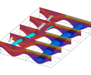
At supercritical conditions ($Re>Re_{cr}$) small amplitude perturbations result in amplification of unstable modes. We will now examine temporal evolution of a single unstable mode as it is being amplified. While amplitude of this mode remains small its growth and propagation remain governed by the linear theory. Increase of the mode's amplitude causes nonlinear interactions to become non-negligible, impeding further growth and causing the onset of the nonlinear saturation state. For the travelling wave instability, that is considered here, the growth and transition into the nonlinear saturation state bears features of the supercritical Hopf bifurcation (Yadav et al. Reference Yadav, Gepner and Szumbarski2018) with the nonlinear saturation state corresponding to the system's limit cycle. At nonlinear saturation the flow develops a number of characteristic features, not unlike those reported for the case of corrugated Poiseuille flow (Yadav et al. Reference Yadav, Gepner and Szumbarski2017). In the nonlinear solution a spanwise, periodic velocity component appears and causes the meandering-like motion of the velocity tube positioned in the diverging sections of the channel accompanied by formation of pairs of counter-rotating vortices. Both the meandering of the velocity tube as well as the vortex pairs travel through the domain at the same rate.

Here we discuss the transition to and character of the nonlinear saturation states using four characteristic cases outlined in table 1 and designated $CP_{1-4}$. Each case is considered at supercritical conditions, and of special interest to us are relations of amplification and propagation rates, characterized by components of the complex amplification rate $\sigma$, throughout the stage of exponential growth as well as times to saturation $T_s$ and periods of resulting limit cycles past the nonlinear saturation $T$ (to be compared with the period of the unstable mode $2{\rm \pi} /\sigma _r$). For each of the considered cases computational boxes span two corrugation sections in the spanwise direction and correspond to respective critical perturbation wavelengths in the streamwise direction. Consequently, computational dimensions are $(L_x,L_z)=(2\lambda _\alpha, \lambda _{\beta _{cr}})$ with spanwise and streamwise periodicity assumption maintained. For cases $CP_{1}$ and $CP_{3,4}$ the applied Reynolds number range from $110\,\%$ to $120\,\%$ of respective critical values and $CP_2$ is considered at marginally supercritical conditions of approximately $101\,\%$ of the critical Reynolds number and very close to conditions determined in § 4 as the point where the unstable mode changes direction at the lowest value of the Reynolds number, i.e. for $A\approx A^{*}$. Case $CP_1$ corresponds to zero-mean base flow at $A=0.705$ and $(Re, \beta )=(150, 0.364)$ with the unstable mode travelling in the negative $z$-direction with phase speed $v_p\approx 1.8\times 10^{-1}$ and period of the resulting limit cycle $T$ close to the period of the unstable mode resulting from the linear approximation. Cases $CP_2$ and $CP_3$ are particularly interesting and correspond to conditions that lie close to the $v_p\to 0$ line, depicted in figure 12, and feature propagation speeds of the unstable modes that are very small but with propagation in the negative $z$-direction. Case $CP_2$ is marginally critical at $(Re, \beta )=(300, 0.292)$ and close to the intersection of $Re_{cr}(A)$ and $v_p\to 0$ curves depicted in figure 12, i.e. around $A^{*}_{cr}\approx 0.462$. Consequently, this case features low phase speed of $v_p\approx 2.3\times 10^{-4}$ but also the amplification rate is moderate and small perturbation requires a long time to saturate with the resulting nonlinear state featuring a low amplitude secondary flow. Contrary, $CP_3$ at $(Re, \beta )=(340, 0.281)$ corresponds to moderate, supercritical conditions with a relatively large amplification rate and phase speed as low as $v_p\approx 10^{-5}$. For cases $CP_{2,3}$ the amplification process, starting from small, random perturbations and up to the onset of nonlinear interactions, is illustrated in the accompanying supplementary movies. At this point we note, that in the $CP_2$ case, throughout the amplification stage slowly moving structures are present. This corresponds to the small, but finite phase speed of the unstable wave travelling through the domain while it is being amplified. In the $CP_3$ case the amplification stage is much shorter and the phase speed of the least stable perturbation is much lower. Consequently, developing structures remain virtually immobile throughout the amplification stage. However, once nonlinear interactions become large enough to sufficiently change the mean flow, secondary flows begin to move and the flow settles onto a periodic cycle with a period of around $10^{4}$ advective time units, much shorter than predicted by the linear theory and apparently unrelated to the linear stability result. This discrepancy in the period of the nonlinear limit cycle past saturation with the period predicted by the linear theory result ($2{\rm \pi} /\sigma _r$) is common for both $CP_{2}$ and $CP_3$, but does not seem to be present for cases where phase velocity is higher, i.e. $CP_{1,4}$ and $P_1$. Finally, $CP_4$ at $A\approx 0.42$ and $(Re, \beta )=(460, 0.274)$ corresponds to conditions where propagation of the unstable wave reverses towards positive $z$-direction with phase speed $v_p\approx 1.6\times 10^{-2}$. For comparison, table 1 contains critical and stability properties at supercritical conditions (around $155\,\%$ of the respective $Re_{cr}$) for the travelling wave instability for the case of pure Poiseuille flow (Couette component turned off) through the considered geometry, designated as $P_1$ (compare with figure 9). We note, that amplification rate is much larger for the $P_1$ case than for the $CP_{1-4}$ ($10\unicode{x2013}10^{3}$ times larger) and that at the same time phase speed of the perturbation is around $10\unicode{x2013}10^{5}$ times that reported for $CP_{1\unicode{x2013}4}$ cases.

Table 1. Characterization of the selected cases: pressure ratio, critical and applied conditions, complex amplification $\sigma$, oscillation period past saturation $T$ and time to saturation $T_s$, phase speed and propagation direction of the perturbation for the cases selected for the study of saturation states. Cases are: Couette–Poiseuille ($CP$); Poiseuille only forcing ($P$).

Each of the considered cases is started using an undisturbed, stationary flow as the initial condition and a body force in the form of a low variance Gaussian (${Var}=10^{-5}$) noise is applied over the initial five advective time units of the simulation to excite the unstable mode. We note that the resulting initial flow state satisfies (2.2) and due to the character of the forcing a number of modes are initially energized, but only the unstable one is expected to be amplified with the rest initially attenuated, but possibly excited via nonlinear interactions after sufficiently long amplification time. Evolution of the flow is monitored using variation of the three-dimensional perturbation energy in time, defined as

(5.1)\begin{equation} E_{3D}=\frac{1}{2\varOmega}\sum_{k=1}^{k=M} \int_\varOmega \boldsymbol{u}_{{-}k}\,{\cdot}\,\boldsymbol{u}_k\,{\rm d}\varOmega, \end{equation}

with $\boldsymbol {u}_k(x,y)$ representing the $k$th amplitude of the Fourier expansion (2.8) and representing deviation from instantaneous spatial velocity average. Variation of $E_{3D}$ in time is shown in figure 13. For each case initial perturbation results in a brief, transient amplification–attenuation phase ($t\approx 100$ – see the left-hand subpanel of figure 13) followed by a prolonged stage of exponential growth (not shown), throughout which perturbation amplification is dictated by the linear mechanism. Depending on the case, exponential growth lasts in-between $10^{3}\unicode{x2013}10^{4}$ for $CP_{1,3\unicode{x2013}4}$ and up to around $10^{5}$ advective time units in the $CP_2$ case, depending on the perturbation amplification rate. Eventually nonlinear interactions impede further growth and lead the flow to the nonlinear saturation state. Using $E_{3D}$ we define saturation time $T_s$ such that $E_{3D}(t=T_s)=0.99 E_{3D}(t=T_s+1000)$, i.e. past $T_s$ perturbation energy does not change significantly with time (we tested different thresholds and time shifts, and up to reasonable values, $T_s$ does not vary much). The right-hand subpanel of figure 13 shows variation of the $E_{3D}$ around the respective saturation time $T_s$, (different for each case – see table 1).

Figure 13. Variation of the perturbation $E_{3D}$ (5.1) energy throughout saturation process for selected cases. In each case the flow is initially perturbed with an impulse of low variance Gaussian body forcing (${\textit {Var}}=10^{-5}$ over five time units) and left to develop into nonlinear saturation. Initial, transient stage ($t<250$) is shown in the left-hand subpanel, and variation around saturation time $T_s\pm 1000$ ($T_s$ is different for each case – see table 1) in the right-hand subpanel.

Past saturation time $T_s$ energy of the perturbation changes little and flow topology (shown in figures 14, 15a,b and 16) remains simple, limited to the passing of, possibly decelerated or reversed, periodic secondary flows through the domain. Due to the changes in the frequency, growth rate and phase speed of the unstable mode, distance travelled by the amplified perturbation changes significantly. Considering that the size of the prospective test domain needs to be proportional to the product of $v_p$ and $T_s$, we note that this value is decreased from around $830$ units in the case of pure Poiseuille flow ($P_1$) to $430$ for $CP_1$, $240$ for $CP_4$, $21$ for $CP_2$, and below $0.1$ for $CP_3$.

Figure 14. Snapshot of the non-stationary flow topology past the nonlinear saturation time $T_s$. Flow conditions correspond to zero-mean base flow at $A=0.705$ (case $CP_1$) and supercritical Reynolds number $Re=150$ ($Re_{cr}=124$). Length of the computational box corresponds to streamwise wavenumber $\beta =0.364$ ($\beta _{cr}=0.364$) and spans two corrugation sections in the spanwise direction. Slices on the right-hand side (left-hand side) depict streamwise velocity $w$ (streamwise vorticity $\omega _z$) contours. Stream tube (travelling vortex pair) is (are) shown in the right-hand (left-hand) part of the figure using isosurfaces of velocity (second invariant $Q$ of the velocity gradient tensor, coloured according to the positive or negative value of streamwise vorticity $\omega _z$) taken at $w=-0.4$ ($Q=3.5\times 10^{-3}$). Direction of the flow at the flat, top and next to the bottom walls, as well as instantaneous rotation of vortices and direction of the unstable wave propagation are marked using arrows. Phase speed of the unstable wave mode is $v_p=0.179$, with propagation direction aligned with applied pressure (negative $z$-direction).

Figure 15. Flow topology snapshots past saturation time $T_s$. Conditions chosen around $A^{*}$ where the direction of the wave changes ($CP_{2,3}$). Respective cases correspond to $A=0.462$, $Re=300$ and $\beta =0.292$ – case $CP_2$ – $(Re_{cr}=296$, $\beta _{cr}=0.292)$ in (a) and $A=0.455$, $Re=340$ and $\beta =0.281$ – case $CP_3$ – ($Re_{cr}=313$, $\beta _{cr}=0.281$) in (b). For both cases wave propagation is in negative $z$-direction. Slices same as in figure 14, streamwise velocity isosurfaces at $w=-0.2$ in (a,b), $Q=1.5\times 10^{-4}$ in (a) and $Q=5\times 10^{-4}$ in (b).

Figure 16. Flow topology snapshot past saturation time $T_s$. Conditions are $A=0.42$, $Re=460$ and $\beta =0.27$ (case $CP_4$, $Re_{cr}=412$, $\beta _{cr}=0.274$) with the unstable wave changing direction and propagating against applied pressure (positive $z$-direction). Slices same as in figure 14, streamwise velocity isosurfaces at $w=-0.2$ and $Q=4\times 10^{-4}$.

At nonlinear saturation the flow develops a three-dimensional form with a number of distinctive features. Figures 14 (case $CP_1$), 15(a,b) ($CP_2$ and $CP_3$) and 16 ($CP_4$) illustrate snapshots of flow topologies past nonlinear saturation time $T_s$ for each of the considered cases. One of the distinctive changes compared with the stationary solution is onset of the meandering-like motion of the streamwise velocity tubes. This is illustrated to the right-hand side in the figures by means of constant streamwise velocity surfaces (taken at $w=-0.4$ in figure 14 and $w=-0.2$ in the remaining figures and velocity-coloured slices). Onset of spanwise motions is accompanied by formation of travelling vortices, illustrated by means of isosurfaces of the second invariant $Q$ of the velocity gradient tensor, coloured by positive/negative streamwise vorticity $\omega _z$ and supplemented by arrows to indicate instantaneous rotation direction. Qualitatively, flow solutions remain similar with the exception of the marginally supercritical $CP_2$ case, which features secondary structures of very low magnitude.

In the case of corrugated channel flow with only the Poiseuille forcing applied (Yadav et al. Reference Yadav, Gepner and Szumbarski2017, Reference Yadav, Gepner and Szumbarski2021) flow features formed in consequence of nonlinear saturation propagate downstream, along the direction that the applied pressure acts. In the case of the $CP$ configuration, considered here, propagation direction might change as the Poiseuille component is decreased. Features formed as a result of nonlinear saturation of cases $CP_{1\unicode{x2013}3}$ propagate in the negative $z$-direction, marked in the figures using arrows. Case $CP_4$ corresponds to conditions where the unstable mode, and consequently three-dimensional features of the saturated flow propagates against the pressure, i.e. the positive $z$-direction.

We now focus on $CP_2$ and especially $CP_3$ cases, which we consider to be especially interesting since for those cases propagation speed of the unstable wave decreases substantially. The amplification process, starting with the initial random perturbation and past the nonlinear saturation, captured for those cases is illustrated in the accompanying supplementary movies. In the case of $CP_2$, due to the low value of the Reynolds number, amplification rate remains small, leading to a long time that is required for the nonlinear saturation to take place and allowing for the observation of the amplification phase for around $2\times 10^{5}$ advective time units. It is interesting to point out that, while formally the unstable mode remains a travelling wave and instability itself, a convective one, the time that it takes for the wave to pass through the computational domain, i.e. travel a single perturbation wavelength, is around $6.8\times 10^{4}$ time units. At the same time nonlinear effects, such as noticeable bending of the velocity tube and onset of vortex pairs, while small in amplitude due to marginal supercriticality of the case, become noticeable already around $9\times 10^{4}$ time units (the wave travels less than $1.5$ perturbation wavelengths) and throughout the entire process shown in the movie the wave travels a distance of roughly three times the length of the computational box. On the other hand, very low phase speed obtained for the unstable mode in the $CP_3$ case results in virtually no movement of the unstable mode during amplification (travelled distance is below $0.1$ length units). Consequently, throughout the amplification stage the unstable mode may be considered stationary, with resulting secondary flow structures developing both upstream and downstream.

Figure 17 illustrates this by depicting changes to the flow field at selected time instances close to the saturation time $T_s$ taken every $200$ time units. Immobility of the developing secondary flow structure is illustrated by the streamwise velocity component isosurface at $w=0.2$, which shows a developed but motionless meandering pattern formed in the diverging section of the channel. At the same time, spatial growth of the immobilized secondary flow is illustrated with isosurfaces of the second velocity gradient tensor invariant $Q$, showing spatial spread of flow regions where features of the secondary flow develop. It should be noted that spatial growth runs both in the positive as well as negative $z$-direction and developing structures are not advected by the bulk of the flow indicating that when a single, infinitely long, unstable mode is concerned, at least prior to saturation, its growth can be localized. Finally, we note that past the saturation time, possibly due to the changes to the mean flow by the nonlinear mechanism, developed secondary flow structures begin moving in the direction pointed by applied pressure and the flow settles onto a periodic cycle solution.

Figure 17. Isosurfaces of the streamwise velocity component at $w=0.2$ (grey) and second invariant $Q$ of the velocity gradient tensor at $Q=4\times 10^{-4}$ at times close to the saturation time $T_s$ for the $CP_3$ case at $t=7.6\times 10^{3}$ (a), $t=7.8\times 10^{3}$ (b) and $t=8\times 10^{3}$ (c) illustrating both upstream and downstream propagation of the secondary flow structure.

6. Extension to spatial evolution of a packet of waves

Results presented in §§ 4 and 5 stem from the application of temporal stability analysis and are limited to the considerations of a single, infinitely long, monochromatic perturbation and its temporal evolution. We will now illustrate evolution of a number of superimposed waves (a wave packet) that result from the application of a localised pulse of body forcing applied at the beginning of a simulation. For this we will consider the $CP_4$ configuration, extended to the range of unstable wave numbers (see table 1 for the details on applied flow conditions) under linear assumptions, and refer to $CP_3$ for comparison. For the sake of this illustration computational box now extends to $L_z=1024$ (approximately $45$ wavelengths of the unstable perturbation characterized in table 1). Fourier expansion (2.8) is maintained, resulting in a periodic computational box with $17$ out of $M=144$ modes representing unstable waves (see figure 18 and also discussion below). The applied initial pulse has a form of body forcing. It is applied to all velocity components and is spatially limited to streamwise positions distanced $8$ to $12$ units from the box's boundary, to ensure all unstable waves are perturbed. Additionally, an applied pulse is modulated in time as $\sin (\sigma _r t)$ with $\sigma _r$ the same as given in table 1 for the $CP_4$ case and is applied over a single period, i.e. the pulse lasts around $1430$ time units.

Figure 18. Variation of the complex amplification rate $\sigma$ in (a) and group velocity $v_g={\partial \sigma _r}/{\partial \beta }$ in (b) with the wavenumber $\beta$ at conditions corresponding to the $CP_3$ (dashed lines) and $CP_4$ (solid lines) configurations. Markers on the horizontal line correspond to wavenumbers of unstable modes amplified to form the wave packet illustrated in figure 19.

First, we compare temporal stability results obtained for $CP_3$ and $CP_4$. Figure 18(a,b) shows variation of the temporal growth rate $\sigma _i$, frequency $\sigma _r$ and of the group velocity $v_g={\partial \sigma _r}/{\partial \beta }$ as functions of the wavenumber $\beta$ in solid (dashed) lines for $CP_4$ ($CP_3$). We note that, while the range of unstable wavenumbers is similar, the frequency for the case $CP_3$ and consequently also phase velocity, decreases and changes sign within the range of those unstable wavenumbers. This means that some of the unstable waves propagate in the positive, while other in the negative direction. In fact, it is the $CP_3$ case that has been considered in § 5 as it allows for a normal mode with minimum phase velocity and a standing wave solution, when a single wave with wavenumber $\beta =0.281$ is considered. Contrary, for the $CP_4$ case the frequency is positive for the entire range of unstable wavenumbers, meaning that phase velocity of all unstable waves is directed in the positive direction, including the one selected for the nonlinear analysis in § 5 (see also figure 16). Variation of the frequency $\sigma _r$ with the wavenumber means that unstable waves are dispersive, propagate at different phase velocities and that a group of waves around a selected wavenumber $\beta _0$ will travel at a given group velocity $v_g = ({\partial \sigma _r}/{\partial \beta })(\beta _0)$. For both cases variation of group velocity is shown in figure 18(b). At this moment we note that group velocity for the pure Poiseuille forcing (no Couette component) over the range of unstable wavenumbers is in the range of approximately $v_g\in (-0.8,-0.9)$ (depending on the wavenumber $\beta$ and Reynolds number) and in the case of CP configuration at $A=1$ group velocity magnitude decreases to $v_g\in (-0.47,-0.48)$ while for the $CP_4$ it changes from $v_g\approx -0.017$ to $v_g\approx -0.029$ over the range of unstable wavenumbers. For all unstable waves the group velocity is negative, meaning that a wave packet resulting from excitation of a narrow band of waves will travel in the negative direction (Poiseuille direction using current parametrization). It is interesting to point out, that for large enough $A$ both group and phase velocity are directed in the same direction as the applied pressure (negative), but as $A$ is decreased some of the unstable waves redirect and move opposite to the group velocity, meaning that certain waves (see figure 18) propagate in the positive direction, while the packet as a whole moves in the direction of pressure, i.e. in the negative one.

Finally, figure 19 shows variation of the spanwise velocity component $u$ taken at a line passing through the computational domain at the center of the converging section, i.e. it extends from $(x,y,z)=({\rm \pi},0,0)$ to $({\rm \pi},0,L_z)$ and illustrates propagation of a wave packet that has formed as a result of the initial, localized forcing pulse. Note that since the packet travels in the negative direction, the horizontal axis has been inverted for the sake of presentation. While in the short time transient effects might be present, it is expected that only the exponential growth is observed for longer times. In figure 19(a) three distinct states, captured, respectively, at $t=3\times 10^{3}$ (dotted line), $t=10^{4}$ (dashed line) and at $t=2\times 10^{4}$ (thin solid) are shown. Comparing the change of position of the largest peak as well as its increase in amplitude the spatial growth rate evaluates to approximately $2.9\times 10^{-4}$, while group velocity of the wave packet evaluates to $v_g\approx -0.028$. We also note that the distance that the wave packet has moved during $2\times 10^{4}$ time units is approximately $500$ unit lengths or $22$ perturbation lengths considered in table 1 for the $CP_4$ case. Figure 19(b) shows the front and rear of the wave packet at $t=10^{4}$ (solid line) and after an additional $300$ time units (dashed line) and illustrates the fact that phase velocity of unstable waves points opposite than the group velocity. This results in the wave appearing as moving in the opposite direction than the wave packet moves as a whole. It is worth noting that while the wave packet, moving at a group velocity propagates faster than a single unstable mode, moving at the phase velocity does, as indicated in § 5, the reduction in the group velocity, compared with the pure Poiseuille configuration is substantial and consequently it is expected that distances required for nonlinear effects to become noticeable should decrease significantly.

Figure 19. Spanwise velocity component $u$ during linear evolution of a wave packet initiated by a localized pulse taken at a line extending from $(x,y,z)=({\rm \pi},0,0)$ to ${\rm \pi},0,L_z$. In (a) three time snapshots at $t=3\times 10^{3}$ (dotted), $t=10^{4}$ (dashed) and $t=2\times 10^{4}$ (solid). In (b) the front and rear of the wave packet at $t=10^{4}$ (dashed) and after additional $300$ time units (solid).