


1 Introduction
Over the past decades, analyses of creeping motion flows have been treated by either the Stokes equations or the Navier–Stokes equations with very low Reynolds number. When the influence of the fluid inertia term of
 $\unicode[STIX]{x1D70C}(\boldsymbol{v}\boldsymbol{\cdot }\unicode[STIX]{x1D735}\boldsymbol{v})$
is totally negligible, then the nonlinear Navier–Stokes equations are simplified to the linear Stokes equations. For example, analyses of small-scale particle dynamics, locomotion of microorganisms, the flow of red cells in the blood, Brownian motion, microfluidics and some geo-fluid dynamics, etc., belong to flow regime of the Navier–Stokes equations with very small Reynolds number. Unsteady flow past a sphere at a low Reynolds number has been addressed by Bentwich & Miloh (Reference Bentwich and Miloh1978), Sano (Reference Sano1981) and others. The study of the effects of both the inertia term of
$\unicode[STIX]{x1D70C}(\boldsymbol{v}\boldsymbol{\cdot }\unicode[STIX]{x1D735}\boldsymbol{v})$
is totally negligible, then the nonlinear Navier–Stokes equations are simplified to the linear Stokes equations. For example, analyses of small-scale particle dynamics, locomotion of microorganisms, the flow of red cells in the blood, Brownian motion, microfluidics and some geo-fluid dynamics, etc., belong to flow regime of the Navier–Stokes equations with very small Reynolds number. Unsteady flow past a sphere at a low Reynolds number has been addressed by Bentwich & Miloh (Reference Bentwich and Miloh1978), Sano (Reference Sano1981) and others. The study of the effects of both the inertia term of
 $\unicode[STIX]{x1D70C}(\boldsymbol{v}\boldsymbol{\cdot }\unicode[STIX]{x1D735}\boldsymbol{v})$
and the inertia term of
$\unicode[STIX]{x1D70C}(\boldsymbol{v}\boldsymbol{\cdot }\unicode[STIX]{x1D735}\boldsymbol{v})$
and the inertia term of
 $\unicode[STIX]{x1D70C}(\unicode[STIX]{x2202}_{t}\boldsymbol{v})$
on the fluid dynamics and capturing the deviation from the unsteady and steady Stokes equations remains open. In addition, some unsteady problems are usually considered to be a sequence of steady-state problems (a series of ‘snapshots’ of the flow) (Kim & Karrila Reference Kim and Karrila1991). This quasi-steady approach was applied successfully to capture the characteristics of motion of particles (Jeffery Reference Jeffery1922; Burgers Reference Burgers1938; Happel & Brenner Reference Happel and Brenner1965; Batchelor Reference Batchelor1970; Cox Reference Cox1970; Chwang & Wu Reference Chwang and Wu1975; Pozrikidis Reference Pozrikidis1989, Reference Pozrikidis1992). However, it is noted that no actual flows can occur without considering the effects of some fluid inertia in all real systems. For illustration, a non-negligible effect of the small inertia term of
$\unicode[STIX]{x1D70C}(\unicode[STIX]{x2202}_{t}\boldsymbol{v})$
on the fluid dynamics and capturing the deviation from the unsteady and steady Stokes equations remains open. In addition, some unsteady problems are usually considered to be a sequence of steady-state problems (a series of ‘snapshots’ of the flow) (Kim & Karrila Reference Kim and Karrila1991). This quasi-steady approach was applied successfully to capture the characteristics of motion of particles (Jeffery Reference Jeffery1922; Burgers Reference Burgers1938; Happel & Brenner Reference Happel and Brenner1965; Batchelor Reference Batchelor1970; Cox Reference Cox1970; Chwang & Wu Reference Chwang and Wu1975; Pozrikidis Reference Pozrikidis1989, Reference Pozrikidis1992). However, it is noted that no actual flows can occur without considering the effects of some fluid inertia in all real systems. For illustration, a non-negligible effect of the small inertia term of
 $\unicode[STIX]{x1D70C}(\boldsymbol{v}\boldsymbol{\cdot }\unicode[STIX]{x1D735}\boldsymbol{v})$
causes an interesting lift force (Segre & Silberberg Reference Segre and Silberberg1962; Bretherton Reference Bretherton1962; Saffman Reference Saffman1965). Another interesting example is that, by considering the influence of the inertia term of
$\unicode[STIX]{x1D70C}(\boldsymbol{v}\boldsymbol{\cdot }\unicode[STIX]{x1D735}\boldsymbol{v})$
causes an interesting lift force (Segre & Silberberg Reference Segre and Silberberg1962; Bretherton Reference Bretherton1962; Saffman Reference Saffman1965). Another interesting example is that, by considering the influence of the inertia term of
 $\unicode[STIX]{x1D70C}(\unicode[STIX]{x2202}_{t}\boldsymbol{v})$
, particles in some inter-particle or wall–particle cases have completely changed the motion characteristics of flow dynamics (Feng & Joseph Reference Feng and Joseph1995). Recently, only subjects involving the effects of the inertia term of
$\unicode[STIX]{x1D70C}(\unicode[STIX]{x2202}_{t}\boldsymbol{v})$
, particles in some inter-particle or wall–particle cases have completely changed the motion characteristics of flow dynamics (Feng & Joseph Reference Feng and Joseph1995). Recently, only subjects involving the effects of the inertia term of
 $\unicode[STIX]{x1D70C}(\unicode[STIX]{x2202}_{t}\boldsymbol{v})$
for the motion of a sphere (or slender body) or particles freely suspended in a viscous fluid have received considerable attention. The problems not only formed one of the fundamental phenomena of fluid motions, but they also arose in situations such as problems on Brownian motion (Kheifets et al.
Reference Kheifets, Simha, Melin, Li and Raizen2014; Mo et al.
Reference Mo, Simha, Kheifets and Raizen2015), the calibration of optical tweezers (Grimm, Franosch & Jeney Reference Grimm, Franosch and Jeney2012) and the dynamics of microelectromechanical systems (Clarke et al.
Reference Clarke, Jensen, Billingham and Williams2006).
$\unicode[STIX]{x1D70C}(\unicode[STIX]{x2202}_{t}\boldsymbol{v})$
for the motion of a sphere (or slender body) or particles freely suspended in a viscous fluid have received considerable attention. The problems not only formed one of the fundamental phenomena of fluid motions, but they also arose in situations such as problems on Brownian motion (Kheifets et al.
Reference Kheifets, Simha, Melin, Li and Raizen2014; Mo et al.
Reference Mo, Simha, Kheifets and Raizen2015), the calibration of optical tweezers (Grimm, Franosch & Jeney Reference Grimm, Franosch and Jeney2012) and the dynamics of microelectromechanical systems (Clarke et al.
Reference Clarke, Jensen, Billingham and Williams2006).
For the theoretical study of transient linear flows, Stokes (Reference Stokes1851) was the first to make contributions for particle dynamics in a quiescent fluid. His solution of the hydrodynamic force included the frequency of oscillation, but it only corresponded to an oscillating sphere. Basset (Reference Basset1888) extended his works and used Fourier inversion to obtain the well-known hydrodynamic force on a sphere released from rest, with the solution given by
 $$\begin{eqnarray}\displaystyle F=-6\unicode[STIX]{x03C0}\unicode[STIX]{x1D707}aU(t)-\frac{2}{3}\unicode[STIX]{x03C0}a^{3}\unicode[STIX]{x1D70C}\frac{\text{d}U}{\text{d}t}-6\unicode[STIX]{x03C0}\unicode[STIX]{x1D70C}a^{2}\sqrt{\frac{\unicode[STIX]{x1D708}}{\unicode[STIX]{x03C0}}}\int _{0}^{t}\frac{\text{d}U}{\text{d}\unicode[STIX]{x1D70F}}\frac{1}{\sqrt{t-\unicode[STIX]{x1D70F}}}\,\text{d}\unicode[STIX]{x1D70F}, & & \displaystyle\end{eqnarray}$$
where
 $U(t)$
and
$U(t)$
and
 $a$
are the velocity and the radius of the sphere, respectively;
$a$
are the velocity and the radius of the sphere, respectively;
 $\unicode[STIX]{x1D70C}$
and
$\unicode[STIX]{x1D70C}$
and
 $\unicode[STIX]{x1D707}$
are the density and dynamic viscosity of the fluid, respectively, and
$\unicode[STIX]{x1D707}$
are the density and dynamic viscosity of the fluid, respectively, and
 $\unicode[STIX]{x1D708}=\unicode[STIX]{x1D707}/\unicode[STIX]{x1D70C}$
is the kinematic viscosity of the fluid. The first term on the right-hand side of (1.1) is the well-known quasi-steady Stokes drag, the second term on the right-hand side is the added mass term. The third term on the right-hand side is the Basset memory force, which depends on past history of the particle motion, such as the rate change of the sphere velocity.
$\unicode[STIX]{x1D708}=\unicode[STIX]{x1D707}/\unicode[STIX]{x1D70C}$
is the kinematic viscosity of the fluid. The first term on the right-hand side of (1.1) is the well-known quasi-steady Stokes drag, the second term on the right-hand side is the added mass term. The third term on the right-hand side is the Basset memory force, which depends on past history of the particle motion, such as the rate change of the sphere velocity.
In addition, another classical solution for transient motion is that of a rotating sphere in a quiescent fluid. This problem was solved analytically by some researchers (e.g. Landau & Lifshitz Reference Landau and Lifshitz1959; Feuillebois & Lasek Reference Feuillebois and Lasek1978). The torque on a rotating sphere from rest with an arbitrary differentiable angular velocity
 $\unicode[STIX]{x1D74E}(t)$
is given by
$\unicode[STIX]{x1D74E}(t)$
is given by
 $$\begin{eqnarray}\displaystyle \boldsymbol{C}(t) & = & \displaystyle -8\unicode[STIX]{x03C0}\unicode[STIX]{x1D707}a^{3}\left[\unicode[STIX]{x1D74E}(t)+\frac{1}{3}\frac{a}{\sqrt{\unicode[STIX]{x03C0}\unicode[STIX]{x1D708}}}\int _{0}^{t}\frac{\text{d}\unicode[STIX]{x1D74E}(\unicode[STIX]{x1D70F})}{\text{d}\unicode[STIX]{x1D70F}}\frac{1}{\sqrt{t-\unicode[STIX]{x1D70F}}}\,\text{d}\unicode[STIX]{x1D70F}\right.\nonumber\\ \displaystyle & & \displaystyle \left.-\,\frac{1}{3}\int _{0}^{t}\frac{\text{d}\unicode[STIX]{x1D74E}(\unicode[STIX]{x1D70F})}{\text{d}\unicode[STIX]{x1D70F}}\exp \left(\frac{\unicode[STIX]{x1D708}(t-\unicode[STIX]{x1D70F})}{a^{2}}\right)\text{erfc}\left(\frac{\sqrt{\unicode[STIX]{x1D708}(t-\unicode[STIX]{x1D70F})}}{a}\right)\,\text{d}\unicode[STIX]{x1D70F}\right],\end{eqnarray}$$
where
 $\exp (x)$
is the exponential function,
$\exp (x)$
is the exponential function,
 $\text{erfc}(x)=1-\text{erf}(x)$
is the complementary error function and
$\text{erfc}(x)=1-\text{erf}(x)$
is the complementary error function and
 $\text{erf}(x)$
is the error function. The first term on the right-hand side of (1.2) is the quasi-steady torque and the other two terms on the right-hand side involve memory kernels. In particular, there is no ‘added torque of inertia’ term in the rotary motion. The second term on the right-hand side of (1.2) is of the same decaying order as the Basset integral in (1.1). In addition, the memory kernels function
$\text{erf}(x)$
is the error function. The first term on the right-hand side of (1.2) is the quasi-steady torque and the other two terms on the right-hand side involve memory kernels. In particular, there is no ‘added torque of inertia’ term in the rotary motion. The second term on the right-hand side of (1.2) is of the same decaying order as the Basset integral in (1.1). In addition, the memory kernels function
 $\exp (\unicode[STIX]{x1D708}t/a^{2})\text{erfc}(\sqrt{\unicode[STIX]{x1D708}t}/a)\approx a/\sqrt{\unicode[STIX]{x03C0}\unicode[STIX]{x1D708}t}$
at very short time
$\exp (\unicode[STIX]{x1D708}t/a^{2})\text{erfc}(\sqrt{\unicode[STIX]{x1D708}t}/a)\approx a/\sqrt{\unicode[STIX]{x03C0}\unicode[STIX]{x1D708}t}$
at very short time
 $t\ll a^{2}/\unicode[STIX]{x1D708}$
. It is also noted that the third term on the right-hand side of (1.2) has a negative sign. Therefore, the two terms involving the memory kernels in (1.2) decay much faster than the Basset memory force as the motions tend to become steady (see Feuillebois & Lasek Reference Feuillebois and Lasek1978, p. 442).
$t\ll a^{2}/\unicode[STIX]{x1D708}$
. It is also noted that the third term on the right-hand side of (1.2) has a negative sign. Therefore, the two terms involving the memory kernels in (1.2) decay much faster than the Basset memory force as the motions tend to become steady (see Feuillebois & Lasek Reference Feuillebois and Lasek1978, p. 442).
The other important result of the transient solutions is the hydrodynamic force on a slightly deformed translating spheroid. By applying Fourier transforms to the governing unsteady Stokes equations and using the dimensionless variables
 $U^{\ast }=U/V$
,
$U^{\ast }=U/V$
,
 $\boldsymbol{x}^{\ast }=\boldsymbol{x}/L$
,
$\boldsymbol{x}^{\ast }=\boldsymbol{x}/L$
,
 $t^{\ast }=t/T$
,
$t^{\ast }=t/T$
,
 $p^{\ast }=pL/\unicode[STIX]{x1D707}V$
, Lawrence & Weinbaum (Reference Lawrence and Weinbaum1986) were able to obtain the dimensionless force on the spheroid (after dropping the stars) as
$p^{\ast }=pL/\unicode[STIX]{x1D707}V$
, Lawrence & Weinbaum (Reference Lawrence and Weinbaum1986) were able to obtain the dimensionless force on the spheroid (after dropping the stars) as
 $$\begin{eqnarray}\displaystyle F & = & \displaystyle -6\unicode[STIX]{x03C0}\left(1+\frac{4}{5}\unicode[STIX]{x1D700}+\frac{2}{175}\unicode[STIX]{x1D700}^{2}\right)U(t)-\frac{2}{3}\unicode[STIX]{x03C0}\left(1+\frac{16}{5}\unicode[STIX]{x1D700}+\frac{604}{175}\unicode[STIX]{x1D700}^{2}\right)\frac{\text{d}U}{\text{d}t}\nonumber\\ \displaystyle & & \displaystyle -\,6\sqrt{\unicode[STIX]{x03C0}}\left(1+\frac{8}{5}\unicode[STIX]{x1D700}+\frac{116}{175}\unicode[STIX]{x1D700}^{2}\right)\int _{0}^{t}\frac{\text{d}U}{\text{d}\unicode[STIX]{x1D70F}}\frac{1}{\sqrt{t-\unicode[STIX]{x1D70F}}}\,\text{d}\unicode[STIX]{x1D70F}\nonumber\\ \displaystyle & & \displaystyle -\,\frac{8}{175}\left(\frac{\unicode[STIX]{x03C0}}{3}\right)^{1/2}\unicode[STIX]{x1D700}^{2}\int _{0}^{t}\frac{\text{d}U}{\text{d}\unicode[STIX]{x1D70F}}G(t-\unicode[STIX]{x1D70F})\,\text{d}\unicode[STIX]{x1D70F}+O(\unicode[STIX]{x1D700}^{3})\nonumber\\ \displaystyle & & \displaystyle \text{with }G(t)=\text{Im}(\sqrt{\unicode[STIX]{x03C0}\unicode[STIX]{x1D702}}\text{e}^{\unicode[STIX]{x1D702}t}\text{erfc}(\sqrt{\unicode[STIX]{x1D702}t})),\quad \unicode[STIX]{x1D702}=(3+3\sqrt{3}\text{i})/2.\end{eqnarray}$$
A slightly deformed spheroid with semiaxes is related by
 $a=b(1+\unicode[STIX]{x1D700})$
, where
$a=b(1+\unicode[STIX]{x1D700})$
, where
 $a$
,
$a$
,
 $b$
is the semimajor and semiminor axis, respectively, and
$b$
is the semimajor and semiminor axis, respectively, and
 $\unicode[STIX]{x1D700}$
is a perturbation parameter. A new memory force that decays faster than the Basset memory force was found in the last term on the right-hand side of (1.3). Until recently there have been few analytical results available for solving unsteady Stokes flow problems (e.g. Basset Reference Basset1888; Landau & Lifshitz Reference Landau and Lifshitz1959; Feuillebois & Lasek Reference Feuillebois and Lasek1978 and Lawrence & Weinbaum Reference Lawrence and Weinbaum1986). Most of the analytical results are limited to the cases of a uniform free stream or an oscillatory motion of a sphere or spheroid. In general the flow fields are spatially inhomogeneous and undisturbed, such as linear or parabolic flows, which are more significant from practical and experimental points of view. Mazur & Bedeaux (Reference Mazur and Bedeaux1974) have derived the viscous drag on a sphere moving with an arbitrary velocity for unsteady, spatially inhomogeneous flows. Faxén’s law was then extended to transient Stokes flows. However, investigations into finding the analytical unsteady hydrodynamic force or torque remain largely unexplored at present. Maybe the possible difficulty arises when traditional analytical methods are used which employ the separation of the variables and Fourier inversion, as well as under the assumption of small-amplitude harmonic oscillation of a particle.
$\unicode[STIX]{x1D700}$
is a perturbation parameter. A new memory force that decays faster than the Basset memory force was found in the last term on the right-hand side of (1.3). Until recently there have been few analytical results available for solving unsteady Stokes flow problems (e.g. Basset Reference Basset1888; Landau & Lifshitz Reference Landau and Lifshitz1959; Feuillebois & Lasek Reference Feuillebois and Lasek1978 and Lawrence & Weinbaum Reference Lawrence and Weinbaum1986). Most of the analytical results are limited to the cases of a uniform free stream or an oscillatory motion of a sphere or spheroid. In general the flow fields are spatially inhomogeneous and undisturbed, such as linear or parabolic flows, which are more significant from practical and experimental points of view. Mazur & Bedeaux (Reference Mazur and Bedeaux1974) have derived the viscous drag on a sphere moving with an arbitrary velocity for unsteady, spatially inhomogeneous flows. Faxén’s law was then extended to transient Stokes flows. However, investigations into finding the analytical unsteady hydrodynamic force or torque remain largely unexplored at present. Maybe the possible difficulty arises when traditional analytical methods are used which employ the separation of the variables and Fourier inversion, as well as under the assumption of small-amplitude harmonic oscillation of a particle.
The main purpose of this study is to obtain the exact solutions in more general time-dependent flows instead of adopting the elections of many other available analytical techniques. The singularity method is an inverse problem approach and the main shortcomings are too general to guide the proper choice of singularities for all the systematized situations. However, this method is more direct and simpler than the conventional harmonic functions method, which is based on the choice of a suitable coordinate system and uses known classical methods to obtain exact solutions. The usage of the singularity method in the analysis of a wide variety of steady Stokes flow problems has proven to be a valuable tool and presented fruitful results (e.g. Oseen Reference Oseen1927; Burgers Reference Burgers1938; Batchelor Reference Batchelor1970; Cox Reference Cox1970; Blake Reference Blake1971; Chwang & Wu Reference Chwang and Wu1975; Lighthill Reference Lighthill1996). However, theoretical treatments using the singularity method are mostly limited to steady Stokes equations. We hope the spirit of the singularity method and time convolution integral technique will be carried out for more general transient Stokes hydrodynamics problems by following the past valuable experiences of steady Stokes flows. In recent years, an unsteady Stokeslet has been presented by a number of investigators for unsteady Stokes flow problems (e.g. Hasegawa, Onishi & Soya Reference Hasegawa, Onishi and Soya1986; Smith Reference Smith1987; Pozrikidis Reference Pozrikidis1989, Reference Pozrikidis1992; Avudainayagam & Geetha Reference Avudainayagam and Geetha1995; Chan & Chwang Reference Chan and Chwang2000; Shu & Chwang Reference Shu and Chwang2001; Guenther & Thomann Reference Guenther and Thomann2007; Hsiao & Young Reference Hsiao and Young2015). Nevertheless most works on the subject only use an unsteady Stokeslet or oscillatory singularities as a function of the frequency of oscillation
 $\unicode[STIX]{x1D74E}$
(see also Pozrikidis Reference Pozrikidis1989). A novel technique for the hydrodynamic force with the convolution quadrature method (CQM) (Lubich & Schadle Reference Lubich and Schadle2002) coupled with fundamental solutions has been presented by Hsiao & Young (Reference Hsiao and Young2014) recently.
$\unicode[STIX]{x1D74E}$
(see also Pozrikidis Reference Pozrikidis1989). A novel technique for the hydrodynamic force with the convolution quadrature method (CQM) (Lubich & Schadle Reference Lubich and Schadle2002) coupled with fundamental solutions has been presented by Hsiao & Young (Reference Hsiao and Young2014) recently.
We will extend the above results and derive higher-order time–space fundamental solutions (for example, an unsteady rotlet, an unsteady Stokeslet doublet, an unsteady stresslet, and an unsteady Stokeslet quadrupole) in § 2. The fundamental solutions in unsteady Stokes flow must be derived first. Next these time-dependent fundamental solutions obtained will be then used to express the solutions as a convolution integral in time. Finally, we will calculate solutions of the time-dependent force and torque on a sphere in a shear flow and also in a parabolic flow by using the Laplace transform technique. An attempt will be made to look for unknown solutions of new and more complicated unsteady Stokes flow problems. We will use the coupling between the time convolution integral and the superposition technique of the foregoing fundamental solutions including force singularities and potential singularities to construct the requisite flow structures. In § 3, a study of the transient flow of a sphere rotating in a viscous fluid will be carried out. This well-known solution is also solved by using different methods. It is also used to validate our analytical work by comparison to other derivations. In §§ 4–6, we will focus on exact solutions of a simple shear flow past a sphere, a sphere with free rotation in a simple shear flow and an axisymmetric parabolic flow past a sphere. These transient flow structures may be the first derived as far as unsteady Stokes flow problems are concerned. The force and torque solutions of unsteady or steady Stokes flow problems may serve as challenging benchmarks for numerical modellers to verify the accuracy of their numerical methods after obtaining their viscous and pressure forces. Section 7 contains a short concluding remark.
2 An unsteady Stokeslet and higher-order singularities
2.1 An unsteady Stokeslet
The fundamental solution of unsteady Stokes flow represents the solution due to a concentrated point force
 $\boldsymbol{f}_{ext}$
, which has a singularity at the point
$\boldsymbol{f}_{ext}$
, which has a singularity at the point
 $\boldsymbol{x}_{\mathbf{0}}$
and at time
$\boldsymbol{x}_{\mathbf{0}}$
and at time
 $t=0$
. The governing equation is
$t=0$
. The governing equation is
 $$\begin{eqnarray}\displaystyle \left.\begin{array}{@{}c@{}}\unicode[STIX]{x1D735}\boldsymbol{\cdot }\boldsymbol{u}=0,\\ \displaystyle \unicode[STIX]{x1D70C}\frac{\unicode[STIX]{x2202}\boldsymbol{u}}{\unicode[STIX]{x2202}t}=-\unicode[STIX]{x1D735}p^{S}+\unicode[STIX]{x1D707}\unicode[STIX]{x1D6FB}^{2}\boldsymbol{u}+\boldsymbol{f}_{ext}\end{array}\right\}, & & \displaystyle\end{eqnarray}$$
where
 $\boldsymbol{f}_{ext}(\boldsymbol{x},t)=\unicode[STIX]{x1D736}\unicode[STIX]{x1D6FF}(\boldsymbol{x}-\boldsymbol{x}_{\mathbf{0}})\unicode[STIX]{x1D6FF}(t)$
is the external force,
$\boldsymbol{f}_{ext}(\boldsymbol{x},t)=\unicode[STIX]{x1D736}\unicode[STIX]{x1D6FF}(\boldsymbol{x}-\boldsymbol{x}_{\mathbf{0}})\unicode[STIX]{x1D6FF}(t)$
is the external force,
 $\boldsymbol{u}=(u,v,w)$
is the fluid velocity,
$\boldsymbol{u}=(u,v,w)$
is the fluid velocity,
 $\unicode[STIX]{x1D70C}$
is the fluid density,
$\unicode[STIX]{x1D70C}$
is the fluid density,
 $p^{S}$
is the fluid pressure,
$p^{S}$
is the fluid pressure,
 $\unicode[STIX]{x1D707}$
is the dynamic viscosity of fluid,
$\unicode[STIX]{x1D707}$
is the dynamic viscosity of fluid,
 $\unicode[STIX]{x1D736}=(\unicode[STIX]{x1D6FC}_{1},\unicode[STIX]{x1D6FC}_{2},\unicode[STIX]{x1D6FC}_{3})$
is a constant vector and stands for the strength of the point force in a three-dimensional Euclidean space respectively,
$\unicode[STIX]{x1D736}=(\unicode[STIX]{x1D6FC}_{1},\unicode[STIX]{x1D6FC}_{2},\unicode[STIX]{x1D6FC}_{3})$
is a constant vector and stands for the strength of the point force in a three-dimensional Euclidean space respectively,
 $\unicode[STIX]{x1D6FF}$
is the Dirac delta function and
$\unicode[STIX]{x1D6FF}$
is the Dirac delta function and
 $\boldsymbol{x}$
is the position vector. The solution in three dimensions for the velocity field is given as
$\boldsymbol{x}$
is the position vector. The solution in three dimensions for the velocity field is given as
 $$\begin{eqnarray}\displaystyle u_{i}(\boldsymbol{x},t)=\frac{1}{4\unicode[STIX]{x03C0}\unicode[STIX]{x1D70C}}G_{ij}^{S}(\hat{\boldsymbol{x}},t)\unicode[STIX]{x1D6FC}_{j}, & & \displaystyle\end{eqnarray}$$
 $$\begin{eqnarray}\displaystyle G_{ij}^{S}(\hat{\boldsymbol{x}},t) & = & \displaystyle \frac{1}{\sqrt{\unicode[STIX]{x03C0}\unicode[STIX]{x1D708}t}}\left(\frac{r^{2}\unicode[STIX]{x1D6FF}_{ij}-\hat{x}_{i}\hat{x}_{j}}{2\unicode[STIX]{x1D708}tr^{2}}-\frac{2}{r^{2}}\unicode[STIX]{x1D6FF}_{ij}+\frac{3(r^{2}\unicode[STIX]{x1D6FF}_{ij}-\hat{x}_{i}\hat{x}_{j})}{r^{4}}\right)\exp \left(-\frac{r^{2}}{4\unicode[STIX]{x1D708}t}\right)\nonumber\\ \displaystyle & & \displaystyle -\,\frac{(r^{2}\unicode[STIX]{x1D6FF}_{ij}-3\hat{x}_{i}\hat{x}_{j})}{r^{5}}\text{erf}\left(\frac{r}{\sqrt{4\unicode[STIX]{x1D708}t}}\right).\end{eqnarray}$$
Here
 $r=|\hat{\boldsymbol{x}}|$
,
$r=|\hat{\boldsymbol{x}}|$
,
 $\hat{\boldsymbol{x}}=\boldsymbol{x}-\boldsymbol{x}_{\mathbf{0}}$
,
$\hat{\boldsymbol{x}}=\boldsymbol{x}-\boldsymbol{x}_{\mathbf{0}}$
,
 $\unicode[STIX]{x1D708}=\unicode[STIX]{x1D707}/\unicode[STIX]{x1D70C}$
is the kinematic viscosity of fluid and
$\unicode[STIX]{x1D708}=\unicode[STIX]{x1D707}/\unicode[STIX]{x1D70C}$
is the kinematic viscosity of fluid and
 $G_{ij}^{S}(\hat{\boldsymbol{x}},t)$
is a free-space Green’s function, also called a fundamental solution or an unsteady Stokeslet. The induced pressure is
$G_{ij}^{S}(\hat{\boldsymbol{x}},t)$
is a free-space Green’s function, also called a fundamental solution or an unsteady Stokeslet. The induced pressure is
 $$\begin{eqnarray}\displaystyle p^{S}(\boldsymbol{x},t)=\frac{\unicode[STIX]{x1D6FF}(t)}{4\unicode[STIX]{x03C0}}\frac{\hat{x}_{i}}{r^{3}}\unicode[STIX]{x1D6FC}_{i}. & & \displaystyle\end{eqnarray}$$
The surrounding fluid exerts a force on the control surface
 $S_{c}$
of a sphere with radius
$S_{c}$
of a sphere with radius
 $a$
centred at the point impulse
$a$
centred at the point impulse
 $\unicode[STIX]{x1D736}$
. The total forces are given by
$\unicode[STIX]{x1D736}$
. The total forces are given by
 $$\begin{eqnarray}\displaystyle \boldsymbol{f}=-\frac{\unicode[STIX]{x1D736}}{\sqrt{\unicode[STIX]{x03C0}\unicode[STIX]{x1D708}t}}\left(\frac{a^{3}}{6\unicode[STIX]{x1D708}t^{2}}\right)\exp \left(-\frac{a^{2}}{4\unicode[STIX]{x1D708}t}\right)-\frac{1}{3}\unicode[STIX]{x1D736}\unicode[STIX]{x1D6FF}(t). & & \displaystyle\end{eqnarray}$$
Furthermore, in (2.5) it is observed that the first term and the second term on the right-hand side come from viscous force and the pressure, respectively. The aforementioned formulations have been presented by Hsiao & Young (Reference Hsiao and Young2015).
2.2 An unsteady Stokes doublet
By linear differential equations, the derivatives of
 $u_{i}(\boldsymbol{x},t)$
,
$u_{i}(\boldsymbol{x},t)$
,
 $p^{S}(\boldsymbol{x},t)$
in (2.2), (2.4) are also solutions of (2.1). Therefore, we differentiate an unsteady Stokeslet with respect to
$p^{S}(\boldsymbol{x},t)$
in (2.2), (2.4) are also solutions of (2.1). Therefore, we differentiate an unsteady Stokeslet with respect to
 $\boldsymbol{x}_{\pmb{{\it 0}}}$
. This means that we take the gradient of (2.3) in the chosen direction. Hence, the induced velocity in three dimensions is
$\boldsymbol{x}_{\pmb{{\it 0}}}$
. This means that we take the gradient of (2.3) in the chosen direction. Hence, the induced velocity in three dimensions is
 $$\begin{eqnarray}\displaystyle u_{i}(\boldsymbol{x},t)=\frac{1}{4\unicode[STIX]{x03C0}\unicode[STIX]{x1D70C}}G_{ijk}^{SD}(\hat{\boldsymbol{x}},t)d_{jk}. & & \displaystyle\end{eqnarray}$$
Following Blake (Reference Blake1971) and Chwang & Wu (Reference Chwang and Wu1975),
 $G_{ijk}^{SD}(\hat{\boldsymbol{x}},t)$
is called an unsteady Stokeslet doublet and
$G_{ijk}^{SD}(\hat{\boldsymbol{x}},t)$
is called an unsteady Stokeslet doublet and
 $d_{jk}$
is the strength of singularity by a second-order tensor. Next,
$d_{jk}$
is the strength of singularity by a second-order tensor. Next,
 $G_{ijk}^{SD}(\hat{\boldsymbol{x}},t)$
is expressed in the form
$G_{ijk}^{SD}(\hat{\boldsymbol{x}},t)$
is expressed in the form
 $$\begin{eqnarray}\displaystyle G_{ijk}^{SD}(\hat{\boldsymbol{x}},t) & = & \displaystyle \frac{\unicode[STIX]{x2202}G_{ij}^{S}(\hat{\boldsymbol{x}},t)}{\unicode[STIX]{x2202}x_{0,k}}=-\frac{\unicode[STIX]{x2202}G_{ij}^{S}(\hat{\boldsymbol{x}},t)}{\unicode[STIX]{x2202}\hat{x}_{k}}\nonumber\\ \displaystyle & = & \displaystyle \frac{1}{\sqrt{\unicode[STIX]{x03C0}\unicode[STIX]{x1D708}t}}\left(\begin{array}{@{}l@{}}\displaystyle \frac{(3\hat{x}_{k}\unicode[STIX]{x1D6FF}_{ij}+3\hat{x}_{i}\unicode[STIX]{x1D6FF}_{jk}+3\hat{x}_{j}\unicode[STIX]{x1D6FF}_{ik})}{r^{4}}-\frac{15\hat{x}_{i}\hat{x}_{j}\hat{x}_{k}}{r^{6}}\\ \displaystyle +\,\frac{(\hat{x}_{k}\unicode[STIX]{x1D6FF}_{ij}+\hat{x}_{i}\unicode[STIX]{x1D6FF}_{jk}+\hat{x}_{j}\unicode[STIX]{x1D6FF}_{ik})}{2\unicode[STIX]{x1D708}tr^{2}}-\frac{5\hat{x}_{i}\hat{x}_{j}\hat{x}_{k}}{2\unicode[STIX]{x1D708}tr^{4}}\\ \displaystyle +\,\frac{\hat{x}_{k}\unicode[STIX]{x1D6FF}_{ij}}{4\unicode[STIX]{x1D708}^{2}t^{2}}-\frac{\hat{x}_{i}\hat{x}_{j}\hat{x}_{k}}{4\unicode[STIX]{x1D708}^{2}t^{2}r^{2}}\end{array}\right)\exp \left(-\frac{r^{2}}{4\unicode[STIX]{x1D708}t}\right)\nonumber\\ \displaystyle & & \displaystyle -\,\frac{(3\hat{x}_{k}\unicode[STIX]{x1D6FF}_{ij}+3\hat{x}_{i}\unicode[STIX]{x1D6FF}_{jk}+3\hat{x}_{j}\unicode[STIX]{x1D6FF}_{ik})}{r^{5}}\text{erf}\left(\frac{r}{\sqrt{4\unicode[STIX]{x1D708}t}}\right)+\frac{15\hat{x}_{i}\hat{x}_{j}\hat{x}_{k}}{r^{7}}\text{erf}\left(\frac{r}{\sqrt{4\unicode[STIX]{x1D708}t}}\right).\end{eqnarray}$$
Similarly, the induced pressure of an unsteady Stokeslet doublet is
 $$\begin{eqnarray}\displaystyle p^{SD}(\boldsymbol{x},t)=\frac{\unicode[STIX]{x2202}p^{S}(\hat{\boldsymbol{x}},t)}{\unicode[STIX]{x2202}x_{0,k}}=\frac{\unicode[STIX]{x1D6FF}(t)}{4\unicode[STIX]{x03C0}}\left(-\frac{\unicode[STIX]{x1D6FF}_{jk}}{r^{3}}+3\frac{\hat{x}_{j}\hat{x}_{k}}{r^{5}}\right)d_{jk}. & & \displaystyle\end{eqnarray}$$
Physically, an unsteady Stokeslet doublet means the induced velocity is due to a point force dipole. Now, by integrating equation (2.6) with respect to
 $t$
from 0 to
$t$
from 0 to
 $\infty$
, it is found that
$\infty$
, it is found that
 $$\begin{eqnarray}\displaystyle \int _{0}^{\infty }u_{i}(\boldsymbol{x},t)\,\text{d}t & = & \displaystyle \int _{0}^{\infty }\frac{1}{4\unicode[STIX]{x03C0}\unicode[STIX]{x1D70C}}G_{ijk}^{SD}(\hat{\boldsymbol{x}},t)d_{jk}\,\text{d}t\nonumber\\ \displaystyle & = & \displaystyle \frac{1}{8\unicode[STIX]{x03C0}\unicode[STIX]{x1D707}}\left(\frac{\hat{x}_{k}\unicode[STIX]{x1D6FF}_{ij}-\hat{x}_{i}\unicode[STIX]{x1D6FF}_{jk}-\hat{x}_{j}\unicode[STIX]{x1D6FF}_{ik}}{r^{3}}+\frac{3\hat{x}_{i}\hat{x}_{j}\hat{x}_{k}}{r^{5}}\right)d_{jk}.\end{eqnarray}$$
Equation (2.9) is in agreement with the steady Stokeslet doublet given by Blake (Reference Blake1971), Chwang & Wu (Reference Chwang and Wu1975) and Pozrikidis (Reference Pozrikidis1992).
2.3 An unsteady rotlet
We now consider an unsteady rotlet (also called a couplet in steady Stokes flow by Batchelor (Reference Batchelor1970)), which regards the fundamental solution due to a point couple which has a singularity at the point
 $\boldsymbol{x}_{\pmb{{\it 0}}}$
and at time
$\boldsymbol{x}_{\pmb{{\it 0}}}$
and at time
 $t=0$
, in a fluid otherwise at rest. The governing equation is
$t=0$
, in a fluid otherwise at rest. The governing equation is
 $$\begin{eqnarray}\displaystyle \left.\begin{array}{@{}c@{}}\unicode[STIX]{x1D735}\boldsymbol{\cdot }\boldsymbol{u}=0,\\ \displaystyle \unicode[STIX]{x1D70C}\frac{\unicode[STIX]{x2202}\boldsymbol{u}}{\unicode[STIX]{x2202}t}=-\unicode[STIX]{x1D735}p+\unicode[STIX]{x1D707}\unicode[STIX]{x1D6FB}^{2}\boldsymbol{u}+\unicode[STIX]{x1D735}\times (\unicode[STIX]{x1D734}\unicode[STIX]{x1D6FF}(\boldsymbol{x}-\boldsymbol{x}_{\pmb{{\it 0}}})\unicode[STIX]{x1D6FF}(t))\end{array}\right\}. & & \displaystyle\end{eqnarray}$$
Since we are looking for rotational flow, the pressure is assumed to be constant. On the other hand,
 $\unicode[STIX]{x1D734}$
is a constant vector, so that
$\unicode[STIX]{x1D734}$
is a constant vector, so that
 $\unicode[STIX]{x1D735}\times \unicode[STIX]{x1D734}=0$
. After using vector identities, equation (2.10) becomes
$\unicode[STIX]{x1D735}\times \unicode[STIX]{x1D734}=0$
. After using vector identities, equation (2.10) becomes
 $$\begin{eqnarray}\displaystyle \unicode[STIX]{x1D70C}\frac{\unicode[STIX]{x2202}\boldsymbol{u}}{\unicode[STIX]{x2202}t}=\unicode[STIX]{x1D707}\unicode[STIX]{x1D6FB}^{2}\boldsymbol{u}+\unicode[STIX]{x1D735}\unicode[STIX]{x1D6FF}(\hat{\boldsymbol{x}})\times \unicode[STIX]{x1D734}\unicode[STIX]{x1D6FF}(t). & & \displaystyle\end{eqnarray}$$
By taking the Laplace transform of (2.11) with respect to
 $t$
, we obtain
$t$
, we obtain
 $$\begin{eqnarray}\displaystyle \unicode[STIX]{x1D70C}s\hat{\boldsymbol{u}}(s,\boldsymbol{x})=\unicode[STIX]{x1D707}\unicode[STIX]{x1D6FB}^{2}\hat{\boldsymbol{u}}(s,\boldsymbol{x})+\unicode[STIX]{x1D735}\unicode[STIX]{x1D6FF}(\hat{\boldsymbol{x}})\times \unicode[STIX]{x1D734}. & & \displaystyle\end{eqnarray}$$
The Laplace transform of a function
 $\boldsymbol{u}(t,\boldsymbol{x})$
, defined for all real numbers
$\boldsymbol{u}(t,\boldsymbol{x})$
, defined for all real numbers
 $t\geqslant 0$
, is the function
$t\geqslant 0$
, is the function
 $\hat{\boldsymbol{u}}(s,\boldsymbol{x})$
, defined by
$\hat{\boldsymbol{u}}(s,\boldsymbol{x})$
, defined by
 $$\begin{eqnarray}\displaystyle \mathscr{L}(\boldsymbol{u}(t,\boldsymbol{x}))=\hat{\boldsymbol{u}}(s,\boldsymbol{x})=\int _{0}^{\infty }\boldsymbol{u}(t,\boldsymbol{x})\exp (-st)\,\text{d}t. & & \displaystyle\end{eqnarray}$$
Again taking the Fourier transform of (2.12) we obtain
 $$\begin{eqnarray}\displaystyle \unicode[STIX]{x1D70C}s\bar{\hat{\boldsymbol{u}}}(s,\boldsymbol{k})=-\unicode[STIX]{x1D707}(k_{x}^{2}+k_{y}^{2}+k_{z}^{2})\bar{\hat{\boldsymbol{u}}}+\frac{1}{(2\unicode[STIX]{x03C0})^{3/2}}(\text{i}k_{x}\hat{i} +\text{i}k_{y}{\hat{j}}+\text{i}k_{z}\hat{k})\text{e}^{-\text{i}\boldsymbol{k}\boldsymbol{\cdot }\boldsymbol{x}_{\mathbf{0}}}\times \unicode[STIX]{x1D734}. & & \displaystyle\end{eqnarray}$$
The Fourier transform of a function
 $\hat{\boldsymbol{u}}(s,\boldsymbol{x})$
is defined by
$\hat{\boldsymbol{u}}(s,\boldsymbol{x})$
is defined by
 $$\begin{eqnarray}\displaystyle \mathscr{F}(\hat{\boldsymbol{u}}(s,\boldsymbol{x}))=\bar{\hat{\boldsymbol{u}}}(s,\boldsymbol{k})=\frac{1}{(2\unicode[STIX]{x03C0})^{3/2}}\int _{\boldsymbol{E}^{3}}\hat{\boldsymbol{u}}(s,\boldsymbol{x})\exp (-\text{i}(\boldsymbol{k}\boldsymbol{\cdot }\boldsymbol{x}))\,\text{d}\boldsymbol{x}, & & \displaystyle\end{eqnarray}$$
where
 $\boldsymbol{E}^{3}$
denotes the three-dimensional Euclidean space and
$\boldsymbol{E}^{3}$
denotes the three-dimensional Euclidean space and
 $\boldsymbol{k}=(k_{x},k_{y},k_{z})$
is a constant vector, respectively. After a straightforward algebra manipulation, equation (2.14) now becomes
$\boldsymbol{k}=(k_{x},k_{y},k_{z})$
is a constant vector, respectively. After a straightforward algebra manipulation, equation (2.14) now becomes
 $$\begin{eqnarray}\displaystyle \bar{\hat{\boldsymbol{u}}}(s,\boldsymbol{k})=\frac{\text{i}}{(2\unicode[STIX]{x03C0})^{3/2}\unicode[STIX]{x1D70C}}\left(\frac{k_{x}}{s+\unicode[STIX]{x1D708}\Vert \boldsymbol{k}\Vert ^{2}}\hat{i} +\frac{k_{y}}{s+\unicode[STIX]{x1D708}\Vert \boldsymbol{k}\Vert ^{2}}{\hat{j}}+\frac{k_{z}}{s+\unicode[STIX]{x1D708}\Vert \boldsymbol{k}\Vert ^{2}}\hat{k}\right)\text{e}^{-\text{i}\boldsymbol{k}\boldsymbol{\cdot }\boldsymbol{x}_{\mathbf{0}}}\times \unicode[STIX]{x1D734}. & & \displaystyle\end{eqnarray}$$
Taking the Laplace and Fourier inversions of (2.16), we obtain the fundamental solution of an unsteady rotlet in the vector form
 $$\begin{eqnarray}\displaystyle \boldsymbol{u}(\boldsymbol{x},t) & = & \displaystyle \frac{1}{(2\unicode[STIX]{x03C0})^{3/2}\unicode[STIX]{x1D70C}}\frac{1}{(2\unicode[STIX]{x1D708}t)^{3/2}}\unicode[STIX]{x1D735}\left(\exp \left(-\frac{r^{2}}{4\unicode[STIX]{x1D708}t}\right)\right)\times \unicode[STIX]{x1D734}\nonumber\\ \displaystyle & = & \displaystyle \frac{1}{4\unicode[STIX]{x03C0}\unicode[STIX]{x1D70C}}\frac{1}{\sqrt{\unicode[STIX]{x03C0}\unicode[STIX]{x1D708}t}}\left(\frac{\unicode[STIX]{x1D734}\times \boldsymbol{r}}{4\unicode[STIX]{x1D708}^{2}t^{2}}\right)\exp \left(-\frac{r^{2}}{4\unicode[STIX]{x1D708}t}\right),\end{eqnarray}$$
where
 $r=|\boldsymbol{x}-\boldsymbol{x}_{\mathbf{0}}|$
. Equation (2.17) can also be expressed in a tensor form as follows:
$r=|\boldsymbol{x}-\boldsymbol{x}_{\mathbf{0}}|$
. Equation (2.17) can also be expressed in a tensor form as follows:
 $$\begin{eqnarray}\displaystyle \left.\begin{array}{@{}c@{}}\displaystyle u_{i}(\boldsymbol{x},t)=\frac{1}{4\unicode[STIX]{x03C0}\unicode[STIX]{x1D70C}}G_{ij}^{R}(\hat{\boldsymbol{x}},t)\unicode[STIX]{x1D6FA}_{j},\\ \displaystyle \text{in which }G_{ij}^{R}(\hat{\boldsymbol{x}},t)=\frac{1}{\sqrt{\unicode[STIX]{x03C0}\unicode[STIX]{x1D708}t}}\frac{\unicode[STIX]{x1D700}_{ijk}\hat{x}_{k}}{4\unicode[STIX]{x1D708}^{2}t^{2}}\exp \left(-\frac{r^{2}}{4\unicode[STIX]{x1D708}t}\right).\end{array}\right\} & & \displaystyle\end{eqnarray}$$
In order to verify (2.18), we integrate the equation with respect to
 $t$
from 0 to
$t$
from 0 to
 $\infty$
, and get
$\infty$
, and get
 $$\begin{eqnarray}\displaystyle \int _{0}^{\infty }\frac{1}{4\unicode[STIX]{x03C0}\unicode[STIX]{x1D70C}}G_{ij}^{R}(\hat{\boldsymbol{x}},t)\unicode[STIX]{x1D6FA}_{j}\,\text{d}t=\frac{1}{4\unicode[STIX]{x03C0}\unicode[STIX]{x1D707}}\frac{\unicode[STIX]{x1D734}\times \boldsymbol{r}}{r^{3}}. & & \displaystyle\end{eqnarray}$$
Equation (2.19) agrees with the steady rotlet equation obtained by Blake (Reference Blake1971), Chwang & Wu (Reference Chwang and Wu1975) and Pozrikidis (Reference Pozrikidis1992). The surrounding fluid exerts a force on the control surface
 $S_{c}$
of a sphere with radius
$S_{c}$
of a sphere with radius
 $a$
centred at a point impulse with strength
$a$
centred at a point impulse with strength
 $\unicode[STIX]{x1D734}$
. The force is given by
$\unicode[STIX]{x1D734}$
. The force is given by
 $$\begin{eqnarray}\displaystyle \boldsymbol{f}=\int _{S_{c}}\unicode[STIX]{x1D748}\boldsymbol{\cdot }\boldsymbol{n}\,\text{d}A, & & \displaystyle\end{eqnarray}$$
where
 $\unicode[STIX]{x1D748}$
is the stress per unit area of the spherical surface and
$\unicode[STIX]{x1D748}$
is the stress per unit area of the spherical surface and
 $\boldsymbol{n}$
is the outward unit vector normal to the surface. Due to the symmetry, the hydrodynamic force in (2.20) is
$\boldsymbol{n}$
is the outward unit vector normal to the surface. Due to the symmetry, the hydrodynamic force in (2.20) is
 $\boldsymbol{f}=\mathbf{0}$
. Next, the hydrodynamic torque on the sphere is given by
$\boldsymbol{f}=\mathbf{0}$
. Next, the hydrodynamic torque on the sphere is given by
 $$\begin{eqnarray}\displaystyle \boldsymbol{c}=\int _{S_{c}}\boldsymbol{r}\times (\unicode[STIX]{x1D748}\boldsymbol{\cdot }\boldsymbol{n})\,\text{d}A. & & \displaystyle\end{eqnarray}$$
Making use of the constitutive relation for stress in a Newtonian fluid,
 $$\begin{eqnarray}\displaystyle \unicode[STIX]{x1D70E}_{ij}=-p\unicode[STIX]{x1D6FF}_{ij}+\unicode[STIX]{x1D707}\left(\frac{\unicode[STIX]{x2202}u_{j}}{\unicode[STIX]{x2202}x_{i}}+\frac{\unicode[STIX]{x2202}u_{i}}{\unicode[STIX]{x2202}x_{j}}\right), & & \displaystyle\end{eqnarray}$$
then (2.21), after some reduction we obtain the hydrodynamic torque as
 $$\begin{eqnarray}\displaystyle \boldsymbol{c}=-\frac{\unicode[STIX]{x1D734}}{\sqrt{\unicode[STIX]{x03C0}\unicode[STIX]{x1D708}t}}\left(\frac{a^{5}}{12\unicode[STIX]{x1D708}^{2}t^{3}}\right)\exp \left(-\frac{a^{2}}{4\unicode[STIX]{x1D708}t}\right). & & \displaystyle\end{eqnarray}$$
In a similar way, we integrate equation (2.23) with respect to
 $t$
from 0 to
$t$
from 0 to
 $\infty$
, and the torque due to a steady rotlet is given as
$\infty$
, and the torque due to a steady rotlet is given as
 $$\begin{eqnarray}\displaystyle \boldsymbol{C}=-\int _{0}^{\infty }\frac{\unicode[STIX]{x1D734}}{\sqrt{\unicode[STIX]{x03C0}\unicode[STIX]{x1D708}t}}\left(\frac{a^{5}}{12\unicode[STIX]{x1D708}^{2}t^{3}}\right)\exp \left(-\frac{a^{2}}{4\unicode[STIX]{x1D708}t}\right)\,\text{d}t=-2\unicode[STIX]{x1D734}. & & \displaystyle\end{eqnarray}$$
The result also agrees with the steady rotlet equation obtained by Chwang & Wu (Reference Chwang and Wu1975).
2.4 An unsteady stresslet
Equation (2.7) demonstrates that an unsteady Stokeslet doublet can be divided into a symmetrical part and an antisymmetrical part with respect to the indices
 $j$
and
$j$
and
 $k$
, thus
$k$
, thus
 $$\begin{eqnarray}\displaystyle G_{ijk}^{SD}(\hat{\boldsymbol{x}},t)=G_{ijk}^{SD-S}(\hat{\boldsymbol{x}},t)+G_{ijk}^{SD-AS}(\hat{\boldsymbol{x}},t), & & \displaystyle\end{eqnarray}$$
where
 $G_{ijk}^{SD-S}(\hat{\boldsymbol{x}},t)$
and
$G_{ijk}^{SD-S}(\hat{\boldsymbol{x}},t)$
and
 $G_{ijk}^{SD-AS}(\hat{\boldsymbol{x}},t)$
denote the symmetrical part and the antisymmetrical part, respectively. The symmetrical part is
$G_{ijk}^{SD-AS}(\hat{\boldsymbol{x}},t)$
denote the symmetrical part and the antisymmetrical part, respectively. The symmetrical part is
 $$\begin{eqnarray}\displaystyle G_{ijk}^{SD-S}(\hat{\boldsymbol{x}},t) & = & \displaystyle \frac{1}{\sqrt{\unicode[STIX]{x03C0}\unicode[STIX]{x1D708}t}}\left(\begin{array}{@{}c@{}}\displaystyle \frac{(3\hat{x}_{k}\unicode[STIX]{x1D6FF}_{ij}+3\hat{x}_{j}\unicode[STIX]{x1D6FF}_{ik}+3\hat{x}_{i}\unicode[STIX]{x1D6FF}_{jk})}{r^{4}}-\frac{15\hat{x}_{i}\hat{x}_{j}\hat{x}_{k}}{r^{6}}\\ \displaystyle +\,\frac{(\hat{x}_{k}\unicode[STIX]{x1D6FF}_{ij}+\hat{x}_{j}\unicode[STIX]{x1D6FF}_{ik}+\hat{x}_{i}\unicode[STIX]{x1D6FF}_{jk})}{2\unicode[STIX]{x1D708}tr^{2}}-\frac{5\hat{x}_{i}\hat{x}_{j}\hat{x}_{k}}{2\unicode[STIX]{x1D708}tr^{4}}\\ \displaystyle +\,\frac{\hat{x}_{k}\unicode[STIX]{x1D6FF}_{ij}}{8\unicode[STIX]{x1D708}^{2}t^{2}}+\frac{\hat{x}_{j}\unicode[STIX]{x1D6FF}_{ik}}{8\unicode[STIX]{x1D708}^{2}t^{2}}-\frac{\hat{x}_{i}\hat{x}_{j}\hat{x}_{k}}{4\unicode[STIX]{x1D708}^{2}t^{2}r^{2}}\end{array}\right)\exp \left(-\frac{r^{2}}{4\unicode[STIX]{x1D708}t}\right)\nonumber\\ \displaystyle & & \displaystyle -\,\frac{(3\hat{x}_{i}\unicode[STIX]{x1D6FF}_{jk}+3\hat{x}_{k}\unicode[STIX]{x1D6FF}_{ij}+3\hat{x}_{j}\unicode[STIX]{x1D6FF}_{ik})}{r^{5}}\text{erf}\left(\frac{r}{\sqrt{4\unicode[STIX]{x1D708}t}}\right)+\frac{15\hat{x}_{i}\hat{x}_{j}\hat{x}_{k}}{r^{7}}\text{erf}\left(\frac{r}{\sqrt{4\unicode[STIX]{x1D708}t}}\right)\end{eqnarray}$$
and the antisymmetrical part is
 $$\begin{eqnarray}\displaystyle G_{ijk}^{SD-AS}(\hat{\boldsymbol{x}},t)=\frac{1}{\sqrt{\unicode[STIX]{x03C0}\unicode[STIX]{x1D708}t}}\left(\frac{\hat{x}_{k}\unicode[STIX]{x1D6FF}_{ij}}{8\unicode[STIX]{x1D708}^{2}t^{2}}-\frac{\hat{x}_{j}\unicode[STIX]{x1D6FF}_{ik}}{8\unicode[STIX]{x1D708}^{2}t^{2}}\right)\exp \left(-\frac{r^{2}}{4\unicode[STIX]{x1D708}t}\right). & & \displaystyle\end{eqnarray}$$
Substituting (2.26) and (2.27) into (2.6) yields
 $$\begin{eqnarray}\displaystyle u_{i}(\boldsymbol{x},t)=\frac{1}{4\unicode[STIX]{x03C0}\unicode[STIX]{x1D70C}}G_{ijk}^{SD-S}(\hat{\boldsymbol{x}},t)d_{jk}+\frac{1}{4\unicode[STIX]{x03C0}\unicode[STIX]{x1D70C}}G_{ijk}^{SD-AS}(\hat{\boldsymbol{x}},t)d_{jk}. & & \displaystyle\end{eqnarray}$$
The first term on the right-hand side in (2.28) is called an unsteady stresslet, which stands for the velocity field corresponding to the straining motion. By integrating with respect to
 $t$
from 0 to
$t$
from 0 to
 $\infty$
, we get
$\infty$
, we get
 $$\begin{eqnarray}\displaystyle \int _{0}^{\infty }\frac{1}{4\unicode[STIX]{x03C0}\unicode[STIX]{x1D70C}}G_{ijk}^{SD-S}(\hat{\boldsymbol{x}},t)d_{jk}\,\text{d}t=\frac{1}{8\unicode[STIX]{x03C0}\unicode[STIX]{x1D707}}\left(-\frac{\hat{x}_{i}\unicode[STIX]{x1D6FF}_{jk}}{r^{3}}+\frac{3\hat{x}_{i}\hat{x}_{j}\hat{x}_{k}}{r^{5}}\right)d_{jk}. & & \displaystyle\end{eqnarray}$$
The result also agrees with the steady stresslet equation obtained by Blake (Reference Blake1971) and Chwang & Wu (Reference Chwang and Wu1975). If we define
 $\unicode[STIX]{x1D734}=-1/2\unicode[STIX]{x1D700}_{ijk}d_{jk}$
, then the second term in (2.28) is given by
$\unicode[STIX]{x1D734}=-1/2\unicode[STIX]{x1D700}_{ijk}d_{jk}$
, then the second term in (2.28) is given by
 $$\begin{eqnarray}\displaystyle \frac{1}{4\unicode[STIX]{x03C0}\unicode[STIX]{x1D70C}}G_{ijk}^{SD-AS}(\hat{\boldsymbol{x}},t)d_{jk}=\frac{1}{4\unicode[STIX]{x03C0}\unicode[STIX]{x1D70C}}\frac{1}{\sqrt{\unicode[STIX]{x03C0}\unicode[STIX]{x1D708}t}}\left(\frac{\unicode[STIX]{x1D734}\times \boldsymbol{r}}{4\unicode[STIX]{x1D708}^{2}t^{2}}\right)\exp \left(-\frac{r^{2}}{4\unicode[STIX]{x1D708}t}\right). & & \displaystyle\end{eqnarray}$$
Equation (2.30) corresponds to the fundamental solution of an unsteady rotlet, which is the same as (2.17). The induced pressure of an unsteady stresslet is equivalent to an unsteady Stokeslet doublet as shown in (2.8), since the pressure of an unsteady rotlet is constant. Furthermore, a steady Stokeslet doublet has been already separated into the symmetrical part (namely, a stresslet) and the antisymmetrical part (namely, a rotlet) by Batchelor (Reference Batchelor1970) and Blake (Reference Blake1971). This property also exists in unsteady Stokes flow. Due to the symmetry, a steady Stokeslet doublet results in no net force and a steady stresslet results in no net force and no net torque to the fluid, as presented by Blake (Reference Blake1971) and Chwang & Wu (Reference Chwang and Wu1975). Similarly, an unsteady Stokeslet doublet and an unsteady stresslet also show the identical properties as expected.
2.5 An unsteady Stokeslet quadrupole
Next, we differentiate again an unsteady Stokeslet doublet with respect to
 $\boldsymbol{x}_{\mathbf{0}}$
. The induced velocity in three dimensions is
$\boldsymbol{x}_{\mathbf{0}}$
. The induced velocity in three dimensions is
 $$\begin{eqnarray}\displaystyle u_{i}(\boldsymbol{x},t)=\frac{1}{4\unicode[STIX]{x03C0}\unicode[STIX]{x1D70C}}G_{ijkl}^{SQ}(\hat{\boldsymbol{x}},t)Q_{jkl}, & & \displaystyle\end{eqnarray}$$
where
 $G_{ijkl}^{SQ}(\hat{\boldsymbol{x}},t)$
is called an unsteady Stokeslet quadrupole and
$G_{ijkl}^{SQ}(\hat{\boldsymbol{x}},t)$
is called an unsteady Stokeslet quadrupole and
 $Q_{jkl}$
is the strength of singularity by a third-order tensor.
$Q_{jkl}$
is the strength of singularity by a third-order tensor.
 $G_{ijkl}^{SQ}(\hat{\boldsymbol{x}},t)$
is defined by
$G_{ijkl}^{SQ}(\hat{\boldsymbol{x}},t)$
is defined by
 $$\begin{eqnarray}\displaystyle & & \displaystyle G_{ijkl}^{SQ}(\hat{\boldsymbol{x}},t)=\frac{\unicode[STIX]{x2202}G_{ijk}^{SD}(\hat{\boldsymbol{x}},t)}{\unicode[STIX]{x2202}x_{0,l}}=-\frac{\unicode[STIX]{x2202}G_{ijk}^{SD}(\hat{\boldsymbol{x}},t)}{\unicode[STIX]{x2202}\hat{x}_{l}}\nonumber\\ \displaystyle & & \displaystyle =\frac{1}{\sqrt{\unicode[STIX]{x03C0}\unicode[STIX]{x1D708}t}}\left(\begin{array}{@{}l@{}}\displaystyle -3\frac{\unicode[STIX]{x1D6FF}_{kl}\unicode[STIX]{x1D6FF}_{ij}+\unicode[STIX]{x1D6FF}_{il}\unicode[STIX]{x1D6FF}_{jk}+\unicode[STIX]{x1D6FF}_{jl}\unicode[STIX]{x1D6FF}_{ik}}{r^{4}}+15\frac{\hat{x}_{k}\hat{x}_{l}\unicode[STIX]{x1D6FF}_{ij}+\hat{x}_{i}\hat{x}_{l}\unicode[STIX]{x1D6FF}_{jk}+\hat{x}_{j}\hat{x}_{l}\unicode[STIX]{x1D6FF}_{ik}}{r^{6}}\\ \displaystyle +\,15\frac{\hat{x}_{j}\hat{x}_{k}\unicode[STIX]{x1D6FF}_{il}+\hat{x}_{i}\hat{x}_{k}\unicode[STIX]{x1D6FF}_{jl}+\hat{x}_{i}\hat{x}_{j}\unicode[STIX]{x1D6FF}_{kl}}{r^{6}}-105\frac{\hat{x}_{i}\hat{x}_{j}\hat{x}_{k}\hat{x}_{l}}{r^{8}}\\ \displaystyle +\,\frac{1}{2\unicode[STIX]{x1D708}t}\left(\begin{array}{@{}l@{}}\displaystyle -\,\frac{\unicode[STIX]{x1D6FF}_{kl}\unicode[STIX]{x1D6FF}_{ij}+\unicode[STIX]{x1D6FF}_{il}\unicode[STIX]{x1D6FF}_{jk}+\unicode[STIX]{x1D6FF}_{jl}\unicode[STIX]{x1D6FF}_{ik}}{r^{2}}+5\frac{\hat{x}_{k}\hat{x}_{l}\unicode[STIX]{x1D6FF}_{ij}+\hat{x}_{i}\hat{x}_{l}\unicode[STIX]{x1D6FF}_{jk}+\hat{x}_{j}\hat{x}_{l}\unicode[STIX]{x1D6FF}_{ik}}{r^{4}}\\ \displaystyle +\,5\frac{\hat{x}_{j}\hat{x}_{k}\unicode[STIX]{x1D6FF}_{il}+\hat{x}_{i}\hat{x}_{k}\unicode[STIX]{x1D6FF}_{jl}+\hat{x}_{i}\hat{x}_{j}\unicode[STIX]{x1D6FF}_{kl}}{r^{4}}-35\frac{\hat{x}_{i}\hat{x}_{j}\hat{x}_{k}\hat{x}_{l}}{r^{6}}\end{array}\right)\\ \displaystyle +\,\frac{1}{(2\unicode[STIX]{x1D708}t)^{2}}\left(\begin{array}{@{}l@{}}\displaystyle -\unicode[STIX]{x1D6FF}_{kl}\unicode[STIX]{x1D6FF}_{ij}+\frac{\hat{x}_{k}\hat{x}_{l}\unicode[STIX]{x1D6FF}_{ij}+\hat{x}_{i}\hat{x}_{l}\unicode[STIX]{x1D6FF}_{jk}+\hat{x}_{j}\hat{x}_{l}\unicode[STIX]{x1D6FF}_{ik}}{r^{2}}\\ \displaystyle +\,\frac{\hat{x}_{j}\hat{x}_{k}\unicode[STIX]{x1D6FF}_{il}+\hat{x}_{i}\hat{x}_{k}\unicode[STIX]{x1D6FF}_{jl}+\hat{x}_{i}\hat{x}_{j}\unicode[STIX]{x1D6FF}_{kl}}{r^{2}}-7\frac{\hat{x}_{i}\hat{x}_{j}\hat{x}_{k}\hat{x}_{l}}{r^{4}}\end{array}\right)\\ \displaystyle +\,\frac{1}{\left(2\unicode[STIX]{x1D708}t\right)^{3}}\left(\hat{x}_{k}\hat{x}_{l}\unicode[STIX]{x1D6FF}_{ij}-\frac{\hat{x}_{i}\hat{x}_{j}\hat{x}_{k}\hat{x}_{l}}{r^{2}}\right)\end{array}\!\right)\exp \left(-\frac{r^{2}}{4\unicode[STIX]{x1D708}t}\right)\nonumber\\ \displaystyle & & \displaystyle +\,\text{erf}\left(\frac{r}{\sqrt{4\unicode[STIX]{x1D708}t}}\right)\left(\begin{array}{@{}l@{}}\displaystyle 3\frac{\unicode[STIX]{x1D6FF}_{kl}\unicode[STIX]{x1D6FF}_{ij}+\unicode[STIX]{x1D6FF}_{il}\unicode[STIX]{x1D6FF}_{jk}+\unicode[STIX]{x1D6FF}_{jl}\unicode[STIX]{x1D6FF}_{ik}}{r^{5}}+105\frac{\hat{x}_{i}\hat{x}_{j}\hat{x}_{k}\hat{x}_{l}}{r^{9}}\\ \displaystyle -\,15\frac{\hat{x}_{k}\hat{x}_{l}\unicode[STIX]{x1D6FF}_{ij}+\hat{x}_{i}\hat{x}_{l}\unicode[STIX]{x1D6FF}_{jk}+\hat{x}_{j}\hat{x}_{l}\unicode[STIX]{x1D6FF}_{ik}}{r^{7}}-15\frac{\hat{x}_{j}\hat{x}_{k}\unicode[STIX]{x1D6FF}_{il}+\hat{x}_{i}\hat{x}_{k}\unicode[STIX]{x1D6FF}_{jl}+\hat{x}_{i}\hat{x}_{j}\unicode[STIX]{x1D6FF}_{kl}}{r^{7}}\end{array}\right).\end{eqnarray}$$
By integrating equation (2.32) with respect to
 $t$
from 0 to
$t$
from 0 to
 $\infty$
, we obtain
$\infty$
, we obtain
 $$\begin{eqnarray}\displaystyle & & \displaystyle \int _{0}^{\infty }u_{i}(\boldsymbol{x},t)\,\text{d}t=\int _{0}^{\infty }\frac{1}{4\unicode[STIX]{x03C0}\unicode[STIX]{x1D70C}}G_{ijkl}^{SQ}(\hat{\boldsymbol{x}},t)Q_{jkl}\,\text{d}t\nonumber\\ \displaystyle & & \displaystyle \quad =\frac{1}{8\unicode[STIX]{x03C0}\unicode[STIX]{x1D707}}\left(\begin{array}{@{}l@{}}\displaystyle \frac{\unicode[STIX]{x1D6FF}_{ik}\unicode[STIX]{x1D6FF}_{jl}+\unicode[STIX]{x1D6FF}_{il}\unicode[STIX]{x1D6FF}_{jk}-\unicode[STIX]{x1D6FF}_{ij}\unicode[STIX]{x1D6FF}_{kl}}{r^{3}}\\ \displaystyle -\,\frac{3}{r^{5}}(\unicode[STIX]{x1D6FF}_{kl}\hat{x}_{i}\hat{x}_{j}+\unicode[STIX]{x1D6FF}_{jl}\hat{x}_{i}\hat{x}_{k}+\unicode[STIX]{x1D6FF}_{jk}\hat{x}_{i}\hat{x}_{l}+\unicode[STIX]{x1D6FF}_{il}\hat{x}_{j}\hat{x}_{k}+\unicode[STIX]{x1D6FF}_{ik}\hat{x}_{j}\hat{x}_{l}-\unicode[STIX]{x1D6FF}_{ij}\hat{x}_{k}\hat{x}_{l})\\ \displaystyle +\,15\frac{\hat{x}_{i}\hat{x}_{j}\hat{x}_{k}\hat{x}_{l}}{r^{7}}\end{array}\right)Q_{jkl}.\end{eqnarray}$$
Equation (2.33) is in agreement with the fundamental solution of the steady Stokeslet quadrupole as given by Pozrikidis (Reference Pozrikidis1992). Similarly, the induced pressure of an unsteady Stokeslet quadrupole is obtained by
 $$\begin{eqnarray}\displaystyle p^{SQ}(\hat{\boldsymbol{x}},t)=\frac{\unicode[STIX]{x2202}p^{SD}(\hat{\boldsymbol{x}},t)}{\unicode[STIX]{x2202}x_{0,l}}=\frac{\unicode[STIX]{x1D6FF}(t)}{4\unicode[STIX]{x03C0}}\left(-\frac{3\unicode[STIX]{x1D6FF}_{jk}\hat{x}_{l}+3\unicode[STIX]{x1D6FF}_{jl}\hat{x}_{k}+3\unicode[STIX]{x1D6FF}_{kl}\hat{x}_{j}}{r^{^{5}}}+\frac{15\hat{x}_{j}\hat{x}_{k}\hat{x}_{l}}{r^{7}}\right)Q_{jkl}. & & \displaystyle\end{eqnarray}$$
2.6 The potential singularity of Stokes flow
We differentiate successively a point source and can obtain higher-order singularities. Thus a potential dipole (appendix A, equation (A 5)) is given by
 $$\begin{eqnarray}\displaystyle G_{ij}^{PD}(\hat{\boldsymbol{x}})=-\frac{\unicode[STIX]{x1D6FF}_{ij}}{r^{3}}+3\frac{\hat{x}_{i}\hat{x}_{j}}{r^{5}}. & & \displaystyle\end{eqnarray}$$
A potential quadrupole
 $G_{ijk}^{PQ}(\hat{\boldsymbol{x}})$
obtained by differentiating a potential dipole is given as
$G_{ijk}^{PQ}(\hat{\boldsymbol{x}})$
obtained by differentiating a potential dipole is given as
 $$\begin{eqnarray}\displaystyle G_{ijk}^{PQ}(\hat{\boldsymbol{x}})=\frac{\unicode[STIX]{x2202}}{\unicode[STIX]{x2202}x_{0,k}}\left(-\frac{\unicode[STIX]{x1D6FF}_{ij}}{r^{3}}+3\frac{\hat{x}_{i}\hat{x}_{j}}{r^{5}}\right)=-\frac{3\unicode[STIX]{x1D6FF}_{ij}\hat{x}_{k}+3\unicode[STIX]{x1D6FF}_{ik}\hat{x}_{j}+3\unicode[STIX]{x1D6FF}_{jk}\hat{x}_{i}}{r^{^{5}}}+\frac{15\hat{x}_{i}\hat{x}_{j}\hat{x}_{k}}{r^{7}}. & & \displaystyle\end{eqnarray}$$
In addition, a potential octupole, that is, the second derivative of a potential dipole, is given by
 $$\begin{eqnarray}\displaystyle G_{ijkl}^{PO}(\hat{\boldsymbol{x}}) & = & \displaystyle \frac{\unicode[STIX]{x2202}^{2}G_{ij}^{PD}(\hat{\boldsymbol{x}})}{\unicode[STIX]{x2202}x_{0,k}\unicode[STIX]{x2202}x_{0,l}}=\frac{\unicode[STIX]{x2202}^{2}G_{ij}^{PD}(\hat{\boldsymbol{x}})}{\unicode[STIX]{x2202}\hat{x}_{k}\unicode[STIX]{x2202}\hat{x}_{l}}\nonumber\\ \displaystyle & = & \displaystyle \left(\begin{array}{@{}c@{}}\displaystyle 3\frac{\unicode[STIX]{x1D6FF}_{ij}\unicode[STIX]{x1D6FF}_{kl}+\unicode[STIX]{x1D6FF}_{ik}\unicode[STIX]{x1D6FF}_{jl}+\unicode[STIX]{x1D6FF}_{jk}\unicode[STIX]{x1D6FF}_{il}}{r^{^{5}}}-15\frac{\unicode[STIX]{x1D6FF}_{ij}\hat{x}_{k}\hat{x}_{l}+\unicode[STIX]{x1D6FF}_{ik}\hat{x}_{j}\hat{x}_{l}+\unicode[STIX]{x1D6FF}_{jk}\hat{x}_{i}\hat{x}_{l}}{r^{^{7}}}\\ \displaystyle -\,15\frac{\unicode[STIX]{x1D6FF}_{il}\hat{x}_{j}\hat{x}_{k}+\unicode[STIX]{x1D6FF}_{jl}\hat{x}_{i}\hat{x}_{k}+\unicode[STIX]{x1D6FF}_{kl}\hat{x}_{i}\hat{x}_{j}}{r^{^{7}}}+105\frac{\hat{x}_{i}\hat{x}_{j}\hat{x}_{k}\hat{x}_{l}}{r^{9}}\end{array}\right).\end{eqnarray}$$
These singularities are standard and have been addressed in the literature (for example, Kim & Karrila Reference Kim and Karrila1991 and Pozrikidis Reference Pozrikidis1992).

Figure 1. Schematic representation of a sphere which rotates with an angular velocity
 $\unicode[STIX]{x1D74E}(t)$
.
$\unicode[STIX]{x1D74E}(t)$
.
3 A sphere rotating in a viscous flow
A rotating sphere in a quiescent fluid with an arbitrary differentiable angular velocity
 $\unicode[STIX]{x1D74E}(t)$
is governed by the time-dependent Stokes equations (see figure 1). By using the singularity method, we make use of an unsteady rotlet in (2.17) with poles at the centre of the sphere and take
$\unicode[STIX]{x1D74E}(t)$
is governed by the time-dependent Stokes equations (see figure 1). By using the singularity method, we make use of an unsteady rotlet in (2.17) with poles at the centre of the sphere and take
 $\unicode[STIX]{x1D6FA}_{j}$
to be time-dependent. Thus
$\unicode[STIX]{x1D6FA}_{j}$
to be time-dependent. Thus
 $G_{ij}^{R}(\hat{\boldsymbol{x}},t)$
in (2.18) stands for the response function in terms of a point couple
$G_{ij}^{R}(\hat{\boldsymbol{x}},t)$
in (2.18) stands for the response function in terms of a point couple
 $\unicode[STIX]{x1D6FA}_{j}(t=0)$
exerting on the flow at time
$\unicode[STIX]{x1D6FA}_{j}(t=0)$
exerting on the flow at time
 $t=0$
. Therefore, the complete response of the induced velocity due to the input time-dependent function
$t=0$
. Therefore, the complete response of the induced velocity due to the input time-dependent function
 $\unicode[STIX]{x1D6FA}_{j}(t)$
can be expressed by the convolution integral in time as
$\unicode[STIX]{x1D6FA}_{j}(t)$
can be expressed by the convolution integral in time as
 $$\begin{eqnarray}\displaystyle \boldsymbol{u}(\boldsymbol{x},t)=\frac{1}{4\unicode[STIX]{x03C0}\unicode[STIX]{x1D70C}}\frac{1}{\sqrt{\unicode[STIX]{x03C0}\unicode[STIX]{x1D708}}}\frac{1}{4\unicode[STIX]{x1D708}^{2}}\int _{0}^{t}\frac{\unicode[STIX]{x1D734}(\unicode[STIX]{x1D70F})\times \boldsymbol{r}}{(t-\unicode[STIX]{x1D70F})^{5/2}}\exp \left(-\frac{r^{2}}{4\unicode[STIX]{x1D708}(t-\unicode[STIX]{x1D70F})}\right)\,\text{d}\unicode[STIX]{x1D70F}. & & \displaystyle\end{eqnarray}$$
For
 $t>0$
, the boundary conditions are
$t>0$
, the boundary conditions are
 $$\begin{eqnarray}\displaystyle & \displaystyle \boldsymbol{u}=\unicode[STIX]{x1D74E}(t)\times \boldsymbol{r}\quad \text{on}~r=a, & \displaystyle\end{eqnarray}$$
 $$\begin{eqnarray}\displaystyle & \displaystyle \boldsymbol{u}\rightarrow \mathbf{0}\quad \text{as}~r\rightarrow \infty . & \displaystyle\end{eqnarray}$$
Upon applying the boundary condition at
 $r=a$
, equation (3.1) yields
$r=a$
, equation (3.1) yields
 $$\begin{eqnarray}\displaystyle \unicode[STIX]{x1D74E}(t)=\frac{1}{16\unicode[STIX]{x1D70C}\unicode[STIX]{x03C0}^{3/2}\unicode[STIX]{x1D708}^{5/2}}\int _{0}^{t}\unicode[STIX]{x1D734}(\unicode[STIX]{x1D70F})\frac{\exp \left(-\displaystyle \frac{a^{2}}{4\unicode[STIX]{x1D708}(t-\unicode[STIX]{x1D70F})}\right)}{(t-\unicode[STIX]{x1D70F})^{5/2}}\,\text{d}\unicode[STIX]{x1D70F}, & & \displaystyle\end{eqnarray}$$
which is a Volterra integral equation of the first kind. In order to obtain
 $\unicode[STIX]{x1D734}(\unicode[STIX]{x1D70F})$
, we take the Laplace transform of (3.4) with respect to
$\unicode[STIX]{x1D734}(\unicode[STIX]{x1D70F})$
, we take the Laplace transform of (3.4) with respect to
 $t$
. After straightforward rearranging, we have
$t$
. After straightforward rearranging, we have
 $$\begin{eqnarray}\displaystyle \hat{\unicode[STIX]{x1D734}}(s)=4\unicode[STIX]{x03C0}\unicode[STIX]{x1D70C}a^{2}\unicode[STIX]{x1D708}^{3/2}\frac{\exp (\sqrt{a^{2}s/\unicode[STIX]{x1D708}})}{(\sqrt{s}+\sqrt{\unicode[STIX]{x1D708}}/a)}\hat{\unicode[STIX]{x1D74E}}(s), & & \displaystyle\end{eqnarray}$$
where
 $\hat{\unicode[STIX]{x1D74E}}(s)$
and
$\hat{\unicode[STIX]{x1D74E}}(s)$
and
 $\hat{\unicode[STIX]{x1D734}}(s)$
are the Laplace transforms of
$\hat{\unicode[STIX]{x1D734}}(s)$
are the Laplace transforms of
 $\unicode[STIX]{x1D74E}(t)$
and
$\unicode[STIX]{x1D74E}(t)$
and
 $\unicode[STIX]{x1D734}(t)$
, respectively. On the other hand, from (2.23), because
$\unicode[STIX]{x1D734}(t)$
, respectively. On the other hand, from (2.23), because
 $\unicode[STIX]{x1D6FA}_{j}(t)$
is time-dependent, the hydrodynamic torque is also expressed as the convolution integral in time
$\unicode[STIX]{x1D6FA}_{j}(t)$
is time-dependent, the hydrodynamic torque is also expressed as the convolution integral in time
 $t$
:
$t$
:
 $$\begin{eqnarray}\displaystyle \boldsymbol{C}(t)=-\frac{1}{\sqrt{\unicode[STIX]{x03C0}\unicode[STIX]{x1D708}}}\frac{a^{5}}{12\unicode[STIX]{x1D708}^{2}}\int _{0}^{t}\unicode[STIX]{x1D734}(\unicode[STIX]{x1D70F})\frac{\exp \left(\displaystyle -\frac{a^{2}}{4\unicode[STIX]{x1D708}(t-\unicode[STIX]{x1D70F})}\right)}{(t-\unicode[STIX]{x1D70F})^{7/2}}\,\text{d}\unicode[STIX]{x1D70F}. & & \displaystyle\end{eqnarray}$$
Taking the Laplace transform of (3.6), we have
 $$\begin{eqnarray}\displaystyle \hat{\boldsymbol{C}}(s)=-\hat{\unicode[STIX]{x1D734}}(s)\frac{1}{\sqrt{\unicode[STIX]{x03C0}\unicode[STIX]{x1D708}}}\frac{a^{5}}{12\unicode[STIX]{x1D708}^{2}}\left(\frac{24}{a^{5}}\sqrt{\unicode[STIX]{x03C0}\unicode[STIX]{x1D708}}\unicode[STIX]{x1D708}^{2}+\frac{24}{a^{4}}\sqrt{\unicode[STIX]{x03C0}\unicode[STIX]{x1D708}}\unicode[STIX]{x1D708}^{3/2}\sqrt{s}+\frac{8}{a^{3}}\sqrt{\unicode[STIX]{x03C0}\unicode[STIX]{x1D708}}\unicode[STIX]{x1D708}s\right)\exp (-\sqrt{a^{2}s/\unicode[STIX]{x1D708}}). & & \displaystyle \nonumber\\ \displaystyle & & \displaystyle\end{eqnarray}$$
Substituting
 $\hat{\unicode[STIX]{x1D734}}(s)$
of (3.5) into (3.7), we have
$\hat{\unicode[STIX]{x1D734}}(s)$
of (3.5) into (3.7), we have
 $$\begin{eqnarray}\displaystyle \hat{\boldsymbol{C}}(s)=-\frac{\sqrt{\unicode[STIX]{x03C0}}\unicode[STIX]{x1D70C}a^{7}}{3\unicode[STIX]{x1D708}}\left(\frac{24}{a^{5}}\sqrt{\unicode[STIX]{x03C0}\unicode[STIX]{x1D708}}\unicode[STIX]{x1D708}^{2}+\frac{24}{a^{4}}\sqrt{\unicode[STIX]{x03C0}\unicode[STIX]{x1D708}}\unicode[STIX]{x1D708}^{3/2}\sqrt{s}+\frac{8}{a^{3}}\sqrt{\unicode[STIX]{x03C0}\unicode[STIX]{x1D708}}\unicode[STIX]{x1D708}s\right)\frac{\hat{\unicode[STIX]{x1D74E}}(s)}{\sqrt{s}+\sqrt{\unicode[STIX]{x1D708}}/a}. & & \displaystyle\end{eqnarray}$$
Applying the inverse Laplace transform, we obtain the following torque equation:
 $$\begin{eqnarray}\displaystyle \boldsymbol{C}(t) & = & \displaystyle -8\unicode[STIX]{x03C0}\unicode[STIX]{x1D707}a^{3}\left[\unicode[STIX]{x1D74E}(t)+\frac{1}{3}\frac{a}{\sqrt{\unicode[STIX]{x03C0}\unicode[STIX]{x1D708}}}\int _{0}^{t}\frac{\text{d}\unicode[STIX]{x1D74E}(\unicode[STIX]{x1D70F})}{\text{d}\unicode[STIX]{x1D70F}}\frac{1}{\sqrt{t-\unicode[STIX]{x1D70F}}}\,\text{d}\unicode[STIX]{x1D70F}\right.\nonumber\\ \displaystyle & & \displaystyle -\left.\frac{1}{3}\int _{0}^{t}\frac{\text{d}\unicode[STIX]{x1D74E}(\unicode[STIX]{x1D70F})}{\,\text{d}\unicode[STIX]{x1D70F}}\exp \left(\frac{\unicode[STIX]{x1D708}(t-\unicode[STIX]{x1D70F})}{a^{2}}\right)\text{erfc}\left(\frac{\sqrt{\unicode[STIX]{x1D708}(t-\unicode[STIX]{x1D70F})}}{a}\right)\,\text{d}\unicode[STIX]{x1D70F}\right]\nonumber\\ \displaystyle & & \displaystyle -\,8\unicode[STIX]{x03C0}\unicode[STIX]{x1D707}a^{3}\unicode[STIX]{x1D74E}(0)\left[\frac{1}{3}\frac{a}{\sqrt{\unicode[STIX]{x03C0}\unicode[STIX]{x1D708}}}\frac{1}{\sqrt{t}}-\frac{1}{3}\exp \left(\frac{\unicode[STIX]{x1D708}t}{a^{2}}\right)\text{erfc}\left(\frac{\sqrt{\unicode[STIX]{x1D708}t}}{a}\right)\right].\end{eqnarray}$$
In particular, for a sphere starting rotation from rest at the beginning,
 $\unicode[STIX]{x1D74E}(0)=\mathbf{0}$
. Equation (3.9) is in agreement with (1.2). The corresponding formula has also been derived by Kim & Karrila (Reference Kim and Karrila1991) and Pozrikidis (Reference Pozrikidis1992) with the assumption of oscillatory rotation of the sphere.
$\unicode[STIX]{x1D74E}(0)=\mathbf{0}$
. Equation (3.9) is in agreement with (1.2). The corresponding formula has also been derived by Kim & Karrila (Reference Kim and Karrila1991) and Pozrikidis (Reference Pozrikidis1992) with the assumption of oscillatory rotation of the sphere.

Figure 2. A sphere of radius centred at the origin, placed in an unbounded unsteady Stokes flow undergoing a simple shear flow
 $\boldsymbol{U}=\dot{\unicode[STIX]{x1D6FE}}(t)y\boldsymbol{e}_{\boldsymbol{x}}$
, and is not allowed to rotate or rotates freely in the plane
$\boldsymbol{U}=\dot{\unicode[STIX]{x1D6FE}}(t)y\boldsymbol{e}_{\boldsymbol{x}}$
, and is not allowed to rotate or rotates freely in the plane
 $(xy)$
with variable angular velocity.
$(xy)$
with variable angular velocity.
4 A simple shear flow past a sphere
We now consider a sphere of radius
 $a$
centred at the origin, placed in an unbounded unsteady Stokes flow undergoing a time-dependent simple shear flow
$a$
centred at the origin, placed in an unbounded unsteady Stokes flow undergoing a time-dependent simple shear flow
 $\boldsymbol{U}(\boldsymbol{x},t)=\dot{\unicode[STIX]{x1D6FE}}(t)y\boldsymbol{e}_{\boldsymbol{x}}$
, as shown in figure 2. The centre of the sphere is fixed and does not rotate in a torque-free state. Following the leading works of Chwang & Wu (Reference Chwang and Wu1975), we employ an unsteady stresslet, an unsteady rotlet, an unsteady potential quadrupole with poles at the centre of the sphere, and use the convolution integral in time to construct the solution. From (2.18) and (2.26), the associated velocity is expressed as the convolution integral
$\boldsymbol{U}(\boldsymbol{x},t)=\dot{\unicode[STIX]{x1D6FE}}(t)y\boldsymbol{e}_{\boldsymbol{x}}$
, as shown in figure 2. The centre of the sphere is fixed and does not rotate in a torque-free state. Following the leading works of Chwang & Wu (Reference Chwang and Wu1975), we employ an unsteady stresslet, an unsteady rotlet, an unsteady potential quadrupole with poles at the centre of the sphere, and use the convolution integral in time to construct the solution. From (2.18) and (2.26), the associated velocity is expressed as the convolution integral
 $$\begin{eqnarray}\displaystyle u_{i}(\boldsymbol{x},t) & = & \displaystyle \dot{\unicode[STIX]{x1D6FE}}(t)y\boldsymbol{e}_{\boldsymbol{x}}+\frac{1}{4\unicode[STIX]{x03C0}\unicode[STIX]{x1D70C}}\int _{0}^{t}G_{ijk}^{SD-S}(\hat{\boldsymbol{x}},t-\unicode[STIX]{x1D70F})S_{jk}(\unicode[STIX]{x1D70F})\,\text{d}\unicode[STIX]{x1D70F}+\frac{1}{4\unicode[STIX]{x03C0}\unicode[STIX]{x1D70C}}\int _{0}^{t}G_{ij}^{R}(\hat{\boldsymbol{x}},t-\unicode[STIX]{x1D70F})\unicode[STIX]{x1D6FA}_{j}(\unicode[STIX]{x1D70F})\,\text{d}\unicode[STIX]{x1D70F}\nonumber\\ \displaystyle & & \displaystyle +\,\frac{1}{4\unicode[STIX]{x03C0}}G_{ijk}^{PQ}(\hat{\boldsymbol{x}})Q_{jk}(t),\end{eqnarray}$$
where
 $S_{jk}(t),\unicode[STIX]{x1D6FA}_{j}(t)$
and
$S_{jk}(t),\unicode[STIX]{x1D6FA}_{j}(t)$
and
 $Q_{jk}(t)$
are the time-dependent strengths of the unsteady stresslet, unsteady rotlet and unsteady quadrupole, respectively. In addition, the potential quadrupole
$Q_{jk}(t)$
are the time-dependent strengths of the unsteady stresslet, unsteady rotlet and unsteady quadrupole, respectively. In addition, the potential quadrupole
 $G_{ijk}^{PQ}(\hat{\boldsymbol{x}})$
is given in (2.36). The boundary condition is satisfied at the surface by
$G_{ijk}^{PQ}(\hat{\boldsymbol{x}})$
is given in (2.36). The boundary condition is satisfied at the surface by
 $$\begin{eqnarray}\displaystyle \boldsymbol{u}=\mathbf{0}\quad \text{at}~r=a. & & \displaystyle\end{eqnarray}$$
Implementing the boundary condition of (4.2) to be satisfied and taking the Laplace transform of (4.1), three equations for three unknown strengths of the singularities are found when all
 $i,j,k$
each take values 1, 2 and 3 in three dimensions (appendix B). The unsteady strengths of stresslet, rotlet and potential quadrupole of
$i,j,k$
each take values 1, 2 and 3 in three dimensions (appendix B). The unsteady strengths of stresslet, rotlet and potential quadrupole of
 ${\hat{S}}_{12}(s),\hat{\unicode[STIX]{x1D6FA}}_{3}(s)$
and
${\hat{S}}_{12}(s),\hat{\unicode[STIX]{x1D6FA}}_{3}(s)$
and
 $\hat{Q}_{12}(s)$
in a Laplace transform domain are given as
$\hat{Q}_{12}(s)$
in a Laplace transform domain are given as
 $$\begin{eqnarray}\displaystyle & \displaystyle {\hat{S}}_{12}(s)=-\frac{20}{3}\unicode[STIX]{x03C0}\unicode[STIX]{x1D70C}a^{2}\unicode[STIX]{x1D708}^{3/2}\frac{\exp (\sqrt{a^{2}s/\unicode[STIX]{x1D708}})}{(\sqrt{s}+\sqrt{\unicode[STIX]{x1D708}}/a)}\hat{\dot{\unicode[STIX]{x1D6FE}}}(s), & \displaystyle\end{eqnarray}$$
 $$\begin{eqnarray}\displaystyle & \displaystyle \hat{\unicode[STIX]{x1D6FA}}_{3}(s)=2\unicode[STIX]{x03C0}\unicode[STIX]{x1D70C}a^{2}\unicode[STIX]{x1D708}^{3/2}\frac{\exp (\sqrt{a^{2}s/\unicode[STIX]{x1D708}})}{(\sqrt{s}+\sqrt{\unicode[STIX]{x1D708}}/a)}\hat{\dot{\unicode[STIX]{x1D6FE}}}(s), & \displaystyle\end{eqnarray}$$
 $$\begin{eqnarray}\displaystyle & \displaystyle \hat{Q}_{12}(s)=\left(\begin{array}{@{}l@{}}\displaystyle -\frac{20}{3}\unicode[STIX]{x03C0}\unicode[STIX]{x1D708}a^{3}\frac{1}{\sqrt{s}}-\frac{8}{3}\unicode[STIX]{x03C0}\unicode[STIX]{x1D708}^{1/2}a^{4}\\ \displaystyle -\,\frac{4}{9}\unicode[STIX]{x03C0}a^{5}\sqrt{s}-\frac{20}{3}\unicode[STIX]{x03C0}\unicode[STIX]{x1D708}^{3/2}a^{2}\left(\frac{1-\exp (\sqrt{a^{2}s/\unicode[STIX]{x1D708}})}{s}\right)\end{array}\right)\frac{\hat{\dot{\unicode[STIX]{x1D6FE}}}(s)}{(\sqrt{s}+\sqrt{\unicode[STIX]{x1D708}}/a)}. & \displaystyle\end{eqnarray}$$
By using the final value theorem
 $\lim _{s\rightarrow 0}s\hat{f}(s)=\lim _{t\rightarrow \infty }f(t)$
of the Laplace transform and assuming
$\lim _{s\rightarrow 0}s\hat{f}(s)=\lim _{t\rightarrow \infty }f(t)$
of the Laplace transform and assuming
 $\dot{\unicode[STIX]{x1D6FE}}(t)(s^{-1})$
is bounded and
$\dot{\unicode[STIX]{x1D6FE}}(t)(s^{-1})$
is bounded and
 $\lim _{t\rightarrow \infty }\dot{\unicode[STIX]{x1D6FE}}(t)=\unicode[STIX]{x1D6FE}_{\infty }$
, the strengths of the steady stresslet, rotlet and potential quadrupole are calculated as
$\lim _{t\rightarrow \infty }\dot{\unicode[STIX]{x1D6FE}}(t)=\unicode[STIX]{x1D6FE}_{\infty }$
, the strengths of the steady stresslet, rotlet and potential quadrupole are calculated as
 $$\begin{eqnarray}\displaystyle \lim _{s\rightarrow 0}\frac{s{\hat{S}}_{12}(s)}{8\unicode[STIX]{x03C0}\unicode[STIX]{x1D707}}=\lim _{t\rightarrow \infty }\frac{S_{12}(t)}{8\unicode[STIX]{x03C0}\unicode[STIX]{x1D707}}=-\frac{5}{6}\unicode[STIX]{x1D6FE}_{\infty }a^{3},\quad \lim _{s\rightarrow 0}\frac{s\hat{\unicode[STIX]{x1D6FA}}_{3}(s)}{4\unicode[STIX]{x03C0}\unicode[STIX]{x1D707}}=\lim _{t\rightarrow \infty }\frac{\unicode[STIX]{x1D6FA}_{3}(t)}{4\unicode[STIX]{x03C0}\unicode[STIX]{x1D707}}=\frac{1}{2}\unicode[STIX]{x1D6FE}_{\infty }a^{3}, & & \displaystyle\end{eqnarray}$$
and
 $$\begin{eqnarray}\displaystyle \lim _{s\rightarrow 0}\frac{s\hat{Q}_{12}(s)}{4\unicode[STIX]{x03C0}}=\lim _{t\rightarrow \infty }\frac{Q_{12}(t)}{4\unicode[STIX]{x03C0}}=\frac{1}{6}\unicode[STIX]{x1D6FE}_{\infty }a^{5}. & & \displaystyle\end{eqnarray}$$
These strengths of steady singularities are all in agreement with the results obtained by Chwang & Wu (Reference Chwang and Wu1975, p. 800). However, it is also noted that the sign of
 $1/6\unicode[STIX]{x1D6FE}_{\infty }a^{5}$
due to the potential quadrupole in (2.6.4) compares with
$1/6\unicode[STIX]{x1D6FE}_{\infty }a^{5}$
due to the potential quadrupole in (2.6.4) compares with
 $\unicode[STIX]{x1D735}(\unicode[STIX]{x2202}^{2}/\unicode[STIX]{x2202}x\unicode[STIX]{x2202}y)(1/R)$
(Chwang & Wu Reference Chwang and Wu1975, p. 801, (49)). In addition, the hydrodynamic torque on the sphere comes solely from the contribution of the rotlet, so we make use of (3.6), (3.7) and follow an analogous procedure. Substituting (4.4)
$\unicode[STIX]{x1D735}(\unicode[STIX]{x2202}^{2}/\unicode[STIX]{x2202}x\unicode[STIX]{x2202}y)(1/R)$
(Chwang & Wu Reference Chwang and Wu1975, p. 801, (49)). In addition, the hydrodynamic torque on the sphere comes solely from the contribution of the rotlet, so we make use of (3.6), (3.7) and follow an analogous procedure. Substituting (4.4)
 $\hat{\unicode[STIX]{x1D6FA}}_{3}(s)$
into
$\hat{\unicode[STIX]{x1D6FA}}_{3}(s)$
into
 $\hat{\unicode[STIX]{x1D6FA}}(s)$
in (3.7) and applying the convolution theorem and inverse Laplace transform, the torque is given as
$\hat{\unicode[STIX]{x1D6FA}}(s)$
in (3.7) and applying the convolution theorem and inverse Laplace transform, the torque is given as
 $$\begin{eqnarray}\displaystyle \boldsymbol{C}(t) & = & \displaystyle -4\unicode[STIX]{x03C0}\unicode[STIX]{x1D707}a^{3}\left[\dot{\unicode[STIX]{x1D6FE}}(t)+\frac{1}{3}\frac{a}{\sqrt{\unicode[STIX]{x03C0}\unicode[STIX]{x1D708}}}\int _{0}^{t}\frac{\text{d}\dot{\unicode[STIX]{x1D6FE}}(\unicode[STIX]{x1D70F})}{\text{d}\unicode[STIX]{x1D70F}}\frac{1}{\sqrt{t-\unicode[STIX]{x1D70F}}}\,\text{d}\unicode[STIX]{x1D70F}\right.\nonumber\\ \displaystyle & & \displaystyle -\left.\frac{1}{3}\int _{0}^{t}\frac{\text{d}\dot{\unicode[STIX]{x1D6FE}}(\unicode[STIX]{x1D70F})}{\text{d}\unicode[STIX]{x1D70F}}\exp \left(\frac{\unicode[STIX]{x1D708}(t-\unicode[STIX]{x1D70F})}{a^{2}}\right)\text{erfc}\left(\frac{\sqrt{\unicode[STIX]{x1D708}(t-\unicode[STIX]{x1D70F})}}{a}\right)\,\text{d}\unicode[STIX]{x1D70F}\right]\boldsymbol{e}_{\boldsymbol{z}}\nonumber\\ \displaystyle & & \displaystyle -\,4\unicode[STIX]{x03C0}\unicode[STIX]{x1D707}a^{3}\dot{\unicode[STIX]{x1D6FE}}(0)\left[\frac{1}{3}\frac{a}{\sqrt{\unicode[STIX]{x03C0}\unicode[STIX]{x1D708}}}\frac{1}{\sqrt{t}}-\frac{1}{3}\exp \left(\frac{\unicode[STIX]{x1D708}t}{a^{2}}\right)\text{erfc}\left(\frac{\sqrt{\unicode[STIX]{x1D708}t}}{a}\right)\right]\boldsymbol{e}_{\boldsymbol{z}}.\end{eqnarray}$$
The steady torque on the sphere is
 $-4\unicode[STIX]{x03C0}\unicode[STIX]{x1D707}a^{3}\unicode[STIX]{x1D6FE}_{\infty }\boldsymbol{e}_{\boldsymbol{z}}$
and agrees with the well-known solution of Burgers (Reference Burgers1938).
$-4\unicode[STIX]{x03C0}\unicode[STIX]{x1D707}a^{3}\unicode[STIX]{x1D6FE}_{\infty }\boldsymbol{e}_{\boldsymbol{z}}$
and agrees with the well-known solution of Burgers (Reference Burgers1938).
As a point of interest, comparing (3.5) and (4.4), from the relation of the strength of the rotlet in the Laplace domain we find the following relationship if
 $\unicode[STIX]{x1D74E}(t)=\dot{\unicode[STIX]{x1D6FE}}(t)/2$
exists:
$\unicode[STIX]{x1D74E}(t)=\dot{\unicode[STIX]{x1D6FE}}(t)/2$
exists:
 $$\begin{eqnarray}\displaystyle \hat{\unicode[STIX]{x1D6FA}}_{3}(s)=\hat{\unicode[STIX]{x1D6FA}}(s)/2. & & \displaystyle\end{eqnarray}$$
The above equation states that the strength of the unsteady rotlet of a stationary sphere in a time-dependent shear flow is half of a rotating sphere in a quiescent fluid in the Laplace domain. Since the effect of rotation on the sphere is dominated by the strength of the rotlet, the transient torque by the inverse Laplace transform is similar in time domain and given the similar results in (3.9) and (4.8) by admitting the relationship of
 $\unicode[STIX]{x1D74E}(t)=\dot{\unicode[STIX]{x1D6FE}}(t)/2$
. The torque on a rotating sphere in an arbitrary time-dependent shear flow could also be explained by using Faxén’s law. Faxén’s law for a moving particle is obtained by adding the contribution for the particle moving through a quiescent fluid to the result for the stationary particle (see Kim & Karrila Reference Kim and Karrila1991, p. 155). The analysis of particle motion will be addressed in the subsequent section.
$\unicode[STIX]{x1D74E}(t)=\dot{\unicode[STIX]{x1D6FE}}(t)/2$
. The torque on a rotating sphere in an arbitrary time-dependent shear flow could also be explained by using Faxén’s law. Faxén’s law for a moving particle is obtained by adding the contribution for the particle moving through a quiescent fluid to the result for the stationary particle (see Kim & Karrila Reference Kim and Karrila1991, p. 155). The analysis of particle motion will be addressed in the subsequent section.
5 A sphere with free rotation in a simple shear flow
We now consider the case that a sphere, placed in a fluid undergoing a time-dependent uniform shear flow, is free to rotate but without translation (figure 2). The undisturbed shear flow is given by
 $\boldsymbol{U}(\boldsymbol{x},t)=\dot{\unicode[STIX]{x1D6FE}}(t)y\boldsymbol{e}_{\boldsymbol{x}}$
, relative to the Cartesian coordinate axes
$\boldsymbol{U}(\boldsymbol{x},t)=\dot{\unicode[STIX]{x1D6FE}}(t)y\boldsymbol{e}_{\boldsymbol{x}}$
, relative to the Cartesian coordinate axes
 $(x,y,z)$
. In order to study the problem, two cases are considered as in the following.
$(x,y,z)$
. In order to study the problem, two cases are considered as in the following.
Case 1 (the ambient fluid is at rest). The sphere has an arbitrary angular velocity
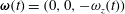 $\unicode[STIX]{x1D74E}(t)=(0,0,-\unicode[STIX]{x1D714}_{z}(t))$
. From (3.9), the torque
$\unicode[STIX]{x1D74E}(t)=(0,0,-\unicode[STIX]{x1D714}_{z}(t))$
. From (3.9), the torque
 $\boldsymbol{C}$
exerted by the fluid on the sphere when
$\boldsymbol{C}$
exerted by the fluid on the sphere when
 $\unicode[STIX]{x1D74E}(0)=\mathbf{0}$
is written as
$\unicode[STIX]{x1D74E}(0)=\mathbf{0}$
is written as
 $$\begin{eqnarray}\displaystyle \boldsymbol{C}(t) & = & \displaystyle 8\unicode[STIX]{x03C0}\unicode[STIX]{x1D707}a^{3}\left[\unicode[STIX]{x1D714}_{z}(t)+\frac{1}{3}\frac{a}{\sqrt{\unicode[STIX]{x03C0}\unicode[STIX]{x1D708}}}\int _{0}^{t}\frac{\text{d}\unicode[STIX]{x1D714}_{z}(t)}{\text{d}\unicode[STIX]{x1D70F}}\frac{1}{\sqrt{t-\unicode[STIX]{x1D70F}}}\,\text{d}\unicode[STIX]{x1D70F}\right.\nonumber\\ \displaystyle & & \displaystyle \left.-\,\frac{1}{3}\int _{0}^{t}\frac{\text{d}\unicode[STIX]{x1D714}_{z}(t)}{\text{d}\unicode[STIX]{x1D70F}}\exp \left(\frac{\unicode[STIX]{x1D708}(t-\unicode[STIX]{x1D70F})}{a^{2}}\right)\text{erfc}\left(\frac{\sqrt{\unicode[STIX]{x1D708}(t-\unicode[STIX]{x1D70F})}}{a}\right)\,\text{d}\unicode[STIX]{x1D70F}\right]\boldsymbol{e}_{\boldsymbol{z}}.\end{eqnarray}$$
Case 2 (the sphere is at rest). The fluid itself is in a time-dependent uniform shear flow
 $\boldsymbol{U}(\boldsymbol{x},t)=\dot{\unicode[STIX]{x1D6FE}}(t)y\boldsymbol{e}_{\boldsymbol{x}}$
. From (4.8), when
$\boldsymbol{U}(\boldsymbol{x},t)=\dot{\unicode[STIX]{x1D6FE}}(t)y\boldsymbol{e}_{\boldsymbol{x}}$
. From (4.8), when
 $\dot{\unicode[STIX]{x1D6FE}}(0)=0$
the torque
$\dot{\unicode[STIX]{x1D6FE}}(0)=0$
the torque
 $\boldsymbol{C}$
exerted by the fluid on the sphere:
$\boldsymbol{C}$
exerted by the fluid on the sphere:
 $$\begin{eqnarray}\displaystyle \boldsymbol{C}(t) & = & \displaystyle -4\unicode[STIX]{x03C0}\unicode[STIX]{x1D707}a^{3}\left[\dot{\unicode[STIX]{x1D6FE}}(t)+\frac{1}{3}\frac{a}{\sqrt{\unicode[STIX]{x03C0}\unicode[STIX]{x1D708}}}\int _{0}^{t}\frac{\text{d}\dot{\unicode[STIX]{x1D6FE}}(\unicode[STIX]{x1D70F})}{\,\text{d}\unicode[STIX]{x1D70F}}\frac{1}{\sqrt{t-\unicode[STIX]{x1D70F}}}\,\text{d}\unicode[STIX]{x1D70F}\right.\nonumber\\ \displaystyle & & \displaystyle \left.-\,\frac{1}{3}\int _{0}^{t}\frac{\text{d}\dot{\unicode[STIX]{x1D6FE}}(\unicode[STIX]{x1D70F})}{\text{d}\unicode[STIX]{x1D70F}}\exp \left(\frac{\unicode[STIX]{x1D708}(t-\unicode[STIX]{x1D70F})}{a^{2}}\right)\text{erfc}\left(\frac{\sqrt{\unicode[STIX]{x1D708}(t-\unicode[STIX]{x1D70F})}}{a}\right)\,\text{d}\unicode[STIX]{x1D70F}\right]\boldsymbol{e}_{\boldsymbol{z}}.\end{eqnarray}$$
Since the discussed problem of a sphere with free rotation in a simple shear flow is linear, by the superposition of (5.1) and (5.2); or by applying Faxén’s law, the time evolution of the sphere angular velocity is calculated by the following equation:
 $$\begin{eqnarray}\displaystyle & & \displaystyle -8\unicode[STIX]{x03C0}\unicode[STIX]{x1D707}a^{3}\left(\begin{array}{@{}l@{}}\displaystyle \left(\frac{\dot{\unicode[STIX]{x1D6FE}}(t)}{2}-\unicode[STIX]{x1D714}_{z}(t)\right)+\frac{1}{3}\frac{a}{\sqrt{\unicode[STIX]{x03C0}\unicode[STIX]{x1D708}}}\int _{0}^{t}\frac{\text{d}}{\text{d}\unicode[STIX]{x1D70F}}\left(\frac{\dot{\unicode[STIX]{x1D6FE}}(\unicode[STIX]{x1D70F})}{2}-\unicode[STIX]{x1D714}_{z}(t)\right)\frac{1}{\sqrt{t-\unicode[STIX]{x1D70F}}}\,\text{d}\unicode[STIX]{x1D70F}\\ \displaystyle -\,\frac{1}{3}\int _{0}^{t}\frac{\text{d}}{\text{d}\unicode[STIX]{x1D70F}}\left(\frac{\dot{\unicode[STIX]{x1D6FE}}(\unicode[STIX]{x1D70F})}{2}-\unicode[STIX]{x1D714}_{z}(t)\right)\exp \left(\frac{\unicode[STIX]{x1D708}(t-\unicode[STIX]{x1D70F})}{a^{2}}\right)\text{erfc}\left(\frac{\sqrt{\unicode[STIX]{x1D708}(t-\unicode[STIX]{x1D70F})}}{a}\right)\,\text{d}\unicode[STIX]{x1D70F}\end{array}\right)\nonumber\\ \displaystyle & & \displaystyle \quad =I\frac{\text{d}\unicode[STIX]{x1D714}_{z}(t)}{\text{d}t},\end{eqnarray}$$
where
 $I=2/5ma^{2}$
is the moment of inertia and
$I=2/5ma^{2}$
is the moment of inertia and
 $a$
,
$a$
,
 $m$
are the radius and mass of the sphere, respectively. We consider a steady shear flow, starting from a state of rest, i.e.
$m$
are the radius and mass of the sphere, respectively. We consider a steady shear flow, starting from a state of rest, i.e.
 $$\begin{eqnarray}\displaystyle \dot{\unicode[STIX]{x1D6FE}}(t)=\left\{\begin{array}{@{}ll@{}}0 & (t=0),\\ \unicode[STIX]{x1D6FE}_{\infty }=\text{constant} & (t\rightarrow \infty ).\end{array}\right. & & \displaystyle\end{eqnarray}$$
The rotation rate
 $\unicode[STIX]{x1D714}_{z}(t)$
of the sphere approaches its steady terminal value
$\unicode[STIX]{x1D714}_{z}(t)$
of the sphere approaches its steady terminal value
 $\unicode[STIX]{x1D714}_{z}=\text{constant}$
after a long time. Equation (5.3) then can be simplified to the steady result as
$\unicode[STIX]{x1D714}_{z}=\text{constant}$
after a long time. Equation (5.3) then can be simplified to the steady result as
 $$\begin{eqnarray}\displaystyle \unicode[STIX]{x1D714}_{z}={\textstyle \frac{1}{2}}\unicode[STIX]{x1D6FE}_{\infty }. & & \displaystyle\end{eqnarray}$$
The angular velocity
 $\unicode[STIX]{x1D714}_{z}$
will adjust to result in a vanishing hydrodynamic torque until a steady state is reached. In (5.5), the steady result was also a well-known solution obtained by Jeffery (Reference Jeffery1922) and Cox, Zia & Mason (Reference Cox, Zia and Mason1968) with a quasi-steady approach. On the other hand, if the shear rate
$\unicode[STIX]{x1D714}_{z}$
will adjust to result in a vanishing hydrodynamic torque until a steady state is reached. In (5.5), the steady result was also a well-known solution obtained by Jeffery (Reference Jeffery1922) and Cox, Zia & Mason (Reference Cox, Zia and Mason1968) with a quasi-steady approach. On the other hand, if the shear rate
 $\dot{\unicode[STIX]{x1D6FE}}(t)$
is forced theoretically to be
$\dot{\unicode[STIX]{x1D6FE}}(t)$
is forced theoretically to be
 $\dot{\unicode[STIX]{x1D6FE}}(t)=2\unicode[STIX]{x1D714}_{z}(t)$
in (5.3), thus the sphere rotates with a constant angular velocity
$\dot{\unicode[STIX]{x1D6FE}}(t)=2\unicode[STIX]{x1D714}_{z}(t)$
in (5.3), thus the sphere rotates with a constant angular velocity
 $\unicode[STIX]{x1D714}_{z}=\unicode[STIX]{x1D6FE}_{\infty }/2$
.
$\unicode[STIX]{x1D714}_{z}=\unicode[STIX]{x1D6FE}_{\infty }/2$
.

Figure 3. An axisymmetric parabolic flow
 $\boldsymbol{u}=K(t)(y^{2}+z^{2})\boldsymbol{e}_{\boldsymbol{x}}$
past a sphere of radius
$\boldsymbol{u}=K(t)(y^{2}+z^{2})\boldsymbol{e}_{\boldsymbol{x}}$
past a sphere of radius
 $a$
.
$a$
.
6 Axisymmetric parabolic flow past a sphere
We now consider an unbounded Stokes flow with the axisymmetric parabolic velocity profile
 $\boldsymbol{u}=K(t)(y^{2}+z^{2})\boldsymbol{e}_{\boldsymbol{x}}$
, past a sphere as depicted in figure 3. Following the lead of the steady case of Chwang & Wu (Reference Chwang and Wu1975), we employ an unsteady Stokeslet, an unsteady Stokeslet quadrupole, an unsteady potential dipole and an unsteady potential octupole with poles at the centre of the sphere, and construct the solutions. Then the induced velocity is expressed as a convolution integral in the following:
$\boldsymbol{u}=K(t)(y^{2}+z^{2})\boldsymbol{e}_{\boldsymbol{x}}$
, past a sphere as depicted in figure 3. Following the lead of the steady case of Chwang & Wu (Reference Chwang and Wu1975), we employ an unsteady Stokeslet, an unsteady Stokeslet quadrupole, an unsteady potential dipole and an unsteady potential octupole with poles at the centre of the sphere, and construct the solutions. Then the induced velocity is expressed as a convolution integral in the following:
 $$\begin{eqnarray}\displaystyle u_{i}(\boldsymbol{x},t) & = & \displaystyle K(t)(y^{2}+z^{2})\boldsymbol{e}_{\boldsymbol{x}}+\frac{1}{4\unicode[STIX]{x03C0}\unicode[STIX]{x1D70C}}\int _{0}^{t}G_{ij}^{S}(\hat{\boldsymbol{x}},t-\unicode[STIX]{x1D70F})\unicode[STIX]{x1D6FC}_{j}(\unicode[STIX]{x1D70F})\,\text{d}\unicode[STIX]{x1D70F}\nonumber\\ \displaystyle & & \displaystyle +\,\frac{1}{4\unicode[STIX]{x03C0}\unicode[STIX]{x1D70C}}\int _{0}^{t}G_{ijkl}^{SQ}(\hat{\boldsymbol{x}},t-\unicode[STIX]{x1D70F})Q_{jkl}(\unicode[STIX]{x1D70F})\,\text{d}\unicode[STIX]{x1D70F}+\frac{1}{4\unicode[STIX]{x03C0}}G_{ij}^{PD}(\hat{\boldsymbol{x}})d_{j}(t)\nonumber\\ \displaystyle & & \displaystyle +\,\frac{1}{4\unicode[STIX]{x03C0}}G_{ijkl}^{PO}(\hat{\boldsymbol{x}})O_{jkl}(t),\end{eqnarray}$$
where the second term on the right-hand side of (6.1) is an unsteady Stokeslet and the third term represents an unsteady Stokeslet quadrupole. The fourth term and last term are an unsteady potential dipole and an unsteady octupole. The
 $\unicode[STIX]{x1D6FC}_{j}(t),d_{j}(t),Q_{jkl}(t)$
, and
$\unicode[STIX]{x1D6FC}_{j}(t),d_{j}(t),Q_{jkl}(t)$
, and
 $O_{jkl}(t)$
are the time-dependent strengths of the unsteady singularities for unsteady Stokeslet, unsteady Stokeslet quadrupole, unsteady potential dipole and unsteady potential octupole, respectively. Moreover, the fundamental solutions of
$O_{jkl}(t)$
are the time-dependent strengths of the unsteady singularities for unsteady Stokeslet, unsteady Stokeslet quadrupole, unsteady potential dipole and unsteady potential octupole, respectively. Moreover, the fundamental solutions of
 $G_{ij}^{S}(\hat{\boldsymbol{x}},t)$
and
$G_{ij}^{S}(\hat{\boldsymbol{x}},t)$
and
 $G_{ijkl}^{SQ}(\hat{\boldsymbol{x}},t)$
can be found in (2.3) and (2.32). Next, a potential octupole has been presented in (2.37). The boundary conditions are
$G_{ijkl}^{SQ}(\hat{\boldsymbol{x}},t)$
can be found in (2.3) and (2.32). Next, a potential octupole has been presented in (2.37). The boundary conditions are
 $$\begin{eqnarray}\displaystyle \boldsymbol{u}=\mathbf{0}\quad \text{at}~r=a. & & \displaystyle\end{eqnarray}$$
After applying the boundary conditions and taking the Laplace transform of (6.1), we obtain four equations for the coefficients of the singularities (listed in appendix C). After solving the system, we obtain the unknown strengths of
 $\hat{\unicode[STIX]{x1D6FC}}_{1}(s),\hat{d}_{1}(s),\hat{Q}_{111}(s)$
and
$\hat{\unicode[STIX]{x1D6FC}}_{1}(s),\hat{d}_{1}(s),\hat{Q}_{111}(s)$
and
 $\hat{O} _{111}(s)$
in the Laplace domain as given by
$\hat{O} _{111}(s)$
in the Laplace domain as given by
 $$\begin{eqnarray}\displaystyle & \displaystyle \hat{\unicode[STIX]{x1D6FC}}_{1}(s)=-K(s)\left(4\unicode[STIX]{x03C0}\unicode[STIX]{x1D707}a^{3}+\frac{7}{15}\unicode[STIX]{x03C0}\unicode[STIX]{x1D70C}a^{5}\frac{s}{\left(1+\displaystyle \frac{a}{\sqrt{\unicode[STIX]{x1D708}}}\sqrt{s}+\frac{a^{2}}{3\unicode[STIX]{x1D708}}s\right)}\right)\exp (\sqrt{a^{2}s/\unicode[STIX]{x1D708}}), & \displaystyle\end{eqnarray}$$
 $$\begin{eqnarray}\displaystyle & \displaystyle \hat{Q}_{111}(s)=\frac{7}{3}K(s)\unicode[STIX]{x03C0}\unicode[STIX]{x1D707}a^{5}\frac{1}{\left(1+\displaystyle \frac{a}{\sqrt{\unicode[STIX]{x1D708}}}\sqrt{s}+\frac{a^{2}}{3\unicode[STIX]{x1D708}}s\right)}\exp (\sqrt{a^{2}s/\unicode[STIX]{x1D708}}), & \displaystyle\end{eqnarray}$$
 $$\begin{eqnarray}\displaystyle \hat{d}_{1}(s) & = & \displaystyle -K(s)\left(4\unicode[STIX]{x03C0}a^{4}\sqrt{\unicode[STIX]{x1D708}}\frac{1}{\sqrt{s}}+4\unicode[STIX]{x03C0}a^{3}\unicode[STIX]{x1D708}\frac{1}{s}+\frac{4}{5}\unicode[STIX]{x03C0}a^{5}\right)\nonumber\\ \displaystyle & & \displaystyle +\,K(s)\left(4\unicode[STIX]{x03C0}\unicode[STIX]{x1D708}a^{3}\frac{1}{s}+\frac{7}{15}\unicode[STIX]{x03C0}a^{5}\frac{1}{\left(1+\displaystyle \frac{a}{\sqrt{\unicode[STIX]{x1D708}}}\sqrt{s}+\frac{a^{2}}{3\unicode[STIX]{x1D708}}s\right)}\right)\exp (\sqrt{a^{2}s/\unicode[STIX]{x1D708}}),\end{eqnarray}$$
 $$\begin{eqnarray}\displaystyle \hat{O} _{111}(s)=K(s)\left\{\begin{array}{@{}l@{}}\displaystyle \frac{7}{3}\frac{\unicode[STIX]{x03C0}a^{6}\sqrt{\unicode[STIX]{x1D708}}}{\sqrt{s}\left(\displaystyle 1+\frac{a}{\sqrt{\unicode[STIX]{x1D708}}}\sqrt{s}+\frac{a^{2}}{3\unicode[STIX]{x1D708}}s\right)}+\frac{\unicode[STIX]{x03C0}a^{7}}{\left(1+\displaystyle \frac{a}{\sqrt{\unicode[STIX]{x1D708}}}\sqrt{s}+\frac{a^{2}}{3\unicode[STIX]{x1D708}}s\right)}\\ \displaystyle +\,\frac{2}{9}\frac{\unicode[STIX]{x03C0}a^{8}\unicode[STIX]{x1D708}^{-1/2}\sqrt{s}}{\left(1+\displaystyle \frac{a}{\sqrt{\unicode[STIX]{x1D708}}}\sqrt{s}+\frac{a^{2}}{3\unicode[STIX]{x1D708}}s\right)}+\frac{1}{45}\frac{\unicode[STIX]{x03C0}a^{9}\unicode[STIX]{x1D708}^{-1}s}{\left(1+\displaystyle \frac{a}{\sqrt{\unicode[STIX]{x1D708}}}\sqrt{s}+\frac{a^{2}}{3\unicode[STIX]{x1D708}}s\right)}\\ \displaystyle +\,\frac{7}{3}\frac{\unicode[STIX]{x03C0}\unicode[STIX]{x1D708}a^{5}}{\left(1+\displaystyle \frac{a}{\sqrt{\unicode[STIX]{x1D708}}}\sqrt{s}+\frac{a^{2}}{3\unicode[STIX]{x1D708}}s\right)}\left(\frac{1-\exp (\sqrt{a^{2}s/\unicode[STIX]{x1D708}})}{s}\right)\end{array}\right\}. & & \displaystyle\end{eqnarray}$$
If
 $K(t)$
is bounded and
$K(t)$
is bounded and
 $\lim _{t\rightarrow \infty }K(t)=K_{\infty }$
, by using the final value theorem of the Laplace transform, the steady strengths of an unsteady Stokeslet, an unsteady potential dipole, an unsteady Stokeslet quadrupole and an unsteady potential octupole in (6.3), (6.4), (6.5) and (6.6) are calculated as
$\lim _{t\rightarrow \infty }K(t)=K_{\infty }$
, by using the final value theorem of the Laplace transform, the steady strengths of an unsteady Stokeslet, an unsteady potential dipole, an unsteady Stokeslet quadrupole and an unsteady potential octupole in (6.3), (6.4), (6.5) and (6.6) are calculated as
 $$\begin{eqnarray}\displaystyle \lim _{s\rightarrow 0}\frac{s\hat{\unicode[STIX]{x1D6FC}}_{1}(s)}{8\unicode[STIX]{x03C0}\unicode[STIX]{x1D707}}=\lim _{t\rightarrow \infty }\frac{\unicode[STIX]{x1D6FC}_{1}(t)}{8\unicode[STIX]{x03C0}\unicode[STIX]{x1D707}}=-\frac{1}{2}K_{\infty }a^{3},\quad \lim _{s\rightarrow 0}\frac{s\hat{d}_{1}(s)}{4\unicode[STIX]{x03C0}}=\lim _{t\rightarrow \infty }\frac{d_{1}(t)}{4\unicode[STIX]{x03C0}}=\frac{5}{12}K_{\infty }a^{5} & & \displaystyle\end{eqnarray}$$
and
 $$\begin{eqnarray}\displaystyle \lim _{s\rightarrow 0}\frac{s\hat{Q}_{111}(s)}{8\unicode[STIX]{x03C0}\unicode[STIX]{x1D707}}=\lim _{t\rightarrow \infty }\frac{Q_{111}(t)}{8\unicode[STIX]{x03C0}\unicode[STIX]{x1D707}}=\frac{7}{24}K_{\infty }a^{5},\quad \lim _{s\rightarrow 0}\frac{s\hat{O} _{111}(s)}{4\unicode[STIX]{x03C0}}=\lim _{t\rightarrow \infty }\frac{O_{111}(t)}{4\unicode[STIX]{x03C0}}=-\frac{1}{24}K_{\infty }a^{7}. & & \displaystyle \nonumber\\ \displaystyle & & \displaystyle\end{eqnarray}$$
In summary the results are all in agreement with the equations obtained by Chwang & Wu (Reference Chwang and Wu1975, p. 807, (68b)). It is also noted that the signs of
 $-1/2Ka^{3}$
and
$-1/2Ka^{3}$
and
 $-1/24Ka^{7}$
are due to the coefficients
$-1/24Ka^{7}$
are due to the coefficients
 $-C_{1}$
and
$-C_{1}$
and
 $-C_{4}$
(Chwang & Wu Reference Chwang and Wu1975, p. 806, (68a)).
$-C_{4}$
(Chwang & Wu Reference Chwang and Wu1975, p. 806, (68a)).
From (6.1), the absence of rotary singularities results in zero net torque. However, it is interesting to note that the hydrodynamic force is due to an unsteady Stokeslet and an unsteady potential dipole. In the next §§ 6.1 and 6.2, we are going to compute the hydrodynamic force induced by these two singularities for the problem of a sphere in a parabolic flow.
6.1 Contribution of the unsteady Stokeslet
The force contribution from the unsteady Stokeslet can be decomposed as viscous and pressure parts
 $\boldsymbol{F}_{\boldsymbol{s}}(t)=\boldsymbol{F}_{\boldsymbol{s},\boldsymbol{v}}(t)+\boldsymbol{F}_{\boldsymbol{s},\boldsymbol{p}}(t)$
. In order to obtain the viscous force
$\boldsymbol{F}_{\boldsymbol{s}}(t)=\boldsymbol{F}_{\boldsymbol{s},\boldsymbol{v}}(t)+\boldsymbol{F}_{\boldsymbol{s},\boldsymbol{p}}(t)$
. In order to obtain the viscous force
 $\boldsymbol{F}_{\boldsymbol{s},\boldsymbol{v}}(t)$
, we can use the first term on the right-hand side in (2.5) which shows that the viscous force exerted by an unsteady Stokeslet on the sphere in time
$\boldsymbol{F}_{\boldsymbol{s},\boldsymbol{v}}(t)$
, we can use the first term on the right-hand side in (2.5) which shows that the viscous force exerted by an unsteady Stokeslet on the sphere in time
 $t$
, and the convolution integral will yield
$t$
, and the convolution integral will yield
 $$\begin{eqnarray}\displaystyle \boldsymbol{F}_{\boldsymbol{s},\boldsymbol{v}}(t)=-\int _{0}^{t}\frac{\unicode[STIX]{x1D736}(\unicode[STIX]{x1D70F})}{\sqrt{\unicode[STIX]{x03C0}\unicode[STIX]{x1D708}}}\left(\frac{a^{3}}{6\unicode[STIX]{x1D708}}\right)\frac{\exp \left(-\displaystyle \frac{a^{2}}{4\unicode[STIX]{x1D708}(t-\unicode[STIX]{x1D70F})}\right)}{(t-\unicode[STIX]{x1D70F})^{5/2}}\,\text{d}\unicode[STIX]{x1D70F}. & & \displaystyle\end{eqnarray}$$
Taking the Laplace transform of both sides, we have
 $$\begin{eqnarray}\displaystyle \boldsymbol{F}_{\boldsymbol{s},\boldsymbol{v}}(s)=-\frac{2}{3}\hat{\unicode[STIX]{x1D736}}(s)\left(1+\frac{a}{\sqrt{\unicode[STIX]{x1D708}}}\sqrt{s}\right)\exp (-\sqrt{a^{2}s/\unicode[STIX]{x1D708}}). & & \displaystyle\end{eqnarray}$$
By substituting
 $\hat{\unicode[STIX]{x1D6FC}}_{1}(s)$
of (6.3) into (6.10), we get
$\hat{\unicode[STIX]{x1D6FC}}_{1}(s)$
of (6.3) into (6.10), we get
 $$\begin{eqnarray}\displaystyle \boldsymbol{F}_{\boldsymbol{s},\boldsymbol{v}}(s)=\left\{\frac{8}{3}\unicode[STIX]{x03C0}\unicode[STIX]{x1D707}a^{3}K(s)+\frac{8}{3}\unicode[STIX]{x03C0}\unicode[STIX]{x1D70C}a^{4}\sqrt{\unicode[STIX]{x1D708}}\sqrt{s}K(s)+\frac{14}{45}\unicode[STIX]{x03C0}\unicode[STIX]{x1D70C}a^{5}\frac{s\left(1+\displaystyle \frac{a}{\sqrt{\unicode[STIX]{x1D708}}}\sqrt{s}\right)}{1+\displaystyle \frac{a}{\sqrt{\unicode[STIX]{x1D708}}}\sqrt{s}+\frac{a^{2}}{3\unicode[STIX]{x1D708}}s}K(s)\right\}\boldsymbol{e}_{\boldsymbol{x}}. & & \displaystyle \nonumber\\ \displaystyle & & \displaystyle\end{eqnarray}$$
Using the convolution theorem and inverse Laplace transform (solved in appendix D), equation (6.11) including the initial condition becomes
 $$\begin{eqnarray}\displaystyle \boldsymbol{F}_{\boldsymbol{s},\boldsymbol{v}}(t) & = & \displaystyle \left\{\frac{8}{3}\unicode[STIX]{x03C0}\unicode[STIX]{x1D707}a^{3}K(t)+\frac{8}{3}\unicode[STIX]{x03C0}\unicode[STIX]{x1D70C}a^{4}\sqrt{\frac{\unicode[STIX]{x1D708}}{\unicode[STIX]{x03C0}}}\int _{0}^{t}\frac{\text{d}K}{\text{d}\unicode[STIX]{x1D70F}}\frac{1}{\sqrt{t-\unicode[STIX]{x1D70F}}}\,\text{d}\unicode[STIX]{x1D70F}\right.\nonumber\\ \displaystyle & & \displaystyle +\,\frac{28\sqrt{3}}{45}\unicode[STIX]{x03C0}\unicode[STIX]{x1D70C}a^{4}\sqrt{\frac{\unicode[STIX]{x1D708}}{\unicode[STIX]{x03C0}}}\int _{0}^{t}\frac{\text{d}K}{\text{d}\unicode[STIX]{x1D70F}}S_{F1}(t-\unicode[STIX]{x1D70F})\,\text{d}\unicode[STIX]{x1D70F}+\frac{28\sqrt{3}}{45}\unicode[STIX]{x03C0}\unicode[STIX]{x1D70C}a^{5}\int _{0}^{t}\frac{\text{d}^{2}K}{\text{d}\unicode[STIX]{x1D70F}^{2}}S_{F2}(t-\unicode[STIX]{x1D70F})\,\text{d}\unicode[STIX]{x1D70F}\nonumber\\ \displaystyle & & \displaystyle +\,\frac{8}{3}\unicode[STIX]{x03C0}\unicode[STIX]{x1D70C}a^{4}\sqrt{\frac{\unicode[STIX]{x1D708}}{\unicode[STIX]{x03C0}}}K(0)\frac{1}{\sqrt{t}}+\frac{28\sqrt{3}}{45}\unicode[STIX]{x03C0}\unicode[STIX]{x1D70C}a^{4}\sqrt{\frac{\unicode[STIX]{x1D708}}{\unicode[STIX]{x03C0}}}K(0)S_{F1}(t)\nonumber\\ \displaystyle & & \displaystyle \left.+\,\frac{28\sqrt{3}}{45}\unicode[STIX]{x03C0}\unicode[STIX]{x1D70C}a^{5}\left(K(0)\frac{\text{d}}{\text{d}t}(S_{F2}(t))+\left.\frac{\text{d}K}{\text{d}t}\right|_{t=0}S_{F2}(t)\right)\right\}\boldsymbol{e}_{\boldsymbol{x}},\end{eqnarray}$$
where
 $$\begin{eqnarray}\displaystyle \left.\begin{array}{@{}c@{}}\displaystyle S_{F1}(t)=\text{Im}\left(\sqrt{\unicode[STIX]{x03C0}}\left(\frac{\sqrt{\unicode[STIX]{x1D708}}\unicode[STIX]{x1D6FD}}{a}\right)\text{e}^{(\unicode[STIX]{x1D708}/a^{2})\unicode[STIX]{x1D6FD}^{2}t}\text{erfc}\left(\frac{\sqrt{\unicode[STIX]{x1D708}}\unicode[STIX]{x1D6FD}}{a}\sqrt{t}\right)\right),\\ \displaystyle S_{F2}(t)=-\text{Im}\left(\text{e}^{(\unicode[STIX]{x1D707}/a^{2})\unicode[STIX]{x1D6FD}^{2}t}\text{erfc}\left(\frac{\sqrt{\unicode[STIX]{x1D708}}\unicode[STIX]{x1D6FD}}{a}\sqrt{t}\right)\right),\quad \text{and}\quad \unicode[STIX]{x1D6FD}=\frac{3}{2}+\frac{\sqrt{3}}{2}\text{i}.\end{array}\right\} & & \displaystyle\end{eqnarray}$$
To determine the pressure force
 $\boldsymbol{F}_{\boldsymbol{s},\boldsymbol{p}}(t)$
, we note that the second term on the right-hand side in (2.5) shows the pressure exerted by an unsteady Stokeslet. We substitute
$\boldsymbol{F}_{\boldsymbol{s},\boldsymbol{p}}(t)$
, we note that the second term on the right-hand side in (2.5) shows the pressure exerted by an unsteady Stokeslet. We substitute
 $\hat{\unicode[STIX]{x1D6FC}}_{1}(s)$
of (6.3) into the second term in (2.5) and use the convolution integral to obtain
$\hat{\unicode[STIX]{x1D6FC}}_{1}(s)$
of (6.3) into the second term in (2.5) and use the convolution integral to obtain
 $$\begin{eqnarray}\displaystyle \boldsymbol{F}_{\boldsymbol{s},\boldsymbol{p}}(t)=-\frac{1}{3}\int _{0}^{t}\unicode[STIX]{x1D6FC}_{1}(\unicode[STIX]{x1D70F})\unicode[STIX]{x1D6FF}(t-\unicode[STIX]{x1D70F})\,\text{d}\unicode[STIX]{x1D70F}\boldsymbol{e}_{\boldsymbol{x}}=-\frac{1}{3}\unicode[STIX]{x1D6FC}_{1}(t)\boldsymbol{e}_{\boldsymbol{x}}. & & \displaystyle\end{eqnarray}$$
Therefore, the total force acting on the sphere due to an unsteady Stokeslet is the summation of (6.12) and (6.14) as follows:
 $$\begin{eqnarray}\displaystyle \boldsymbol{F}_{\boldsymbol{s}}(t) & = & \displaystyle \boldsymbol{F}_{\boldsymbol{s},\boldsymbol{v}}(t)+\boldsymbol{F}_{\boldsymbol{s},\boldsymbol{p}}(t)\nonumber\\ \displaystyle & = & \displaystyle \left\{\frac{8}{3}\unicode[STIX]{x03C0}\unicode[STIX]{x1D707}a^{3}K(t)+\frac{8}{3}\unicode[STIX]{x03C0}\unicode[STIX]{x1D70C}a^{4}\sqrt{\frac{\unicode[STIX]{x1D708}}{\unicode[STIX]{x03C0}}}\int _{0}^{t}\frac{\text{d}K}{\text{d}\unicode[STIX]{x1D70F}}\frac{1}{\sqrt{t-\unicode[STIX]{x1D70F}}}\,\text{d}\unicode[STIX]{x1D70F}\right.\nonumber\\ \displaystyle & & \displaystyle +\,\frac{28\sqrt{3}}{45}\unicode[STIX]{x03C0}\unicode[STIX]{x1D70C}a^{4}\sqrt{\frac{\unicode[STIX]{x1D708}}{\unicode[STIX]{x03C0}}}\int _{0}^{t}\frac{\text{d}K}{\text{d}\unicode[STIX]{x1D70F}}S_{F1}(t-\unicode[STIX]{x1D70F})\,\text{d}\unicode[STIX]{x1D70F}+\frac{28\sqrt{3}}{45}\unicode[STIX]{x03C0}\unicode[STIX]{x1D70C}a^{5}\int _{0}^{t}\frac{\text{d}^{2}K}{\text{d}\unicode[STIX]{x1D70F}^{2}}S_{F2}(t-\unicode[STIX]{x1D70F})\,\text{d}\unicode[STIX]{x1D70F}\nonumber\\ \displaystyle & & \displaystyle +\,\frac{8}{3}\unicode[STIX]{x03C0}\unicode[STIX]{x1D70C}a^{4}\sqrt{\frac{\unicode[STIX]{x1D708}}{\unicode[STIX]{x03C0}}}K(0)\frac{1}{\sqrt{t}}+\frac{28\sqrt{3}}{45}\unicode[STIX]{x03C0}\unicode[STIX]{x1D70C}a^{4}\sqrt{\frac{\unicode[STIX]{x1D708}}{\unicode[STIX]{x03C0}}}K(0)S_{F1}(t)\nonumber\\ \displaystyle & & \displaystyle \left.+\,\frac{28\sqrt{3}}{45}\unicode[STIX]{x03C0}\unicode[STIX]{x1D70C}a^{5}\left(K(0)\frac{d}{dt}(S_{F2}(t))+\left.\frac{\text{d}K}{\text{d}t}\right|_{t=0}S_{F2}(t)\right)-\frac{1}{3}\unicode[STIX]{x1D6FC}_{1}(t)\right\}\boldsymbol{e}_{\boldsymbol{x}}.\end{eqnarray}$$
6.2 Contribution of the unsteady potential dipole
The surrounding fluid exerts a force on the sphere of radius
 $a$
centred at an unsteady potential dipole as (appendix A, equation (A 7))
$a$
centred at an unsteady potential dipole as (appendix A, equation (A 7))
 $$\begin{eqnarray}\displaystyle F_{i}(t)=-\frac{\unicode[STIX]{x1D70C}}{3}\frac{\text{d}}{\text{d}t}(d_{i}(t)). & & \displaystyle\end{eqnarray}$$
By taking the Laplace transform of (6.16), the surface force due to an unsteady potential dipole in the Laplace transform domain is
 $$\begin{eqnarray}\displaystyle \hat{F}_{i}(s)=-\frac{\unicode[STIX]{x1D70C}}{3}s\hat{d}_{i}(s). & & \displaystyle\end{eqnarray}$$
Substituting
 $\hat{d}_{1}(s)$
of (6.5) into (6.17) and making use of (6.3), we get
$\hat{d}_{1}(s)$
of (6.5) into (6.17) and making use of (6.3), we get
 $$\begin{eqnarray}\displaystyle \hat{\boldsymbol{F}}_{\boldsymbol{d}}(s)=\left\{\frac{4}{3}\unicode[STIX]{x03C0}\unicode[STIX]{x1D707}a^{3}K(s)+\frac{4}{15}\unicode[STIX]{x03C0}\unicode[STIX]{x1D70C}a^{5}sK(s)+\frac{4}{3}\unicode[STIX]{x03C0}\unicode[STIX]{x1D70C}a^{4}\sqrt{\unicode[STIX]{x1D708}}\sqrt{s}K(s)+\frac{1}{3}\hat{\unicode[STIX]{x1D6FC}}_{1}(s)\right\}\boldsymbol{e}_{\boldsymbol{x}}. & & \displaystyle\end{eqnarray}$$
Using the inverse Laplace transform, we obtain
 $$\begin{eqnarray}\displaystyle \boldsymbol{F}_{\boldsymbol{d}}(t) & = & \displaystyle \left\{\frac{4}{3}\unicode[STIX]{x03C0}\unicode[STIX]{x1D707}a^{3}K(t)+\frac{4}{15}\unicode[STIX]{x03C0}\unicode[STIX]{x1D70C}a^{5}\frac{\text{d}K}{\text{d}t}+\frac{4}{3}\unicode[STIX]{x03C0}\unicode[STIX]{x1D70C}a^{4}\sqrt{\frac{\unicode[STIX]{x1D708}}{\unicode[STIX]{x03C0}}}\int _{0}^{t}\frac{\text{d}K}{\text{d}\unicode[STIX]{x1D70F}}\frac{1}{\sqrt{t-\unicode[STIX]{x1D70F}}}\,\text{d}\unicode[STIX]{x1D70F}+\frac{1}{3}\unicode[STIX]{x1D6FC}_{1}(t)\right.\nonumber\\ \displaystyle & & \displaystyle \left.+\,\frac{4}{15}\unicode[STIX]{x03C0}\unicode[STIX]{x1D70C}a^{5}K(0)+\frac{4}{3}\unicode[STIX]{x03C0}\unicode[STIX]{x1D70C}a^{4}\sqrt{\frac{\unicode[STIX]{x1D708}}{\unicode[STIX]{x03C0}}}K(0)\frac{1}{\sqrt{t}}\right\}\boldsymbol{e}_{\boldsymbol{x}}.\end{eqnarray}$$
It should be mentioned that an unsteady Stokeslet quadrupole and an unsteady potential octupole result in no net force and no net torque to the fluid due to the symmetry property.
6.3 Net hydrodynamic force on the sphere
By combining (6.15) and (6.19), we finally have the hydrodynamic force on the sphere as
 $$\begin{eqnarray}\displaystyle \boldsymbol{F} & = & \displaystyle \left\{4\unicode[STIX]{x03C0}\unicode[STIX]{x1D707}a^{3}K(t)+\frac{4}{15}\unicode[STIX]{x03C0}\unicode[STIX]{x1D70C}a^{5}\frac{\text{d}K}{\text{d}t}+4\unicode[STIX]{x03C0}\unicode[STIX]{x1D70C}a^{4}\sqrt{\frac{\unicode[STIX]{x1D708}}{\unicode[STIX]{x03C0}}}\int _{0}^{t}\frac{\text{d}K}{\text{d}\unicode[STIX]{x1D70F}}\frac{1}{\sqrt{t-\unicode[STIX]{x1D70F}}}\,\text{d}\unicode[STIX]{x1D70F}\right.\nonumber\\ \displaystyle & & \displaystyle +\,\frac{28\sqrt{3}}{45}\unicode[STIX]{x03C0}\unicode[STIX]{x1D70C}a^{4}\sqrt{\frac{\unicode[STIX]{x1D708}}{\unicode[STIX]{x03C0}}}\int _{0}^{t}\frac{\text{d}K}{\text{d}\unicode[STIX]{x1D70F}}S_{F1}(t-\unicode[STIX]{x1D70F})\,\text{d}\unicode[STIX]{x1D70F}+\frac{28\sqrt{3}}{45}\unicode[STIX]{x03C0}\unicode[STIX]{x1D70C}a^{5}\int _{0}^{t}\frac{\text{d}^{2}K}{\text{d}\unicode[STIX]{x1D70F}^{2}}S_{F2}(t-\unicode[STIX]{x1D70F})\,\text{d}\unicode[STIX]{x1D70F}\nonumber\\ \displaystyle & & \displaystyle +\,\frac{4}{15}\unicode[STIX]{x03C0}\unicode[STIX]{x1D70C}a^{5}K(0)+4\unicode[STIX]{x03C0}\unicode[STIX]{x1D70C}a^{4}\sqrt{\frac{\unicode[STIX]{x1D708}}{\unicode[STIX]{x03C0}}}K(0)\frac{1}{\sqrt{t}}\nonumber\\ \displaystyle & & \displaystyle +\,\frac{28\sqrt{3}}{45}\unicode[STIX]{x03C0}\unicode[STIX]{x1D70C}a^{4}\sqrt{\frac{\unicode[STIX]{x1D708}}{\unicode[STIX]{x03C0}}}K(0)S_{F1}(t)\nonumber\\ \displaystyle & & \displaystyle \left.+\,\frac{28\sqrt{3}}{45}\unicode[STIX]{x03C0}\unicode[STIX]{x1D70C}a^{5}\left(K(0)\frac{\text{d}}{\text{d}t}(S_{F2}(t))+\left.\frac{\text{d}K}{\text{d}t}\right|_{t=0}S_{F2}(t)\right)\right\}\boldsymbol{e}_{\boldsymbol{x}}.\end{eqnarray}$$
For steady Stokes flow, the drag on the sphere when the ambient field has a paraboloidal profile with the axis passing through the centre of the sphere is the same as that on the same sphere moves with an ‘equivalent velocity’ in a uniform flow (Chwang & Wu Reference Chwang and Wu1975). The role is based on the calculation of drag force. In (6.20), we follow the equivalent velocity in steady Stokes flow given by Chwang & Wu (Reference Chwang and Wu1975) to put it in the following form:
 $$\begin{eqnarray}\displaystyle \boldsymbol{U}_{\boldsymbol{e}}=\frac{2}{3}K(t)a^{2}\boldsymbol{e}_{\boldsymbol{ x}}. & & \displaystyle\end{eqnarray}$$
Therefore, equation (6.20) can be rewritten in an equivalent velocity form:
 $$\begin{eqnarray}\displaystyle \boldsymbol{F} & = & \displaystyle 6\unicode[STIX]{x03C0}\unicode[STIX]{x1D707}a\boldsymbol{U}_{\boldsymbol{e}}(t)+\frac{2}{5}\unicode[STIX]{x03C0}a^{3}\unicode[STIX]{x1D70C}\frac{\text{d}\boldsymbol{U}_{\boldsymbol{e}}}{\text{d}t}+6\unicode[STIX]{x03C0}\unicode[STIX]{x1D70C}a^{2}\sqrt{\frac{\unicode[STIX]{x1D708}}{\unicode[STIX]{x03C0}}}\int _{0}^{t}\frac{\text{d}\boldsymbol{U}_{\boldsymbol{e}}}{\text{d}\unicode[STIX]{x1D70F}}\frac{1}{\sqrt{t-\unicode[STIX]{x1D70F}}}\,\text{d}\unicode[STIX]{x1D70F}\nonumber\\ \displaystyle & & \displaystyle +\,\frac{14\sqrt{3}}{15}\unicode[STIX]{x03C0}\unicode[STIX]{x1D70C}a^{2}\sqrt{\frac{\unicode[STIX]{x1D708}}{\unicode[STIX]{x03C0}}}\int _{0}^{t}\frac{\text{d}\boldsymbol{U}_{\boldsymbol{e}}}{\text{d}\unicode[STIX]{x1D70F}}S_{F1}(t-\unicode[STIX]{x1D70F})\,\text{d}\unicode[STIX]{x1D70F}+\frac{14\sqrt{3}}{15}\unicode[STIX]{x03C0}\unicode[STIX]{x1D70C}a^{3}\int _{0}^{t}\frac{\text{d}^{2}\boldsymbol{U}_{\boldsymbol{ e}}}{\text{d}\unicode[STIX]{x1D70F}^{2}}S_{F2}(t-\unicode[STIX]{x1D70F})\,\text{d}\unicode[STIX]{x1D70F}\nonumber\\ \displaystyle & & \displaystyle +\,\frac{2}{5}\unicode[STIX]{x03C0}a^{3}\unicode[STIX]{x1D70C}\boldsymbol{U}_{\boldsymbol{ e}}(0)+6\unicode[STIX]{x03C0}\unicode[STIX]{x1D70C}a^{2}\sqrt{\frac{\unicode[STIX]{x1D708}}{\unicode[STIX]{x03C0}}}\boldsymbol{U}_{\boldsymbol{ e}}(0)\frac{1}{\sqrt{t}}\nonumber\\ \displaystyle & & \displaystyle +\,\frac{14\sqrt{3}}{15}\unicode[STIX]{x03C0}\unicode[STIX]{x1D70C}a^{2}\sqrt{\frac{\unicode[STIX]{x1D708}}{\unicode[STIX]{x03C0}}}\boldsymbol{U}_{\boldsymbol{ e}}(0)S_{F1}(t)\nonumber\\ \displaystyle & & \displaystyle +\,\frac{14\sqrt{3}}{15}\unicode[STIX]{x03C0}\unicode[STIX]{x1D70C}a^{3}\left(\boldsymbol{U}_{\boldsymbol{ e}}(0)\frac{\text{d}}{\text{d}t}(S_{F2}(t))+\left.\frac{\text{d}\boldsymbol{U}_{\boldsymbol{e}}}{\text{d}t}\right|_{t=0}S_{F2}(t)\right).\end{eqnarray}$$
Equation (6.22) is compared with (1.1), when
 $\boldsymbol{U}_{\boldsymbol{e}}(0)=\mathbf{0}$
and
$\boldsymbol{U}_{\boldsymbol{e}}(0)=\mathbf{0}$
and
 $\text{d}\boldsymbol{U}_{\boldsymbol{e}}/\text{d}t_{t=0}=\mathbf{0}$
is taken. It shows that the rule is not hydrodynamically equivalent in unsteady Stokes flow. The first three terms of (6.22) are the standard forms for the quasi-steady Stokes drag force, added mass force and Basset force term, respectively. But results also show that the coefficient of added mass force of (6.22) does not correspond to (1.1). It should be noted that a very important feature of the result is to produce two additional memory force terms in addition to the Basset memory force. The fourth term, like the Basset force, is a memory force integral. More specifically, comparing (1.3) with (6.12) and (6.13), it is surprising that the kernel function
$\text{d}\boldsymbol{U}_{\boldsymbol{e}}/\text{d}t_{t=0}=\mathbf{0}$
is taken. It shows that the rule is not hydrodynamically equivalent in unsteady Stokes flow. The first three terms of (6.22) are the standard forms for the quasi-steady Stokes drag force, added mass force and Basset force term, respectively. But results also show that the coefficient of added mass force of (6.22) does not correspond to (1.1). It should be noted that a very important feature of the result is to produce two additional memory force terms in addition to the Basset memory force. The fourth term, like the Basset force, is a memory force integral. More specifically, comparing (1.3) with (6.12) and (6.13), it is surprising that the kernel function
 $S_{F1}(t)$
is also found in the hydrodynamic force on a slightly deformed translating spheroid given by Lawrence & Weinbaum (Reference Lawrence and Weinbaum1986), and where the constants
$S_{F1}(t)$
is also found in the hydrodynamic force on a slightly deformed translating spheroid given by Lawrence & Weinbaum (Reference Lawrence and Weinbaum1986), and where the constants
 $\sqrt{\unicode[STIX]{x1D702}}=\unicode[STIX]{x1D6FD}$
. In addition, when the flow starts from rest, the initial condition at
$\sqrt{\unicode[STIX]{x1D702}}=\unicode[STIX]{x1D6FD}$
. In addition, when the flow starts from rest, the initial condition at
 $t=0$
,
$t=0$
,
 $K=\text{d}K(t)/\text{d}t=0$
, is applied and (6.22) is simply reduced to
$K=\text{d}K(t)/\text{d}t=0$
, is applied and (6.22) is simply reduced to
 $$\begin{eqnarray}\displaystyle \boldsymbol{F} & = & \displaystyle 6\unicode[STIX]{x03C0}\unicode[STIX]{x1D707}a\boldsymbol{U}_{\boldsymbol{e}}(t)+\frac{2}{5}\unicode[STIX]{x03C0}a^{3}\unicode[STIX]{x1D70C}\frac{\text{d}\boldsymbol{U}_{\boldsymbol{e}}}{\text{d}t}+6\unicode[STIX]{x03C0}\unicode[STIX]{x1D70C}a^{2}\sqrt{\frac{\unicode[STIX]{x1D708}}{\unicode[STIX]{x03C0}}}\int _{0}^{t}\frac{\text{d}\boldsymbol{U}_{\boldsymbol{e}}}{\text{d}\unicode[STIX]{x1D70F}}\frac{1}{\sqrt{t-\unicode[STIX]{x1D70F}}}\,\text{d}\unicode[STIX]{x1D70F}\nonumber\\ \displaystyle & & \displaystyle +\,\frac{14\sqrt{3}}{15}\unicode[STIX]{x03C0}\unicode[STIX]{x1D70C}a^{2}\sqrt{\frac{\unicode[STIX]{x1D708}}{\unicode[STIX]{x03C0}}}\int _{0}^{t}\frac{\text{d}\boldsymbol{U}_{\boldsymbol{e}}}{\text{d}\unicode[STIX]{x1D70F}}S_{F1}(t-\unicode[STIX]{x1D70F})\,\text{d}\unicode[STIX]{x1D70F}+\frac{14\sqrt{3}}{15}\unicode[STIX]{x03C0}\unicode[STIX]{x1D70C}a^{3}\int _{0}^{t}\frac{\text{d}^{2}\boldsymbol{U}_{\boldsymbol{ e}}}{\text{d}\unicode[STIX]{x1D70F}^{2}}S_{F2}(t-\unicode[STIX]{x1D70F})\,\text{d}\unicode[STIX]{x1D70F}.\nonumber\\ \displaystyle & & \displaystyle\end{eqnarray}$$
By making the simple change of variable, we use the dimensionless time variable
 $T^{\ast }=(\unicode[STIX]{x1D708}/a^{2})t$
which is normalized by the viscous time scale
$T^{\ast }=(\unicode[STIX]{x1D708}/a^{2})t$
which is normalized by the viscous time scale
 $a^{2}/\unicode[STIX]{x1D708}$
, to rewrite the two new memory kernels
$a^{2}/\unicode[STIX]{x1D708}$
, to rewrite the two new memory kernels
 $S_{F1}(t)$
,
$S_{F1}(t)$
,
 $S_{F2}(t)$
in the following form:
$S_{F2}(t)$
in the following form:
 $$\begin{eqnarray}\displaystyle \left.\begin{array}{@{}c@{}}\displaystyle S_{F1}(T^{\ast })=\frac{\sqrt{\unicode[STIX]{x1D708}}}{a}\text{Im}\left(\sqrt{\unicode[STIX]{x03C0}}\unicode[STIX]{x1D6FD}\text{e}^{\unicode[STIX]{x1D6FD}^{2}T^{\ast }}\text{erfc}(\unicode[STIX]{x1D6FD}\sqrt{T^{\ast }})\right),\\ S_{F2}(T^{\ast })=-\text{Im}\left(\text{e}^{\unicode[STIX]{x1D6FD}^{2}T^{\ast }}\text{erfc}(\unicode[STIX]{x1D6FD}\sqrt{T^{\ast }})\right),\\ \displaystyle 1/\sqrt{t}=\frac{\sqrt{\unicode[STIX]{x1D708}}}{a}\left(1/\sqrt{T^{\ast }}\right).\end{array}\right\} & & \displaystyle\end{eqnarray}$$
It is should be noticed in particular that
 $S_{F1}(T^{\ast })$
is dimensional while
$S_{F1}(T^{\ast })$
is dimensional while
 $S_{F2}(T^{\ast })$
is dimensionless. The Imaginary parts of both equations are all non-dimensional though. The behaviour of
$S_{F2}(T^{\ast })$
is dimensionless. The Imaginary parts of both equations are all non-dimensional though. The behaviour of
 $S_{F1}(x)$
as
$S_{F1}(x)$
as
 $x\rightarrow \infty$
is well approximated by using the asymptotic expansions of
$x\rightarrow \infty$
is well approximated by using the asymptotic expansions of
 $\text{erfc}(x)$
:
$\text{erfc}(x)$
:
 $$\begin{eqnarray}\displaystyle \text{erfc}(x)\sim \frac{\text{e}^{-x^{2}}}{\sqrt{\unicode[STIX]{x03C0}}x}\mathop{\sum }_{n=0}^{\infty }(-1)^{n}\frac{(2n-1)!!}{(2x^{2})^{n}}\quad \text{as}~x\rightarrow \infty , & & \displaystyle\end{eqnarray}$$
where
 $(2n-1)!!=1\times 3\times 5\times 7\times (2n-1)$
. Thus
$(2n-1)!!=1\times 3\times 5\times 7\times (2n-1)$
. Thus
 $S_{F1}(T^{\ast })$
in (6.24) exhibits the behaviour that this term ultimately decays as
$S_{F1}(T^{\ast })$
in (6.24) exhibits the behaviour that this term ultimately decays as
 $(\sqrt{3}/12)(\sqrt{\unicode[STIX]{x1D708}}/a)T^{\ast -3/2}$
. Moreover, we use the asymptotic expansions of
$(\sqrt{3}/12)(\sqrt{\unicode[STIX]{x1D708}}/a)T^{\ast -3/2}$
. Moreover, we use the asymptotic expansions of
 $\text{erfc}(x)$
as
$\text{erfc}(x)$
as
 $x\rightarrow 0^{+}$
,
$x\rightarrow 0^{+}$
,
 $$\begin{eqnarray}\displaystyle \text{erfc}(x)\sim 1-\frac{2}{\sqrt{\unicode[STIX]{x03C0}}}\mathop{\sum }_{n=1}^{\infty }(-1)^{n+1}\frac{x^{2n-1}}{(2n-1)\times (n-1)!}\quad \text{as }x\rightarrow 0^{+} & & \displaystyle\end{eqnarray}$$
and the limiting value is
 $S_{F1}(0)=\sqrt{3\unicode[STIX]{x03C0}}/2(\sqrt{\unicode[STIX]{x1D708}}/a)$
. Similarly, another important memory term
$S_{F1}(0)=\sqrt{3\unicode[STIX]{x03C0}}/2(\sqrt{\unicode[STIX]{x1D708}}/a)$
. Similarly, another important memory term
 $S_{F2}(T^{\ast })$
exhibits the behaviour that this term ultimately decays as
$S_{F2}(T^{\ast })$
exhibits the behaviour that this term ultimately decays as
 $(1/2\sqrt{3\unicode[STIX]{x03C0}})T^{\ast -1/2}-(1/6\sqrt{3\unicode[STIX]{x03C0}})T^{\ast -3/2}$
and the limiting value is
$(1/2\sqrt{3\unicode[STIX]{x03C0}})T^{\ast -1/2}-(1/6\sqrt{3\unicode[STIX]{x03C0}})T^{\ast -3/2}$
and the limiting value is
 $S_{F2}(0)=0$
. The fourth term (new memory force with kernel
$S_{F2}(0)=0$
. The fourth term (new memory force with kernel
 $S_{F1}(T^{\ast })$
) decays as
$S_{F1}(T^{\ast })$
) decays as
 $T^{\ast -3/2}$
, which is much faster than the third term (the Basset force kernel) by decaying as
$T^{\ast -3/2}$
, which is much faster than the third term (the Basset force kernel) by decaying as
 $T^{\ast -1/2}$
, as the motions tend to become steady, as shown in figure 4. It is noticed that the vertical coordinate of figure 4 has a dimension of
$T^{\ast -1/2}$
, as the motions tend to become steady, as shown in figure 4. It is noticed that the vertical coordinate of figure 4 has a dimension of
 $\sqrt{\unicode[STIX]{x1D708}}/a$
. We compare the fifth term on the right-hand side in (6.23) (another new memory force with kernel
$\sqrt{\unicode[STIX]{x1D708}}/a$
. We compare the fifth term on the right-hand side in (6.23) (another new memory force with kernel
 $S_{F2}(T^{\ast })$
) with the second term (added mass force). This new memory force is found the first time and the result is illustrated by figure 5. The behaviour of
$S_{F2}(T^{\ast })$
) with the second term (added mass force). This new memory force is found the first time and the result is illustrated by figure 5. The behaviour of
 $S_{F2}(T^{\ast })$
is bounded at short times and has a maximum value of 0.2414 at
$S_{F2}(T^{\ast })$
is bounded at short times and has a maximum value of 0.2414 at
 $T^{\ast }\approx 0.229$
.
$T^{\ast }\approx 0.229$
.

Figure 4. Comparison of the fourth term (new memory force with kernel
 $S_{F1}(T^{\ast })$
), with the third term (the Basset force), in (6.23).
$S_{F1}(T^{\ast })$
), with the third term (the Basset force), in (6.23).

Figure 5. Comparison of the fifth term (new memory force with kernel
 $S_{F2}(T^{\ast })$
, with the second term (added mass force), in (6.23).
$S_{F2}(T^{\ast })$
, with the second term (added mass force), in (6.23).

Figure 6. The hydrodynamic force that a rigid spherical particle moving axially without spinning in a circular cylinder tube with the boundary condition of unsteady Poiseuille flow
 $\boldsymbol{u}=u_{max}(t)(1-(y^{2}+z^{2})/R_{0}^{2})\boldsymbol{e}_{\boldsymbol{x}},u_{max}(t)=K(t)R_{0}^{2}$
, at
$\boldsymbol{u}=u_{max}(t)(1-(y^{2}+z^{2})/R_{0}^{2})\boldsymbol{e}_{\boldsymbol{x}},u_{max}(t)=K(t)R_{0}^{2}$
, at
 $x=\pm \infty$
and
$x=\pm \infty$
and
 $R_{0}\gg a$
.
$R_{0}\gg a$
.
Now we are going to extend the results from the parabolic flow to obtain similar results for Poiseuille flow in a cylindrical tube. For steady Stokes flow, the steady hydrodynamic force from a single spherical particle, fixed and kept from rotating in a circular cylinder tube with the boundary condition of Poiseuille flows,
 $\boldsymbol{u}=U_{0}(1-(y^{2}+z^{2})/R_{0}^{2})\boldsymbol{e}_{\boldsymbol{x}}$
at
$\boldsymbol{u}=U_{0}(1-(y^{2}+z^{2})/R_{0}^{2})\boldsymbol{e}_{\boldsymbol{x}}$
at
 $x=\pm \infty$
, is well known and was obtained by Simha (Reference Simha1936) and Brenner & Happel (Reference Brenner and Happel1958). By the method of reflections given by Brenner & Happel (Reference Brenner and Happel1958), the steady force exerted on the sphere is
$x=\pm \infty$
, is well known and was obtained by Simha (Reference Simha1936) and Brenner & Happel (Reference Brenner and Happel1958). By the method of reflections given by Brenner & Happel (Reference Brenner and Happel1958), the steady force exerted on the sphere is
 $$\begin{eqnarray}\displaystyle \boldsymbol{F}=-6\unicode[STIX]{x03C0}\unicode[STIX]{x1D707}a\left(-U_{0}+\frac{2}{3}U_{0}\left(\frac{a}{R_{0}}\right)^{2}\right)\boldsymbol{e}_{\boldsymbol{x}}, & & \displaystyle\end{eqnarray}$$
where
 $R_{0}$
is the tube radius,
$R_{0}$
is the tube radius,
 $a$
is the sphere radius and
$a$
is the sphere radius and
 $U_{0}$
is the maximum axial velocity. The centre of the sphere is situated at the cylinder axis. The force in (6.27) is asymptotically correct only in the limit of small
$U_{0}$
is the maximum axial velocity. The centre of the sphere is situated at the cylinder axis. The force in (6.27) is asymptotically correct only in the limit of small
 $a/R_{0}\ll 1$
. The method of reflections is an approximation method in the context of steady Stokes flow or featured in reference textbooks (e.g. Happel & Brenner Reference Happel and Brenner1965; Kim & Karrila Reference Kim and Karrila1991). It is an iterative procedure for solving linear boundary value problems based on the Stokes equations. Thus the velocity fields can be approximated by a truncated expansion and each partial velocity satisfying the physical boundary conditions. However, this concept is seldom extended to the unsteady Stokes flows. Following the work of Happel & Brenner (Reference Happel and Brenner1965, p. 300), the incident field is unsteady, and the velocity profile in the tube is given as
$a/R_{0}\ll 1$
. The method of reflections is an approximation method in the context of steady Stokes flow or featured in reference textbooks (e.g. Happel & Brenner Reference Happel and Brenner1965; Kim & Karrila Reference Kim and Karrila1991). It is an iterative procedure for solving linear boundary value problems based on the Stokes equations. Thus the velocity fields can be approximated by a truncated expansion and each partial velocity satisfying the physical boundary conditions. However, this concept is seldom extended to the unsteady Stokes flows. Following the work of Happel & Brenner (Reference Happel and Brenner1965, p. 300), the incident field is unsteady, and the velocity profile in the tube is given as
 $$\begin{eqnarray}\displaystyle \boldsymbol{u}=u_{max}(t)(1-(y^{2}+z^{2})/R_{0}^{2})\boldsymbol{e}_{\boldsymbol{x}}, & & \displaystyle\end{eqnarray}$$
where
 $u_{max}(t)$
is the maximum flow velocity as shown in figure 6. If we set
$u_{max}(t)$
is the maximum flow velocity as shown in figure 6. If we set
 $$\begin{eqnarray}\displaystyle u_{max}(t)=K(t)R_{0}^{2}, & & \displaystyle\end{eqnarray}$$
then the incident velocity becomes
 $\boldsymbol{u}=\{u_{max}(t)-K(t)(y^{2}+z^{2})\}\boldsymbol{e}_{\boldsymbol{x}}$
and can be decomposed as the sum of a uniform flow and a paraboloidal flow with a negative direction. By making use the initial condition at
$\boldsymbol{u}=\{u_{max}(t)-K(t)(y^{2}+z^{2})\}\boldsymbol{e}_{\boldsymbol{x}}$
and can be decomposed as the sum of a uniform flow and a paraboloidal flow with a negative direction. By making use the initial condition at
 $t=0$
,
$t=0$
,
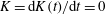 $K=\text{d}K(t)/\text{d}t=0$
into (6.20), and also (1.1), the transient hydrodynamic force for the spherical particle is obtained as
$K=\text{d}K(t)/\text{d}t=0$
into (6.20), and also (1.1), the transient hydrodynamic force for the spherical particle is obtained as
 $$\begin{eqnarray}\displaystyle \boldsymbol{F} & = & \displaystyle \left\{6\unicode[STIX]{x03C0}\unicode[STIX]{x1D707}au_{max}+\frac{2}{3}\unicode[STIX]{x03C0}\unicode[STIX]{x1D70C}a^{3}\frac{\text{d}u_{max}}{\text{d}t}+6\unicode[STIX]{x03C0}\unicode[STIX]{x1D70C}a^{2}\sqrt{\frac{\unicode[STIX]{x1D708}}{\unicode[STIX]{x03C0}}}\int _{0}^{t}\frac{\text{d}u_{max}}{\text{d}\unicode[STIX]{x1D70F}}\frac{1}{\sqrt{t-\unicode[STIX]{x1D70F}}}\,\text{d}\unicode[STIX]{x1D70F}\right.\nonumber\\ \displaystyle & & \displaystyle -\,4\unicode[STIX]{x03C0}\unicode[STIX]{x1D707}au_{max}\left(\frac{a}{R_{0}}\right)^{2}-\frac{4}{15}\unicode[STIX]{x03C0}\unicode[STIX]{x1D70C}a^{3}\left(\frac{a}{R_{0}}\right)^{2}\frac{\text{d}u_{max}}{\text{d}t}\nonumber\\ \displaystyle & & \displaystyle -\,4\unicode[STIX]{x03C0}\unicode[STIX]{x1D70C}a^{2}\sqrt{\frac{\unicode[STIX]{x1D708}}{\unicode[STIX]{x03C0}}}\left(\frac{a}{R_{0}}\right)^{2}\int _{0}^{t}\frac{\text{d}u_{max}}{\text{d}\unicode[STIX]{x1D70F}}\frac{1}{\sqrt{t-\unicode[STIX]{x1D70F}}}\,\text{d}\unicode[STIX]{x1D70F}\nonumber\\ \displaystyle & & \displaystyle -\,\frac{28\sqrt{3}}{45}\unicode[STIX]{x03C0}\unicode[STIX]{x1D70C}a^{2}\sqrt{\frac{\unicode[STIX]{x1D708}}{\unicode[STIX]{x03C0}}}\left(\frac{a}{R_{0}}\right)^{2}\int _{0}^{t}\frac{\text{d}u_{max}}{\text{d}\unicode[STIX]{x1D70F}}S_{F1}(t-\unicode[STIX]{x1D70F})\,\text{d}\unicode[STIX]{x1D70F}\nonumber\\ \displaystyle & & \displaystyle \left.-\,\frac{28\sqrt{3}}{45}\unicode[STIX]{x03C0}\unicode[STIX]{x1D70C}a^{3}\left(\frac{a}{R_{0}}\right)^{2}\int _{0}^{t}\frac{\text{d}^{2}u_{max}}{\text{d}\unicode[STIX]{x1D70F}^{2}}S_{F2}(t-\unicode[STIX]{x1D70F})\,\text{d}\unicode[STIX]{x1D70F}\right\}\boldsymbol{e}_{\boldsymbol{x}}.\end{eqnarray}$$
It should be noted that the force in (6.30) is also an approximated solution, and the corresponding contribution is due to the first reflected flow field. Similarly, it is also asymptotically correct only in the limit of small
 $a/R_{0}\ll 1$
. When the boundary condition of the Poiseuille flow is steady and
$a/R_{0}\ll 1$
. When the boundary condition of the Poiseuille flow is steady and
 $u_{max}(t)=\text{constant}=U_{0}$
, the force in (6.30) agrees with (6.27), as expected.
$u_{max}(t)=\text{constant}=U_{0}$
, the force in (6.30) agrees with (6.27), as expected.
7 Conclusion
In this paper, we have addressed the concept of fundamental solutions of the unsteady singularities in order to describe the behaviour of a sphere in unsteady Stokes flows. The singularity method, characterized by different unsteady singularities, and combinations with the convolution theorem have been used to give an analytical method that is more potent and general than the traditional methods using the Fourier transform. Also more importantly, this proposed method does not need the assumption of rotary or translational oscillation to solve the exact solution of transient force or torque for flow past a sphere. From the demonstrating examples, the convolution equations are finally governed by Volterra integral equations of the first kind. The velocity field can be calculated by numerical inversion of the Laplace transform in terms of the strengths of unsteady singularities in the Laplace domain, such as in the case of axisymmetric parabolic flow past a sphere. The main advantage of this approach is that it requires only the Laplace transform of fundamental solutions instead of the time-domain fundamental solutions of the governing equations. In general we still obtain stable and accurate results. As a consequence most of the steady Stokes solutions can be deduced from this unsteady analysis of Stokes flow problems.
Appendix A. Derivation of the hydrodynamic force due to an unsteady potential dipole
A potential singularity is important in problems of both potential flows as well as Stokes flows. The Helmholtz decomposition theorem, regarded as the fundamental theorem of vector calculus, describes that every vector field
 $\boldsymbol{u}$
can be decomposed as the sum of a rotational part
$\boldsymbol{u}$
can be decomposed as the sum of a rotational part
 $\boldsymbol{v}$
and an irrotational part
$\boldsymbol{v}$
and an irrotational part
 $\unicode[STIX]{x1D735}\unicode[STIX]{x1D719}$
:
$\unicode[STIX]{x1D735}\unicode[STIX]{x1D719}$
:
 $$\begin{eqnarray}\displaystyle \boldsymbol{u}=\unicode[STIX]{x1D735}\unicode[STIX]{x1D719}+\boldsymbol{v}. & & \displaystyle\end{eqnarray}$$
In terms of the rotational and irrotational fields, it is convenient to substitute (A 1) into the unsteady Stokes equations and express the equations decomposed into two parts:
 $$\begin{eqnarray}\displaystyle \left.\begin{array}{@{}c@{}}\unicode[STIX]{x1D735}\boldsymbol{\cdot }\boldsymbol{v}=0\\ \displaystyle \unicode[STIX]{x1D70C}\frac{\unicode[STIX]{x2202}\boldsymbol{v}}{\unicode[STIX]{x2202}t}=-\unicode[STIX]{x1D735}p^{R}+\unicode[STIX]{x1D707}\unicode[STIX]{x1D6FB}^{2}\boldsymbol{v}+\boldsymbol{f}\end{array}\right\},\quad \left.\begin{array}{@{}c@{}}\unicode[STIX]{x1D6FB}^{2}\unicode[STIX]{x1D719}=0\\ \displaystyle \unicode[STIX]{x1D70C}\frac{\unicode[STIX]{x2202}}{\unicode[STIX]{x2202}t}(\unicode[STIX]{x1D735}\unicode[STIX]{x1D719})=-\unicode[STIX]{x1D735}p^{IR}\end{array}\right\}, & & \displaystyle\end{eqnarray}$$
where
 $p^{R}$
,
$p^{R}$
,
 $p^{IR}$
are the induced pressure of rotational and irrotational part, respectively. The potential singularities in (A 2b
) have been widely used in potential flows. For example, the familiar singularities are the point source, doublet (dipole), etc. Next, it is easily discovered that the potential
$p^{IR}$
are the induced pressure of rotational and irrotational part, respectively. The potential singularities in (A 2b
) have been widely used in potential flows. For example, the familiar singularities are the point source, doublet (dipole), etc. Next, it is easily discovered that the potential
 $\unicode[STIX]{x1D719}(t)=-m(t)/4\unicode[STIX]{x03C0}r$
satisfies
$\unicode[STIX]{x1D719}(t)=-m(t)/4\unicode[STIX]{x03C0}r$
satisfies
 $\unicode[STIX]{x1D6FB}^{2}\unicode[STIX]{x1D719}=0$
, in three dimensions, and
$\unicode[STIX]{x1D6FB}^{2}\unicode[STIX]{x1D719}=0$
, in three dimensions, and
 $m(t)$
is related to the mass rate. By taking the gradient of
$m(t)$
is related to the mass rate. By taking the gradient of
 $\unicode[STIX]{x1D719}$
to get velocity and solving (A 2b
) for the pressure, we obtain the velocity and pressure of a point source as
$\unicode[STIX]{x1D719}$
to get velocity and solving (A 2b
) for the pressure, we obtain the velocity and pressure of a point source as
 $$\begin{eqnarray}\displaystyle & \displaystyle u_{i}(\boldsymbol{x},t)=\frac{1}{4\unicode[STIX]{x03C0}}\frac{\hat{x}_{i}}{r^{3}}m(t), & \displaystyle\end{eqnarray}$$
 $$\begin{eqnarray}\displaystyle & \displaystyle p(\boldsymbol{x},t)=\frac{\unicode[STIX]{x1D70C}}{4\unicode[STIX]{x03C0}r}\frac{\text{d}}{\text{d}t}(m(t)). & \displaystyle\end{eqnarray}$$
To differentiate successively the point source with respect to the point
 $\boldsymbol{x}_{\mathbf{0}}$
, we can obtain the higher-order singularities. Thus the induced velocity for an unsteady potential dipole is given by
$\boldsymbol{x}_{\mathbf{0}}$
, we can obtain the higher-order singularities. Thus the induced velocity for an unsteady potential dipole is given by
 $$\begin{eqnarray}\displaystyle u_{i}(\boldsymbol{x},t)=\frac{1}{4\unicode[STIX]{x03C0}}G_{ij}^{PD}(\hat{\boldsymbol{x}})d_{j}(t)=\frac{1}{4\unicode[STIX]{x03C0}}\left(-\frac{\unicode[STIX]{x1D6FF}_{ij}}{r^{3}}+3\frac{\hat{x}_{i}\hat{x}_{j}}{r^{5}}\right)d_{j}(t). & & \displaystyle\end{eqnarray}$$
The induced pressure of an unsteady potential dipole is
 $$\begin{eqnarray}\displaystyle p(\boldsymbol{x},t)=\frac{\unicode[STIX]{x1D70C}}{4\unicode[STIX]{x03C0}}\frac{\hat{x}_{i}}{r^{3}}\frac{\text{d}}{\text{d}t}(d_{i}(t)). & & \displaystyle\end{eqnarray}$$
The surrounding fluid exerts a force on the sphere of radius
 $a$
centered at an unsteady potential dipole. We obtain the force acting on the sphere as
$a$
centered at an unsteady potential dipole. We obtain the force acting on the sphere as
 $$\begin{eqnarray}\displaystyle F_{i}(t)=-\frac{\unicode[STIX]{x1D70C}}{3}\frac{\text{d}}{\text{d}t}(d_{i}(t)). & & \displaystyle\end{eqnarray}$$
Appendix B. Derivations of unsteady strengths of stresslet, rotlet and potential quadrupole in the Laplace transform domain for the case of a shear flow past a sphere
Implementing the boundary condition (
 $u=0$
at
$u=0$
at
 $(x,y,z)=(0,a,0)$
in (B 1),
$(x,y,z)=(0,a,0)$
in (B 1),
 $v=0$
at
$v=0$
at
 $(x,y,z)=(a,0,0)$
in (B 2),
$(x,y,z)=(a,0,0)$
in (B 2),
 $w=0$
at
$w=0$
at
 $r=a$
in (B 3)) to be satisfied and taking the Laplace transform of (4.1), and using the tables of integral transforms (Sneddon Reference Sneddon1972), we obtain three equations for three unknown strengths of the singularities when all
$r=a$
in (B 3)) to be satisfied and taking the Laplace transform of (4.1), and using the tables of integral transforms (Sneddon Reference Sneddon1972), we obtain three equations for three unknown strengths of the singularities when all
 $i,j,k$
each take values 1, 2 and 3 in three dimensions, namely
$i,j,k$
each take values 1, 2 and 3 in three dimensions, namely
 $$\begin{eqnarray}\displaystyle 0 & = & \displaystyle \hat{\dot{\unicode[STIX]{x1D6FE}}}(s)a+\frac{1}{4\unicode[STIX]{x03C0}\unicode[STIX]{x1D70C}}\left(\begin{array}{@{}l@{}}\displaystyle \frac{3}{\sqrt{\unicode[STIX]{x1D708}}a^{3}}\frac{\text{e}^{-\sqrt{a^{2}s/\unicode[STIX]{x1D708}}}}{\sqrt{s}}+\frac{3}{2\unicode[STIX]{x1D708}a^{2}}\text{e}^{-\sqrt{a^{2}s/\unicode[STIX]{x1D708}}}+\frac{1}{2\unicode[STIX]{x1D708}^{3/2}a}\sqrt{s}\text{e}^{-\sqrt{a^{2}s/\unicode[STIX]{x1D708}}}\\ \displaystyle +\,\frac{3}{a^{4}}\left(-\frac{1}{s}+\frac{\text{e}^{-\sqrt{a^{2}s/\unicode[STIX]{x1D708}}}}{s}\right)\end{array}\right){\hat{S}}_{12}(s)\nonumber\\ \displaystyle & & \displaystyle +\,\frac{1}{4\unicode[STIX]{x03C0}\unicode[STIX]{x1D70C}}\left(-\frac{1}{\unicode[STIX]{x1D708}a^{2}}\text{e}^{-\sqrt{a^{2}s/\unicode[STIX]{x1D708}}}-\frac{1}{\unicode[STIX]{x1D708}^{3/2}a}\sqrt{s}\text{e}^{-\sqrt{a^{2}s/\unicode[STIX]{x1D708}}}\right)\hat{\unicode[STIX]{x1D6FA}}_{3}(s)+\frac{1}{4\unicode[STIX]{x03C0}}\left(-\frac{3}{a^{4}}\right)\hat{Q}_{12}(s),\end{eqnarray}$$
 $$\begin{eqnarray}\displaystyle 0 & = & \displaystyle \frac{1}{4\unicode[STIX]{x03C0}\unicode[STIX]{x1D70C}}\left(\begin{array}{@{}l@{}}\displaystyle \frac{3}{\sqrt{\unicode[STIX]{x1D708}}a^{3}}\frac{\text{e}^{-\sqrt{a^{2}s/\unicode[STIX]{x1D708}}}}{\sqrt{s}}+\frac{3}{2\unicode[STIX]{x1D708}a^{2}}\text{e}^{-\sqrt{a^{2}s/\unicode[STIX]{x1D708}}}+\frac{1}{2\unicode[STIX]{x1D708}^{3/2}a}\sqrt{s}\text{e}^{-\sqrt{a^{2}s/\unicode[STIX]{x1D708}}}\\ \displaystyle +\,\frac{3}{a^{4}}\left(\frac{-1}{s}+\frac{\text{e}^{-\sqrt{a^{2}s/\unicode[STIX]{x1D708}}}}{s}\right)\end{array}\right){\hat{S}}_{12}(s)\nonumber\\ \displaystyle & & \displaystyle +\,\frac{1}{4\unicode[STIX]{x03C0}\unicode[STIX]{x1D70C}}\left(\!\frac{1}{\unicode[STIX]{x1D708}a^{2}}\text{e}^{-\sqrt{a^{2}s/\unicode[STIX]{x1D708}}}+\frac{1}{\unicode[STIX]{x1D708}^{3/2}a}\sqrt{s}\text{e}^{-\sqrt{a^{2}s/\unicode[STIX]{x1D708}}}\right)\hat{\unicode[STIX]{x1D6FA}}_{3}(s)\!+\frac{1}{4\unicode[STIX]{x03C0}}\left(\!-\frac{3}{a^{4}}\right)\hat{Q}_{12}(s),\end{eqnarray}$$
 $$\begin{eqnarray}\displaystyle 0 & = & \displaystyle \frac{1}{4\unicode[STIX]{x03C0}\unicode[STIX]{x1D70C}}\left(\begin{array}{@{}l@{}}\displaystyle -\frac{15}{\sqrt{\unicode[STIX]{x1D708}}a^{3}}\frac{\text{e}^{-\sqrt{a^{2}s/\unicode[STIX]{x1D708}}}}{\sqrt{s}}-\frac{6}{\unicode[STIX]{x1D708}a^{2}}\text{e}^{-\sqrt{a^{2}s/\unicode[STIX]{x1D708}}}-\frac{1}{\unicode[STIX]{x1D708}^{3/2}a}\sqrt{s}\text{e}^{-\sqrt{a^{2}s/\unicode[STIX]{x1D708}}}\\ \displaystyle +\,\frac{15}{a^{4}}\left(\frac{1}{s}-\frac{\text{e}^{-\sqrt{a^{2}s/\unicode[STIX]{x1D708}}}}{s}\right)\end{array}\right){\hat{S}}_{12}(s)\nonumber\\ \displaystyle & & \displaystyle +\,\frac{1}{4\unicode[STIX]{x03C0}}\left(\frac{15}{a^{4}}\right)\hat{Q}_{12}(s).\end{eqnarray}$$
From (B 1) to (B 3), the unsteady strengths of stresslet, rotlet and potential quadrupole in the Laplace transform domain can then be computed to be (4.3) to (4.5).
Appendix C. Derivation of the coefficients of the singularities for axisymmetric parabolic flow past a sphere
Implementing the boundary condition (
 $u=0$
at
$u=0$
at
 $(x,y,z)=(0,a,0)$
in (C 1),
$(x,y,z)=(0,a,0)$
in (C 1),
 $u=0$
at
$u=0$
at
 $(x,y,z)=(a,0,0)$
in (C 2),
$(x,y,z)=(a,0,0)$
in (C 2),
 $v=0$
at
$v=0$
at
 $r=a$
in (C 3), (C 4)) to be satisfied and taking the Laplace transform of (6.1), and using the tables of integral transforms (Sneddon Reference Sneddon1972), we obtain four equations for four unknown strengths of the singularities when all
$r=a$
in (C 3), (C 4)) to be satisfied and taking the Laplace transform of (6.1), and using the tables of integral transforms (Sneddon Reference Sneddon1972), we obtain four equations for four unknown strengths of the singularities when all
 $i,j,k,l$
each take values 1, 2 and 3 in three dimensions, namely
$i,j,k,l$
each take values 1, 2 and 3 in three dimensions, namely
 $$\begin{eqnarray}\displaystyle 0 & = & \displaystyle K(s)a^{2}+\frac{1}{4\unicode[STIX]{x03C0}\unicode[STIX]{x1D70C}}\left(\frac{1}{\sqrt{\unicode[STIX]{x1D708}}a^{2}}\frac{\text{e}^{-\sqrt{a^{2}s/\unicode[STIX]{x1D708}}}}{\sqrt{s}}+\frac{1}{\unicode[STIX]{x1D708}a}\text{e}^{-\sqrt{a^{2}s/\unicode[STIX]{x1D708}}}-\frac{1}{a^{3}}\left(\frac{1}{s}-\frac{\text{e}^{-\sqrt{a^{2}s/\unicode[STIX]{x1D708}}}}{s}\right)\right)\hat{\unicode[STIX]{x1D6FC}}_{1}(s)\nonumber\\ \displaystyle & & \displaystyle +\,\frac{1}{4\unicode[STIX]{x03C0}}\left(-\frac{1}{a^{3}}\right)\hat{d}_{1}(s)\nonumber\\ \displaystyle & & \displaystyle +\,\frac{1}{4\unicode[STIX]{x03C0}\unicode[STIX]{x1D70C}}\left(\begin{array}{@{}l@{}}\displaystyle -\frac{9}{\sqrt{\unicode[STIX]{x1D708}}a^{4}}\frac{\text{e}^{-\sqrt{a^{2}s/\unicode[STIX]{x1D708}}}}{\sqrt{s}}-\frac{4}{\unicode[STIX]{x1D708}a^{3}}\text{e}^{-\sqrt{a^{2}s/\unicode[STIX]{x1D708}}}-\frac{1}{\unicode[STIX]{x1D708}^{3/2}a^{2}}\sqrt{s}\text{e}^{-\sqrt{a^{2}s/\unicode[STIX]{x1D708}}}\\ \displaystyle +\,\frac{9}{a^{5}}\left(\frac{1}{s}-\frac{\text{e}^{-\sqrt{a^{2}s/\unicode[STIX]{x1D708}}}}{s}\right)\end{array}\right)\hat{Q}_{111}(s)\nonumber\\ \displaystyle & & \displaystyle +\,\frac{1}{4\unicode[STIX]{x03C0}}\left(\frac{9}{a^{5}}\right)\hat{O} _{111}(s),\end{eqnarray}$$
 $$\begin{eqnarray}\displaystyle 0 & = & \displaystyle \frac{1}{4\unicode[STIX]{x03C0}\unicode[STIX]{x1D70C}}\left(-\frac{2}{\sqrt{\unicode[STIX]{x1D708}}a^{2}}\frac{\text{e}^{-\sqrt{a^{2}s/\unicode[STIX]{x1D708}}}}{\sqrt{s}}+\frac{2}{a^{3}}\left(\frac{1}{s}-\frac{\text{e}^{-\sqrt{a^{2}s/\unicode[STIX]{x1D708}}}}{s}\right)\right)\hat{\unicode[STIX]{x1D6FC}}_{1}(s)+\frac{1}{4\unicode[STIX]{x03C0}}\left(\frac{2}{a^{3}}\right)\hat{d}_{1}(s)\nonumber\\ \displaystyle & & \displaystyle +\,\frac{1}{4\unicode[STIX]{x03C0}\unicode[STIX]{x1D70C}}\left(\begin{array}{@{}l@{}}\displaystyle -\frac{24}{\sqrt{\unicode[STIX]{x1D708}}a^{4}}\frac{\text{e}^{-\sqrt{a^{2}s/\unicode[STIX]{x1D708}}}}{\sqrt{s}}-\frac{10}{\unicode[STIX]{x1D708}a^{3}}\text{e}^{-\sqrt{a^{2}s/\unicode[STIX]{x1D708}}}-\frac{2}{\unicode[STIX]{x1D708}^{3/2}a^{2}}\sqrt{s}\text{e}^{-\sqrt{a^{2}s/\unicode[STIX]{x1D708}}}\\ \displaystyle +\,\frac{24}{a^{5}}\left(\frac{1}{s}-\frac{\text{e}^{-\sqrt{a^{2}s/\unicode[STIX]{x1D708}}}}{s}\right)\end{array}\right)\hat{Q}_{111}(s)\nonumber\\ \displaystyle & & \displaystyle +\,\frac{1}{4\unicode[STIX]{x03C0}}\left(\frac{24}{a^{5}}\right)\hat{O} _{111}(s),\end{eqnarray}$$
 $$\begin{eqnarray}\displaystyle 0 & = & \displaystyle \frac{1}{4\unicode[STIX]{x03C0}\unicode[STIX]{x1D70C}}\left(-\frac{3}{\sqrt{\unicode[STIX]{x1D708}}a^{2}}\frac{\text{e}^{-\sqrt{a^{2}s/\unicode[STIX]{x1D708}}}}{\sqrt{s}}-\frac{1}{\unicode[STIX]{x1D708}a}\text{e}^{-\sqrt{a^{2}s/\unicode[STIX]{x1D708}}}+\frac{3}{a^{3}}\left(\frac{1}{s}-\frac{\text{e}^{-\sqrt{a^{2}s/\unicode[STIX]{x1D708}}}}{s}\right)\right)\hat{\unicode[STIX]{x1D6FC}}_{1}(s)\nonumber\\ \displaystyle & & \displaystyle +\,\frac{1}{4\unicode[STIX]{x03C0}}\left(\frac{3}{a^{3}}\right)\hat{d}_{1}(s)\nonumber\\ \displaystyle & & \displaystyle +\,\frac{1}{4\unicode[STIX]{x03C0}\unicode[STIX]{x1D70C}}\left(\begin{array}{@{}l@{}}\displaystyle \frac{45}{\sqrt{\unicode[STIX]{x1D708}}a^{4}}\frac{\text{e}^{-\sqrt{a^{2}s/\unicode[STIX]{x1D708}}}}{\sqrt{s}}+\frac{18}{\unicode[STIX]{x1D708}a^{3}}\text{e}^{-\sqrt{a^{2}s/\unicode[STIX]{x1D708}}}+\frac{3}{\unicode[STIX]{x1D708}^{3/2}a^{2}}\sqrt{s}\text{e}^{-\sqrt{a^{2}s/\unicode[STIX]{x1D708}}}\\ \displaystyle -\,\frac{45}{a^{5}}\left(\frac{1}{s}-\frac{\text{e}^{-\sqrt{a^{2}s/\unicode[STIX]{x1D708}}}}{s}\right)\end{array}\right)\hat{Q}_{111}(s)\nonumber\\ \displaystyle & & \displaystyle +\,\frac{1}{4\unicode[STIX]{x03C0}}\left(-\frac{45}{a^{5}}\right)\hat{O} _{111}(s),\end{eqnarray}$$
 $$\begin{eqnarray}\displaystyle 0 & = & \displaystyle \frac{1}{4\unicode[STIX]{x03C0}\unicode[STIX]{x1D70C}}\left(\begin{array}{@{}l@{}}\displaystyle -\frac{105}{\sqrt{\unicode[STIX]{x1D708}}a^{4}}\frac{\text{e}^{-\sqrt{a^{2}s/\unicode[STIX]{x1D708}}}}{\sqrt{s}}-\frac{45}{\unicode[STIX]{x1D708}a^{3}}\text{e}^{-\sqrt{a^{2}s/\unicode[STIX]{x1D708}}}-\frac{10}{\unicode[STIX]{x1D708}^{3/2}a^{2}}\sqrt{s}\text{e}^{-\sqrt{a^{2}s/\unicode[STIX]{x1D708}}}\\ \displaystyle -\,\frac{1}{\unicode[STIX]{x1D708}^{2}a}s\text{e}^{-\sqrt{a^{2}s/\unicode[STIX]{x1D708}}}+\frac{105}{a^{5}}\left(\frac{1}{s}-\frac{\text{e}^{-\sqrt{a^{2}s/\unicode[STIX]{x1D708}}}}{s}\right)\end{array}\right)\hat{Q}_{111}(s)\nonumber\\ \displaystyle & & \displaystyle +\,\frac{1}{4\unicode[STIX]{x03C0}}\left(\frac{105}{a^{5}}\right)\hat{O} _{111}(s).\end{eqnarray}$$
Solving the system, we obtain unknown strengths of
 $\hat{\unicode[STIX]{x1D6FC}}_{1}(s),\hat{d}_{1}(s),\hat{Q}_{111}(s)$
and
$\hat{\unicode[STIX]{x1D6FC}}_{1}(s),\hat{d}_{1}(s),\hat{Q}_{111}(s)$
and
 $\hat{O} _{111}(s)$
in the Laplace domain as given by (6.3)–(6.6).
$\hat{O} _{111}(s)$
in the Laplace domain as given by (6.3)–(6.6).
Appendix D. Derivation of the hydrodynamic force due to an unsteady Stokeslet
The viscous force due to an unsteady Stokeslet in the Laplace domain is
 $$\begin{eqnarray}\displaystyle \boldsymbol{F}_{\boldsymbol{s},\boldsymbol{v}}(s)=\left\{\frac{8}{3}\unicode[STIX]{x03C0}\unicode[STIX]{x1D707}a^{3}K(s)+\frac{8}{3}\unicode[STIX]{x03C0}\unicode[STIX]{x1D70C}a^{4}\sqrt{\unicode[STIX]{x1D708}}\sqrt{s}K(s)+\frac{14}{45}\unicode[STIX]{x03C0}\unicode[STIX]{x1D70C}a^{5}\frac{s\left(1+\displaystyle \frac{a}{\sqrt{\unicode[STIX]{x1D708}}}\sqrt{s}\right)}{1+\displaystyle \frac{a}{\sqrt{\unicode[STIX]{x1D708}}}\sqrt{s}+\frac{a^{2}}{3\unicode[STIX]{x1D708}}s}K(s)\right\}\boldsymbol{e}_{\boldsymbol{x}}. & & \displaystyle \nonumber\\ \displaystyle & & \displaystyle\end{eqnarray}$$
Taking the inverse Laplace transform, the first and second term give
 $$\begin{eqnarray}\displaystyle \left.\begin{array}{@{}c@{}}\displaystyle \mathscr{L}^{-1}\left({\textstyle \frac{8}{3}}\unicode[STIX]{x03C0}\unicode[STIX]{x1D707}a^{3}K(s)\right)={\textstyle \frac{8}{3}}\unicode[STIX]{x03C0}\unicode[STIX]{x1D707}a^{3}K(t),\\ \displaystyle \mathscr{L}^{-1}\left(\frac{8}{3}\unicode[STIX]{x03C0}\unicode[STIX]{x1D70C}a^{4}\sqrt{\unicode[STIX]{x1D708}}\sqrt{s}K(s)\right)=\frac{8}{3}\unicode[STIX]{x03C0}\unicode[STIX]{x1D70C}a^{4}\sqrt{\frac{\unicode[STIX]{x1D708}}{\unicode[STIX]{x03C0}}}\int _{0}^{t}\frac{\text{d}K}{\text{d}\unicode[STIX]{x1D70F}}\frac{1}{\sqrt{t-\unicode[STIX]{x1D70F}}}\,\text{d}\unicode[STIX]{x1D70F}+\frac{8}{3}\unicode[STIX]{x03C0}\unicode[STIX]{x1D70C}a^{4}\sqrt{\frac{\unicode[STIX]{x1D708}}{\unicode[STIX]{x03C0}}}K(0)\frac{1}{\sqrt{t}}.\end{array}\right\} & & \displaystyle \nonumber\\ \displaystyle & & \displaystyle\end{eqnarray}$$
The third term on the right-hand side can be divided into two terms:
 $$\begin{eqnarray}\displaystyle & & \displaystyle \frac{14}{45}\unicode[STIX]{x03C0}\unicode[STIX]{x1D70C}a^{5}\frac{s\left(1+\displaystyle \frac{a}{\sqrt{\unicode[STIX]{x1D708}}}\sqrt{s}\right)}{1+\displaystyle \frac{a}{\sqrt{\unicode[STIX]{x1D708}}}\sqrt{s}+\frac{a^{2}}{3\unicode[STIX]{x1D708}}s}K(s)\nonumber\\ \displaystyle & & \displaystyle \quad =\frac{14}{45}\unicode[STIX]{x03C0}\unicode[STIX]{x1D70C}a^{5}\frac{sK(s)}{1+\displaystyle \frac{a}{\sqrt{\unicode[STIX]{x1D708}}}\sqrt{s}+\frac{a^{2}}{3\unicode[STIX]{x1D708}}s}+\frac{14}{45}\unicode[STIX]{x03C0}\unicode[STIX]{x1D70C}a^{5}\frac{\displaystyle \frac{a}{\sqrt{\unicode[STIX]{x1D708}}}s^{2}K(s)}{\sqrt{s}\left(1+\displaystyle \frac{a}{\sqrt{\unicode[STIX]{x1D708}}}\sqrt{s}+\frac{a^{2}}{3\unicode[STIX]{x1D708}}s\right)}.\end{eqnarray}$$
Next, using the tables of integral transforms (Sneddon Reference Sneddon1972),
 $$\begin{eqnarray}\displaystyle \mathscr{L}(\text{e}^{c^{2}t}\text{erfc}(c\sqrt{t}))=\frac{1}{\sqrt{s}(\sqrt{s}+c)};\quad \mathscr{L}\left(\frac{1}{\sqrt{\unicode[STIX]{x03C0}t}}-c\text{e}^{c^{2}t}\text{erfc}(c\sqrt{t})\right)=\frac{1}{\sqrt{s}+c}. & & \displaystyle \nonumber\\ \displaystyle & & \displaystyle\end{eqnarray}$$
And the inverse Laplace transform with the first term partly on the right-hand side in (D 3) is
 $$\begin{eqnarray}\displaystyle & & \displaystyle \mathscr{L}^{-1}\left(\frac{1}{1+\displaystyle \frac{a}{\sqrt{\unicode[STIX]{x1D708}}}\sqrt{s}+\frac{a^{2}}{3\unicode[STIX]{x1D708}}s}\right)=\frac{3\sqrt{\unicode[STIX]{x1D708}}}{a}\frac{1}{\sqrt{3}i}\mathscr{L}^{-1}\left(\frac{1}{\displaystyle \sqrt{s}+\frac{\sqrt{\unicode[STIX]{x1D708}}}{a}\hat{\unicode[STIX]{x1D6FD}}}-\frac{1}{\displaystyle \sqrt{s}+\frac{\sqrt{\unicode[STIX]{x1D708}}}{a}\unicode[STIX]{x1D6FD}}\right)\nonumber\\ \displaystyle & & \displaystyle \quad =\frac{3\sqrt{\unicode[STIX]{x1D708}}}{a}\frac{1}{\sqrt{3}\text{i}}\!\left(\left(\frac{\sqrt{\unicode[STIX]{x1D708}}}{a}\unicode[STIX]{x1D6FD}\right)\text{e}^{(\unicode[STIX]{x1D708}/a^{2})\unicode[STIX]{x1D6FD}^{2}t}\text{erfc}\left(\frac{\sqrt{\unicode[STIX]{x1D708}}}{a}\unicode[STIX]{x1D6FD}\sqrt{t}\right)-\left(\frac{\sqrt{\unicode[STIX]{x1D708}}}{a}\hat{\unicode[STIX]{x1D6FD}}\right)\text{e}^{(\unicode[STIX]{x1D708}/a^{2})\hat{\unicode[STIX]{x1D6FD}}^{2}t}\text{erfc}\left(\frac{\sqrt{\unicode[STIX]{x1D708}}}{a}\hat{\unicode[STIX]{x1D6FD}}\sqrt{t}\right)\!\right)\nonumber\\ \displaystyle & & \displaystyle \quad =\frac{\sqrt{\unicode[STIX]{x1D708}}}{a}2\sqrt{3}\left(\text{Im}\left(\left(\frac{\sqrt{\unicode[STIX]{x1D708}}}{a}\unicode[STIX]{x1D6FD}\right)\text{e}^{(\unicode[STIX]{x1D707}/a^{2})\unicode[STIX]{x1D6FD}^{2}t}\text{erfc}\left(\frac{\sqrt{\unicode[STIX]{x1D708}}}{a}\unicode[STIX]{x1D6FD}\sqrt{t}\right)\right)\right)\nonumber\\ \displaystyle & & \displaystyle \quad \text{and}~\unicode[STIX]{x1D6FD}=\frac{3}{2}+\frac{\sqrt{3}}{2}\text{i};\quad \hat{\unicode[STIX]{x1D6FD}}=\frac{3}{2}-\frac{\sqrt{3}}{2}\text{i}.\end{eqnarray}$$
The inverse Laplace transform with the second term partly on the right-hand side in (D 3) is
 $$\begin{eqnarray}\displaystyle & & \displaystyle \mathscr{L}^{-1}\left(\frac{\displaystyle \frac{a}{\sqrt{\unicode[STIX]{x1D708}}}}{\sqrt{s}\left(1+\displaystyle \frac{a}{\sqrt{\unicode[STIX]{x1D708}}}\sqrt{s}+\frac{a^{2}}{3\unicode[STIX]{x1D708}}s\right)}\right)\nonumber\\ \displaystyle & & \displaystyle \quad =\frac{\sqrt{3}}{\text{i}}\mathscr{L}^{-1}\left(\frac{1}{\sqrt{s}\left(\sqrt{s}+\displaystyle \frac{\sqrt{\unicode[STIX]{x1D708}}}{a}\hat{\unicode[STIX]{x1D6FD}}\right)}-\frac{1}{\sqrt{s}\left(\sqrt{s}+\displaystyle \frac{\sqrt{\unicode[STIX]{x1D708}}}{a}\unicode[STIX]{x1D6FD}\right)}\right)\nonumber\\ \displaystyle & & \displaystyle \quad =\frac{\sqrt{3}}{\text{i}}\left(\text{e}^{(\unicode[STIX]{x1D708}/a^{2})\hat{\unicode[STIX]{x1D6FD}}^{2}t}\text{erfc}\left(\frac{\sqrt{\unicode[STIX]{x1D708}}}{a}\hat{\unicode[STIX]{x1D6FD}}\sqrt{t}\right)-\text{e}^{(\unicode[STIX]{x1D708}/a^{2})\unicode[STIX]{x1D6FD}^{2}t}\text{erfc}\left(\frac{\sqrt{\unicode[STIX]{x1D708}}}{a}\unicode[STIX]{x1D6FD}\sqrt{t}\right)\right)\nonumber\\ \displaystyle & & \displaystyle \quad =-2\sqrt{3}\left(\text{Im}\left(\text{e}^{(\unicode[STIX]{x1D708}/a^{2})\unicode[STIX]{x1D6FD}^{2}t}\text{erfc}\left(\frac{\sqrt{\unicode[STIX]{x1D708}}}{a}\unicode[STIX]{x1D6FD}\sqrt{t}\right)\right)\right).\end{eqnarray}$$
Making use of (D 5) and the convolution theorem, the first term on the right-hand side in (D 3) is
 $$\begin{eqnarray}\displaystyle & & \displaystyle \mathscr{L}^{-1}\left(\frac{14}{45}\unicode[STIX]{x03C0}\unicode[STIX]{x1D70C}a^{5}\frac{sK(s)}{1+\displaystyle \frac{a}{\sqrt{\unicode[STIX]{x1D708}}}\sqrt{s}+\frac{a^{2}}{3\unicode[STIX]{x1D708}}s}\right)\nonumber\\ \displaystyle & & \displaystyle \quad =\frac{28\sqrt{3}}{45}\unicode[STIX]{x03C0}\unicode[STIX]{x1D70C}a^{4}\sqrt{\frac{\unicode[STIX]{x1D708}}{\unicode[STIX]{x03C0}}}\int _{0}^{t}\frac{\text{d}K}{\text{d}\unicode[STIX]{x1D70F}}S_{F1}(t-\unicode[STIX]{x1D70F})\,\text{d}\unicode[STIX]{x1D70F}+\frac{28\sqrt{3}}{45}\unicode[STIX]{x03C0}\unicode[STIX]{x1D70C}a^{4}\sqrt{\frac{\unicode[STIX]{x1D708}}{\unicode[STIX]{x03C0}}}K(0)S_{F1}(t),\nonumber\\ \displaystyle & & \displaystyle \quad S_{F1}(t)=\text{Im}\left(\sqrt{\unicode[STIX]{x03C0}}\left(\frac{\sqrt{\unicode[STIX]{x1D708}}\unicode[STIX]{x1D6FD}}{a}\right)\text{e}^{(\unicode[STIX]{x1D708}/a^{2})\unicode[STIX]{x1D6FD}^{2}t}\text{erfc}\left(\frac{\sqrt{\unicode[STIX]{x1D708}}\unicode[STIX]{x1D6FD}}{a}\sqrt{t}\right)\right).\end{eqnarray}$$
In a similar way, using (D 6) and the convolution theorem, the second term on the right-hand side in (D 3) is
 $$\begin{eqnarray}\displaystyle & & \displaystyle \mathscr{L}^{-1}\left(\frac{14}{45}\unicode[STIX]{x03C0}\unicode[STIX]{x1D70C}a^{5}\frac{\displaystyle \frac{a}{\sqrt{\unicode[STIX]{x1D708}}}s^{2}K(s)}{\sqrt{s}\left(1+\displaystyle \frac{a}{\sqrt{\unicode[STIX]{x1D708}}}\sqrt{s}+\frac{a^{2}}{3\unicode[STIX]{x1D708}}s\right)}\right)\nonumber\\ \displaystyle & & \displaystyle \quad =\frac{28\sqrt{3}}{45}\unicode[STIX]{x03C0}\unicode[STIX]{x1D70C}a^{5}\int _{0}^{t}\frac{\text{d}^{2}K}{\text{d}\unicode[STIX]{x1D70F}^{2}}S_{F2}(t-\unicode[STIX]{x1D70F})\,\text{d}\unicode[STIX]{x1D70F}\nonumber\\ \displaystyle & & \displaystyle \qquad +\,\frac{28\sqrt{3}}{45}\unicode[STIX]{x03C0}\unicode[STIX]{x1D70C}a^{5}\left(K(0)\frac{\text{d}}{\text{d}t}(S_{F2}(t))+\left.\frac{\text{d}K}{\text{d}t}\right|_{t=0}S_{F2}(t)\right),\nonumber\\ \displaystyle & & \displaystyle \quad S_{F2}(t)=-\text{Im}\left(\text{e}^{(\unicode[STIX]{x1D708}/a^{2})\unicode[STIX]{x1D6FD}^{2}t}\text{erfc}\left(\frac{\sqrt{\unicode[STIX]{x1D708}}\unicode[STIX]{x1D6FD}}{a}\sqrt{t}\right)\right).\end{eqnarray}$$
Applying (D 2), (D 7) and (D 8), the inverse Laplace transform of
 $\boldsymbol{F}_{\boldsymbol{s},\boldsymbol{v}}(s)$
is
$\boldsymbol{F}_{\boldsymbol{s},\boldsymbol{v}}(s)$
is
 $$\begin{eqnarray}\displaystyle \boldsymbol{F}_{\boldsymbol{s},\boldsymbol{v}}(t) & = & \displaystyle \left\{\frac{8}{3}\unicode[STIX]{x03C0}\unicode[STIX]{x1D707}a^{3}K(t)+\frac{8}{3}\unicode[STIX]{x03C0}\unicode[STIX]{x1D70C}a^{4}\sqrt{\frac{\unicode[STIX]{x1D708}}{\unicode[STIX]{x03C0}}}\int _{0}^{t}\frac{\text{d}K}{\text{d}\unicode[STIX]{x1D70F}}\frac{1}{\sqrt{t-\unicode[STIX]{x1D70F}}}\,\text{d}\unicode[STIX]{x1D70F}\right.\nonumber\\ \displaystyle & & \displaystyle +\,\frac{28\sqrt{3}}{45}\unicode[STIX]{x03C0}\unicode[STIX]{x1D70C}a^{4}\sqrt{\frac{\unicode[STIX]{x1D708}}{\unicode[STIX]{x03C0}}}\int _{0}^{t}\frac{\text{d}K}{\text{d}\unicode[STIX]{x1D70F}}S_{F1}(t-\unicode[STIX]{x1D70F})\,\text{d}\unicode[STIX]{x1D70F}\nonumber\\ \displaystyle & & \displaystyle +\,\frac{28\sqrt{3}}{45}\unicode[STIX]{x03C0}\unicode[STIX]{x1D70C}a^{5}\int _{0}^{t}\frac{\text{d}^{2}K}{\text{d}\unicode[STIX]{x1D70F}^{2}}S_{F2}(t-\unicode[STIX]{x1D70F})\,\text{d}\unicode[STIX]{x1D70F}\nonumber\\ \displaystyle & & \displaystyle +\,\frac{8}{3}\unicode[STIX]{x03C0}\unicode[STIX]{x1D70C}a^{4}\sqrt{\frac{\unicode[STIX]{x1D708}}{\unicode[STIX]{x03C0}}}K(0)\frac{1}{\sqrt{t}}+\frac{28\sqrt{3}}{45}\unicode[STIX]{x03C0}\unicode[STIX]{x1D70C}a^{4}\sqrt{\frac{\unicode[STIX]{x1D708}}{\unicode[STIX]{x03C0}}}K(0)S_{F1}(t)\nonumber\\ \displaystyle & & \displaystyle \left.+\,\frac{28\sqrt{3}}{45}\unicode[STIX]{x03C0}\unicode[STIX]{x1D70C}a^{5}\left(K(0)\frac{\text{d}}{\text{d}t}(S_{F2}(t))+\left.\frac{\text{d}K}{\text{d}t}\right|_{t=0}S_{F2}(t)\right)\right\}\boldsymbol{e}_{\boldsymbol{x}}.\end{eqnarray}$$


