


1. Introduction
Granular gas is a widely used model for describing fluidised granular flows (Goldhirsch Reference Goldhirsch2003). On the microscopic level, it assumes that the grains undergo binary, instantaneous and inelastic collisions (Campbell Reference Campbell1990; Goldhirsch Reference Goldhirsch2003). Similar to molecular gas, the macroscopic description of granular gas can be obtained by dividing the microscopic motion of grains into streaming and fluctuating components, with the former represented by the bulk velocity and the latter by the granular temperature (Campbell Reference Campbell1990; Goldhirsch Reference Goldhirsch2008). This results in compressible hydrodynamic field equations with additional sink terms accounting for the dissipation of granular temperature due to inelastic collisions. In order to complete the hydrodynamic description to the Euler order, equations of state relating density, granular temperature and pressure have been proposed for different regimes of dilute or dense flows (Jenkins & Richman Reference Jenkins and Richman1985; Goldshtein & Shapiro Reference Goldshtein and Shapiro1995; Sirmas et al. Reference Sirmas, Tudorache, Barahona and Radulescu2012; Sirmas & Radulescu Reference Sirmas and Radulescu2019). Additional constitutive relations describing the diffusive effects have been derived from the kinetic theory of granular flow (Jenkins & Richman Reference Jenkins and Richman1985; Campbell Reference Campbell2006) to obtain the Navier–Stokes-order equations.
Compared to molecular gas, the flow of granular gas can become supersonic even under more relaxed flow conditions – for example, as a result of self-organised dynamics during its uniform cooling (Esipov & Pöschel Reference Esipov and Pöschel1997) and gravitational sedimentation (Almazán et al. Reference Almazán, Serero, Salueña and Pöschel2015, Reference Almazán, Serero, Salueña and Pöschel2017) – because its granular temperature is often smaller than its bulk velocity (Tan & Goldhirsch Reference Tan and Goldhirsch1998; Goldshtein, Alexeev & Shapiro Reference Goldshtein, Alexeev and Shapiro2003), which could result in the formation of shock and expansion (Goldshtein, Shapiro & Gutfinger Reference Goldshtein, Shapiro and Gutfinger1996b; Goldshtein et al. Reference Goldshtein, Kamenetsky, Potapov, Shapiro, Campbell and Degani2002) waves. Shock waves in fluidised granular flows have been noticed in canonical compressible flow configurations using both molecular dynamics (Rericha et al. Reference Rericha, Bizon, Shattuck and Swinney2001; Padgett, Mazzoleni & Faw Reference Padgett, Mazzoleni and Faw2015; Sirmas & Radulescu Reference Sirmas and Radulescu2015) and hydrodynamic (Matveev Reference Matveev1983; Goldshtein, Shapiro & Gutfinger Reference Goldshtein, Shapiro and Gutfinger1996a; Kamenetsky et al. Reference Kamenetsky, Goldshtein, Shapiro and Degani2000; Rericha et al. Reference Rericha, Bizon, Shattuck and Swinney2001; Sirmas & Radulescu Reference Sirmas and Radulescu2019) simulations, as well as experiments (Rericha et al. Reference Rericha, Bizon, Shattuck and Swinney2001; Heil et al. Reference Heil, Rericha, Goldman and Swinney2004; Khan et al. Reference Khan, Verma, Hankare, Kumar and Kumar2020), in both one-dimensional (Matveev Reference Matveev1983; Goldshtein et al. Reference Goldshtein, Shapiro and Gutfinger1996a; Kamenetsky et al. Reference Kamenetsky, Goldshtein, Shapiro and Degani2000; Sirmas & Radulescu Reference Sirmas and Radulescu2015, Reference Sirmas and Radulescu2019) and two-dimensional (Rericha et al. Reference Rericha, Bizon, Shattuck and Swinney2001; Wassgren et al. Reference Wassgren, Cordova, Zenit and Karion2003; Heil et al. Reference Heil, Rericha, Goldman and Swinney2004; Soleymani, Zamankhan & Polashenski Reference Soleymani, Zamankhan and Polashenski2004; Padgett et al. Reference Padgett, Mazzoleni and Faw2015; Khan et al. Reference Khan, Verma, Hankare, Kumar and Kumar2020) flows. A shock wave appears in the Euler-order hydrodynamic simulations as a line with zero thickness where the flow variables jump (Kamenetsky et al. Reference Kamenetsky, Goldshtein, Shapiro and Degani2000; Sirmas & Radulescu Reference Sirmas and Radulescu2019). However, a shock layer with small but non-zero thickness appears by including the diffusive effects in the Navier–Stokes-order description (Reddy & Alam Reference Reddy and Alam2015).
A simple one-dimensional flow configuration that has been used to generate planar shock waves is the steady piston motion in a quiescent granular gas (Goldshtein et al. Reference Goldshtein, Shapiro and Gutfinger1996a; Kamenetsky et al. Reference Kamenetsky, Goldshtein, Shapiro and Degani2000; Sirmas & Radulescu Reference Sirmas and Radulescu2015, Reference Sirmas and Radulescu2019). In the moving-piston frame of reference, this problem is identical to a granular gas colliding with a fixed wall, a configuration that was studied by Matveev (Reference Matveev1983) assuming zero granular temperature for the oncoming flow in front of the shock and steady-state conditions. Similar to molecular gas, the jump relations across the shock showed that both pressure and density increase while the absolute velocity decreases. In the region behind the shock, the analytical solution showed that both pressure and density increase monotonically whereas the absolute velocity decreases to become zero at the wall. Matveev (Reference Matveev1983) allowed the density behind the shock to become infinite at the wall because the used equation of state does not take into account the volumetric effects due to the size of the particles. This shortcoming was later avoided in a study of the moving-piston problem where Goldshtein et al. (Reference Goldshtein, Shapiro and Gutfinger1996a) divided the region behind the shock into a fluidised region and a solid block (stagnant layer) region. The steady-state analytical solutions of Goldshtein et al. (Reference Goldshtein, Shapiro and Gutfinger1996a) showed that the behaviour of the fluidised region is similar to that observed by Matveev (Reference Matveev1983). The solid region, however, has almost constant spatial profiles of temperature, velocity and density, whereby the density is equal to that of maximum packing. In subsequent studies (Kamenetsky et al. Reference Kamenetsky, Goldshtein, Shapiro and Degani2000; Sirmas & Radulescu Reference Sirmas and Radulescu2019), time-dependent solutions were obtained by solving the Euler equations numerically, employing a dense granular gas equation of state, which confirmed the existence of these two regions – fluidised region and solid block. Furthermore, it was shown that the shock attains a steady speed after a long evolution time, where the shock strength decreases, confirming the argument of both Matveev (Reference Matveev1983) and Goldshtein et al. (Reference Goldshtein, Shapiro and Gutfinger1996a). A slightly different problem, though its solution has similar features to the piston problem, is the wall collision of granular gas falling under the action of gravity (Pareschi & Russo Reference Pareschi and Russo2005; Serna & Marquina Reference Serna and Marquina2005; Kamath & Du Reference Kamath and Du2009; Aursand et al. Reference Aursand, Evje, Flåtten, Giljarhus and Munkejord2014).
A more general flow configuration, which can generate planar shock waves in addition to other elementary waves such as rarefactions and contact discontinuities, is the Riemann problem. In hyperbolic systems of conservation laws such as the one-dimensional Euler equations for molecular gas, the Riemann problem is an initial value problem with initial data structure consisting of two constant left and right states separated by a discontinuity (LeVeque Reference LeVeque2002; Toro Reference Toro2013). Its solution consists of three elementary waves whose types depend on the values of the initial jump condition in the three primitive variables: density, velocity and pressure. The middle wave is always a contact discontinuity, and the two outer waves are either shocks or rarefactions. The solutions for shock–contact–shock (SCS) wave structure consist of four constant regions separated by these three discontinuities. For dense granular gas, numerical solutions of the Riemann problem include a study by Serna & Marquina (Reference Serna and Marquina2007) using a previously developed shock-capturing scheme (Serna & Marquina Reference Serna and Marquina2005). The initial left state of Serna & Marquina (Reference Serna and Marquina2007) was supersonic positive flow, and their initial right state was quiescent gas. These initial conditions resulted in an SCS wave structure, which they referred to as ‘blast wave’, whereby they observed a cluster region near the contact discontinuity. A later study by Kamath & Du (Reference Kamath and Du2009) developed a Roe-average shock-capturing scheme that showed similar clustering behaviour for the same problem as in Serna & Marquina (Reference Serna and Marquina2007). Both these studies (Serna & Marquina Reference Serna and Marquina2007; Kamath & Du Reference Kamath and Du2009), however, did not explore other initial conditions for the one-dimensional SCS solution structure.
For dilute granular gas, the Riemann problem was studied computationally in a series of papers (Reddy, Ansumali & Alam Reference Reddy, Ansumali and Alam2014; Reddy & Alam Reference Reddy and Alam2015, Reference Reddy and Alam2016). A key study (Reddy & Alam Reference Reddy and Alam2015) solved both the Euler and Navier–Stokes equations with supersonic initial left state and the initial right state was calculated using Rankine–Hugoniot (RH) jump relations for a stationary shock wave. For molecular gas, a set-up with such initial conditions is used to examine the ability of numerical schemes to capture the details – location and strength – of a single stationary shock wave (Toro Reference Toro2013, p. 102). In the Euler-order simulations of Reddy & Alam (Reference Reddy and Alam2015), the early-time evolution showed a sharp increase in the density behind the shock, reaching a maximum value before decreasing monotonically to the initial right state. This behaviour also appeared in their Navier–Stokes-order simulations, though this sharp profile was smeared due to the diffusive effects. This density profile persisted for long time, with the maximum value of density increasing with time, and was thus called ‘density overshoot’. Reddy & Alam (Reference Reddy and Alam2015) argued that this behaviour of continuous build-up of density can be traced to ‘pressure instability which drives cluster formation due to collisional cooling’, an argument that has been restated in their recent study (Reddy & Alam Reference Reddy and Alam2020). However, it is not clear how such argument can be followed systematically from the mathematical description of dilute granular gas. Thus, the aim of the present paper is to further understand the solution structure of the Riemann problem for dilute granular gas. Based on a regular perturbation method, we develop an approximate analytical solution for SCS cases, which provides mathematical explanation for the ‘density overshoot’ noticed by Reddy & Alam (Reference Reddy and Alam2015). Moreover, this analytical solution describes the behaviour of both piston (Matveev Reference Matveev1983; Goldshtein et al. Reference Goldshtein, Shapiro and Gutfinger1996a; Kamenetsky et al. Reference Kamenetsky, Goldshtein, Shapiro and Degani2000; Sirmas & Radulescu Reference Sirmas and Radulescu2019) and blast wave (Serna & Marquina Reference Serna and Marquina2007; Kamath & Du Reference Kamath and Du2009) problems in their dilute limit.
2. Governing equations
We consider the Riemann problem for one-dimensional Euler equations describing the temporal ( $t$) and spatial (
 $x$) evolution of dilute granular gas from a discontinuous initial state. For unsteady flow without diffusive effects, the continuity, momentum and energy equations are (Reddy & Alam Reference Reddy and Alam2015)
 \begin{gather} \frac{\partial \rho }{\partial t}+\frac{\partial }{\partial x} (\rho u)=0, \end{gather}
 \begin{gather}\frac{\partial }{\partial t} (\rho u)+\frac{\partial }{\partial x} (\rho u^2 +\rho \theta )=0, \end{gather}
 \begin{gather}\frac{\partial}{\partial t}(\rho u^2+3\rho\theta )+\frac{\partial}{\partial x} (\rho u^3+5\rho \theta u )={-}3D, \end{gather}
where  $\rho =\rho (t,x)$,
  $u=u(t,x)$ and
  $\theta =\theta (t,x)$ are the density, velocity and temperature.
The key difference between the Euler equations for dilute granular gas and those for molecular gas is the granular energy dissipation due to inelastic collisions, which is accounted for by the right-hand side of the energy equation (2.3),
 \begin{equation} D=\tfrac{4}{3}a_1nd^2\sqrt{{\rm \pi} }\,\rho {\theta }^{3/2}, \end{equation}
where  $n={\rho }/{m}$ is the number density, with
  $m$ being the particle mass. The other parameters depend on the inelastic coefficient,
  $\alpha$, as
 \begin{gather} a_1= (1-{\alpha }^2 )(1+\tfrac{3}{16}a_2), \end{gather}
 \begin{gather}a_2=\frac{16(1-\alpha)(1-2{\alpha }^2)} {30{\alpha}^2(1-\alpha)+81-17\alpha } . \end{gather}
The initial conditions of the Riemann problem are two constant initial states with a jump discontinuity in between as
 \begin{equation} \left[\rho (0,x)\quad u(0,x) \quad \theta (0,x)\right]^\textrm{T}= \left\{ \begin{array}{@{}ll} \left[{\rho }_L(0)\quad u_L(0)\quad {\theta }_L(0)\right]^\textrm{T}, & x<0, \\ \left[{\rho }_R(0)\quad u_R(0)\quad {\theta }_R(0)\right]^\textrm{T}, & x>0, \end{array}\right. \end{equation}
where the subscripts  $L$ and
  $R$ denote the left and right states. Following Reddy & Alam (Reference Reddy and Alam2015), we use the initial left state to write the governing equations in the dimensionless form by introducing the following scaling:
 \begin{equation} \bar{x}=\frac{x}{l_L(0)}, \quad \bar{t}=\frac{t\sqrt{{\theta }_L(0)}}{l_L(0)},\quad \bar{\rho }=\frac{\rho }{{\rho }_L(0)},\quad \bar{u}=\frac{u}{\sqrt{{\theta }_L(0)}},\quad \bar{\theta }=\frac{\theta}{{\theta}_L(0)}.\end{equation}
The length scale,  $l_L$, is the mean free path,
 \begin{equation} l_L=\frac{16{\mu }_L}{5{\rho }_L\sqrt{2{\rm \pi} {\theta }_L}},\end{equation}
where  ${\mu }_L$ is the shear viscosity,
 \begin{gather} {\mu }_L=\frac{5}{4}\frac{m}{d^2}\sqrt{\frac{{\theta }_L}{{\rm \pi} }} \,a_3, \end{gather}
 \begin{gather}a_3=\frac{1}{(1+\alpha)(3-\alpha)(1-\tfrac{1}{32}a_2)}. \end{gather}
The governing equations in the dimensionless form, after dropping the bars, are thus written as
 \begin{gather} \frac{\partial \rho }{\partial t}+\frac{\partial }{\partial x} (\rho u)=0, \end{gather}
 \begin{gather}\frac{\partial }{\partial t} (\rho u)+\frac{\partial }{\partial x} (\rho u^2+\rho \theta )=0, \end{gather}
 \begin{gather}\frac{\partial }{\partial t} (\rho u^2+3\rho \theta )+\frac{\partial }{\partial x} (\rho u^3+5\rho \theta u )={-}\epsilon {\rho }^2{\theta }^{{3}/{2}}, \end{gather}
where  $\epsilon$ is the parameter accountable for the dissipation of granular energy,
 \begin{equation} \epsilon =\frac{16}{\sqrt{2{\rm \pi} }}\,a_1a_3. \end{equation}
3. Analytical solution for small granular energy dissipation
Figure 1 shows the effect of the inelastic coefficient,  $\alpha$, on the dissipation parameter,
  $\epsilon$, as given by (2.15). It is clear that
  $\epsilon$ vanishes for perfectly elastic collisions,
  $\alpha =1$, recovering the Euler equations for molecular gas. For slightly inelastic collisions,
  $\alpha >0.98$,
  $\epsilon$ is small with values less than 0.1. Thus, it is possible to solve the Euler equations for dilute granular gas by perturbing those for molecular gas with the dissipation term on the right-hand side of the energy equation (2.15) in the limiting case of small dissipation parameter,
  $0<\epsilon \ll 1$.

Figure 1. Effect of the inelastic coefficient,  $\alpha$, on the dissipation parameter,
  $\epsilon$.
Using Taylor series expansion in the powers of  $\epsilon$, we seek a solution for the three variables
  $\rho$,
  $u$ and
  $\theta$ in the form of a regular perturbation series as
 \begin{equation} \rho ={\rho }_0+\epsilon {\rho }_1+ \cdots ,\quad u=u_0+\epsilon u_1+ \cdots ,\quad \theta ={\theta }_0+\epsilon {\theta }_1+ \cdots ,\end{equation}
where the subscripts  $0$ and
  $1$ denote the leading and first orders of the expansion. Substituting the expansion (3.1) into the dimensionless governing equations (2.12), (2.13) and (2.14) and omitting the higher-order terms,
  $O{(\epsilon )}^2$, we obtain two systems of equations for
  $O({\epsilon }^0)$ and
  $O({\epsilon }^1)$. The leading-order system,
  $O({\epsilon }^0)$, is
 \begin{gather} \frac{\partial {\rho }_0}{\partial t}+\frac{\partial }{\partial x} ({\rho}_0u_0 )=0, \end{gather}
 \begin{gather}\frac{\partial }{\partial t} ({\rho }_0u_0 )+\frac{\partial }{\partial x} ({\rho }_0{u_0}^2+{\rho }_0{\theta }_0 )=0, \end{gather}
 \begin{gather}\frac{\partial }{\partial t} ({\rho }_0{u_0}^2+3{\rho }_0{\theta }_0 )+\frac{\partial }{\partial x} ({\rho }_0{u_0}^3+5{\rho }_0{\theta }_0u_0 )=0. \end{gather}
 The first-order system,  $O({\epsilon }^1)$, is
 \begin{gather} \frac{\partial {\rho }_1}{\partial t}+u_0\frac{\partial {\rho }_1}{\partial x}+{\rho }_0\frac{\partial u_1}{\partial x}=0, \end{gather}
 \begin{gather}u_0\frac{\partial {\rho }_1}{\partial t}+{\rho }_0\frac{\partial u_1}{\partial t}+\frac{\partial }{\partial x}[({u_0}^2+{\theta }_0){\rho }_1+2{\rho}_0u_0u_1+{\rho }_0{\theta }_1]=0, \end{gather}
 \begin{gather} \hspace{-14.5pc}\frac{\partial }{\partial t}[({u_0}^2+3{\theta }_0){\rho }_1+2{\rho }_0u_0u_1+3{\rho }_0{\theta }_1] \nonumber\\ +\frac{\partial }{\partial x}[({u_0}^3+5{\theta }_0u_0){\rho }_1+{\rho }_0(3{u_0}^2+5{\theta }_0)u_1+5{\rho }_0u_0{\theta }_1] ={-}{{\rho }_0}^2{{\theta }_0}^{3/2}. \end{gather}
 Both the leading- and first-order systems are hyperbolic: the former is the nonlinear Euler equations for molecular gas, and the latter is a linear system with source term. The first-order system is coupled to the leading-order system through the variables  ${\rho }_0$,
  $u_0$ and
  ${\theta }_0$. Thus, we ought to obtain the solution of the leading-order system first and then use it to solve the first-order system.
3.1. Shock–contact–shock solutions of  $O({\epsilon }^0)$

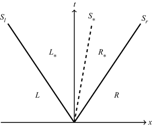
The Euler equations for molecular gas, (3.2), (3.3) and (3.4), which describe the leading-order terms of the expansion (3.1), have well-known solutions (Toro Reference Toro2013) for the Riemann problem with initial conditions similar to (2.7). Here, we consider the cases where the initial conditions result in an SCS solution structure as shown in figure 2. This solution structure consists of four constant regions –  $L$,
$L$,  $L_\ast$,
  $R_\ast$ and
  $R$ – separated by these three elementary waves where the variables
  ${\rho }_0$,
  $u_0$ and
  ${\theta }_0$ are discontinuous. The variables of the left (
 $L$) and right (
 $R$) regions have, throughout the time domain, the same values as their initial states. A left shock,
  $S_l$, separates the regions
  $L$ and
  $L_\ast$. Similarly, a right shock,
  $S_r$, separates the regions
  $R$ and
  $R_\ast$. The contact discontinuity,
  $S_\ast$, separates the regions
  $L_\ast$ and
  $R_\ast$, both referred to as the star region. The pressure is defined using the equation of state for dilute granular gas as (Reddy & Alam Reference Reddy and Alam2015; Sirmas & Radulescu Reference Sirmas and Radulescu2019)
 \begin{equation} p_0={\rho }_0{\theta }_0. \end{equation}
Figure 2. SCS solution structure.
The exact solution of the Riemann problem for SCS wave structure (Toro Reference Toro2013) is obtained by solving, using Newton's method, the following nonlinear equation for the pressure of the star region,  $p_{0,\ast }$,
 \begin{gather} (p_{0,\ast}-p_{0,L} ){\left[\frac{A_L}{p_{0,\ast}+B_L}\right]}^{{1}/{2}} + (p_{0,\ast}-p_{0,R} ){\left[\frac{A_R}{p_{0,\ast}+B_R}\right]}^{{1}/{2}} + (u_{0,R}-u_{0,L} )=0, \end{gather}
 \begin{gather} A_L=\frac{2}{(\gamma+1){\rho}_{0,L}}, \quad B_L=\frac{(\gamma-1)}{(\gamma+1)}p_{0,L}, \quad A_R=\frac{2}{(\gamma+1){\rho}_{0,R}}, \quad B_R=\frac{(\gamma-1)}{(\gamma+1)}p_{0,R}, \end{gather}
where  $\gamma ={5}/{3}$ is the specific heat ratio of dilute granular gas (Matveev Reference Matveev1983; Reddy & Alam Reference Reddy and Alam2015), the same value as that of monatomic molecular gas. After obtaining
  $p_{0,\ast }$, the velocity in the star region,
  $u_{0,\ast }$, which is equal to the speed of the contact discontinuity,
  $S_\ast$, is obtained using the following equation:
 \begin{align} u_{0,\ast}&=\frac{1}{2} (u_{0,R}+u_{0,L} ) +\frac{1}{2}\left\{ (p_{0,\ast}-p_{0,R} ) {\left[\frac{A_R}{p_{0,\ast}+B_R}\right]}^{{1}/{2}}\right. \nonumber\\ &\quad\left. -\,(p_{0,\ast}-p_{0,L} ) {\left[\frac{A_L}{p_{0,\ast}+B_L}\right]}^{{1}/{2}}\right\}. \end{align}
 The rest of the variables are obtained directly from the pressure in the star region,  $p_{0,\ast }$. The density in the region
  $L_\ast$ is
 \begin{equation} {\rho }_{0,L_\ast}={\rho }_{0,L}\left[\frac{p_{0,\ast}}{p_{0,L}} +\frac{\gamma -1}{\gamma +1}\right]{\left[{\left(\frac{\gamma -1}{\gamma +1}\right)\frac{p_{0,\ast}}{p_{0,L}}+1}\right]}^{{-}1}. \end{equation}
The speed of the left shock is
 \begin{equation} S_l=u_{0,L}-a_{0,L}{\left[\left(\frac{\gamma +1}{2\gamma}\right) \frac{p_{0,\ast}}{p_{0,L}}+\frac{\gamma -1}{2\gamma }\right]}^{{1}/{2}}, \end{equation}
where  $a$ is the speed of sound, which is defined for dilute granular gas as (Reddy & Alam Reference Reddy and Alam2015)
 \begin{equation} a=\sqrt{\gamma \theta }. \end{equation}
The density in the region  $R_\ast$ is
 \begin{equation} {\rho }_{0,R_\ast}={\rho }_{0,R} \left[\frac{p_{0,\ast}}{p_{0,R}}+\frac{\gamma -1}{\gamma +1}\right] {\left[{\left(\frac{\gamma -1}{\gamma +1}\right) \frac{p_{0,\ast}}{p_{0,R}}+1}\right]}^{{-}1}. \end{equation}
The speed of the right shock is
 \begin{equation} S_r=u_{0,R}+a_{0,R}{\left[\left(\frac{\gamma +1}{2\gamma}\right) \frac{p_{0,\ast}}{p_{0,R}}+\frac{\gamma -1}{2\gamma }\right]}^{{1}/{2}}. \end{equation}
 Note that the velocity and pressure are continuous across the contact whereas the density and temperature are discontinuous. In addition to the Euler equations for molecular gas, RH jump conditions across the shocks are used to derive this SCS solution at the leading order,  $O({\epsilon }^0)$.
3.2. Analytical solution of $O({\epsilon }^1)$

The governing equations, (3.5), (3.6) and (3.7), describing the evolution of the first-order terms of the expansion (3.1), constitute a linear hyperbolic system with source term. In vector form it reads
 \begin{equation} {\boldsymbol{\mathsf{C}}} {\boldsymbol{U}}_{t}+\boldsymbol{\mathsf{D}}{\boldsymbol{U}}_x=\boldsymbol{E}, \end{equation}
where the subscripts  $t$ and
  $x$ denote time and space derivatives. The vector
  $\boldsymbol {U}$ defines the variables of the first-order terms as
 \begin{equation} \boldsymbol{U}={[{\rho }_1\quad u_1 \quad {\theta }_1 ]}^\textrm{T}. \end{equation}
The matrices  $\boldsymbol{\mathsf{C}}$ and
  $\boldsymbol{\mathsf{D}}$ are
 \begin{gather} \boldsymbol{\mathsf{C}}=\left[ \begin{array}{@{}ccc@{}} 1 & 0 & 0 \\ u_0 & {\rho }_0 & 0 \\ {u_0}^2+3{\theta }_0 & 2{\rho }_0u_0 & 3{\rho }_0 \end{array} \right], \end{gather}
 \begin{gather}\boldsymbol{\mathsf{D}}=\left[ \begin{array}{@{}ccc@{}} u_0 & {\rho }_0 & 0 \\ {u_0}^2+{\theta }_0 & 2{\rho }_0u_0 & {\rho }_0 \\ {u_0}^3+5{\theta }_0u_0 & {\rho }_0 (3{u_0}^2+5{\theta }_0 ) & 5{\rho }_0u_0 \end{array} \right]. \end{gather}
The source term of (3.17) is given by the vector  $\boldsymbol {E}$ as
 \begin{equation} \boldsymbol{E}={ [ 0\quad 0\quad -{{\rho }_0}^2{{\theta }_0}^{3/2} ]}^\textrm{T}. \end{equation}
 The first step to solve this system is to multiply (3.17) by the inverse of the matrix  $\boldsymbol{\mathsf{C}}$,
 \begin{equation} {\boldsymbol{\mathsf{C}}}^{{-}1}=\left[ \begin{array}{@{}ccc@{}} 1 & 0 & 0 \\ {{-u}_0}{{\rho }_0}^{{-}1} & {{\rho }_0}^{{-}1} & 0 \\ { ({u_0}^2-3{\theta }_0 )}{ ({3{\rho }_0} )}^{{-}1} & {-2u_0}{ ({3{\rho }_0} )}^{{-}1} & { ({3{\rho }_0} )}^{{-}1} \end{array} \right], \end{equation}
which results in the following canonical form:
 \begin{align} \boldsymbol{U}_t+\boldsymbol{\mathsf{Y}}\boldsymbol{U}_x=\boldsymbol{\varGamma},\quad \boldsymbol{\varGamma} = {\tfrac{1}{3}}{ [ 0\quad 0 \quad {-{{\rho }_0}{{\theta }_0}^{3/2}} ]}^\textrm{T}, \quad \boldsymbol{\mathsf{Y}}=\left[ \begin{array}{@{}ccc@{}} u_0 & {\rho }_0 & 0 \\ {{\theta }_0}{{{\rho }_0}^{{-}1}} & u_0 & 1 \\ 0 & \tfrac{2}{3}{\theta }_0 & u_0 \end{array} \right]. \end{align}
The eigenvalues of the matrix  $\boldsymbol{\mathsf{Y}}$ are
 \begin{equation} {\lambda }^{(1)}=u_0-\sqrt{\gamma {\theta }_0},\quad {\lambda }^{(2)}=u_0,\quad {\lambda }^{(3)}=u_0+\sqrt{\gamma {\theta }_0}, \end{equation}
which are the same eigenvalues as for the leading-order problem describing the Euler equations for molecular gas; see (3.2), (3.3) and (3.4). Because the matrix  $\boldsymbol{\mathsf{Y}}$ is diagonalisable, it can be written as
 \begin{equation} \boldsymbol{\mathsf{Y}}=\boldsymbol{\mathsf{PGP}}^{{-}1}, \end{equation}
where  $\boldsymbol{\mathsf{G}}=\mathrm {diag}({\lambda }^{(1)},{\lambda }^{(2)},{\lambda }^{(3)})$ is the eigenvalues matrix and
  $\boldsymbol{\mathsf{P}}$ is the matrix of the right eigenvectors,
 \begin{equation} \boldsymbol{\mathsf{P}}=\left[ \begin{array}{@{}ccc@{}} {{-\rho }_0}{a_0}^{{-}1} & 1 & {{\rho }_0}{a_0}^{{-}1} \\ 1 & 0 & 1 \\ {-2{\theta }_0}{ (3a_0 )}^{{-}1} & -{{\theta }_0}{{\rho }_0}^{{-}1} & {2{\theta }_0}{ (3a_0 )}^{{-}1}\end{array} \right]. \end{equation}
 Thus, the first-order system,  $O({\epsilon }^1)$, can now be written as
 \begin{equation} \boldsymbol{U}_t+\boldsymbol{\mathsf{P}}\boldsymbol{\mathsf{G}}{\boldsymbol{\mathsf{P}}}^{{-}1}{\boldsymbol{U}}_x =\boldsymbol{\varGamma }. \end{equation}
Let
 \begin{equation} \boldsymbol{U}=\boldsymbol{\mathsf{P}}\boldsymbol{V}, \end{equation}
where  $\boldsymbol {V}={[v^{(1)}\ v^{(2)}\ v^{(3)}]}^\textrm {T}$ is the vector of Riemann variables. Since
  $\boldsymbol{\mathsf{P}}$ is constant (in each region), (3.27) can be written as
 \begin{equation} \boldsymbol{\mathsf{P}}{\boldsymbol{V}}_t+{\boldsymbol{\mathsf{P}}}\boldsymbol{\mathsf{G}}{\boldsymbol{V}_x} =\boldsymbol{\varGamma }. \end{equation}
Multiply (3.29) by the inverse of  $\boldsymbol{\mathsf{P}}$,
 \begin{equation} {\boldsymbol{\mathsf{P}}}^{{-}1}=\left[ \begin{array}{@{}ccc@{}} {-{\theta }_0}{ (2{\rho }_0a_0 )}^{{-}1} & \tfrac{1}{2} & -{ (2a_0 )}^{{-}1} \\ \tfrac{2}{5} & 0 & -{{\rho }_0}{ (\gamma {\theta }_0 )}^{{-}1} \\ {{\theta }_0}{ (2{\rho }_0a_0 )}^{{-}1} & \tfrac{1}{2} & { (2a_0 )}^{{-}1} \end{array} \right], \end{equation}
in order to decouple the system as
 \begin{equation} \boldsymbol{V}_t+\boldsymbol{\mathsf{G}}\boldsymbol{V}_x =\boldsymbol{F}, \end{equation}
where the source term,  $\boldsymbol {F}=\boldsymbol{\mathsf{P}}^{-1}\boldsymbol {\varGamma }$, is
 \begin{equation} \boldsymbol{F}=\frac{1}{6\gamma}{[{{\rho }_0{\theta }_0}{\sqrt{\gamma}} \quad 2{{{\rho }_0}^2\sqrt{{\theta }_0}} \quad -{{\rho }_0{\theta }_0}{\sqrt{\gamma}} ]}^\textrm{T}. \end{equation}
 Now, since the system of equations has been decoupled, the general solution for each Riemann variable,  $v^{(1)}$,
  $v^{(2)}$ and
  $v^{(3)}$, can be obtained independently. The governing equation for an arbitrary Riemann variable,
  $v^{(i)}$, where the superscript index
  $i=1,2,3$ denotes the order of the Riemann variable (first, second and third), can be written as
 \begin{equation} \frac{\partial v^{(i)}}{\partial t}+{\lambda }^{(i)}\frac{\partial v^{(i)}}{\partial x}=f^{(i)}, \end{equation}
where the characteristics,  ${\lambda }^{(i)}$, are given by (3.24) and the source terms,
  $f^{(i)}$, by (3.31). Transform (3.33) by changing the independent variables as
 \begin{equation} \varepsilon =t,\quad {\zeta }^{(i)}=x-{\lambda }^{(i)}t. \end{equation}
Note that the variable  $\varepsilon$ is global for all
  $v^{(i)}$, but the variable
  ${\zeta }^{(i)}$ is not global because it depends on the characteristics,
  ${\lambda }^{(i)}$, which are different for each Riemann variable,
  $v^{(i)}$.
The derivatives of the new variables  $(\varepsilon ,{\zeta }^{(i)} )$ with respect to the old variables
  $(t,x )$ are
 \begin{equation} \frac{\partial \varepsilon }{\partial t}=1,\quad \frac{\partial \varepsilon }{\partial x}=0,\quad \frac{\partial {\zeta }^{(i)}}{\partial t}={-}{\lambda }^{(i)},\quad \frac{\partial {\zeta }^{(i)}}{\partial x}=1. \end{equation}
Using the chain rule and (3.35) to transform the time and space derivatives of  $v^{(i)}$ from the old coordinate system
  $(t,x )$ to the new one
  $(\varepsilon ,{\zeta }^{(i)} )$ as
 \begin{equation} \frac{\partial v^{(i)}}{\partial t}=\frac{\partial v^{(i)}}{\partial \varepsilon }-{\lambda }^{(i)}\frac{\partial v^{(i)}}{\partial {\zeta }^{(i)}},\quad \frac{\partial v^{(i)}}{\partial x}=\frac{\partial v^{(i)}}{\partial {\zeta }^{(i)}}. \end{equation}
 By substituting (3.36) into (3.33), we obtain the governing equation for an arbitrary Riemann variable,  $v^{(i)}$, as a function of the independent variable,
  $\varepsilon$, as
 \begin{equation} \frac{\partial v^{(i)}}{\partial \varepsilon }=f^{(i)}, \end{equation}
whose general solution is obtained by integrating with respect to  $\varepsilon$ as
 \begin{equation} v^{(i)} (\varepsilon ,{\zeta }^{(i)} )=f^{(i)}\varepsilon +g^{(i)} ({\zeta}^{(i)} ), \end{equation}
where  $g^{(i)}({\zeta }^{(i)})$ is an integration function to be determined from the initial conditions. It is obvious that the initial conditions along the line
  $t=0$ are zero for all Riemann variables,
  $v^{(1)}$,
  $v^{(2)}$ and
  $v^{(3)}$, as expected for problems solved by regular perturbation of the governing equations. However, these initial conditions along the line
  $t=0$ do not give enough information to solve the Cauchy problem for the first-order hyperbolic system of equations,
  $O({\epsilon }^1)$. In (3.33), the slopes of the linear characteristic lines,
  ${\lambda }^{(i)}$, and the source terms,
  $f^{(i)}$, jump from one region to another because, in principle, the solution of the leading-order system,
  $O({\epsilon }^0)$, is discontinuous along the lines
  $S_l$,
  $S_\ast$ and
  $S_r$ as shown in figure 2. The jump in the characteristic lines,
  ${\lambda }^{(i)}$, means that the independent variable,
  ${\zeta }^{(i)}$, also jumps from one region to another, see (3.34), resulting in the same discontinuous domain of the leading-order system shown in figure 2. Accordingly, we need to specify a procedure to prescribe the initial conditions for the star regions,
  $L_\ast$ and
  $R_\ast$. An assumption is made now with regards to the jump in
  $v^{(1)}$,
  $v^{(2)}$ and
  $v^{(3)}$ at the discontinuities. We will not apply RH jump conditions for
  $O({\epsilon }^1)$, but we will assume, unless the characteristic structure shows otherwise, that each Riemann variable is continuous across the domain regions. With regards to the solution sequence in the regions
  $L$,
$L$,  $L_\ast$,
  $R_\ast$ and
  $R$ for each
  $v^{(i)}$, we will apply a procedure based on its characteristic structure,
  ${\lambda }^{(i)}$, which is described in detail in the following sections.
3.2.1. First Riemann variable
Figure 3 shows the first characteristic field,  ${\lambda }^{(1)}$, associated with the first Riemann variable,
  $v^{(1)}$. This characteristic field impinges on the left shock,
  $S_l$, and crosses both the contact discontinuity,
  $S_\ast$, and the right shock,
  $S_r$, from the right (LeVeque Reference LeVeque2002, p. 262). This characteristic structure implies that the initial conditions of the left and right states have two independent ranges of influence. The range of influence of the initial left state (
 $t=0, x<0$) terminates at the left of
  $S_l$. On the other hand, the range of influence of the initial right state (
 $t=0, x>0$) terminates at the right of
  $S_l$. Based on this characteristic structure, we solve
  $v^{(1)}$ in two independent cycles, each of which describes one of these ranges of influence.

Figure 3. Structure of the first characteristic field,  ${\lambda }^{(1)}$.
In the first cycle, we start from the initial left state and solve up to  $S_l$ approaching it from the left. In the second cycle, we start from the initial right state and solve up to
  $S_l$ approaching it from the right. As shown in figure 3, the first cycle consists of the region
  $L$ only. The solution of the Cauchy problem in this region is straightforward by prescribing the initial conditions at the line
  $t=0$,
  $x<0$, where
  $v^{(1)}=0$. The second solution cycle consists of three regions,
  $R$,
$R$,  $R_\ast$ and
  $L_\ast$, that should be solved sequentially. The solution in the region
  $R$ is obtained, in a similar way to the region
  $L$, by prescribing the initial conditions at the line
  $t=0$,
  $x>0$, where
  $v^{(1)}=0$. Subsequently, the solution in the region
  $R_\ast$ is obtained by prescribing a continuity initial condition for
  $v^{(1)}$ along
  $S_r$. Then, we solve the Cauchy problem for the region
  $L_\ast$, in a similar fashion, by prescribing a continuity initial condition for
  $v^{(1)}$ along
  $S_\ast$. Thus, the three regions of the second solution cycle are now connected to each other in a proper order that takes into account the domain of dependence and range of influence. The mathematical details of this solution procedure are as follows.
For the region  $L$, the initial condition is expressed as
 \begin{equation} {v_L}^{(1)} (\varepsilon =t=0,{{\zeta }_L}^{(1)} )=0. \end{equation}
Thus, the function of integration,  ${g_L}^{(1)}({{\zeta }_L}^{(1)})$, is zero, and the solution of
  $v^{(1)}$ in the region
  $L$ is
 \begin{equation} {v_L}^{(1)} (t,x )={f_L}^{(1)}t. \end{equation}
 Since the initial condition of the region  $R$ has similar form to that of
  $L$ (3.39), it is straightforward to show that the solution of
  $v^{(1)}$ in the region
  $R$ is
 \begin{equation} {v_R}^{(1)} (t,x )={f_R}^{(1)}t. \end{equation}
 Now, to determine the solution of  $v^{(1)}$ in the region
  $R_\ast$, we write the general solution as
 \begin{equation} {v_{R_\ast}}^{(1)} (\varepsilon ,{{\zeta }_{R_\ast}}^{(1)} ) ={f_{R_\ast}}^{(1)}\varepsilon+{g_{R_\ast}}^{(1)} ({{\zeta }_{R_\ast}}^{(1)} ). \end{equation}
The initial curve of the region  $R_\ast$ coincides with the right shock location whose equation is
 \begin{equation} t=\frac{x}{S_r}. \end{equation}
The initial condition for  $v^{(1)}$ in the region
  $R_\ast$ is defined along
  $S_r$ using the continuity assumption of
  $v^{(1)}$ as
 \begin{equation} {{v}_{R_\ast}}^{(1)}\left(t=\frac{x}{S_r},x\right) ={v_R}^{(1)}\left(t=\frac{x}{S_r},x\right). \end{equation}
This initial condition should be expressed in terms of the transformed variables  $(\varepsilon ,{{\zeta }_{R_\ast }}^{(1)})$ in order to obtain the function of integration,
  ${g_{R_\ast }}^{(1)}({{\zeta }_{R_\ast }}^{(1)})$. Since the transformation of the time variable from
  $(t,x)$ to
  $(\varepsilon ,{{\zeta }_{R_\ast }}^{(1)})$ is global for all regions,
  $t=\varepsilon$, equation (3.41) in the coordinates
  $(\varepsilon ,{{\zeta }_{R_\ast }}^{(1)})$ is
 \begin{equation} {v_R}^{(1)} (\varepsilon ,{{\zeta }_{R_\ast}}^{(1)} )={f_R}^{(1)}\varepsilon. \end{equation}
 Moreover, it is straightforward by using (3.34) to express the old variables  $(t,x)$ in terms of the new variables
  $(\varepsilon ,{{\zeta }_{R_\ast }}^{(1)})$ as
 \begin{equation} t=\varepsilon,\quad x={{\zeta }_{R_\ast}}^{(1)}+{{\lambda }_{R_\ast}}^{(1)}\varepsilon. \end{equation}
Substituting (3.46) into (3.43) gives the initial curve of the region  $R_\ast$ in terms of the transformed variables
  $(\varepsilon ,{{\zeta }_{R_\ast }}^{(1)})$ as
 \begin{equation} \varepsilon =\frac{{{\zeta }_{R_\ast}}^{(1)}}{S_r-{{\lambda }_{R_\ast}}^{(1)}}. \end{equation}
Now, substituting (3.47) into (3.42) and (3.45) gives the left- and right-hand sides of (3.44), respectively. This enables us to obtain the integration function,
 \begin{equation} {g_{R_\ast}}^{(1)} ({{\zeta}_{R_\ast}}^{(1)} ) =\left[\frac{{f_R}^{(1)}-{f_{R_\ast}}^{(1)}}{S_r-{{\lambda }_{R_\ast}}^{(1)}}\right]{{\zeta }_{R_\ast}}^{(1)}. \end{equation}
By substituting (3.48) into the general solution in the region  $R_\ast$, (3.42), we obtain the solution in terms of the new variables
  $(\varepsilon ,{{\zeta }_{R_\ast }}^{(1)})$ as
 \begin{equation} {v_{R_\ast}}^{(1)}={f_{R_\ast}}^{(1)}\varepsilon +\left[\frac{{f_R}^{(1)}-{f_{R_\ast}}^{(1)}}{S_r-{{\lambda }_{R_\ast}}^{(1)}}\right]{{\zeta }_{R_\ast}}^{(1)}. \end{equation}
The last step in obtaining  ${v_{R_\ast }}^{(1)}$ is to transform (3.49) from
  $(\varepsilon ,{{\zeta }_{R_\ast }}^{(1)})$ to
  $(t,x)$ by inverting (3.46), which has a similar form to (3.34), and substituting it into (3.49) as
 \begin{equation} \left.\begin{gathered} {v_{R_\ast}}^{(1)}={c_{R_\ast}}^{(1)}t+{b_{R_\ast}}^{(1)}x,\\ {c_{R_\ast}}^{(1)} =\frac{{f_{R_\ast}}^{(1)}S_r-{f_R}^{(1)}{{\lambda }_{R_\ast}}^{(1)}}{S_r-{{\lambda }_{R_\ast}}^{(1)}},\quad {b_{R_\ast}}^{(1)} = \frac{{f_R}^{(1)}-{f_{R_\ast}}^{(1)}}{S_r-{{\lambda }_{R_\ast}}^{(1)}}. \end{gathered}\right\}\end{equation}
 Now, we shall obtain the solution in the region  $L_\ast$ using a similar procedure to that for
  $R_\ast$. The general solution in the region
  $L_\ast$ is similar to (3.38) as
 \begin{equation} {v_{L_\ast}}^{(1)} (\varepsilon ,{{\zeta}_{L_\ast}}^{(1)} ) ={f_{L_\ast}}^{(1)}\varepsilon+{g_{L_\ast}}^{(1)} ({{\zeta }_{L_\ast}}^{(1)} ). \end{equation}
Using the continuity assumption, the initial condition of the region  $L_\ast$ is defined along the contact discontinuity,
  $S_\ast$, in a similar fashion to (3.44) as
 \begin{equation} {{v}_{L_\ast}}^{(1)}\left(t=\frac{x}{S_\ast},x\right) ={{v}_{R_\ast}}^{(1)}\left(t=\frac{x}{S_\ast},x\right). \end{equation}
For the region  $L_\ast$, the coordinate transformation from
  $(t,x)$ to
  $(\varepsilon ,{{\zeta }_{L_\ast }}^{(1)})$ is similar to (3.46), but the jump in the characteristic slope from
  ${{\lambda }_{R_\ast }}^{(1)}$ to
  ${{\lambda }_{L_\ast }}^{(1)}$ should be taken into account as
 \begin{equation} t=\varepsilon, \quad x={{\zeta }_{L_\ast}}^{(1)}+{{\lambda }_{L_\ast}}^{(1)}\varepsilon. \end{equation}
Substitute (3.53) into (3.50) in order to obtain  ${{v}_{R_\ast }}^{(1)}$ as a function of the new coordinates
  $(\varepsilon ,{{\zeta }_{L_\ast }}^{(1)})$ as
 \begin{equation} {v_{R_\ast}}^{(1)} (\varepsilon ,{{\zeta}_{L_\ast}}^{(1)} ) = [{c_{R_\ast}}^{(1)}+{b_{R_\ast}}^{(1)}{{\lambda }_{L_\ast}}^{(1)} ]\varepsilon +{b_{R_\ast}}^{(1)}{{\zeta }_{L_\ast}}^{(1)}. \end{equation}
 The initial curve of the region  $L_\ast$ is along the contact discontinuity,
  $S_\ast$, which is defined in the new coordinates
  $(\varepsilon ,{{\zeta }_{L_\ast }}^{(1)})$ in a similar fashion to (3.47) as
 \begin{equation} \varepsilon =\frac{{{\zeta }_{L_\ast}}^{(1)}}{S_\ast{-}{{\lambda }_{L_\ast}}^{(1)}}. \end{equation}
Substituting (3.55) into (3.54) gives  ${v_{R_\ast }}^{(1)}$ at
  $S_\ast$ in terms of
  ${{\zeta }_{L_\ast }}^{(1)}$ as
 \begin{equation} {v_{R_\ast}}^{(1)}\left(\varepsilon =\frac{{{\zeta }_{L_\ast}}^{(1)}}{S_\ast{-}{{\lambda }_{L_\ast}}^{(1)}}, {{\zeta}_{L_\ast}}^{(1)}\right) =\left[\frac{{c_{R_\ast}}^{(1)}+{b_{R_\ast}}^{(1)}S_\ast}{S_\ast{-}{{\lambda }_{L_\ast}}^{(1)}}\right]{{\zeta }_{L_\ast}}^{(1)}. \end{equation}
Substituting (3.55) into (3.51) gives  ${v_{L_\ast }}^{(1)}$ at
  $S_\ast$ in terms of
  ${{\zeta }_{L_\ast }}^{(1)}$ as
 \begin{equation} {v_{L_\ast}}^{(1)}\left(\varepsilon =\frac{{{\zeta }_{L_\ast}}^{(1)}}{S_\ast{-}{{\lambda }_{L_\ast}}^{(1)}},\ {{\zeta}_{L_\ast}}^{(1)}\right) ={f_{L_\ast}}^{(1)} \left[\frac{{{\zeta }_{L_\ast}}^{(1)}}{S_\ast{-}{{\lambda }_{L_\ast}}^{(1)}}\right]+{g_{L_\ast}}^{(1)} ({{\zeta }_{L_\ast}}^{(1)} ). \end{equation}
To obtain the integration function, substitute (3.56) and (3.57) into (3.52), resulting in
 \begin{equation} {g_{L_\ast}}^{(1)} ({{\zeta}_{L_\ast}}^{(1)} ) =\left[\frac{{c_{R_\ast}}^{(1)}+{b_{R_\ast}}^{(1)}S_\ast{-}{f_{L_\ast}}^{(1)}} {S_\ast{-}{{\lambda}_{L_\ast}}^{(1)}}\right]{{\zeta }_{L_\ast}}^{(1)}. \end{equation}
After obtaining  ${g_{L_\ast }}^{(1)}({{\zeta }_{L_\ast }}^{(1)})$, we need to transform the solution in the region
  $L_\ast$, given by (3.51) and (3.58), from
  $(\varepsilon ,{{\zeta }_{L_\ast }}^{(1)})$ to
  $(t,x)$ by inverting equation (3.53), which results in the final solution in the region
  $L_\ast$ as
 \begin{equation} \left.\begin{gathered} {v_{L_\ast}}^{(1)}(t,x) = [{f_{L_\ast}}^{(1)}-q^{(1)}{{\lambda}_{L_\ast}}^{(1)} ]t+q^{(1)}x, \\ q^{(1)} =\frac{{c_{R_\ast}}^{(1)}+{b_{R_\ast}}^{(1)}S_\ast{-}{f_{L_\ast}}^{(1)}} {S_\ast{-}{{\lambda}_{L_\ast}}^{(1)}}, \end{gathered}\right\} \end{equation}
where  ${c_{R_\ast }}^{(1)}$ and
  ${b_{R_\ast }}^{(1)}$ are given by the solution of the region
  $R_\ast$ as shown in (3.50).
Now, we have obtained  $v^{(1)}$ in the four regions of the domain,
  $L$,
$L$,  $R$,
$R$,  $R_\ast$ and
  $L_\ast$, as given by (3.40), (3.41), (3.50) and (3.59), respectively. The solution shows that both outer regions,
  $L$ and
  $R$, are linear functions of time, and the star regions,
  $L_\ast$ and
  $R_\ast$, are linear functions of both time and space. The solution of
  $v^{(1)}$ is continuous across all the regions except at the left shock,
  $S_l$, which separates the regions
  $L$ and
  $L_\ast$. In principle, the slope of
  $v^{(1)}$ jumps across all regions because it is a function of the solution of the leading-order system.
3.2.2. Second Riemann variable
Figure 4 shows the second characteristic field,  ${\lambda }^{(2)}$, associated with the second Riemann variable,
  $v^{(2)}$. This characteristic field is parallel to
  $S_\ast$ on both its sides and crosses
  $S_l$ from the left and
  $S_r$ from the right. Similar to
  $v^{(2)}$, this characteristic structure implies that there are two independent ranges of influence and accordingly two solution cycles that meet at
  $S_\ast$. In the first solution cycle, we start from the initial left state and solve for
  $L$ and
  $L_\ast$ until we reach
  $S_\ast$ from the left. In the second solution cycle, we start from the initial right state and solve for
  $R$ and
  $R_\ast$ until we reach
  $S_\ast$ from the right. The initial conditions for both
  $L$ and
  $R$ are zero at the line
  $t=0$, and those for
  $L_\ast$ and
  $R_\ast$ assume continuous
  $v^{(2)}$ along
  $S_l$ and
  $S_r$, respectively. The mathematical details are as follows.

Figure 4. Structure of the second characteristic field,  ${\lambda }^{(2)}$.
For the first solution cycle, we start with the region  $L$ whose solution has the same form as the first Riemann variable,
  ${v_L}^{(1)}$, given by (3.40), as
 \begin{equation} {v_L}^{(2)} (t,x )={f_L}^{(2)}t. \end{equation}
 In the region  $L_\ast$, the general solution is
 \begin{equation} {v_{L_\ast}}^{(2)}(\varepsilon ,{{\zeta }_{L_\ast}}^{(2)})={f_{L_\ast}}^{(2)}\varepsilon +{g_{L_\ast}}^{(2)}({{\zeta }_{L_\ast}}^{(2)}). \end{equation}
The initial condition of the region  $L_\ast$ is based on the continuous assumption of
  $v^{(2)}$ at the left shock,
 \begin{equation} {{v}_{L_\ast}}^{(2)}\left(t=\frac{x}{S_l},x\right) ={v_L}^{(2)}\left(t=\frac{x}{S_l},x\right). \end{equation}
Since the transformation of the time variable from  $(t,x)$ to
  $(\varepsilon ,{{\zeta }_{L_\ast }}^{(2)})$ is global for all regions,
  $t=\varepsilon$, equation (3.60) in the new coordinates
  $(\varepsilon ,{{\zeta }_{L_\ast }}^{(2)})$ is
 \begin{equation} {v_L}^{(2)} (\varepsilon ,{{\zeta }_{L_\ast}}^{(2)} )={f_L}^{(2)}\varepsilon . \end{equation}
Similar to (3.47) and (3.55), the initial curve of the region  $L_\ast$ is defined in
  $(\varepsilon ,{{\zeta }_{L_\ast }}^{(2)})$ as
 \begin{equation} \varepsilon =\frac{{{\zeta }_{L_\ast}}^{(2)}}{S_l-{{\lambda }_{L_\ast}}^{(2)}}. \end{equation}
Substituting (3.64) into (3.63) gives  ${v_L}^{(2)}$ at the left shock,
  $S_l$, in terms of
  ${{\zeta }_{L_\ast }}^{(2)}$ as
 \begin{equation} {v_L}^{(2)}\left(\varepsilon =\frac{{{\zeta }_{L_\ast}}^{(2)}}{S_l-{{\lambda }_{L_\ast}}^{(2)}},{{\zeta}_{L_\ast}}^{(2)}\right) =\left[\frac{{f_L}^{(2)}}{S_l-{{\lambda }_{L_\ast}}^{(2)}}\right]{{\zeta }_{L_\ast}}^{(2)}. \end{equation}
By substituting (3.64) into (3.61), we obtain  ${v_{L_\ast }}^{(2)}$ at
  $S_l$ in terms of
  ${{\zeta }_{L_\ast }}^{(2)}$ as
 \begin{equation} {v_{L_\ast}}^{(2)}\left(\varepsilon =\frac{{{\zeta }_{L_\ast}}^{(2)}}{S_l-{{\lambda }_{L_\ast}}^{(2)}},{{\zeta}_{L_\ast}}^{(2)}\right) =\left[\frac{{f_{L_\ast}}^{(2)}}{S_l-{{\lambda }_{L_\ast}}^{(2)}}\right]{{\zeta }_{L_\ast}}^{(2)}+{g_{L_\ast}}^{(2)} ({{\zeta }_{L_\ast}}^{(2)} ). \end{equation}
Substituting (3.65) and (3.66) into (3.62) enables us to obtain the function of integration,
 \begin{equation} {g_{L_\ast}}^{(2)} ({{\zeta}_{L_\ast}}^{(2)} ) =\left[\frac{{f_L}^{(2)}-{f_{L_\ast}}^{(2)}}{S_l-{{\lambda }_{L_\ast}}^{(2)}}\right]{{\zeta }_{L_\ast}}^{(2)}. \end{equation}
Thus, the final solution in the region  $L_\ast$ in the new coordinates
  $(\varepsilon ,{{\zeta }_{L_\ast }}^{(2)})$ is
 \begin{equation} {v_{L_\ast}}^{(2)} (\varepsilon ,{{\zeta}_{L_\ast}}^{(2)} ) ={f_{L_\ast}}^{(2)}\varepsilon +\left[\frac{{f_L}^{(2)}-{f_{L_\ast}}^{(2)}}{S_l-{{\lambda }_{L_\ast}}^{(2)}}\right]{{\zeta }_{L_\ast}}^{(2)}. \end{equation}
 Now, to transform equation (3.68) back to the coordinates  $(t,x)$, we adapt (3.34) to the region
  $L_\ast$ and the second Riemann variable,
  $v^{(2)}$, as
 \begin{equation} \varepsilon =t, \quad {{\zeta }_{L_\ast}}^{(2)}=x-{{\lambda}_{L_\ast}}^{(2)}t, \end{equation}
which when substituted into (3.68) gives the solution of  ${v_{L_\ast }}^{(2)}$ in
  $(t,x)$ as
 \begin{equation} \left.\begin{gathered} {v_{L_\ast}}^{(2)} (t,x )={c_{L_\ast}}^{(2)}t+{b_{L_\ast}}^{(2)}x, \\ {c_{L_\ast}}^{(2)}=\frac{{f_{L_\ast}}^{(2)}S_l-{f_L}^{(2)}{{\lambda }_{L_\ast}}^{(2)}}{S_l-{{\lambda }_{L_\ast}}^{(2)}}, \quad {b_{L_\ast}}^{(2)}= \frac{{f_L}^{(2)}-{f_{L_\ast}}^{(2)}}{S_l-{{\lambda }_{L_\ast}}^{(2)}}. \end{gathered}\right\}\end{equation}
 We have so far obtained the solution of  $v^{(2)}$ in the regions
  $L$ and
  $L_\ast$, reaching the contact discontinuity,
  $S_\ast$, from the left in the first solution cycle. To start the second cycle, the solution of
  ${v_R}^{(2)}$ has the same form as
  ${v_R}^{(1)}$, given by (3.41), as
 \begin{equation} {v_R}^{(2)}={f_R}^{(2)}t. \end{equation}
 In the region  $R_\ast$, the general solution is
 \begin{equation} {v_{R_\ast}}^{(2)}={f_{R_\ast}}^{(2)}\varepsilon +{g_{R_\ast}}^{(2)} ({{\zeta }_{R_\ast}}^{(2)} ). \end{equation}
In order to obtain the solution in the region  $R_\ast$, we follow a similar procedure to that used for the region
  $L_\ast$. We equate the value of the second Riemann variable in the region
  $R$ to that of the region
  $R_\ast$ along the right shock,
  $S_r$, resulting in the solution being
 \begin{equation} \left.\begin{gathered} {v_{R_\ast}}^{(2)}(t,x)={c_{R_\ast}}^{(2)}t+{b_{R_\ast}}^{(2)}x,\\ {c_{R_\ast}}^{(2)}=\frac{{f_{R_\ast}}^{(2)}S_r-{f_R}^{(2)}{{\lambda }_{R_\ast}}^{(2)}}{S_r-{{\lambda }_{R_\ast}}^{(2)}}, \quad {b_{R_\ast}}^{(2)}= \frac{{f_R}^{(2)}-{f_{R_\ast}}^{(2)}}{S_r-{{\lambda }_{R_\ast}}^{(2)}}, \end{gathered}\right\} \end{equation}
which ends the second cycle of the solution for  $v^{(2)}$ on the right of the contact discontinuity,
  $S_\ast$.
Now, we have obtained the solution of  $v^{(2)}$ in the four regions of the domain,
  $L$,
$L$,  $L_\ast$,
  $R_\ast$ and
  $R$, as given by (3.60), (3.70), (3.71) and (3.73), respectively. Note that, in (3.70) and (3.73), both
  ${{\lambda }_{R_\ast }}^{(2)}$ and
  ${{\lambda }_{L_\ast }}^{(2)}$ are equal to
  $S_\ast$ because
  ${\lambda }^{(2)}$ is linearly degenerate (LeVeque Reference LeVeque2002; Toro Reference Toro2013). In a similar behaviour to that of
  $v^{(1)}$, both outer regions,
  $L$ and
  $R$, are linear functions of time, and the star regions,
  $L_\ast$ and
  $R_\ast$, are linear functions of both time and space. The solution of
  $v^{(2)}$ is continuous across all the regions except at the contact discontinuity,
  $S_\ast$, which separates
  $L_\ast$ and
  $R_\ast$. Furthermore, the slope of
  $v^{(2)}$ has a similar behaviour to that of
  $v^{(1)}$: it jumps across all regions because it is a function of the solution of the leading-order system.
3.2.3. Third Riemann variable
Figure 5 shows the third characteristic field,  ${\lambda }^{(3)}$, associated with the third Riemann variable,
  $v^{(3)}$. The procedure used to obtain
  $v^{(3)}$ in the four domain regions,
  $L$,
$L$,  $L_\ast$,
  $R_\ast$ and
  $R$, is similar to that for
  $v^{(1)}$. However, the two cycles of solution are different because, for the case of
  $v^{(3)}$, its characteristics field,
  ${\lambda }^{(3)}$, impinges on the right shock,
  $S_r$, and crosses both
  $S_l$ and
  $S_\ast$ from the left. Thus, we start the first solution cycle from the line
  $t=0$,
  $x<0$, and solve in the regions
  $L$,
$L$,  $L_\ast$ and
  $R_\ast$ sequentially. Again, the initial condition of the region
  $L$ is zero. The regions
  $L_\ast$ and
  $R_\ast$ are connected to the regions
  $L$ and
  $L_\ast$, respectively, using the continuity assumption of
  $v^{(3)}$ along the corresponding discontinuities. In the second solution cycle, the initial condition is defined along the line
  $t=0$,
  $x>0$, to solve in the region
  $R$ approaching
  $S_r$ from the right. The mathematical details are described briefly as follows.

Figure 5. Structure of the third characteristic field,  ${\lambda }^{(3)}$.
For the first solution cycle of  $v^{(3)}$, we start with the region
  $L$, whose solution has the same form as the first and second Riemann variables, given by (3.40) and (3.60), as
 \begin{equation} {v_L}^{(3)}(t,x)={f_L}^{(3)}t. \end{equation}
 For the region  $L_\ast$, the general solution in the new coordinates
  $(\varepsilon ,{{\zeta }_{L_\ast }}^{(3)})$ is
 \begin{equation} {v_{L_\ast}}^{(3)} (\varepsilon ,{{\zeta}_{L_\ast}}^{(3)} ) ={f_{L_\ast}}^{(3)}\varepsilon+{g_{L_\ast}}^{(3)} ({{\zeta}_{L_\ast}}^{(3)} ), \end{equation}
and its initial curve is the line along the left shock,  $S_l$, which is defined in
  $(\varepsilon ,{{\zeta }_{L_\ast }}^{(3)})$ in a similar fashion to (3.64) as
 \begin{equation} \varepsilon =\frac{{{\zeta }_{L_\ast}}^{(3)}}{S_l-{{\lambda }_{L_\ast}}^{(3)}}. \end{equation}
Substituting (3.76) into (3.74) and noting that  $t=\varepsilon$, we get
  ${v_L}^{(3)}$ at
  $S_l$ as
 \begin{equation} {v_L}^{(3)}\left(\varepsilon = \frac{{{\zeta }_{L_\ast}}^{(3)}}{S_l-{{\lambda }_{L_\ast}}^{(3)}},\ {{\zeta}_{L_\ast}}^{(3)}\right) =\left[\frac{{f_L}^{(3)}}{S_l-{{\lambda }_{L_\ast}}^{(3)}}\right]{{\zeta }_{L_\ast}}^{(3)}, \end{equation}
and according to our assumption of continuous  $v^{(3)}$ along
  $S_l$, the initial condition for the region
  $L_\ast$ is defined as
 \begin{equation} {v_{L_\ast}}^{(3)}\left(\varepsilon =\frac{{{\zeta }_{L_\ast}}^{(3)}}{S_l-{{\lambda }_{L_\ast}}^{(3)}},{{\zeta }_{L_\ast}}^{(3)}\right)={v_L}^{(3)}\left(\varepsilon =\frac{{{\zeta }_{L_\ast}}^{(3)}}{S_l-{{\lambda }_{L_\ast}}^{(3)}}, {{\zeta }_{L_\ast}}^{(3)}\right). \end{equation}
Substituting (3.75) into the left-hand side of (3.78) and (3.77) into its right-hand side enables us to obtain the integration function,
 \begin{equation} {g_{L_\ast}}^{(3)} ({{\zeta}_{L_\ast}}^{(3)} ) =\left[\frac{{f_L}^{(3)}-{f_{L_\ast}}^{(3)}}{S_l-{{\lambda }_{L_\ast}}^{(3)}}\right]{{\zeta }_{L_\ast}}^{(3)}. \end{equation}
Substituting (3.79) into the general solution of  ${v_{L_\ast }}^{(3)}$, given by (3.75), then transforming to
  $(t,x)$, according to (3.34), results in the solution of
  ${v}^{(3)}$ in the region
  $L_\ast$,
 \begin{equation} \left.\begin{gathered} {v_{L_\ast}}^{(3)}(t,x)={c_{L_\ast}}^{(3)}t +{b_{L_\ast}}^{(3)}x, \\ {c_{L_\ast}}^{(3)} =\frac{{f_{L_\ast}}^{(3)}S_l-{f_L}^{(3)}{{\lambda }_{L_\ast}}^{(3)}}{S_l-{{\lambda}_{L_\ast}}^{ (3)}}, \quad {b_{L_\ast}}^{(3)} =\frac{{f_L}^{(3)}-{f_{L_\ast}}^{(3)}}{S_l-{{\lambda }_{L_\ast}}^{(3)}}. \end{gathered}\right\} \end{equation}
 The subsequent step is to solve in the region  $R_\ast$ whose general solution is
 \begin{equation} {v_{R_\ast}}^{(3)} (\varepsilon ,{{\zeta}_{R_\ast}}^{(3)} ) ={f_{R_\ast}}^{(3)}\varepsilon+{g_{R_\ast}}^{(3)} ({{\zeta }_{R_\ast}}^{(3)} ). \end{equation}
The initial curve of the region  $R_\ast$ coincides with the contact discontinuity,
  $S_\ast$, which is defined in the new coordinates
  $(\varepsilon ,{{\zeta }_{R_\ast }}^{(3)})$ in a similar fashion to (3.55) as
 \begin{equation} \varepsilon =\frac{{{\zeta }_{R_\ast}}^{(3)}}{S_\ast{-}{{\lambda }_{R_\ast}}^{(3)}}. \end{equation}
According to our assumption of continuous  $v^{(3)}$ along
  $S_\ast$, the initial condition of the region
  $R_\ast$ is
 \begin{equation} {v_{R_\ast}}^{(3)}\left(\varepsilon =\frac{{{\zeta }_{R_\ast}}^{(3)}}{S_\ast{-}{{\lambda }_{R_\ast}}^{(3)}},{{\zeta }_{R_\ast}}^{(3)}\right) ={v_{L_\ast}}^{(3)}\left(\varepsilon =\frac{{{\zeta }_{R_\ast}}^{(3)}}{S_\ast{-}{{\lambda }_{R_\ast}}^{(3)}},{{\zeta }_{R_\ast}}^{(3)}\right). \end{equation}
In order to obtain the right-hand side of (3.83), we need to write (3.80) in the new local coordinates of the region  $R_\ast$,
  $(\varepsilon ,{{\zeta }_{R_\ast }}^{(3)})$, by adapting the inverse of transformation (3.34) as
 \begin{equation} {v_{L_\ast}}^{(3)} (\varepsilon ,{{\zeta}_{R_\ast}}^{(3)} ) ={c_{L_\ast}}^{(3)}\varepsilon +{b_{L_\ast}} ^{(3)}[{{\zeta }_{R_\ast}}^{(3)}+{{\lambda }_{R_\ast}}^{(3)}\varepsilon ]. \end{equation}
In (3.81), the left-hand side is obtained by substituting (3.82) into (3.81), and the right-hand side is obtained by substituting (3.82) into (3.84). This results in obtaining the function of integration for the region  $R_\ast$ as
 \begin{equation} {g_{R_\ast}}^{(3)} ({{\zeta}_{R_\ast}}^{(3)} ) =\left[\frac{{c_{L_\ast}}^{(3)}+{b_{L_\ast}}^{(3)}S_\ast{-}{f_{R_\ast}}^{(3)}} {S_\ast{-}{{\lambda}_{R_\ast}}^{(3)}}\right]{{\zeta }_{R_\ast}}^{(3)}. \end{equation}
 To obtain the final solution of the third Riemann variable in the region  $R_\ast$,
  ${v_{R_\ast }}^{(3)}$, in terms of the original variables
  $(t,x)$, we apply the generic transformation (3.34) to both the general solution (3.81) and the integration function (3.85), resulting in
 \begin{equation} \left.\begin{gathered} {v_{R_\ast}}^{(3)}(t,x) = [{f_{R_\ast}}^{(3)}-q^{(3)}{{\lambda}_{R_\ast}}^{(3)} ]t+q^{(3)}x,\\ q^{(3)}=\frac{{c_{L_\ast}}^{(3)}+{b_{L_\ast}}^{(3)}S_\ast{-}{f_{R_\ast}}^{(3)}} {S_\ast{-}{{\lambda}_{R_\ast}}^{(3)}}, \end{gathered}\right\} \end{equation}
which ends the first solution cycle of the third Riemann variable  $v^{(3)}$ by reaching the left shock,
  $S_l$, from the left. The second cycle consists of solving
  $v^{(3)}$ in the region
  $R$ only, which is similar to both
  ${v_R}^{(1)}$ and
  ${v_R}^{(2)}$, as
 \begin{equation} {v_R}^{(3)}(t,x)={f_R}^{(3)}t. \end{equation}
 Now, we have obtained  $v^{(3)}$ in the four regions of the domain,
  $L$,
$L$,  $L_\ast$,
  $R_\ast$ and
  $R$, as given by (3.74), (3.80), (3.86) and (3.87), respectively. In a similar behaviour to that of
  $v^{(1)}$ and
  $v^{(2)}$, the solution shows that both outer regions,
  $L$ and
  $R$, are linear functions of time, and the star regions,
  $L_\ast$ and
  $R_\ast$, are linear functions of both time and space. The solution of
  $v^{(3)}$ is continuous across all regions except at the right shock,
  $S_r$, which separates the regions
  $R_\ast$ and
  $R$. Furthermore, the slope of
  $v^{(3)}$ has a similar behaviour to that of
  $v^{(1)}$ and
  $v^{(2)}$: it jumps across all regions, because it is a function of the solution of the leading-order system.
3.2.4. Primitive variables
After obtaining the Riemann variables vector,  $\boldsymbol {V}={[v^{(1)} \ v^{(2)}\ v^{(3)}]}^\textrm {T}$, in all four regions (
 $L$,
$L$,  $L_\ast$,
  $R_\ast$ and
  $R$), we transform it back to the primitive variables vector,
  $\boldsymbol {U}={[ {\rho }_1\ u_1\ {\theta }_1 ]}^\textrm {T}$, using (3.26) and (3.28) as
 \begin{gather} {\rho }_1={-}\left[\frac{{\rho}_0}{a_0}\right]v^{(1)}+v^{(2)} +\left[\frac{{\rho}_0}{a_0}\right]v^{(3)}, \end{gather}
 \begin{gather}u_1=v^{(1)}+v^{(3)}, \end{gather}
 \begin{gather}{\theta }_1={-}\left[\frac{2{\theta }_0}{3a_0}\right]v^{(1)} -\left[\frac{{\theta}_0}{{\rho }_0}\right]v^{(2)} +\left[\frac{2{\theta}_0}{3a_0}\right]v^{(3)}. \end{gather}
 Note that the coefficients of the Riemann variables in (3.88), (3.89) and (3.90) jump across the domain regions,  $L$,
$L$,  $L_\ast$,
  $R_\ast$ and
  $R$, because they are obtained from the solution of the leading-order problem,
  $O({\epsilon }^0)$; see § 3.1.
3.3. Solution structure and accuracy
Now, we have solved, analytically, the Riemann problem for dilute granular gas for the case of SCS wave structure using a regular perturbation method. Similar to molecular gas, the solution consists of four regions,  $L$,
$L$,  $L_\ast$,
  $R_\ast$ and
  $R$, separated by three discontinuities,
  $S_l$,
  $S_\ast$ and
  $S_r$. A key difference between this solution and that of molecular gas is that the variables in these regions are not, in principle, constant with time and space. The accuracy of our solution is first order in the domain regions, but the speeds of the shocks and contact discontinuity are of leading-order accuracy because the characteristics of the first-order problem are the same as those of the leading-order problem: straight lines in the
  $(x,t)$ plane. However, the strength of these discontinuities is not entirely of leading-order accuracy because the solution of the first-order problem permits discontinuities across these lines for all Riemann variables, which is carried to
  ${\rho }_1$,
  $u_1$ and
  ${\theta }_1$. We did not use RH conditions to obtain the jump in the Riemann variables across the discontinuous lines,
  $S_l$,
  $S_\ast$ and
  $S_r$, because this would require an iterative solution as the Riemann variables become coupled. Accordingly, the continuity assumption of the Riemann variables along some discontinuous lines was used in order to obtain an explicit analytical solution that is valid for early evolution time.
4. Numerical solution method
The analytical solution presented in § 3 is valid for small  $\epsilon$ and early evolution time. In order to test these assumptions, we solve, numerically, the Riemann problem for dilute granular gas given by (2.12), (2.13) and (2.14). This system of hyperbolic balance laws can be expressed in vector form as
 \begin{equation} \left.\begin{gathered} \boldsymbol{Q}_t+\boldsymbol{H}(\boldsymbol{Q})_x =\boldsymbol{Z}(\boldsymbol{Q}), \quad \boldsymbol{Q}={ [\rho \quad \rho u\quad \rho u^2+3\rho \theta ]}^\textrm{T},\\ \boldsymbol{H}(\boldsymbol{Q})={ [(\rho u)\quad (\rho u^2+\rho \theta ) \quad (\rho u^3+5\rho \theta u )]}^\textrm{T},\quad \boldsymbol{Z}(\boldsymbol{Q})={ [0 \quad 0 \quad -\epsilon {\rho }^2{\theta }^{3/2} ]}^\textrm{T}. \end{gathered}\right\}\end{equation}
Reddy & Alam (Reference Reddy and Alam2015) used a splitting technique to the solve this non-homogeneous system, which we use in this paper. For each computational time step, splitting techniques (Toro Reference Toro2013, pp. 531–542) consist of two successive steps. The first step is solving, using an appropriate shock-capturing technique, the conservative system
 \begin{equation} \boldsymbol{Q}^{ {h}}_t+\boldsymbol{H}(\boldsymbol{Q}^{ {h}})_x=0, \end{equation}
where the superscript  ${h}$ denotes the corresponding homogeneous variables. In the second step, the solution is updated for each time,
  $t_j$, using
  $\boldsymbol {Q}^{{h}}$ as the initial condition,
 \begin{equation} \boldsymbol{Q}_t=\boldsymbol{Z}(\boldsymbol{Q}),\quad \boldsymbol{Q} (x,t_j )=\boldsymbol{Q}^{ {h}} (x,t_j ). \end{equation}
 We implemented the relaxation scheme of Jin & Xin (Reference Jin and Xin1995), which was used by Reddy & Alam (Reference Reddy and Alam2015), to solve the conservative system (4.2). In our simulations, the relaxation parameter was  ${10}^{-8}$, the same value as used by Reddy & Alam (Reference Reddy and Alam2015), and the positive diagonal matrix was
  $\mathrm {diag}(1.0,1.68,5.045)$. We used a first-order upwind scheme with a uniform step size of
  ${1.5\times 10}^{-3}$ for spatial discretisation, and a second-order total variation diminishing Runge–Kutta splitting scheme with a uniform time step size of
  ${5\times 10}^{-5}$ for temporal discretisation, which resulted in a Courant–Friedrichs–Lewy number of
  $0.168$. For the solution of the second step (4.3a,b), we used the Euler method for time integration. Our code implementation and numerical parameters were verified by the excellent agreement of our results with Reddy & Alam (Reference Reddy and Alam2015); see § 5.3.
5. Results and discussion
The aim of this section is to understand the solution structure of the Riemann problem for dilute granular gas and to validate the assumptions of our approximate analytical solution. We compare our analytical solution (§ 3) with the numerical solution (§ 4) for three cases of initial conditions, i.e. symmetric, asymmetric and single shock, using different values of  $\epsilon$. The comparisons presented here are for the three primitive variables,
  $\rho$,
  $u$ and
  $\theta$, shown at early evolution times,
  $t=1$,
  $2$ and
  $4$.
$4$.
5.1. Symmetric
The symmetric case considered here is the collision between two opposite supersonic gas streams of equal Mach number,  ${Ma}_L={Ma}_R=1.2$. In molecular gas, the solution structure for this case consists of left and right shocks of equal strength travelling in opposite directions and a trivial, where both density and temperature do not jump, stationary contact discontinuity (Toro Reference Toro2013, p. 129).
Figures 6, 7 and 8 show comparisons between the analytical and numerical solutions for three values of the dissipation parameter:  $\epsilon =0.05$,
  $0.1$ and
  $0.2$, respectively. For all values of
  $\epsilon$, one can notice similar qualitative behaviour in the two solution approaches. At any time instant, the spatial profiles of all three variables, density, velocity and temperature, are uniform in the outer (
 $L$ and
  $R$) regions. Then each of these variables undergoes an equal jump – absolute value for velocity – across both the left and right shocks due to the symmetry of the initial conditions. One can also notice in all density and temperature profiles the stationary trivial contact discontinuity that separates the regions
  $L_\ast$ and
  $R_\ast$ at
  $x=0$. Across this contact discontinuity, the gradients of both density and temperature are discontinuous, but the velocity gradient is continuous. In the regions
  $L_\ast$ and
  $R_\ast$, all the variables change with both space and time. At any time instant, the density increases in the region
  $L_\ast$ (behind the left shock) and decreases in the region
  $R_\ast$ (increases behind the right shock) whereas the temperature has the opposite trend. Throughout the star region, the velocity is continuous and decreases monotonically.

Figure 6. Comparisons between analytical (solid) and numerical (dashed) solutions for symmetric initial conditions,  $\epsilon =0.05$.

Figure 7. Comparisons between analytical (solid) and numerical (dashed) solutions for symmetric initial conditions,  $\epsilon =0.1$.

Figure 8. Comparisons between analytical (solid) and numerical (dashed) solutions for symmetric initial conditions,  $\epsilon =0.2$.
By comparing the profiles at different time instants in the outer regions ( $L$ and
  $R$) for each value of
  $\epsilon$, it is noticed that both density and velocity are constant with time, but the granular temperature decreases due to inelastic collisions. In the star region, the maximum value of density and minimum value of granular temperature, both occurring at the contact discontinuity, increases and decreases with time, respectively. Note that the profiles of either half-spaces (
 $x>0$ or
  $x<0$) are qualitatively similar to a piston moving in quiescent granular gas in the moving-piston frame of reference (Matveev Reference Matveev1983; Goldshtein et al. Reference Goldshtein, Shapiro and Gutfinger1996a; Kamenetsky et al. Reference Kamenetsky, Goldshtein, Shapiro and Degani2000; Sirmas & Radulescu Reference Sirmas and Radulescu2019); see § 1.
After showing the consistent qualitative similarities between the two solution approaches, we now discuss the quantitative discrepancies. For a small value of dissipation parameter,  $\epsilon =0.05$, shown in figure 6, there is an excellent agreement between the two solution approaches, though there are slight discrepancies at later time,
  $t=4$. In figure 7, where the dissipation parameter is increased to a moderate value of
  $\epsilon =0.1$, discrepancies are noticed in the locations and strengths of both shocks as well as the density and temperature profiles, especially at
  $t=4$. The discrepancies in the locations of the shocks are expected because our analytical solution assumes straight-line characteristics, resulting in constant shock speeds that are equal to those of molecular gas. On the contrary, the characteristics of the full problem, solved numerically, are curved, resulting in variable shock speeds. The discrepancies in the strengths of the shocks are due to not using RH jump conditions in the analytical solution at
  $O({\epsilon }^1)$. The discrepancies in the star region profiles, for example the temperature, are due to these two effects as well as the neglected higher-order effects. In figure 8, where
  $\epsilon =0.2$, all these discrepancies become more pronounced even at earlier time,
  $t=2$.
5.2. Asymmetric
In this section, we consider the asymmetric case, where the left state is supersonic and the right state is at rest. This configuration is similar to that of Serna & Marquina (Reference Serna and Marquina2007) and Kamath & Du (Reference Kamath and Du2009). Here, the initial left Mach number is the same as that of § 5.1 at  ${Ma}_L=1.2$, but the initial right granular temperature is decreased to
  ${\theta }_R=0.6$. In contrast to § 5.1, the molecular gas solution for these initial conditions is not symmetric; thus, the contact discontinuity is not trivial.
Figures 9, 10 and 11 show comparisons between the analytical and numerical solutions for the same values of the dissipation parameter as used in § 5.1,  $\epsilon =0.05$,
  $0.1$ and
  $0.2$, respectively. Again, there is a consistent qualitative agreement between the two solution approaches. For all values of
  $\epsilon$ and
  $t$, the jump across the middle contact discontinuity is clear in the asymmetric profiles and gradients of both density and temperature. Similar to § 5.1, the density increases in the region
  $L_\ast$ (behind the left shock) and decreases in the region
  $R_\ast$ (increases behind the right shock) whereas the granular temperature has the opposite trend. Moreover, the velocity profiles and gradients are continuous along the contact (similar to molecular gas), and the velocity decreases in the star region (
 $L_\ast$ and
  $R_\ast$) between the two shocks. Similar to § 5.1, the maximum value of density and minimum value of granular temperature in the star region, both at the contact discontinuity, increases and decreases with time, respectively.

Figure 9. Comparisons between analytical (solid) and numerical (dashed) solutions for asymmetric initial conditions,  $\epsilon =0.05$.

Figure 10. Comparisons between analytical (solid) and numerical (dashed) solutions for asymmetric initial conditions,  $\epsilon =0.1$.

Figure 11. Comparisons between analytical (solid) and numerical (dashed) solutions for asymmetric initial conditions,  $\epsilon =0.2$.
In a similar behaviour to figure 6, there is excellent quantitative agreement between the analytical and numerical solutions using a small value of dissipation parameter of  $\epsilon =0.05$, as shown in figure 9. In figure 10, where the dissipation parameter is moderate at
  $\epsilon =0.1$, there are discrepancies between the two solution approaches, especially for later time,
  $t=4$. For a high dissipation parameter of
  $\epsilon =0.2$ shown in figure 11, the discrepancies between the two solution approaches are even more pronounced and keep increasing with time. Similar to figure 8, the noticed discrepancies are in the shock strengths and speeds as well as the density and temperature profiles in the star region. The speed of the contact discontinuity is, however, nearly identical in the two solution approaches.
5.3. Single shock
Here, our simulations employ the same initial conditions as in Reddy & Alam (Reference Reddy and Alam2015). The initial left state is supersonic at  ${Ma}_L=1.2$, and the initial right state is obtained using RH conditions for a stationary shock (Reddy & Alam Reference Reddy and Alam2015),
 \begin{gather} \frac{{\rho }_{0,R}}{{\rho }_{0,L}}=\frac{(\gamma +1){{Ma}_L}^2}{2+(\gamma -1){{Ma}_L}^2}=\frac{u_{0,L}}{u_{0,R}}, \end{gather}
 \begin{gather}\frac{{\theta }_R}{{\theta }_L}=\frac{(2\gamma {{Ma}_L}^2-(\gamma -1))((\gamma -1){{Ma}_L}^2+2)}{{(\gamma +1)}^2{{Ma}_L}^2}, \end{gather}
which shows that  ${\theta }_R=1.1948$,
  ${\rho }_R=1.2973$ and
  $u_R=1.1942$. Since
  $p_{0,R}>p_{0,L}$ and the following conditions are satisfied (Toro Reference Toro2013, pp. 119–126),
 \begin{equation} (u_{0,R}-u_{0,L} )+\frac{2a_R}{\gamma -1}\left[ {\left(\frac{p_{0,L}}{p_{0,R}}\right)}^{({\gamma -1})/{2\gamma }}-1\right]<0, \end{equation}
 \begin{equation}(u_{0,R}-u_{0,L} )+ (p_{0,R}-p_{0,L} ) {\left[\frac{A_L}{p_{0,R}+B_L}\right]}^{{1}/{2}}<0, \end{equation}
the wave structure for this case is SCS. The solution of the Riemann problem for molecular gas, see § 3.1, using these initial conditions is shown in table 1. Indeed, these initial conditions result in a stationary left shock wave for molecular gas. However, this left shock appears as if it is the only discontinuity because both the contact discontinuity,  $S_\ast$, and the right shock,
  $S_r$, are trivial with zero strength.
Table 1. Solution of the Riemann problem for molecular gas using the initial conditions of Reddy & Alam (Reference Reddy and Alam2015).
Figures 12, 13 and 14 show comparisons between the analytical and numerical solutions for dilute granular gas with  $\epsilon =0.1$,
  $0.2$ and
  $0.30299$, respectively. Note that, for the case of
  $\epsilon =0.30299$ shown in figure 14, the inelastic coefficient is 0.9, the same value as used by Reddy & Alam (Reference Reddy and Alam2015). Similar to §§ 5.1 and 5.2, it is clear that there is consistent qualitative agreement between the two solution approaches; moreover, there is very good quantitative agreement for
  $\epsilon =0.1$ at early evolution time; see figure 12.

Figure 12. Comparisons between analytical (solid) and numerical (dashed) solutions for single shock initial conditions,  $\epsilon =0.1$.

Figure 13. Comparisons between analytical (solid) and numerical (dashed) solutions for single shock initial conditions,  $\epsilon =0.2$.

Figure 14. Comparisons between analytical (solid) and numerical (dashed) solutions for single shock initial conditions,  $\epsilon =0.30299$.
In figures 12, 13 and 14, the density, velocity and temperature profiles show the propagation of a left shock, where these variables jump abruptly. The density behind the left shock (in the region  $L_\ast$) increases until reaching a maximum value at the trivial contact discontinuity. Then it decreases, in the region
  $R_\ast$, reaching a minimum value at the trivial right shock before remaining constant in the region
  $R$. This density profile was called ‘density overshoot’ by Reddy & Alam (Reference Reddy and Alam2015). In their Navier–Stokes simulations of this problem, this sharp variation in the density profiles was smeared due to the diffusive effects. Thus, Reddy & Alam (Reference Reddy and Alam2015) claimed that this ‘density overshoot’ is part of the shock layer, which is not true: these overshoots are mere signatures of the density increase in the region
  $L_\ast$ and its decrease in the region
  $R_\ast$,with its maximum value occurring at the contact discontinuity as consistently shown in §§ 5.1 and 5.2. The velocity and temperature profiles also show consistent behaviour where they vary in the star regions. Accordingly, in contrast to molecular gas, these initial conditions, given by (5.1) and (5.2), cannot be used to generate a single planar shock wave in granular gas. However, such a single shock wave can be generated, in either half-space, by the symmetric conditions shown in § 5.1, because the contact discontinuity is trivial and either the left or the right half-space contains a single shock wave.
6. Conclusions
In this paper, we studied the solutions of the Riemann problem for dilute granular gas using initial conditions that result in a shock–contact–shock (SCS) wave structure. We used a regular perturbation method to solve the problem analytically for a small value of the dissipation parameter that is valid for early evolution time. The leading order of the solution is that of molecular gas in which all the variables are constant in the domain regions –  $L$,
$L$,  $L_\ast$,
  $R_\ast$ and
  $R$ – but discontinuous across the three elementary waves. The first-order solution shows that all the variables in the star regions (
 $L_\ast$ and
  $R_\ast$) vary, in principle, with both space and time. In the outer regions (
 $L$ and
  $R$), the granular temperature is the only variable that varies with time due to inelastic collisions. The comparisons of our approximate analytical solution with the numerical solution of the full problem show excellent qualitative agreement in all the cases studied and good quantitative agreement for
  $\epsilon =0.05$ and
  ${0.1}$. Our solution shows that the ‘density overshoot’ reported by Reddy & Alam (Reference Reddy and Alam2015) is not part of the shock layer, but a mere signature of the density variation in the star regions between the left and right shocks, with its maximum value occurring at the contact discontinuity. Thus, an initial data structure that results in a single shock for molecular gas cannot generate a single shock structure for granular gas. Symmetric initial conditions can be used, however, to generate such structure.
Declaration of interest
The author reports no conflict of interest.


