


1 Introduction
A thin rectangular plate tumbles spontaneously along its longest axis as it falls in air (Maxwell Reference Maxwell1853). Tumbling generates lift, due to the so-called ‘Magnus effect’ (Magnus Reference Magnus1853), which causes the wing to drift horizontally (Mahadevan, Ryu & Samuel Reference Mahadevan, Ryu and Samuel1999). This tumbling-induced drift is one of many strategies exploited by seeds to fly away from parent trees and spread spatially (Vogel Reference Vogel1994). Other noteworthy strategies improving dispersal efficiency include: auto-rotation around a vertical axis (Norberg Reference Norberg1973; Lentink et al. Reference Lentink, Dickson, van Leeuwen and Dickinson2009; Varshney, Chang & Wang Reference Varshney, Chang and Wang2012; Lee, Lee & Sohn Reference Lee, Lee and Sohn2014); gliding (Azuma & Okuno Reference Azuma and Okuno1987); and vortex-induced drag enhancement (Greene & Johnson Reference Greene and Johnson1990; Cummins et al. Reference Cummins, Seale, Macente, Certini, Mastropaolo, Viola and Nakayama2018). While auto-rotation and drag enhancement lead to substantial increase in the seedpods’ flight time, they do not intrinsically generate drift and therefore rely on wind gusts to effectively carry the seed away from its parent tree. In contrast, the tumbling flight mode produce drift per se, and allows dispersion in windless or even breezy conditions (Matlack Reference Matlack1987), likely giving trees that rely on them, such as A. Altissima, an invasive species (Kowarik & Säumel Reference Kowarik and Säumel2007), a clear edge for efficient reproduction.

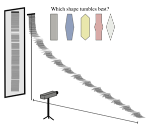
Figure 1. Experimental apparatus and methods. (a) Wings are tested by releasing them edge on with no linear or rotational velocity and measuring typical characteristics such as rotational speed  $\unicode[STIX]{x1D6FA}$ and descent angle
  $\unicode[STIX]{x1D6FD}$. (b) In vivo examples illustrating the variety of geometries of winged seedpods: Alsomitra macrocarpa (gliding); Acer griseum (auto-rotating); Ailanthus altissima (tumbling – this study). (c) The two families of planform shapes initially considered in this study. (d) Wings kinematics and performance were studied by means of a quasi-steady, quasi-two-dimensional model.
The dynamics of a tumbling plate is substantially more complicated than that of a fixed wing due to the complexity of the induced flow (Lugt Reference Lugt1983; Ruifeng Reference Ruifeng2015). This complication hinders analytical developments and has led to a large body of experiment-based studies, both in free fall and in a fixed, more controlled configuration (Dupleich Reference Dupleich1941; Smith Reference Smith1971; Iversen Reference Iversen1979; Lugt Reference Lugt1983; Andersen, Pesavento & Wang Reference Andersen, Pesavento and Wang2005b). The vast majority of these studies focused on the canonical case of a uniform rigid rectangular wing falling in air, or exposed to a constant stream of air. Only recently has attention been directed to variations of this elementary framework, for instance with the addition of wing flexibility (Tam et al. Reference Tam, Bush, Robitaille and Kudrolli2010), mass inhomogeneity (Huang et al. Reference Huang, Liu, Wang, Wu and Zhang2013), asymmetric changes to geometry (Varshney, Chang & Wang Reference Varshney, Chang and Wang2013) or variations in the wing slenderness (Wang et al. Reference Wang, Hu, Xu and Wu2013). Wang et al. (Reference Wang, Hu, Xu and Wu2013) quantified the role of the wing’s slenderness, showing that long rectangular wings fly significantly better than short ones: while slenderness has been exploited for centuries in conventional, fixed-wing aeronautics (Anderson Reference Anderson2001), its effect was found to be more pronounced in tumbling wings.
Here, we aim to understand the effect of the wing planform on tumbling flight. We are particularly interested in quantifying how the wing’s spinning rate and performance change as the wing geometry deviates from the canonical rectangular shape. In our experimental set-up (figure 1a), the wings are released edge on ( $\pm 3^{\circ }$), with no translational or angular velocity from an electromagnetic clamp, and allowed to fall 1.40 m vertically. To make sure the wings fall in a controlled and quiescent environment, the set-up is placed in an air-conditioned room at
  $22\,^{\circ }\text{C}$, away from vents, and is operated remotely to avoid disturbances. Upon release, the pitching moment of the lift force quickly initiates rotation and the wing quickly settle into a steady tumbling at a constant time-averaged rotation rate, in a regime well beyond the fluttering–tumbling transition (Belmonte, Eisenberg & Moses Reference Belmonte, Eisenberg and Moses1998). We observe the terminal rotation rate, reached in all cases within 80 cm of fall, to be independent of the inevitable variability of initial conditions (drop angle) in our experiments. The tumbling motion creates substantial lift and induces a horizontal drift, see figure 1(a). Trajectories are captured in their entirety using a high-speed camera (Vision Research Phantom Miro M-110) at 400 frames per second and
  $1280\times 800$ resolution, covering a
  $2.4\times 1.5~\text{m}$ field of view (converting to 0.045 pixel/plate width). A mirror is positioned so that the camera simultaneously records the side and back views of the wing. Using an in-house image processing script that utilizes both views, we quantify the instantaneous angular velocity
  $\dot{\unicode[STIX]{x1D703}}$ and linear velocity
  $v$. These flight characteristics fall in the range
  $\dot{\unicode[STIX]{x1D703}}=40{-}80~\text{rad}~\text{s}^{-1}$ and
  $v=1.45{-}1.65~\text{m}~\text{s}^{-1}$. The wing eventually reaches a periodic tumbling regime, with constant time-averaged speed
  $V=\langle v\rangle$ and time-averaged rotation rate
  $\unicode[STIX]{x1D6FA}=\langle \dot{\unicode[STIX]{x1D703}}\rangle$. Here,
  $\langle \cdot \rangle$ is a time integral over one rotation period divided by the period of rotation. A minimum of three full rotations are used to calculate the time-averaged values of
  $\unicode[STIX]{x1D6FA}$ and
  $V$ for each trial.
We define the gravitational velocity scale  $V_{g}=\sqrt{2(\unicode[STIX]{x1D70C}_{s}/\unicode[STIX]{x1D70C}-1)gh}$, where
  $\unicode[STIX]{x1D70C}_{s}$ and
  $\unicode[STIX]{x1D70C}$ are the densities of the wing and of air, respectively,
  $h$ is the wing thickness, and
  $g$ is the gravitational acceleration. The typical Archimedes number associated with the flow around the wing
  $Ar=WV_{g}/\unicode[STIX]{x1D708}$, with
  $\unicode[STIX]{x1D708}$ being the kinematic viscosity of air, is close to
  $4000$ in all experiments. We also use
  $V_{g}$ to construct the dimensionless Strouhal number
  $St=\unicode[STIX]{x1D6FA}W/2\unicode[STIX]{x03C0}V_{g}$, where
  $W$ is the mid-section width. The Strouhal number is a non-dimensional measurement of the wing’s angular velocity. Flight performance is based on the terminal descent angle
  $\unicode[STIX]{x1D6FD}$, defined as the angle between the horizontal direction and the average velocity vector in the quasi-steady regime (figure 1a). Smaller descent angle indicates better performance. The flight range is defined as the total horizontal distance travelled by the wing from the dropping point, and it naturally increases when the descent angle decreases. However, unlike the flight range, the descent angle is independent of the initial conditions and transient dynamics, and is therefore a more universal measurement of flight performance.
Wings are made of three strips of  $100~\unicode[STIX]{x03BC}\text{m}$ thick printer paper (
 $\unicode[STIX]{x1D70C}_{s}=760~\text{Kg}~\text{m}^{-3}$), held together with a thin layer of glue of negligible mass. The wing’s mass is expressed by
  $m=\unicode[STIX]{x1D70C}_{s}Sh$, where
  $S$ is the wing’s planform area. We first consider two families of wing geometries: sharp shapes and tapered shapes, as illustrated in figure 1(c). These families correspond to two different strategies for re-shaping a rectangle of length
  $L$ and width
  $W$, by trimming, into a lozenge of the same length
  $L$ and mid-width
  $W$. In the family of sharp shapes, the wing tips are trimmed symmetrically in a linearly decreasing fashion, forming sharp tips while leaving the middle of the wing intact. In the second family, wings are tapered by linearly decreasing the width from the mid-section of the wing (width
  $W$) to its tips. In both families, wings are defined by two non-dimensional parameters: the length-to-width ratio
  $L/W$, ranging between 2.85 and 5.7 in this study, and the shape parameter
  $s=S/LW$. Here, it is worth distinguishing between the length-to-width ratio
  $L/W$ and the aspect ratio
  $\unicode[STIX]{x1D706}=L^{2}/S$ of the wings. The shape parameter
  $s$ varies between
  $s=1$ (control rectangular shape) and
  $s=0.5$ (lozenge shape). These two extremes aside, shapes for a given
  $s$ differ between the two families. All wings have equal mass per unit area (wing loading)
  $\unicode[STIX]{x1D70C}_{s}h$. Additionally, wings for a given
  $L/W$ and
  $s$ have the same mass, independently of the family it belongs to.
These two families of shapes are borrowed from existing engineered or naturally occurring shapes. Sharp shapes are adopted by some winged seedpods (see figure 1b), while tapered shapes are standard in aircraft wings. The latter are known to generate a lower amount of induced drag compared to a rectangular planform (Anderson Reference Anderson2001) but these conclusions are obtained at a fixed angle of attack and may not apply to tumbling wings. The goal of the present study is to compare the performance of these two families of tumbling wings and to develop a set of tools for evaluating the performance of wings of arbitrary planform.
The organization of this work is as follows. In § 2, we clarify the role of aspect ratio, which is known to significantly affect the performance of rectangular wings (Wang et al. Reference Wang, Hu, Xu and Wu2013). In § 3, we generalize the model adapted from Wang et al. (Reference Wang, Hu, Xu and Wu2013) to arrive at fully analytical predictions of tumbling rate and flight performance for wings of any geometry. We test the validity of the model for the two families of wings described above. We show that the wing’s performance is closely tied to the Strouhal number (tumbling rate), with higher Strouhal number typically indicating higher performance. We also show that, while two-dimensional predictions provide the right trend and prove useful to compare and rank the wing shapes, ad hoc aspect ratio corrections (Oswald efficiency) have to be incorporated into the model to obtain near-perfect agreement with experimental observations. In § 4, we derive a simple, universal performance index, independent of aerodynamic parameters. We use the performance index to identify, through an optimization routine, a family of shapes with higher performance than the sharp and tapered wing families and we verify our prediction experimentally.
2 Rectangular wings
We follow the approach of Wang et al. (Reference Wang, Hu, Xu and Wu2013) and write the equations of motion for tumbling wings in the quasi-steady regime, where the wing’s linear velocity, angular velocity and descent angle have all reached their terminal values. We decompose the forces acting on the wing into lift forces  $F_{(\cdot )}$ acting perpendicularly to the wing’s trajectory, and drag forces
  $D_{(\cdot )}$ acting parallel to the trajectory. The time-averaged balance of forces and moments are given by (Wang et al. Reference Wang, Hu, Xu and Wu2013)
 $$\begin{eqnarray}\displaystyle & \displaystyle F_{r}+F_{l}+F_{a}-m^{\prime }g\cos \unicode[STIX]{x1D6FD}=0, & \displaystyle\end{eqnarray}$$
 $$\begin{eqnarray}\displaystyle & \displaystyle D_{r}+D_{l}+D_{a}+D_{s}-m^{\prime }g\sin \unicode[STIX]{x1D6FD}=0, & \displaystyle\end{eqnarray}$$
 $$\begin{eqnarray}\displaystyle & \displaystyle M_{F,l}+M_{D,l}+M_{F,r}+M_{D,r}+M_{a}+M_{s}=0. & \displaystyle\end{eqnarray}$$
 Here,  $m^{\prime }=m(1-\unicode[STIX]{x1D70C}_{f}/\unicode[STIX]{x1D70C})$ is the wing’s buoyancy-corrected mass. All forces and moments are expressed in a time-averaged form.
We first focus on the lift balance (2.1a). According to the Kutta–Joukowski theorem, the rotational lift force  $F_{r}$ is directly proportional to the average circulation
  $\unicode[STIX]{x1D6E4}$ around the wing and is given by
  $F_{r}=\unicode[STIX]{x1D70C}L\unicode[STIX]{x1D6E4}V$. For rectangular wings, the rotation-induced circulation is approximated by
  $\unicode[STIX]{x1D6E4}=\frac{1}{2}C_{r}W^{2}\unicode[STIX]{x1D6FA}$, where
  $C_{r}$ is a non-dimensional coefficient (Andersen et al. Reference Andersen, Pesavento and Wang2005b; Wang et al. Reference Wang, Hu, Xu and Wu2013). This yields
  $F_{r}=\frac{1}{2}C_{r}\unicode[STIX]{x1D70C}V\unicode[STIX]{x1D6FA}W^{2}L$. The time-averaged translational lift
  $F_{l}$ is identically zero (Wang et al. Reference Wang, Hu, Xu and Wu2013). The added mass force in the perpendicular direction is
  $F_{a}=-\frac{1}{2}(m_{11}+m_{22})\unicode[STIX]{x1D6FA}V$, where
  $m_{11}=(\unicode[STIX]{x03C0}/4)\unicode[STIX]{x1D70C}h^{2}L$ and
  $m_{22}=(\unicode[STIX]{x03C0}/4)\unicode[STIX]{x1D70C}W^{2}L$ are the added mass coefficients for a rectangular plate (Sedov Reference Sedov1965; Wang et al. Reference Wang, Hu, Xu and Wu2013). Since
  $h\ll W$, it follows that
  $F_{a}\approx -(\unicode[STIX]{x03C0}/8)\unicode[STIX]{x1D70C}V\unicode[STIX]{x1D6FA}W^{2}L$. We compare
  $F_{a}$ and
  $F_{r}$ using
  $C_{r}=\unicode[STIX]{x03C0}$ obtained from the inviscid calculation of Munk (Reference Munk1925). We get that
  $F_{a}$ is approximately four times smaller than
  $F_{r}$ in our experiments; thus, we neglect the added mass term
  $F_{a}$ in (2.1a), leaving
  $F_{r}$ as the only lift force in our model.
For the drag balance (2.1b), we have the induced translational drag  $D_{l}$, the induced rotational drag
  $D_{r}$, the added mass drag
  $D_{a}$ and the dissipative drag
  $D_{s}$ given by (Wang et al. Reference Wang, Hu, Xu and Wu2013)
 $$\begin{eqnarray}D_{l}=\frac{\unicode[STIX]{x03C0}^{3}\unicode[STIX]{x1D706}L^{2}\unicode[STIX]{x1D70C}V_{g}^{2}}{24(1+2\unicode[STIX]{x1D706}/\unicode[STIX]{x03C0})^{2}},\quad D_{r}=\frac{1}{8\unicode[STIX]{x03C0}}\unicode[STIX]{x1D70C}C_{r}^{2}W^{4}\unicode[STIX]{x1D6FA}^{2}\ln (1+2\unicode[STIX]{x1D706}),\quad D_{s}=\frac{1}{2}C_{d}\unicode[STIX]{x1D70C}V_{g}^{2}LW,\end{eqnarray}$$
 while the added mass force projected in the direction of translation is  $D_{a}=0$ (Wang et al. Reference Wang, Hu, Xu and Wu2013). Here,
  $C_{d}$ is a non-dimensional drag coefficient, to be fitted to our experimental data. Note that the induced translational and rotational drag
  $D_{l}$ and
  $D_{r}$ depend on the aspect ratio
  $\unicode[STIX]{x1D706}$, while the dissipative drag
  $D_{s}$ does not.
Lastly, the quasi-steady moments in (2.1c) consist of the moments induced by the translational lift and drag,  $M_{F,l}$ and
  $M_{D,l}$, and the rotational lift and drag,
  $M_{F,r}$ and
  $M_{D,r}$, respectively, in addition to the added mass contribution,
  $M_{a}$, and the dissipative moment,
  $M_{s}$. For a rectangular wing, the expressions for
  $M_{F,l}$ and
  $M_{D,l}$ depend on the wing aspect ratio
  $\unicode[STIX]{x1D706}=L^{2}/S$ (Wang et al. Reference Wang, Hu, Xu and Wu2013)
 $$\begin{eqnarray}M_{F,l}=\frac{\unicode[STIX]{x03C0}^{2}\unicode[STIX]{x1D70C}\unicode[STIX]{x1D706}LW^{2}V^{2}}{32(1+2\unicode[STIX]{x1D706}/\unicode[STIX]{x03C0})},\quad M_{D,l}=-\frac{\unicode[STIX]{x03C0}^{2}\unicode[STIX]{x1D70C}\unicode[STIX]{x1D706}LW^{2}V^{2}}{32(1+2\unicode[STIX]{x1D706}/\unicode[STIX]{x03C0})^{2}}.\end{eqnarray}$$
The moment due to rotational lift is given by
 $$\begin{eqnarray}M_{F,r}={\textstyle \frac{1}{16}}\unicode[STIX]{x1D70C}C_{r}LW^{3}V\unicode[STIX]{x1D6FA}.\end{eqnarray}$$
 The moments  $M_{D,r}$ and
  $M_{a}$ are both identically zero (Wang et al. Reference Wang, Hu, Xu and Wu2013). Following Andersen et al. (Reference Andersen, Pesavento and Wang2005b) and Huang et al. (Reference Huang, Liu, Wang, Wu and Zhang2013), we write the dissipative term
  $M_{s}$ as a function of
  $\unicode[STIX]{x1D6FA}^{2}$ only,
 $$\begin{eqnarray}M_{s}=\frac{\unicode[STIX]{x03C0}}{16}\unicode[STIX]{x1D707}\unicode[STIX]{x1D70C}LW^{4}\unicode[STIX]{x1D6FA}^{2}.\end{eqnarray}$$
 We now renormalize the equations of motion (2.1) and use the subscript ‘o’ to designate predictions for rectangular wings. Moreover, we assume that the average translational velocity  $V$ is independent of
  $\unicode[STIX]{x1D706}$ and planform geometry, and is approximately equal to the velocity scale
  $V_{g}$, as suggested by our experimental data and the work of Wang et al. (Reference Wang, Hu, Xu and Wu2013). In our experimental measurements, we get
  $V\simeq 0.8V_{g}\pm 0.03$ (data not shown for brevity). Lastly, we renormalize all the forces by
  $\frac{1}{2}\unicode[STIX]{x1D70C}S_{o}V_{g}^{2}$, where
  $S_{o}=LW$ is the area of the rectangular wing taken as reference.
The balance of lift forces (2.1a) becomes
 $$\begin{eqnarray}\unicode[STIX]{x03C0}C_{r}St_{o}=m^{\prime }g\cos \unicode[STIX]{x1D6FD}_{o},\end{eqnarray}$$
and the balance of drag forces (2.1b),
 $$\begin{eqnarray}C_{d}+\frac{\unicode[STIX]{x03C0}^{3}}{12}A+\unicode[STIX]{x03C0}C_{r}^{2}St_{o}^{2}B=m^{\prime }g\sin \unicode[STIX]{x1D6FD}_{o},\end{eqnarray}$$
 where  $A=\unicode[STIX]{x1D706}/(1+2\unicode[STIX]{x1D706}/\unicode[STIX]{x03C0})^{2}$ and
  $B=\ln (1+2\unicode[STIX]{x1D706})/\unicode[STIX]{x1D706}$ are two non-dimensional parameters. We define the aerodynamic performance of the wing as the lift-to-drag ratio, obtained by dividing (2.6) by (2.7),
 $$\begin{eqnarray}\cot (\unicode[STIX]{x1D6FD}_{o})=\frac{\unicode[STIX]{x03C0}C_{r}St_{o}}{C_{d}+\unicode[STIX]{x03C0}^{3}A/12+\unicode[STIX]{x03C0}C_{r}^{2}St_{o}^{2}B}.\end{eqnarray}$$
 Likewise, we renormalize moments by  $\frac{1}{2}\unicode[STIX]{x1D70C}LW^{2}V_{g}^{2}$; the moment balance (2.1c), rewritten in non-dimensional form for a rectangular wing, yields
 $$\begin{eqnarray}-8\unicode[STIX]{x03C0}\unicode[STIX]{x1D707}St_{o}^{2}+(4/\unicode[STIX]{x03C0})C_{r}St_{o}+C(\unicode[STIX]{x1D706})-A(\unicode[STIX]{x1D706})=0,\end{eqnarray}$$
 where  $C=\unicode[STIX]{x1D706}/(1+2\unicode[STIX]{x1D706}/\unicode[STIX]{x03C0})$. Equation (2.9) is a quadratic equation in
  $St_{o}$ where the aspect ratio
  $\unicode[STIX]{x1D706}=L^{2}/S$ appears as a control parameter while
  $\unicode[STIX]{x1D707}$ and
  $C_{r}$ are two adjustable parameters to be fitted from experimental data.
Expressions (2.8) and (2.9) completely describe the wings’ behaviour, and are similar to the ones derived in Wang et al. (Reference Wang, Hu, Xu and Wu2013). Barring the simplified form of  $M_{s}$ and the exclusion of the added mass lift force, the main difference is our choice to use the velocity scale
  $V_{g}$ in place of the terminal translational velocity
  $V$, in agreement with our experimental data. This assumption results in considerable simplification. For instance, equations (2.9) and (2.8) are now only one-way coupled, that is, the non-dimensional tumbling rate
  $St_{o}$ can be predicted independently from the force balance. There are three adjustable parameters:
  $\unicode[STIX]{x1D707}$,
  $C_{r}$ and
  $C_{d}$. By fitting the model based on our experimental data for rectangular wings, we get
  $\unicode[STIX]{x1D707}=1.9$,
  $C_{r}=2.7$ and
  $C_{d}=1.08$; these values are consistent with previous implementations of such quasi-steady models (Andersen, Pesavento & Wang Reference Andersen, Pesavento and Wang2005a; Andersen et al. Reference Andersen, Pesavento and Wang2005b; Tam et al. Reference Tam, Bush, Robitaille and Kudrolli2010; Huang et al. Reference Huang, Liu, Wang, Wu and Zhang2013; Wang et al. Reference Wang, Hu, Xu and Wu2013).
In figure 2, we plot the non-dimensional tumbling rate and the flight performance of six rectangular wings of aspect ratios ranging between  $2.1$ and
  $5.7$. Comparing our experimental data to Wang et al. (Reference Wang, Hu, Xu and Wu2013) shows that our results follow a similar trend, albeit at larger values likely due to differences in the Archimedes (or Reynolds) number. We also plot the corresponding predictions based on (2.9) and (2.8). The theoretical predictions are in very good agreement for all aspect ratios, giving us confidence to use and adapt this model for arbitrary geometry.

Figure 2. Effect of aspect ratio  $\unicode[STIX]{x1D706}=L^{2}/S$ on (a) tumbling rate and (b) aerodynamic performance of rectangular wings. Performance is measured by
  $\cot (\unicode[STIX]{x1D6FD})$, where
  $\unicode[STIX]{x1D6FD}$ is the descent angle. Our model
  $(-)$ adapted from Wang et al. (Reference Wang, Hu, Xu and Wu2013) agrees well with our experimental data.
  $W=4.2~\text{cm}$. Data from Wang et al. (Reference Wang, Hu, Xu and Wu2013) are reproduced for reference.
3 Wings of arbitrary geometry
We generalize (2.9) and (2.8) to wings with arbitrary geometry, where the width  $w(x)$ varies along the span
  $x$ of the wing. We use the blade element theory (Drzewiecki Reference Drzewiecki1892) to determine the total moments acting on these wings by integrating elementary moment elements along the full wing span. To this end, we let
  $\hat{x}=x/L$ and
  ${\hat{w}}(\hat{x})=w(x)/W$ be the dimensionless location along the wing span and dimensionless local width at
  $\hat{x}$. The elementary moment element induced by rotational lift is
  $(1/16)\unicode[STIX]{x1D70C}C_{r}V_{g}\unicode[STIX]{x1D6FA}(W^{3}{\hat{w}}^{3}(\hat{x}))L\,\text{d}\hat{x}$. Assuming that
  $C_{r}$ is independent of
  $\hat{x}$ and integrating this expression over the wing span yields
 $$\begin{eqnarray}M_{L,R}={\textstyle \frac{1}{16}}\unicode[STIX]{x1D70C}C_{r}LW^{3}V\unicode[STIX]{x1D6FA}\int _{\hat{x}=0}^{\hat{x}=1}{\hat{w}}^{3}\,\text{d}\hat{x}.\end{eqnarray}$$
 That is to say,  $M_{L,R}$ is the product of the expression in (2.4) and the integral
  $\int _{0}^{1}{\hat{w}}^{3}\,\text{d}\hat{x}$. We perform a similar integration for all other terms, and obtain the following moment balance:
 $$\begin{eqnarray}-8\unicode[STIX]{x03C0}\unicode[STIX]{x1D707}St^{2}\int _{0}^{1}{\hat{w}}^{4}\,\text{d}\hat{x}+{\displaystyle \frac{4}{\unicode[STIX]{x03C0}}}C_{r}St\int _{0}^{1}{\hat{w}}^{3}\,\text{d}\hat{x}+[C-A]\int _{0}^{1}{\hat{w}}^{2}\,\text{d}\hat{x}=0.\end{eqnarray}$$
 The first term that arises from the dissipative torque has the highest power in  ${\hat{w}}$, and, therefore, it is the most sensitive to the wing’s geometry.
We apply a similar approach to calculate the lift and drag forces. To this end, the lift force induced by flow circulation is given by
 $$\begin{eqnarray}F=\unicode[STIX]{x03C0}\unicode[STIX]{x1D70C}C_{r}LWV_{g}^{2}St\int _{0}^{1}{\hat{w}}^{2}\,\text{d}\hat{x}.\end{eqnarray}$$
 Renormalizing by  $\frac{1}{2}\unicode[STIX]{x1D70C}S_{o}V_{g}^{2}$, the dimensionless lift is
 $$\begin{eqnarray}F=\unicode[STIX]{x03C0}C_{r}St\int _{0}^{1}{\hat{w}}^{2}\,\text{d}\hat{x}.\end{eqnarray}$$
 Similarly, we calculate the dimensionless drag force  $D$, and we define the flight performance
  $\cot (\unicode[STIX]{x1D6FD})$ of the wing as before
 $$\begin{eqnarray}\cot (\unicode[STIX]{x1D6FD})=\frac{F}{D}=\frac{\unicode[STIX]{x03C0}C_{r}St}{C_{d}+\unicode[STIX]{x03C0}^{3}A/12+\unicode[STIX]{x03C0}C_{r}^{2}St^{2}B}\frac{\displaystyle \int _{0}^{1}{\hat{w}}^{2}\,\text{d}\hat{x}}{\displaystyle \int _{0}^{1}{\hat{w}}\,\text{d}\hat{x}}.\end{eqnarray}$$
Equations (3.5) and (3.2) provide analytical predictions for the Strouhal number and flight performance for wings with arbitrary geometries. Expression (3.5) can be compared to (2.8) to highlight the change in performance relative to rectangular wings
 $$\begin{eqnarray}\frac{\cot (\unicode[STIX]{x1D6FD})}{\cot (\unicode[STIX]{x1D6FD}_{o})}=\frac{St}{St_{o}}\frac{\displaystyle \int _{0}^{1}{\hat{w}}^{2}\,\text{d}\hat{x}}{\displaystyle \int _{0}^{1}{\hat{w}}\,\text{d}\hat{x}}.\end{eqnarray}$$
 The change in performance compared to the rectangular wings is closely tied to the change in Strouhal number (dimensionless tumbling rate): an increase in Strouhal number results in increased performance, provided that it overcomes the decrease in the value of the integral ratio  $\int _{0}^{1}{\hat{w}}^{2}\,\text{d}\hat{x}/\int _{0}^{1}{\hat{w}}\,\text{d}\hat{x}$. This quasi-two-dimensional model is based on the idea that integration of forces and moments along the span correctly accounts for the modified flow around the wings, while three-dimensional effects are lumped into the dependence of these forces and moments on the aspect ratio
  $\unicode[STIX]{x1D706}=L^{2}/S$. Here,
  $S$ is given by
  $S=LW\int _{0}^{1}{\hat{w}}\,\text{d}\hat{x}$. The underlying assumption is that the wing tip vortices are not strongly affected by the change of width distribution.

Figure 3. Non-dimensional tumbling rates of (a,b) sharp wings, and (c,d) tapered shapes for length-to-width ratios:  $L/W=2.9$ (◂),
  $3.6$ (♦),
  $4.3$ (●),
  $5.0$ (▸) and
  $5.7$ (▪). (a,c) Raw data; (b,d) data renormalized with respect to the predicted value for a rectangular wing of the same aspect ratio
  $\unicode[STIX]{x1D706}=L^{2}/S$. Analytical two-dimensional predictions (dashed lines) are in reasonable agreement for all shapes; prediction can be improved by applying an Oswald efficiency
  $e$ to the aspect ratio, accounting for the influence of geometry changes on tip vortices (solid lines).
In figure 3(a,c), we report the non-dimensional tumbling rate of sharp wings (a,b) and tapered wings (c,d) obtained from experiments as a function of  $s=S/LW=\int _{0}^{1}{\hat{w}}\,\text{d}\hat{x}$ and for various length-to-width ratios
  $L/W$. Wings with the same length-to-width ratio are depicted using the same symbols, namely,
  $L/W=2.9$ (◂),
  $3.6$ (♦),
  $4.3$ (●),
  $5.0$ (▸) and
  $5.7$ (▪). The tumbling rate globally decreases as the wing morphs from the most deformed (lozenge) configuration
  $s=0.5$ to a rectangular wing
  $s=1$. This makes intuitive sense, since the lozenge is a skinnier shape than its rectangular counterpart of the same
  $L$,
$L$,  $W$ and weight, it is expected to rotate faster based on simple scaling arguments (Mahadevan et al. Reference Mahadevan, Ryu and Samuel1999). Less intuitive are the strong variations between the two families. For sharp shapes, the dependence of
  $St$ on
  $s$ is gradual, almost linear; for tapered shapes,
  $St$ depends nonlinearly on
  $s$. A direct comparison of
  $St$ between the two families suggests that, for a given shape parameter
  $s$, one trimming strategy induces a higher rotation rate than the other, leading to higher performance as well.
Figure 3 shows that the tumbling rate is also affected by the wing’s length-to-width ratio:  $St$ globally increases as
  $L/W$ increases. The underlying reason is that the increase in tumbling rate results from two main contributions: the decreasing influence of wing tip vortices as the aspect ratio increase, which is a three-dimensional effect, and the effect of the width distribution, which is a two-dimensional effect directly accounted for in our model. There is a third, more intricate contribution: the modification of induced drag due to the change in geometry (Hoerner Reference Hoerner1949; Anderson Reference Anderson2001; Kroo Reference Kroo2001). In a first approach (
 $\unicode[STIX]{x1D706}$-model), we assess the predictive power of the model without considering this last contribution.
In order to isolate the effect of width distribution, we renormalize the raw data of the tumbling rate by the theoretical value  $St_{o}$ for rectangular wings of the same aspect ratio
  $\unicode[STIX]{x1D706}=S/L^{2}$. The renormalized graphs are shown in figure 3(b,d). Barring some outliers in the shortest wings, the data for various lengths collapse to a single curve for both families, which implies that the effect of aspect ratio is correctly subtracted by this renormalization. The renormalization makes it even more evident that for a given
  $s$, tapered shapes tumble significantly faster than sharp shapes. For example, for
  $s=0.7$, tapered shapes tumble at
  $St\approx 1.35St_{o}$, while the sharp shapes tumble at
  $St\approx 1.15St_{o}$, implying that the wing’s geometry has a first-order effect on the tumbling rate, and, likely, on the wing’s performance.
For sharp shapes,  $St/St_{o}$ changes monotonically between
  $s=0.5$ and
  $s=1$. For tapered shapes, there is a distinct optimum at
  $s\approx 0.7$. Because lift increases with tumbling rate, see (3.3), it is tempting to think that these maxima are also reflected in the flight performance. As we shall see, this is not the case. The reason lies in (3.6): to guarantee a performance improvement, that is
  $\cot (\unicode[STIX]{x1D6FD})/\cot (\unicode[STIX]{x1D6FD}_{o})>1$, the increase of
  $St$ has to overcome the decrease in
  $\int _{0}^{1}{\hat{w}}^{2}\,\text{d}\hat{x}/\int _{0}^{1}{\hat{w}}\,\text{d}\hat{x}=\int _{0}^{1}{\hat{w}}^{2}\,\text{d}\hat{x}/s$. The numerator is the rotation-induced circulation, responsible for lift. Due to the competition between the contribution of
  $St$ and the geometric integral, the maxima of tumbling rate and flight performance do not coincide.
We now compare the normalized tumbling rate  $St/St_{o}$ to the analytical model in (3.2), depicted in figure 3 as a dashed line. The model agrees very well with experimental data for sharp shapes and fairly well for tapered shapes. In particular, the model predicts almost perfectly the value for the lozenge shape as well as the general trend for the dependence of
  $St/St_{o}$ on
  $s$. One notable discrepancy is that the model consistently under-predicts the tumbling rate for tapered shapes (c,d). This suggests the need for an additional empirical parameter to account for the three-dimensional effects neglected in this quasi-steady model, such as the effect of wing tip vortices. Wing tip vortices depend not only on the aspect ratio of the wing but also on the variation in the wing’s width along its span. Following an approach borrowed from low angle-of-attack aerodynamics (Anderson Reference Anderson2001), we propose a refined model (‘
 $e\unicode[STIX]{x1D706}$-model’) incorporating an ad hoc efficiency factor
  $e$ (Oswald efficiency). In the refined model,
  $e$ appears as a corrective factor to the aspect ratio:
  $\unicode[STIX]{x1D706}$ is replaced by
  $e\unicode[STIX]{x1D706}$ in all equations containing
  $\unicode[STIX]{x1D706}$. Here, we choose
  $e$ as a second-degree polynomial in
  $s$, independently of
  $\unicode[STIX]{x1D706}$, which we fit to obtain the best overall agreement for both the tumbling rate and the descent angle. The usual definition of
  $e$ uses an elliptical wing as a reference; elliptical wings are characterized by the lowest induced drag, which implies that
  $e<1$ (Anderson Reference Anderson2001). In contrast, our definition uses the rectangular wing as a reference and allows the values of
  $e$ to be greater than one. Physically speaking,
  $e$ is a measure of the relative drag induced by wing tip vortices compared to this drag on a rectangular wing. An efficiency factor
  $e<1$ indicates that the wing behaves worse than a rectangular wing of the same aspect ratio, in the sense that it experiences larger drag due to wing tip vortices;
  $e>1$ indicates a relatively better wing.
The Oswald efficiency is reported in figure 3 for a few representative shapes. The lowest value ( $e=0.9$) is attributed to the lozenge shape, indicating it is a poor planform shape with respect to wing tip vortices. The largest factor (
 $e=1.37$) corresponds to tapered shapes with
  $s\approx 0.75$; this optimum corresponds to a taper ratio (tip to root width) close to
  $0.5$. Interestingly, changes of
  $e$ with geometry echo changes of induced drag in tapered wings at a fixed angle of attack: tapered shapes exhibit decreased drag relative to rectangular shapes (by approximately 8 % for a taper ratio of 0.5), and lozenge shapes are characterized by increased drag (McCormick Reference McCormick1994). Our correction factor
  $e-1$ for the tumbling wings is approximately 30 %, which is significantly larger than the changes in induced drag reported in McCormick (Reference McCormick1994). This is because tumbling wings are affected by strong length-wise vortices (Smith Reference Smith1971; Lugt Reference Lugt1983), which are absent from the fixed, low angle-of-attack situation. Moreover, due to the wing’s rotation, the variations of
  $e$ alone are not sufficient to predict the best shapes in terms of the flight performance
  $\cot (\unicode[STIX]{x1D6FD})$, and should be combined with predictions from our quasi-steady model.

Figure 4. Flight performance of (a,b) sharp wings and (c,d) tapered shapes for length-to-width ratios:  $L/W=2.9$ (◂),
  $3.6$ (♦),
  $4.3$ (●),
  $5.0$ (▸) and
  $5.7$ (▪). Performance is indicated by
  $\cot (\unicode[STIX]{x1D6FD})$, where
  $\unicode[STIX]{x1D6FD}$ designates the descent angle; higher values indicate better performance. (a,c) Raw data; (b,d) data renormalized with respect to the predicted value for a rectangular wing of the same aspect ratio. Tapered shapes of a shape parameter between
  $0.75$ and
  $1$ outperform their corresponding rectangular control. All other shapes perform worse than the control. Fully analytical predictions (thin dashed line) are very good for sharp shapes (a,b), and fair for tapered shapes (c,d); introducing the corrected aspect ratio
  $\unicode[STIX]{x1D706}e$ improves predictions for all shapes. The thick dashed line is the simplified performance index (4.3).
We report the wing’s performance in figure 4. Panel (a,c) shows the values of  $\cot \unicode[STIX]{x1D6FD}$ for all wings. For a given length-to-width ratio, sharp wings show a slight dip around
  $s\approx 0.7$, but little change overall. Tapered wings, on the other hand, show a clear optimum around
  $s=0.75$ for all length-to-width ratios. To interpret these patterns, we normalize the performance
  $\cot (\unicode[STIX]{x1D6FD})$ by that of rectangular wings from (2.8). The re-normalized data are displayed in figure 4(b,d). The data mostly collapse onto a master curve, suggesting we have correctly subtracted the effect of aspect ratio. Sharp shapes (a,b) show a steady, monotonic decrease in performance compared to rectangular wings, while tapered shapes exhibit an optimal performance at
  $s\approx 0.85$. The presence of this optimum is not reflected in the analytical
  $\unicode[STIX]{x1D706}$-model (dashed line), which predicts a gradual decrease of performance for both families. This emphasizes the need for the introduction of the efficiency factor
  $e$. Moreover, the maximum performance for tapered shapes (at
  $s\simeq 0.85$) does not coincide with the maximum value of the efficiency factor (at
  $s\simeq 0.75$), which suggests that the best performer benefits both from favourable three-dimensional effects and an optimal width distribution.
Taken together, these results suggest that there exist non-rectangular planforms that perform better than rectangular wings over a large range of aspect ratios. From the shapes we tested, the best performer is a tapered shape, suggesting that it is more advantageous to trim the wing along its entire length instead of only altering the tips of the wing.
Our analytical  $\unicode[STIX]{x1D706}$-model satisfactorily predicts general trends and two extremes (the lozenge and rectangular shapes), but it is unable to predict the presence of optimal shapes for tapered shapes. Incorporating an ad hoc Oswald efficiency
  $e$ improves its accuracy and provides indirect information about the efficiency of various planform shapes with respect to wing tip vortices. Yet, the original
  $\unicode[STIX]{x1D706}$-model is able to help identify shapes that are better than others. Pursuing that direction, we show in the next section that the model can be used to compare and hierarchize wings of various shapes for a given shape parameter.
4 Shape optimization
A more practical and insightful criteria for the influence of wing shape on performance can be obtained by considering a further simplification of (3.2). The simplification comes from a direct comparison between the pre-factors  $8\unicode[STIX]{x03C0}\unicode[STIX]{x1D707}\simeq 48$ and
  $4/C_{r}\simeq 1.5$, which suggests that we can neglect the second term in (3.2). To this end, (3.2) becomes
 $$\begin{eqnarray}-8\unicode[STIX]{x03C0}\unicode[STIX]{x1D707}St^{2}\int _{0}^{1}{\hat{w}}^{4}\,\text{d}\hat{x}+(C-A)\int _{0}^{1}{\hat{w}}^{2}\,\text{d}\hat{x}=0.\end{eqnarray}$$
Solving for the Strouhal number, we obtain
 $$\begin{eqnarray}St=\left[\frac{C-A}{8\unicode[STIX]{x03C0}\unicode[STIX]{x1D707}}\frac{\displaystyle \int _{0}^{1}{\hat{w}}^{2}\,\text{d}\hat{x}}{\displaystyle \int _{0}^{1}{\hat{w}}^{4}\,\text{d}\hat{x}}\right]^{1/2},\end{eqnarray}$$
 where the negative root was eliminated because it has no physical meaning. The Strouhal number for the rectangular control wing (characterized by  $\int _{0}^{1}{\hat{w}}^{n}\,\text{d}\hat{x}=1$ for
  $n=1,2,3,4$) is given by
  $St_{o}=\sqrt{(C-A)/8\unicode[STIX]{x03C0}\unicode[STIX]{x1D707}}$.
Substituting  $St$ and
  $St_{o}$ into (3.6), we arrive at
 $$\begin{eqnarray}\frac{\cot (\unicode[STIX]{x1D6FD})}{\cot (\unicode[STIX]{x1D6FD}_{o})}=\left[\frac{\displaystyle \int _{0}^{1}{\hat{w}}^{2}\,\text{d}\hat{x}}{\displaystyle \int _{0}^{1}{\hat{w}}^{4}\,\text{d}\hat{x}}\right]^{1/2}\frac{\displaystyle \int _{0}^{1}{\hat{w}}^{2}\,\text{d}\hat{x}}{\displaystyle \int _{0}^{1}{\hat{w}}\,\text{d}\hat{x}}.\end{eqnarray}$$
 Here, the wing performance depends only on three geometric integrals,  $\int _{0}^{1}{\hat{w}}^{n}\,\text{d}\hat{x}$,
  $n=1,2,4$, that depend on the width distribution only, and it is independent of the aerodynamic parameters
  $C_{r}$,
  $C_{d}$,
  $A$ and
  $B$ used to adjust the model. Equation (4.3) is a straightforward and universal analytical prediction of the flight performance of tumbling wings.
The performance index in (4.3) is shown in figure 4 by the dash-dotted line. The general trend is similar to both the data and the  $e\unicode[STIX]{x1D706}$-model, albeit less accurate than the latter. It is, however, much more straightforward to compute.

Figure 5. Flight performance as a function of  $s=S/LW$. (a) Numerical results based on the performance index. The percentage indicates the expected enhancement in performance of the optimal shape relative to the tapered shape (light grey line) for the same
  $s$. Concave shapes are the best performers for
  $s>0.64$; convex shapes are expected to take over below this threshold value. (b) Flight performance, relative to the rectangular shape and corrected for aspect ratio, of the two families of tapered (blue) and sharp (yellow) shapes discussed in § 3, as well as the new family of concave shapes (red) suggested by the optimization routine: experiments (symbols and thin line), and performance index (thick dashed-dotted line). The new family outperforms the tapered and sharp wings for
  $s\lesssim 0.75$.
We illustrate the usefulness of the performance index in (4.3) by using it to uncover a family of new candidates. In this optimization routine, we constrain the range of possible geometries to a family of shapes described in terms of two non-dimensional measurements:  $W_{1}/W$ and
  $W_{2}/W$, where
  $W_{2}$ is the tip width, and
  $W_{1}$ is the width half-way from root to tip, as shown in the inset of figure 5. We then compute the performance index for thousands of shapes with
  $W_{1}/W$ and
  $W_{2}/W$ between
  $0$ and
  $1$ while imposing
  $W_{1}>W_{2}$ to produce realistic shapes, with monotonically decreasing width from root to tip. We then keep the shapes that correspond to the highest (best shapes) and lowest (worst shapes) values of the performance index for each value of the shape parameter
  $s$.
$s$.
We show in figure 5(a) the best and worst shapes obtained through this optimization routine as a function of the parameter  $s$ (black line). These shapes can be split into two categories: concave shapes characterized by
  $W_{2}>(2W_{1}-W)/W$ and convex shapes where
  $W_{2}<(2W_{1}-W)/W$. Tapered shapes, for which
  $W_{2}=(2W_{1}-W)/W$, are added for reference (grey line). Concave shapes perform better between
  $s\simeq 0.64$ and
  $s=1$, while convex shapes perform better for
  $s<0.65$. The maximum difference between the best and worst designs is approximately 5 % for
  $s\simeq 0.8$. Tapered shapes are consistently good for
  $s>0.85$: their performance is close to that of the best shapes, with less than 1 % difference. However, they are largely outperformed for smaller
  $s$. Some of the designs obtained in this third family of wings are similar to the ones we tested earlier: for instance, for
  $s\simeq 0.8$, the worst performer, looks like a sharp shape; for
  $s\simeq 0.64$, it is a tapered shape.
To test these analytical predictions experimentally, we build a third family of shapes (‘tapered–straight’). In figure 5(b), we report the experimental results based on the new concave shape (tapered–straight) suggested by the optimization routine, shown in red. We superimpose the data for the two families of tapered and sharp shapes discussed in § 3 (tapered in blue, sharp in yellow). We also report the theoretical performance index for each of these families (in dashed thick lines). Clearly, the theoretical predictions do not quantitatively match with experimental measurements (solid thin lines). However, the theoretical model exhibits some promising trends. For instance, the performance index correctly predicts that the worst family is, by far, the sharp shapes, and that the lozenge shape ( $s=0.5$) is the worst performer of all shapes. Moreover, the general trend (decreasing performance as
  $s$ decreases) is well reproduced by the model. Finally, the tapered–straight wings inspired by the optimization routine outperform wings from the other two families for nearly half of the total range of
  $s$, namely, from
  $s=0.5$ to
  $s\simeq 0.75$.
There are also notable discrepancies between model and experiments. First, the effect of changing geometry is globally stronger than predicted: the actual overall performance drop from  $s=1$ to
  $s=0.5$ is approximately
  $25\,\%$ in experiments versus approximately
  $14\,\%$ in the model. The second, and perhaps the most striking difference, is that, in experiments, the tapered wings (blue) outperform the tapered–straight wings (red) for
  $s\gtrsim 0.75$. As we explained in § 3, we believe that the enhanced performance of the tapered wings at and around
  $s\approx 0.85$ is likely due to the effect of non-uniform width distribution on induced drag (not accounted for in the quasi-steady model) which provides a large performance boost to tapered shapes. Finally, while the overall hierarchy of performance between families is well predicted, the range of superiority for the tapered–straight wings is somewhat shifted to smaller values of
  $s$ in the experiments, with predictions falling below the performance of the two other families for
  $s\simeq 0.57$, while actual wings retain superiority until
  $s=0.5$.
Taken together, these results suggest that the performance index in (4.3) could be a useful indicator of performance and can be used as a zero-order model in the design of better tumbling wings. For instance, computing the performance index beforehand in our case would have allowed us to rule out the ‘sharp’ shape family from the start and discard it from the optimal wing search. However, the performance index should be used as an indicator only, largely because it neglects three-dimensional effects due to wing tip vortices – an effect with potentially large consequences (see § 3), and ultimately, we must subject the top theoretical performers (such as blue and red wings in figure 5b) to additional scrutiny using either experimental tests or more accurate numerical models.
5 Conclusion
We investigated the role of geometry on the flight performance of tumbling wings. We first looked at the tumbling rate and descent angle of planar wings pertaining to two families of simple geometries, parameterized by the shape parameter  $s$ and aspect ratio
  $\unicode[STIX]{x1D706}$. We found that geometry has a strong effect on the flight performance, even after subtracting the effect of aspect ratio. We wrote balance laws for the forces and torques acting on the wing based on two-dimensional, quasi-steady aerodynamics. We used the resulting equations to derive a performance parameter: the ratio of the cotangent of the descent angle of the wing to that of a rectangular wing with the same shape parameter. The agreement between the experimental data and the model spans a large range of aspect ratios. This agreement gives the analytical model credibility as a suitable tool to identify better geometries. We pushed the analysis further and derived a simpler performance index, independent of the aerodynamic parameters, that is a function of shape only. We illustrated the potential of this performance index as a tool for wing shape optimization by applying it to a family of wings consisting of two straight segments. We identified best (and worst) candidates for every shape parameter: for shapes close to rectangles, concave shapes seem to perform better, while for a narrow range of the shape parameter (near the lozenge shape), convex shapes outperform their concave counterparts. To test the increase in performance predicted by the model, we built a third family of wings with tapered–straight (concave) shapes.
We experimentally compared the performance of these wings of the two families of tapered and sharp wings. Despite the qualitative and quantitative differences between the model predictions and the experimental findings, the theoretical performance index was able to properly rank the three families according to their actual performance and to predict performance change across most of the range of shape parameters. It is thus a promising tool to quickly explore the space of possibilities and select favourable shapes, with the understanding that they should be subject to additional scrutiny either experimentally or computationally.
This approach provides a robust and efficient framework for evaluating the performance of tumbling wings and for quickly classifying wings of different shapes according to their performance index. It can be viewed as a complementary tool to the experimental shape optimization in Quinn, Lauder & Smits (Reference Quinn, Lauder and Smits2015) and Ramananarivo, Mitchel & Ristroph (Reference Ramananarivo, Mitchel and Ristroph2019) and to the computational shape optimization in Kern, Koumoutsakos & Eschler (Reference Kern, Koumoutsakos and Eschler2007) and Eloy (Reference Eloy2013). Its utility can be extended beyond the current set-up to develop hierarchical optimization tools that use such a low-order approach to quickly sweep through the shape space and select shape candidates to be probed further, either experimentally (as done here) or through direct numerical simulations that account for fluid–structure interactions, as done in Auguste, Magnaudet & Fabre (Reference Auguste, Magnaudet and Fabre2013).
In future work, we will compare optimal shapes of tumbling wings to the shape of natural seedpods, and we will extend our analysis to understand the effect of environmental conditions on flight. These conditions can vary dramatically in the presence of steady or unsteady wind or wind gusts. Seedpods lack active stabilization mechanisms in the face of environmental disturbances and rely heavily on their auto-rotation to stay suspended. Optimal wing shapes should thus be assessed under different environmental conditions. Note that a deep understanding the performance of biological and engineered flyers at moderate Reynolds numbers in the face of environmental perturbations remains a challenge for current and future research.
It would also be interesting in future extensions of this work to assess the effect of wing shape on performance under different modes of flight, including flapping flight.
A comparison of optimal wing geometries in active (flapping) and passive (tumbling) flight would be interesting to extract general design rules as well as to distinguish specific design criteria that depend on the flight mode. For example, the optimal tapered–straight shape carries a remarkable resemblance to the planform of certain birds. It is not clear whether or not this resemblance is due to aerodynamic mechanisms that span multiple flight modes.


