2.1. The wall distance function

The shape of a swimmer is expressed by giving its boundary in parametric form

(2.1)\begin{equation} \boldsymbol{R} = \boldsymbol{R}_{b}(\varphi) = (X_{b}(\varphi),Y_{b}(\varphi)), \quad -{\rm \pi} < \varphi \le {\rm \pi}, \end{equation}

where $\boldsymbol {R}_{b}(\varphi )$ is a $2{\rm \pi}$-periodic, piecewise-smooth function (figure 2a). By convention, the swimming direction $\boldsymbol {R}_{b}(0)$ is along the positive $X$ axis in the swimmer's co-moving and co-rotating frame. The origin of the $\boldsymbol {R}=(X,Y)$ coordinate system is the centre of rotation of the swimmer. Note that we do not require $\tan \varphi = Y_{b}(\varphi )/X_{b}(\varphi )$, that is, $\varphi$ does not necessarily correspond to the polar angle of $\boldsymbol {R}_{b}(\varphi )$.

Figure 2. Boundary of a convex swimmer in (a) the swimmer's frame, with the swimming direction along the positive $X$ axis, and (b) the fixed laboratory frame, where the swimming direction makes an angle $\theta$ with the $x$ axis.

In a fixed (laboratory) frame, the boundary of the swimmer is located at (figure 2b)

(2.2)\begin{equation} (x_{b},y_{b}) = \boldsymbol{r}_{b}(\theta,\varphi) = \boldsymbol{r} + \boldsymbol{\mathsf{Q}}_{\theta} \boldsymbol{\cdot}\boldsymbol{R}_{b}(\varphi), \quad -{\rm \pi} < \varphi,\theta \le {\rm \pi}, \end{equation}

where $\boldsymbol {r} = (x,y)$ denotes the centre of rotation of the swimmer and

(2.3)\begin{equation} \boldsymbol{\mathsf{Q}}_{\theta} = \begin{pmatrix} \cos\theta & -\sin\theta \\ \sin\theta & \phantom{-}\cos\theta \end{pmatrix} \end{equation}

is a rotation matrix.

Now take the swimmer to be touching an infinite wall along $y=0$, as shown in figure 3(a). The contact point $W$ between the swimmer and the wall has coordinates

(2.4)\begin{equation} (x_{b},0) = \boldsymbol{r} + \boldsymbol{\mathsf{Q}}_{\theta} \boldsymbol{\cdot}\boldsymbol{R}_{b}(\varphi). \end{equation}

We wish to solve for the swimmer's centre of rotation $\boldsymbol {r} = (x,y)$, which depends only on the convex hull of the swimmer; hence, the swimmer's shape may be assumed convex without loss of generality. We proceed differently depending on whether the contact point $W$ is a corner or a smooth boundary point. (Note that the analysis below can be couched in the language of Legendre transformations and convex analysis, but we opt here for a direct treatment.)

Figure 3. (a) Convex swimmer touching a horizontal wall at a corner point $W$. (b,c) Holding $W$ fixed, the angle $\theta$ can vary from the right-tangency angle $\theta ^-$ to the left-tangency angle $\theta ^+$.

2.1.1. Corner

Consider first the case where the contact point $W$ corresponds to a corner of the piecewise-smooth boundary, as in figure 3(a). The parameter $\varphi$ has a fixed value for corner $W$. The allowable range of $\theta$ is then determined by the right- and left-tangency values of $\theta$

(2.5)\begin{equation} \theta^- \le \theta \le \theta^+, \quad \tan\theta^\pm{=}{-}Y_{b}'(\varphi^\pm)/X_{b}'(\varphi^\pm), \end{equation}

as depicted in figures 3(b) and 3(c). Here, $Y_{b}'$ and $X_{b}'$ are derivatives of $Y_{b}$ and $X_{b}$.

For this range of $\theta$, we can then use (2.4) to deduce the range of $y$ values

(2.6)\begin{equation} y_*(\theta) ={-}\sin\theta X_{b}(\varphi) -\cos\theta Y_{b}(\varphi), \quad \theta^- \le \theta \le \theta^+. \end{equation}

We call $y_*$ the wall distance function. It characterizes the minimum distance from the swimmer's centre of rotation to a horizontal wall, as a function of the swimmer's orientation. Observe that a given corner corresponds to a single $\varphi$ value, but a range of $\theta$ values.

Example 2.1 (needle swimmer)

As a simple example, take

(2.7)\begin{equation} X_{b}(\varphi) = \tfrac12\ell\,\cos\varphi - X_{{rot}}, \quad Y_{b}(\varphi) = 0. \end{equation}

This is the needle swimmer with centre of rotation displaced by $X_{{rot}}$, with $\lvert X _{{rot}}\rvert \le \ell /2$. It consists of a one-dimensional segment of length $\ell$, with degenerate ‘corners’ at $\varphi _1=0$ and $\varphi _2={\rm \pi}$. At $\varphi =\varphi _1=0$, we have $-{\rm \pi} \le \theta \le 0$, so from (2.6) $y_*(\theta ) = -\sin \theta \,X_{b}(\varphi _1) = -\sin \theta (\tfrac 12\ell - X_{{rot}})$. At $\varphi =\varphi _2={\rm \pi}$, we have $0 \le \theta \le {\rm \pi}$, so from (2.6) $y_*(\theta ) = -\sin \theta \,X_{b}(\varphi _2) = -\sin \theta (-\tfrac 12\ell - X_{{rot}})$. We can combine these cases by writing

(2.8)\begin{equation} y_*(\theta) = \tfrac12\ell\lvert\sin\theta\rvert + X_{{rot}}\sin\theta, \quad -{\rm \pi} < \theta \le {\rm \pi}. \end{equation}

Only needle positions with $y \ge y_*(\theta )$ are allowed; see figures 4(a) and 4(b) for a plot. For the case $X_{{rot}}=0$, this type of swimmer and configuration space was investigated by Ezhilan & Saintillan (Reference Ezhilan and Saintillan2015).

Figure 4. The wall distance function $y_*(\theta )$ for three different swimmers: (a,b) needle of length $\ell =2a=1$; (c,d) ellipse of length $\ell =2a=1$ and width $2b=1/2$; (e,f) teardrop-shaped swimmer of size $1$ by $1$. The inset shows the swimmer shape and centre of rotation, with swimming direction to the right. The right column has centre of rotation displaced to $X_{{rot}}=-1/4$.

We will typically use $\ell$ to denote the maximum diameter of a swimmer, which controls whether or not it can reverse direction for a given channel width (§ 2.2). The parameter $X_{{rot}}$ controls the position of the centre of rotation: for $X_{{rot}} > 0$ it is closer to the front, and for $X_{{rot}} < 0$ it is towards the rear. We refer to these cases as front rotating and rear rotating, respectively.

2.1.2. Smooth boundary point

When the contact point $W$ is at a smooth boundary point, given $\theta$ we wish to solve for $(x,y)$ and $\varphi$. Two equations come from (2.4), but we need a third, which stems from requiring that the tangent to the swimmer,

(2.9)\begin{equation} \boldsymbol{t}_{b} = \partial_\varphi\boldsymbol{r}_{b}= \boldsymbol{\mathsf{Q}}_{\theta} \boldsymbol{\cdot}\boldsymbol{R}_{b}'(\varphi), \end{equation}

is horizontal at $W$

(2.10)\begin{equation} X_{b}'(\varphi) \sin\theta + Y_{b}'(\varphi) \cos\theta = 0, \end{equation}

or

(2.11)\begin{equation} Y_{b}'(\varphi)/X_{b}'(\varphi) ={-} \tan\theta. \end{equation}

We can solve (2.11) for $\varphi = \varphi _*(\theta )$, which we then use in (2.4) to obtain $\boldsymbol {r} = \boldsymbol {r}_*(\theta )$ at the contact point

(2.12)\begin{equation} \boldsymbol{r}_*(\theta) = (x_*(\theta),y_*(\theta)) ={-}\boldsymbol{\mathsf{Q}}_{\theta} \boldsymbol{\cdot}\boldsymbol{R}_{b}(\varphi_*(\theta)). \end{equation}

Equation (2.11) can have more than one solution, but we keep the one that leads to a non-negative wall distance function,

(2.13)\begin{equation} y_*(\theta) ={-}\sin\theta\,X_{b}(\varphi_*(\theta)) -\cos\theta\,Y_{b}(\varphi_*(\theta)) \ge 0. \end{equation}

Example 2.2 (elliptical swimmer)

An ellipse-shaped swimmer with semi-axes $a$ and $b$ can be parameterized as

(2.14)\begin{equation} X_{b}(\varphi) = a\cos\varphi - X_{{rot}}, \quad Y_{b}(\varphi) = b\sin\varphi \end{equation}

with $\lvert X _{{rot}}\rvert \le a$. Here, $a$ and $b$ are the semi-axes along and perpendicular to the swimming direction, respectively. The tangency condition (2.11) is then $\cot \varphi _*(\theta ) = (a/b)\tan \theta$. After inserting in (2.13) and selecting the non-negative solution we obtain

(2.15)\begin{equation} y_*(\theta) = \sqrt{a^2\sin^2\theta + b^2\cos^2\theta} + X_{{rot}}\,\sin\theta. \end{equation}

This wall distance function is plotted in figures 4(c) and 4(d).

For $a\ge b$, it is convenient to rewrite (2.15) as

(2.16)

where $e$ is the eccentricity. For $b=0$ ($e=1$) we recover the needle case (2.8), with $a=\ell /2$. The case $e=0$ is a circular swimmer, which for $X_{{rot}}=0$ has the same dynamics in our model as a point swimmer (Elgeti & Gompper Reference Elgeti and Gompper2013; Lee Reference Lee2013). Note, however, that for $X_{{rot}}\ne 0$ even a circular swimmer can exhibit alignment with the walls (see example 5.2).

2.1.3. General shapes

The convex hull for a general swimmer will consist of a combination of smooth parts separated by corners, as for the ‘teardrop’ swimmer depicted in figure 2. The wall distance function $y_*(\theta )$ cannot be found analytically in general, but is easy to compute numerically. The simplest approach is to discretize the convex hull as a polygon, and then apply the formulas in § 2.1.1 to every corner.

Example 2.3 (teardrop swimmer)

The ‘teardrop’ swimmer depicted in figure 2 is parameterized by

(2.17)\begin{equation} X_{b}(\varphi) = a\left (2\lvert\cos(\varphi/2)\rvert - 1\right ) - X_{{rot}}, \quad Y_{b}(\varphi) = b\sin\varphi, \end{equation}

with $\lvert X _{{rot}}\rvert \le a$. This shape has a smooth boundary except for one corner at $\varphi = \varphi _1 = {\rm \pi}$. The wall distance function can be obtained analytically but is a bit cumbersome; we plot it in figures 4(e) and 4(f). Unlike the previous examples, the wall distance function for the teardrop swimmer has a local minimum at $\theta =-{\rm \pi} /2$, rather than a maximum. This value of $\theta$ corresponds to swimming towards the wall, and the minimum suggests that this shape has a tendency to align perpendicular to the wall, rather than parallel. (This is similar to the triangular swimmer in Lushi et al. Reference Lushi, Kantsler and Goldstein2017.) In the presence of diffusion, the depth of the local minimum is a measure of how long a swimmer gets stuck in that position before fluctuating out. See also example 5.2 for another, simpler model swimmer that aligns perpendicular to the wall.

All the examples discussed thus far involve left–right-symmetric swimmers, which satisfy $(X_{b}(\varphi ),Y_{b}(\varphi )) = (X_{b}(-\varphi ),-Y_{b}(-\varphi ))$. For this class of swimmers, the wall distance function has the symmetry

(2.18)\begin{equation} y_*(\theta) = y_*({\rm \pi} - \theta), \end{equation}

which is evident in figure 4.

2.2. Channel geometry

So far we have considered a two-dimensional swimmer above a single infinite horizontal wall. In a channel geometry, the swimmer is confined between two parallel infinite walls, at $y=\pm L/2$. Luckily, we do not need to derive a separate wall distance function for the top wall: we can deduce it by symmetry. The centre of rotation of a swimmer with wall distance function $y_*(\theta )$ will have its $y$ coordinate in the range

(2.19)\begin{equation} \zeta_-(\theta) \le y \le \zeta_+(\theta), \end{equation}

where

(2.20)\begin{equation} \zeta_-(\theta) = y_*(\theta) - L/2, \quad \zeta_+(\theta) ={-}y_*(\theta + {\rm \pi}) + L/2. \end{equation}

This means that $\zeta _\pm$ are related by the channel symmetry

(2.21)\begin{equation} \zeta_+(\theta) ={-}\zeta_-(\theta + {\rm \pi}). \end{equation}

The $x$ coordinate of the centre of rotation is unconstrained and can be any real number, but the domain for the swimming angle $\theta$ can either be $[-{\rm \pi} ,{\rm \pi} ]$ or a union of disjoint intervals. This depends on whether $\zeta _-(\theta ) < \zeta _+(\theta )$ for all $\theta \in [-{\rm \pi} ,{\rm \pi} ]$, or $\zeta _+(\theta ) = \zeta _-(\theta )$ for some $\theta$. We call these two cases the open channel and the closed channel, respectively.

2.2.1. Open channel

In the simplest case, we have

(2.22)\begin{equation} \theta \in [-{\rm \pi},{\rm \pi}], \quad \zeta_-(\theta) < \zeta_+(\theta). \end{equation}

In this case the swimmer can fully reverse direction in the channel. The full configuration space for the swimmer's centre of rotation is then

(2.23)\begin{equation} \varOmega = \{ (x,y,\theta) : x \in \mathbb{R},\ \zeta_-(\theta) \le y \le \zeta_+(\theta),\ -{\rm \pi} \le \theta \le {\rm \pi}\} \end{equation}

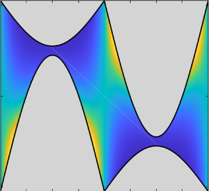
periodic in the $\theta$ direction. A typical example for this configuration space is depicted in figure 5(a).

Figure 5. Configuration space for the needle in figure 4(b) of length $\ell =2a=1$ in (a) an open channel of width $L = 1.05$; (b) a closed channel of width $L = 0.95$. ($x$ direction not shown.)

2.2.2. Closed channel

Another possibility is that $\zeta _+(\theta _i)=\zeta _-(\theta _i)$ for some set of points $\{\theta _i\}$. This breaks up $[-{\rm \pi} ,{\rm \pi} ]$ into inadmissible intervals where $\zeta _-(\theta ) > \zeta _+(\theta )$, and $N$ disjoint admissible intervals

(2.24)\begin{equation} \theta \in (\theta^{{L}}_i,\theta^{{R}}_i), \quad\text{with}\ \zeta_-(\theta) < \zeta_+(\theta), \quad i=1,\ldots,N. \end{equation}

The relevant interval is determined by the initial orientation of the swimmer. The motion of the swimmer then takes place in the configuration space

(2.25)\begin{equation} \varOmega_i = \{ (x,y,\theta) : x \in \mathbb{R},\ \zeta_-(\theta) \le y \le \zeta_+(\theta),\ \theta^{{L}}_i \le \theta \le \theta^{{R}}_i \}, \end{equation}

which is not periodic in the $\theta$ direction. A typical example for this configuration space is depicted in figure 5(b). Note that the condition $\zeta _+(\theta _i)=\zeta _-(\theta _i)$ together with the channel symmetry (2.21) implies that $\zeta _+(\theta _i + {\rm \pi})=\zeta _-(\theta _i + {\rm \pi})$.

3.1. Derivation from the stochastic differential equation

In the ABP model, the Brownian swimmer obeys the stochastic equation

(3.1a)\begin{gather} \mathrm{d}{X} = U\mathrm{d}{t} + \sqrt{2D_X}\,\mathrm{d}{W}_1, \end{gather}

(3.1b)\begin{gather}\mathrm{d}{Y} = \sqrt{2D_Y}\,\mathrm{d}{W}_2, \end{gather}

(3.1c)\begin{gather}\mathrm{d}{\theta} = \sqrt{2D_\theta}\,\mathrm{d}{W}_3, \end{gather}

in its own rotating reference frame. (We omitted any intrinsic swimmer rotation for simplicity, though this would not change the derivation appreciably. We will see that a net rotation can still emerge when the swimmer is not left–right symmetric.) In terms of absolute $x$ and $y$ coordinates, this becomes an Itô stochastic equation

(3.2a)\begin{gather} \mathrm{d}{x} = \left(U\mathrm{d}{t} + \sqrt{2D_X}\,\mathrm{d}{W}_1\right)\cos\theta - \sin\theta\,\sqrt{2D_Y}\,\mathrm{d}{W}_2, \end{gather}

(3.2b)\begin{gather}\mathrm{d}{y} = \left(U\mathrm{d}{t} + \sqrt{2D_X}\,\mathrm{d}{W}_1\right)\sin\theta + \cos\theta\,\sqrt{2D_Y}\,\mathrm{d}{W}_2, \end{gather}

(3.2c)\begin{gather}\mathrm{d}{\theta} = \sqrt{2D_\theta}\,\mathrm{d}{W}_3. \end{gather}

For now we take $U$, $D_X$, $D_Y$ and $D_\theta$ to be general functions of $(x,y,\theta ,t)$. The corresponding Fokker–Planck equation for the probability density $p(x,y,\theta ,t)$ is then

(3.3)\begin{equation} \partial_t p ={-}\boldsymbol{\nabla}\boldsymbol{\cdot}\left (\boldsymbol{U}p - \boldsymbol{\nabla}\boldsymbol{\cdot}\left (\boldsymbol{\mathsf{D}}\,p\right )\right ) + \partial_\theta^2(D_\theta\,p), \end{equation}

where , and the drift vector and diffusion tensor are respectively

(3.4)\begin{equation} \boldsymbol{U} = \begin{pmatrix} U\cos\theta \\ U\sin\theta \end{pmatrix}, \quad \boldsymbol{\mathsf{D}} = \begin{pmatrix} D_X\cos^2\theta + D_Y\sin^2\theta & \tfrac{1}{2}(D_X-D_Y)\sin2\theta \\ \tfrac{1}{2}(D_X-D_Y)\sin2\theta & D_X\sin^2\theta + D_Y\cos^2\theta \\ \end{pmatrix}. \end{equation}

See Kurzthaler, Leitmann & Franosch (Reference Kurzthaler, Leitmann and Franosch2016) and Kurzthaler & Franosch (Reference Kurzthaler and Franosch2017) for the intermediate scattering function for (3.3) in the absence of boundaries and with constant parameters.

For any fixed volume $V$ we have

(3.5)\begin{equation} \partial_t \int_V p \,\,{\mathrm{d}}V ={-}\int_V\left( \boldsymbol{\nabla}\boldsymbol{\cdot}\left (\boldsymbol{U}p - \boldsymbol{\nabla}\boldsymbol{\cdot}\left (\boldsymbol{\mathsf{D}}\,p\right )\right ) - \partial_\theta^2(D_\theta\,p) \right)\,{\mathrm{d}}V \nonumber\\ ={-}\int_{\partial V}\boldsymbol{f}\boldsymbol{\cdot} \,{\mathrm{d}}{\boldsymbol{S}}, \end{equation}

where $\partial V$ is the boundary of $V$, and the flux vector is

(3.6)\begin{equation} \boldsymbol{f} = \boldsymbol{U}p - \boldsymbol{\nabla}\boldsymbol{\cdot}\left (\boldsymbol{\mathsf{D}}\,p\right ) - \hat{\boldsymbol{\theta}}\,\partial_\theta(D_\theta\,p). \end{equation}

Thus, on the impermeable parts of the boundary we require the no-flux condition

(3.7)\begin{equation} \boldsymbol{f} \boldsymbol{\cdot} \boldsymbol{n} = 0, \quad \text{on}\ \partial V, \end{equation}

where $\boldsymbol {n}$ is normal to the boundary.

3.2. Infinite channel geometry

The previous section applies to any geometry and general $\boldsymbol {U}$, $\boldsymbol{\mathsf{D}}$, and $D_\theta$, which can be functions of $(x,y,\theta ,t)$. For our problem, these only depend on $\theta$. In an infinite channel geometry (§ 2.2), which we consider in this paper, we can eliminate the along-channel direction $x$ by defining the marginal probability density

(3.8)\begin{equation} \bar{p}(y,\theta,t) = \int_{-\infty}^\infty p(x,y,\theta,t)\,{\mathrm{d}}x. \end{equation}

In order for $\bar{p}$ to be finite, $p$ has to decay fast enough as $\lvert x \rvert \rightarrow \infty$; we use this assumption to discard some terms after we integrate (3.3) from $x=-\infty$ to $\infty$, and find an equation for $\bar{p}$

(3.9)\begin{equation} \partial_t \bar{p} ={-}\partial_y\left (U\sin\theta\,\bar{p}\right ) + \partial_y^2\left (D_{yy}\,\bar{p}\right ) + \partial_\theta^2\left (D_\theta\,\bar{p}\right ), \end{equation}

where from (3.4) $D_{yy} = [\boldsymbol{\mathsf{D}}]_{22} = D_X\sin ^2\theta + D_Y\cos ^2\theta$. For the rest of the paper we take $U$, $D_X$, $D_Y$ and $D_\theta$ to be constants, so that (3.9) simplifies to

(3.10)\begin{equation} \partial_t \bar{p} ={-} U\sin\theta\,\partial_y\bar{p} + D_{yy}(\theta)\,\partial_y^2\bar{p} + D_\theta\,\partial_\theta^2\bar{p}. \end{equation}

(Note that, instead of defining $\bar{p}$ as in (3.8), we could assume that $p$ is independent of $x$, in which case $p$ is a density per unit length that satisfies (3.10).) Equation (3.10) is our main focus. The corresponding flux vector (3.6) reduces to

(3.11)\begin{equation} \bar{\boldsymbol{f}} = (U\sin\theta\,\bar{p} - D_{yy}(\theta)\,\partial_y\bar{p})\,\hat{\boldsymbol{y}} - D_\theta\,\partial_\theta\bar{p}\,\hat{\boldsymbol{\theta}}. \end{equation}

For the channel geometry, the domain can be characterized by $\zeta _-(\theta ) < y < \zeta _+(\theta )$, so the normal vector is

(3.12)\begin{equation} \bar{\boldsymbol{n}} = \zeta_\pm'(\theta)\,\hat{\boldsymbol{\theta}} - \hat{\boldsymbol{y}}. \end{equation}

The no-flux boundary conditions on (3.10) comes from (3.7)

(3.13)\begin{equation} \bar{\boldsymbol{f}}\boldsymbol{\cdot}\bar{\boldsymbol{n}} ={-}(U\sin\theta\,\bar{p} - D_{yy}(\theta)\,\partial_y\bar{p}) - \zeta_\pm'(\theta)\,D_\theta\,\partial_\theta\bar{p} = 0, \quad y = \zeta_\pm(\theta). \end{equation}

For convenience, we gather together the main (3.10) and its no-flux boundary condition (3.13) for an infinite channel geometry

(3.14a)\begin{gather} \partial_t \bar{p} + U\sin\theta\,\partial_y\bar{p} - D_{yy}(\theta)\,\partial_y^2\bar{p} - D_\theta\,\partial_\theta^2\bar{p} = 0, \quad \zeta_-(\theta) < y < \zeta_+(\theta), \end{gather}

(3.14b)\begin{gather}U\sin\theta\,\bar{p} - D_{yy}(\theta)\,\partial_y\bar{p} + \zeta_\pm'(\theta)\,D_\theta\,\partial_\theta\bar{p} = 0, \quad y = \zeta_\pm(\theta). \end{gather}

As discussed in § 2, the domain in $\theta$ is $[-{\rm \pi} ,{\rm \pi} ]$ (periodic) for $\zeta _-(\theta ) < \zeta _+(\theta )$, which means the swimmer can fully reverse direction in the channel (open-channel configuration, figure 5a). If $\zeta _-(\theta ) \le \zeta _+(\theta )$, the domain ‘pinches off’ whenever $\zeta _-(\theta ) = \zeta _+(\theta )$, and consists of two or more disconnected pieces (closed-channel configuration, figure 5b).

5.1. Open channel

For the open-channel configuration space as described in § 2.2.1, $w(\theta )$ and $\nu (\theta )$ are $2{\rm \pi}$-periodic. The boundary condition on $\mathcal {Q}(\theta )$ is that it be periodic as well. Choosing $\theta ^{{L}}=-{\rm \pi}$ in (5.4), we have

(5.5)\begin{equation} \mathcal{Q}(-{\rm \pi}) = c_1 = \mathcal{Q}({\rm \pi}) = c_1\,\left (1 - c_2\, F({\rm \pi})\right )\,\mathrm{e}^{\varPhi({\rm \pi})}. \end{equation}

We solve for $c_2$ in (5.5) to obtain

(5.6)\begin{equation} c_2 = \left (1 - \mathrm{e}^{-\varPhi({\rm \pi})}\right ) / F({\rm \pi}), \end{equation}

and

(5.7)\begin{equation} \mathcal{Q}(\theta) = c_1\,\mathrm{e}^{\varPhi(\theta)} \left ( 1 - \left (1 - \mathrm{e}^{-\varPhi({\rm \pi})}\right ) {F(\theta)}/{F({\rm \pi})} \right ). \end{equation}

The constant $c_1$ is chosen to enforce the normalization of $\mathcal {P} = w\mathcal {Q}$

(5.8)\begin{equation} \int_{-{\rm \pi}}^{\rm \pi}\int_{\zeta_-(\theta)}^{\zeta_+(\theta)} \bar{p}_0(\theta,y)\,{\mathrm{d}}y\,{\mathrm{d}}\theta = \int_{-{\rm \pi}}^{\rm \pi} \mathcal{P}(\theta)\,{\mathrm{d}}\theta = 1. \end{equation}

If $\varPhi (\theta )$ happens to be $2{\rm \pi}$-periodic, then we have $\varPhi ({\rm \pi} )=0$, so $c_2=0$ and

(5.9)\begin{equation} \mathcal{Q}(\theta) = c_1\,\mathrm{e}^{\varPhi(\theta)}, \quad (\varPhi(\theta)\ 2{\rm \pi}\text{-periodic}). \end{equation}

The invariant probability density in this case satisfies detailed balance (Pavliotis Reference Pavliotis2014). In fact $\varPhi (\theta )$ is periodic for the very important case of a left–right symmetric swimmer, for then we have $\zeta _+(\theta ) = -\zeta _-(-\theta )$, which follows from symmetries (2.18) and (2.21). This leads to $\varDelta (-\theta ) = -\varDelta (\theta )$ and the integrand of (5.4) is odd in $\theta$. Choosing $\theta ^{{L}}=-{\rm \pi}$ then gives $\varPhi (-{\rm \pi} )=\varPhi ({\rm \pi} )=0$, i.e. $\varPhi$ is periodic.

From $\mathcal {Q}$, we can reconstruct the full invariant density from (4.4) as $\bar{p}_0(\theta ,y) = \mathcal {Q}(\theta )\,\mathrm {e}^{\sigma (\theta )y}$, with $\sigma (\theta ) = U\sin \theta /D_{yy}(\theta )$. The exponential term reflects the accumulation near both walls, as observed in experiments and simulations. The thickness of the boundary layer is $D_{yy}/U\sin \theta$, which agrees qualitatively with the results for a spherical swimmer in Elgeti & Gompper (Reference Elgeti and Gompper2013) and Ezhilan & Saintillan (Reference Ezhilan and Saintillan2015). A typical invariant density in an open-channel configuration is shown in figure 7(a) for a needle swimmer. The marginal invariant probability density $\mathcal {P}(\theta )$ is plotted in figure 8(a) for elliptical swimmers with different velocities $U$ and centres of rotation $X_{{rot}}$. From figure 7, the invariant marginal density in $y$ peaks near both walls, but not exactly at the walls, in accordance with the simulations in the appendix of Ezhilan & Saintillan (Reference Ezhilan and Saintillan2015).

Figure 7. Invariant density $\bar{p}_0 = \mathcal {Q}(\theta )\,\mathrm {e}^{\sigma (\theta )\,y}$ for $U=1$ and $D_X=D_Y=0.1$ for the needle in figure 4(b) of length $\ell =2a=1$ in (a) an open channel of width $L = 1.05$; (b) a closed channel of width $L = 0.95$, for the domain $\varOmega _1$ in figure 5(b).

Figure 8. For an ellipse with $a=2b=1/2$, $D_X=D_Y=0.1$, $D_\theta =0.01$, $U=1$, in a channel of width $L=1.2$: (a) marginal invariant probability density $\mathcal {P}(\theta )$; (b) $1/\mathcal {P}$, normalized to unit area (see (6.8) for definition of $\tau _{{rev}}$).

What is the meaning of non-zero $c_2$? It represents an average rotational drift of the needle's stochastic angle $\theta (t)$. To see this, note that in the equilibrium state we have the expectation

(5.10)\begin{equation} \mathbb{E}\mu(\theta(T)) = \int_{-{\rm \pi}}^{\rm \pi} \mu(\theta)\,\mathcal{P}(\theta)\,{\mathrm{d}}\theta = \int_{-{\rm \pi}}^{\rm \pi} (\mathcal{P}'(\theta) + c_2)\,{\mathrm{d}}\theta = 2{\rm \pi} c_2, \end{equation}

since $\mu \,\mathcal {P} - \mathcal {P}' = c_2$ and $\mathcal {P}(\theta )$ is periodic. Hence, the average rate of angular rotation of the swimmer is $\omega = 2{\rm \pi} c_2$. From (5.4), the periodic average of $\mu (\theta )$ is

(5.11)\begin{equation} \bar{\mu} = \frac{1}{2{\rm \pi}} \int_{-{\rm \pi}}^{\rm \pi} \mu(\theta)\,{\mathrm{d}}\theta = \frac{1}{2{\rm \pi}} \int_{-{\rm \pi}}^{\rm \pi} \frac{\nu(\theta)}{w(\theta)}\,{\mathrm{d}}\theta = \frac{\varPhi({\rm \pi})}{2{\rm \pi}} = \frac{1}{2{\rm \pi}} \log(1 - c_2 F({\rm \pi}))^{{-}1}, \end{equation}

which is zero if and only if $c_2=0$ ((5.6)).

Example 5.1 (invariant density for fast needle swimmer)

It is in general quite challenging to get closed-form solutions for the invariant density of a swimmer, but it can be done in the large-$U$ limit. From (5.4) and (4.18) we have

(5.12)\begin{equation} \varPhi(\theta) = \int_{-{\rm \pi}}^\theta \mu(\vartheta)\,{\mathrm{d}}\vartheta -\log w(\theta) + \text{const.}, \end{equation}

and so the leading-order invariant marginal density $\mathcal {P}=c_1w\,\mathrm {e}^\varPhi$ for a left–right-symmetric swimmer is

(5.13)\begin{equation} \mathcal{P}(\theta) = \bar{c}_1\,\exp\left (\int_{-{\rm \pi}}^\theta \mu(\vartheta)\,{\mathrm{d}}\vartheta\right ), \end{equation}

with $\bar{c} _1$ a normalization constant. For large $U$, the constant $\bar{c} _1$ can be determined by approximating the normalization integral using the maxima of $\mu$.

We illustrate this here for the needle swimmer of examples 2.1 and 4.1. For large $U$, we can approximate $\coth \varDelta \approx \textrm {sgn}(\theta )$ for $\mu = \mu _{{needle}}$ in (4.21), and we have

(5.14)\begin{equation} \mu(\theta) \approx{-} \sigma(\theta)\cos\theta\, \left (a - X_{{rot}}\right ), \quad U \rightarrow \infty, \end{equation}

with $\sigma$ defined in (4.4), and $a = \ell /2$ the needle half-length. Note that the channel width $L$ does not appear in (5.14) at leading order in large $U$: the needle spends most of its time stuck to one of the walls, so the channel width is not important. We can integrate (5.14) and use the result in (5.13) to find

(5.15)\begin{equation} \mathcal{P}(\theta) = \bar{c}_1\exp\left ( \beta\, \log\left ( \alpha\sin^2\theta + \cos^2\theta \right )^{1/(1-\alpha)}\right ), \end{equation}

with

(5.16)

We can see that ‘large $U$’ in non-dimensional terms means large $\beta$, which is a Péclet number that accounts for the position of the centre of rotation: $\beta$ is maximized when the centre of rotation is at the rear ($X_{{rot}}=-a$), which is a rear-rotating swimmer. We can now use Laplace's method to find the normalization constant $\bar{c} _1$. The maxima of the argument of the exponential in (5.15) correspond to the zeros of $\mu$ at $\theta =0$ and ${\rm \pi}$ (with $-a \le X_{{rot}} < a$). We thus find

(5.17)\begin{equation} \mathcal{P}(\theta) = \sqrt{\frac{\beta}{4{\rm \pi}}}\, \left ( \alpha\sin^2\theta + \cos^2\theta \right )^{\beta/(1 - \alpha)}, \quad \beta \gg 1. \end{equation}

In the limit $\alpha =1$ (equal diffusivities), (5.17) simplifies to

(5.18)\begin{equation} \mathcal{P}(\theta) = \sqrt{\frac{\beta}{4{\rm \pi}}}\,\mathrm{e}^{-\beta\sin^2\theta}, \quad \beta \gg 1. \end{equation}

Note that the limit $\alpha \rightarrow 0$ in (5.17) is well defined and gives $\mathcal {P}(\theta ) = \sqrt {\beta /4{\rm \pi} }\, \lvert \cos \theta \rvert ^{2\beta }$. However, the limit $\alpha \rightarrow \infty$ gives an improperly normalized density, indicating that the limits $\beta$, $\alpha \rightarrow \infty$ do not commute. (The quartic term in a Taylor series expansion of the $\log$ in (5.15) has coefficient proportional to $\alpha$, and cannot be neglected when applying Laplace's method.)

In figure 9 we compare a numerical solution for $\mathcal {P}$ to the large-$U$ form (5.17).

Figure 9. For a needle with $\ell =1$, $U=8$, $D_X=0.1$, $D_Y=1$, $D_\theta =0.01$, in a channel of width $L=1.2$ ($\beta =3.6$): (a) marginal invariant probability density $\mathcal {P}(\theta )$ (solid) and large-$U$ form (5.17) (dashed). Notice the discrepancy near $\theta =0,{\rm \pi}$, which goes away for large $U$. (b) Value of $1/\mathcal {P}$, normalized to unit area, for the same parameters.

There is some discrepancy near $\theta =0,{\rm \pi}$, which comes from the approximation (5.14) breaking down near those points, but the difference vanishes as $U$ gets larger. We also plot $1/\mathcal {P}$, which we shall need in § 6, for which the approximation is uniformly much better.

Example 5.2 (invariant density for fast circular swimmer)

When the swimmer is perfectly circular, putting $e=0$ in (4.20) gives $\mu (\theta ) = X_{{rot}}\,\sigma (\theta )\cos \theta$, which is the same as (5.14) with $a=0$ in the previous example, except that here this expression is exact. The invariant density thus has the form (5.15), with $\beta = -UX_{{rot}}/2D_Y$, which can have either sign. For $\beta \gg 1$ we recover (5.17) and (5.18) – the circular swimmer tends to align parallel to the wall. For $-\beta \gg 1$ the maxima of $\int \mu \,{\mathrm {d}}\theta$ switch from $\{0,{\rm \pi} \}$ to $\pm {\rm \pi}/2$, and we get instead of (5.17)

(5.19)\begin{equation} \mathcal{P}(\theta) = \sqrt{\frac{\lvert\beta\rvert}{4{\rm \pi}\alpha}}\, \left ( \sin^2\theta + \alpha^{{-}1}\cos^2\theta \right )^{-\lvert\beta\rvert/(1 - \alpha)}, \quad -\beta \gg 1, \end{equation}

which for $\alpha =1$ simplifies to

(5.20)\begin{equation} \mathcal{P}(\theta) = \sqrt{\frac{\lvert\beta\rvert}{4{\rm \pi}}}\,\exp({-\lvert\beta\rvert\cos^2\theta}), \quad -\beta \gg 1. \end{equation}

Comparing the latter to (5.18), we can see that fast front-rotating circular swimmers ($X_{{rot}}>0$) collect at $\theta =\pm {\rm \pi}/2$, swimming towards the wall, rather than aligning parallel to the wall. The limit $\alpha \rightarrow 0$ in 5.19 gives $\mathcal {P}(\theta ) = \tfrac 12\left (\delta (\theta - {\rm \pi}/2) + \delta (\theta + {\rm \pi}/2)\right )$.

5.2. Closed channel

For a closed-channel configuration space, as described in § 2.2.2, the domain is given by $\varOmega _i$ in (2.25), for some fixed $i$. Now the boundary condition is that there be no net flux in the $\theta$ direction, so the constant $c_2=0$ in (5.2). The solution for the invariant density is thus

(5.21)\begin{equation} \mathcal{Q}(\theta) = c_1\,\mathrm{e}^{\varPhi(\theta)}, \quad \theta^{{L}}_i \le \theta \le \theta^{{R}}_i, \end{equation}

with $c_1$ obtained by the normalization condition for $\mathcal {P} = w\mathcal {Q}$

(5.22)\begin{equation} \int_{\theta^{{L}}_i}^{\theta^{{R}}_i} \int_{\zeta_-(\theta)}^{\zeta_+(\theta)} \bar{p}_0(\theta,y)\,{\mathrm{d}}y\,{\mathrm{d}}\theta = \int_{\theta^{{L}}_i}^{\theta^{{R}}_i} \mathcal{P}(\theta)\,{\mathrm{d}}\theta = 1. \end{equation}

A typical invariant density in a closed-channel configuration is shown in figure 7(b) for a needle swimmer.

6.1. Solving the MET equation

To solve (6.1), define ${T} = w\tau '$ which satisfies

(6.2)\begin{equation} (\nu/w)\, {T} + {T}' ={-}w, \quad {T} = w\tau', \end{equation}

where $w(\theta )$ and $\nu (\theta )$ are defined in (4.10). Use the integrating factor $\tilde {c}_1\,\mathrm {e}^{\varPhi (\theta )}$ from (5.4) to get

(6.3)

where $\tilde {\mathcal {P}}(\theta ) = \tilde {c}_1\,w\,\mathrm {e}^{\varPhi }$ is analogous to the invariant density for a closed channel (5.21) and $\mathcal {C}$ is an integration constant. We choose $\tilde {c}_1$ so that the normalization condition (5.22) is satisfied: $\tilde {G}(\theta ^{{R}}) = 1$; hence, $\tilde {G}(\theta )$ is the equilibrium probability of finding the swimmer between $\theta ^{{L}}$ and $\theta$, if the channel were closed. The MET $\tau$ has a unique maximum at $\theta =\theta _*$ with $\mathcal {C} = \tilde {G}(\theta _*)$.

Now integrate (6.3)

(6.4)\begin{equation} \tau(\theta) = \int_{\theta^{{L}}}^{\theta} \frac{1}{\tilde{\mathcal{P}}(\vartheta)} \left ( \mathcal{C} - \tilde{G}(\vartheta)\right ) \,{\mathrm{d}}\vartheta, \end{equation}

which satisfies the left boundary condition $\tau (\theta ^{{L}})=0$. The right boundary condition then requires $\tau (\theta ^{{R}}) = 0$, which fixes the integration constant

(6.5)\begin{equation} \mathcal{C} = \left.\int_{\theta^{{L}}}^{\theta^{{R}}} \frac{\tilde{G}(\vartheta)}{\tilde{\mathcal{P}}(\vartheta)}\,{\mathrm{d}}\vartheta \right/ \int_{\theta^{{L}}}^{\theta^{{R}}} \frac{\,{\mathrm{d}}\vartheta}{\tilde{\mathcal{P}}(\vartheta)}. \end{equation}

Equations (6.4) and (6.5) give the MET for a swimmer starting at $\theta$ and exiting at either $\theta ^{{L}}$ or $\theta ^{{R}}$. We now focus on a particular version of this mean exit time with a more natural interpretation – the MRT.

6.2. Mean reversal time

The MRT $\tau _{{rev}}$ (or turnaround time (Holcman & Schuss Reference Holcman and Schuss2014)) is the expected time for a swimmer initially oriented with $\theta =0$ to reverse direction to $\theta =\pm {\rm \pi}$. It can be obtained from (6.4) by setting $-\theta ^{{L}}=\theta ^{{R}}={\rm \pi}$ and $\theta =0$

(6.6)\begin{equation} \tau_{{rev}} = \tau(0) = \int_{-{\rm \pi}}^0 \frac{1}{\tilde{\mathcal{P}}(\vartheta)} \left ( \mathcal{C} - \tilde{G}(\vartheta)\right ) \,{\mathrm{d}}\vartheta. \end{equation}

In Appendix A we show how the constant $\mathcal {C}$ can be eliminated to obtain

(6.7)\begin{equation} \tau_{{rev}}= \frac{\tilde{G}(0)}{1 + \mathrm{e}^{{\rm \pi}\bar{\mu}}} \int_{-{\rm \pi}}^0\frac{\,{\mathrm{d}}\vartheta}{\tilde{\mathcal{P}}(\vartheta)} + \tanh({\rm \pi}\bar{\mu}/2) \int_{-{\rm \pi}}^0 \frac{\tilde{G}(\vartheta)}{\tilde{\mathcal{P}}(\vartheta)} \,{\mathrm{d}}\vartheta, \end{equation}

where $\bar {\mu }$ is defined in (5.11). For a left–right-symmetric swimmer, $\tilde {\mathcal {P}}=\mathcal {P}$, $\bar {\mu } = 0$ and $\tilde {G}(0)=1/2$ by symmetry, so we obtain the compact expression

(6.8)\begin{equation} \tau_{{rev}} = \frac14 \int_0^{\rm \pi} \frac{\,{\mathrm{d}}\theta}{\mathcal{P}(\theta)}. \end{equation}

Example 6.1 (MRT with diffusion only)

In the absence of swimming ($U=0$), we have $\nu = 0$ from (4.10b), and $\tilde {\mathcal {P}} = \mathcal {P} = c_1w$, with $c_1^{-1} = \int _{-{\rm \pi} }^{\rm \pi} w \,{\mathrm {d}}\theta$. Hence, (6.8) is

(6.9)\begin{equation} \tau_{{rev}} = \frac{1}{2}\, \left (\int_0^{\rm \pi} w(\theta) \,{\mathrm{d}}\theta\right ) \left (\int_0^{\rm \pi} \frac{\,{\mathrm{d}}\theta}{w(\theta)}\right ). \end{equation}

For a needle with wall distance function (2.8), we get from (2.20)

(6.10)\begin{equation} w(\theta) = \zeta_+(\theta) - \zeta_-(\theta) = L - \ell\,\lvert\sin\theta\rvert \end{equation}

where $X_{{rot}}$ drops out: the centre of rotation is immaterial in the absence of swimming. We can then easily compute the integral (6.9) to obtain

(6.11)

The ‘narrow exit’ limit corresponds to $\lambda = 1 - \delta$, with $\delta$ small

(6.12)\begin{equation} \tau_{{rev}} = \frac{{\rm \pi}({\rm \pi} - 2)}{\sqrt{2\delta}} + {O}(\delta^0), \quad \delta \ll 1. \end{equation}

This is similar but not identical to Holcman & Schuss's result (Holcman & Schuss Reference Holcman and Schuss2014, (5.13))

(6.13)\begin{equation} \tau_{{rev}} = \frac{{\rm \pi}({\rm \pi}-2)}{\sqrt{2\delta}}\, \sqrt{\frac{D_Y}{2L^2D_\theta}}, \end{equation}

valid as $\delta \rightarrow 0$, but otherwise unconstrained. In figure 10, a comparison to a finite-element numerical solution of the full PDE (i.e. without using the reduced equation) shows excellent agreement with our small-$D_\theta$ form (6.11), but less so with the form (6.13). Possibly there is a parameter regime where (6.13) shows better agreement.

Figure 10. MRT for a needle as a function of $D_\theta$, for $\lambda =0.9$, $D_Y=1$. The dashed line is (6.11), which is technically valid for small $D_\theta$ but applies over a wide range. The dotted line is from Holcman & Schuss (Reference Holcman and Schuss2014). The solid line is from a finite-element simulation of the full PDE.

For an elliptical shape (2.16) with $U=0$, we have

(6.14)\begin{equation} w(\theta) = L\,(1 - \lambda\sqrt{1 - e^2\cos^2\theta}). \end{equation}

Then

(6.15)\begin{equation} L^{{-}1}\int_0^{\rm \pi} w(\theta)\,{\mathrm{d}}\theta = {\rm \pi}- 2\lambda E(e), \end{equation}

where $E$ is a complete elliptic integral of the second kind. We also have

(6.16)\begin{align} \int_0^{\rm \pi}\frac{L\,{\mathrm{d}}\theta}{w(\theta)} = \frac{\rm \pi}{\sqrt{(1 - \lambda^2)(1 - (1 - e^2)\lambda^2)}} - \frac{2}{\lambda}K(e) + \frac{2}{\lambda (1 - \lambda^2)}\, \Pi\left (\frac{e^2}{1 - \lambda^{{-}2}}\,\middle|\,e\right ), \end{align}

where $K$ and $\Pi$ are the complete elliptic integrals of the first and third kinds. Together, the product of (6.15) and (6.16) into (6.9) gives the reversal time for an ellipse. The MRT for a needle is compared to different ellipses in figure 11.

Figure 11. MRT $\tau _{{rev}}$ for a needle and different ellipses, as a function of gap size $\delta$. An ellipse reverses more rapidly as it becomes more circular, since it spends less time aligning with the wall.

6.3. Asymptotics of MRT

The integrand in (6.8) is the inverse of $\mathcal {P}(\theta ) = c_1 w(\theta )\,\mathrm {e}^{\varPhi (\theta )}$. The integral itself will thus typically be dominated by the minima of $\mathcal {P}$, which correspond to values of $\theta$ that the swimmer finds difficult to cross when trying to reverse. This could be because $\delta = 1-\ell /L$ is small: this is the narrow escape problem discussed by Holcman & Schuss (Reference Holcman and Schuss2014) (see example 6.1). However, for a swimmer the long reversal time is usually due to a swimmer ‘sticking’ to the top or bottom wall for long times.

To approximate the integral in (6.8), we look for minima $\theta _*$ of $\mathcal {P}(\theta )$, where we can approximate

(6.17)\begin{equation} \mathcal{P}(\theta) = \mathcal{P}(\theta_*)\, \exp({C_*\xi^2 + {O}(\xi^3)}), \quad \xi = \theta - \theta_*. \end{equation}

This gives us the approximation

(6.18)\begin{equation} \tau_{{rev}} \approx \frac{1}{4\mathcal{P}(\theta_*)} \int_{-\infty}^\infty \mathrm{e}^{{-}C_*\xi^2}\,{\mathrm{d}}\vartheta = \frac{1}{4\mathcal{P}(\theta_*)}\,\sqrt{\frac{\rm \pi}{C_*}} . \end{equation}

This should be multiplied by the number of minima with value $\mathcal {P}(\theta _*)$ in $0 \le \theta < {\rm \pi}$, should there be more than one. We can easily obtain a more accurate, if messier, approximation by retaining higher-order terms in (6.17).

Example 6.2 (MRT for a fast needle swimmer)

An ideal example for the asymptotic approximation of $\tau _{{rev}}$ is the fast needle swimmer of example 5.1. Figure 9(b) clearly shows strong peaks in $1/\mathcal {P}$ at $\theta _* = \pm {\rm \pi}/2$ even for this modest value of $U$. Hence, we are justified in expanding around the minimum of (5.17) at $\theta _*={\rm \pi} /2$, which gives

(6.19)\begin{equation} \mathcal{P}(\theta_*) = \sqrt{\frac{\beta}{4{\rm \pi}}}\,\alpha^{\beta/(1-\alpha)}, \quad C_* = \beta/\alpha. \end{equation}

Recall that $\alpha = D_X/D_Y$ is the ratio of diffusivities, and $\beta$ is a large Péclet number defined in (5.16). Inserting these in (6.18), we find

(6.20)\begin{equation} \tau_{{rev}}\approx \frac{\rm \pi}{2\beta}\,\alpha^{\frac12 - \frac{\beta}{1-\alpha}}, \end{equation}

or in the case $\alpha =1$

(6.21)\begin{equation} \tau_{{rev}} \approx \frac{\rm \pi}{2\beta}\,\mathrm{e}^{\beta}, \quad \alpha = 1. \end{equation}

This is exponential in the Péclet number $\beta$, so that the reversal time can become extremely long. Note also that the MRT is independent of the channel width $L$ in this limit. For the parameters in figure 9 ($\beta =3.6$), the numerical MRT is $\tau _{{rev}} \approx 1.54\times 10^3$, whereas the approximation (6.20) gives $1.38 \times 10^3$. The approximation is thus reasonably good even for a modest Péclet number $\beta$.

7.1. Homogenized equation

Rewrite the Fokker–Planck (3.3) as

(7.1)\begin{equation} \partial_t p + \partial_x(u\,p) + \partial_y(v\,p) = \partial_x^2(D_{xx}\,p) + 2\partial_x\partial_y(D_{xy}\,p) + \partial_y^2(D_{yy}\,p) + \partial_\theta^2(D_\theta\,p), \end{equation}

where $\boldsymbol {U} = (u,v)$. In this section we only assume that $\boldsymbol{\mathsf{D}}$, $D_\theta$ and $\boldsymbol {U}$ do not depend on $x$. (The derivation could easily be extended to allow $x$ dependence.) Later (§ 7.2) we will specialize to the forms in (3.4), which are functions of $\theta$ only.

We will homogenize in the $x$ direction only, since the swimmer is confined between walls in the $y$ direction and the $\theta$ direction is periodic. We introduce a large scale $x/\eta$ and long time $t/\eta ^2$, where $\eta$ is a small expansion parameter. After rescaling $t \rightarrow t/\eta ^2$ and $x \rightarrow x/\eta$, (7.1) becomes

(7.2a)\begin{equation} \mathcal{L}\,p ={-} \eta\,\partial_x(u\,p) + 2\eta\,\partial_x\partial_y(D_{xy}\,p) - \eta^2\partial_t p + \eta^2\,\partial_x^2(D_{xx}\,p), \end{equation}

where we defined the linear operator

(7.2b)

The no-flux boundary conditions for (7.2a) are

(7.2c)\begin{equation} \left (v\,p - \partial_y(D_{yy}\,p) - \eta\,\partial_x(D_{xy}\,p)\right ) + \zeta_\pm'(\theta)\,\partial_\theta(D_\theta\,p) = 0, \quad y = \zeta_\pm(\theta). \end{equation}

We expand the probability density $p$ as a regular series in $\eta$

(7.3)\begin{equation} p = p_0 + \eta\,p_1 + \eta^2\,p_2 + \ldots. \end{equation}

Define the cell integral of $f(\theta ,y)$ as

(7.4)

To ensure uniqueness at each order, we enforce the cell-integrated probability $\left \langle p \right \rangle = \left \langle p_0 \right \rangle$, so that $\left \langle p_i \right \rangle = 0$ for $i>0$.

Now we collect powers of $\eta$ in (7.2) with the expansion (7.3). At leading order in $\eta$ we have from (7.2a)

(7.5a)\begin{equation} \mathcal{L}\,p_0 = 0, \end{equation}

with boundary conditions from (7.2c)

(7.5b)\begin{equation} v\,p_0 - \partial_y(D_{yy}\,p_0) + \zeta_\pm'(\theta)\,\partial_\theta(D_\theta\,p_0) = 0, \quad y = \zeta_\pm(\theta). \end{equation}

The operator $\mathcal {L}$ only involves $(\theta ,y)$, so we can solve (7.5) with

(7.6)\begin{equation} p_0 = {P}(x,t)\,\rho(\theta,y), \quad \mathcal{L}\rho = 0, \quad \left \langle \rho \right \rangle = 1, \end{equation}

where $\rho (\theta ,y)$ is the cell-normalized $x$-independent invariant density for (7.1), and so $\left \langle p_0 \right \rangle = {P}(x,t)$.

At order $\eta ^1$, (7.2a) gives

(7.7)\begin{equation} \mathcal{L}\,p_1 ={-} \partial_x(u\,p_0) + 2\partial_x\partial_y(D_{xy}\,p_0) \nonumber\\ = \left ( - u\,\rho + 2\partial_y(D_{xy}\,\rho) \right )\,\partial_x{P}. \end{equation}

We can solve this by letting

(7.8)\begin{equation} p_1 = \chi\,\partial_x{P}, \end{equation}

where $\chi (\theta ,y)$ satisfies the cell problem

(7.9a)\begin{gather} \mathcal{L}\,\chi ={-} u\,\rho + 2\partial_y(D_{xy}\,\rho), \end{gather}

(7.9b)\begin{gather}0 = v\,\chi - \partial_y(D_{yy}\,\chi) + \zeta_\pm'(\theta)\,\partial_\theta(D_\theta\,\chi) - D_{xy}\,\rho, \quad y = \zeta_\pm(\theta), \end{gather}

with $\left \langle \chi \right \rangle =0$. The solvability condition for the cell problem (7.9) demands

(7.10)\begin{equation} \left \langle u\,\rho \right \rangle = \left \langle \partial_y(D_{xy}\,\rho) \right \rangle. \end{equation}

In our case, the left and right sides of (7.10) vanish separately after using the channel symmetry $\rho (\theta +{\rm \pi} ,y) = \rho (\theta ,-y)$. On the left, we have $u(\theta ) = U\cos \theta$, so $u(\theta +{\rm \pi} ) = -u(\theta )$ and the integral must vanish. On the right, we have $D_{xy}(\theta ) = \tfrac 12(D_X-D_Y)\sin 2\theta$ from (3.4), so $D_{xy}(\theta +{\rm \pi} ) = D_{xy}(\theta )$ and $\partial _y\rho (\theta +{\rm \pi} ,y) = -(\partial _y\rho )(\theta ,-y)$ and the integral again vanishes. There is thus no ‘ratchet effect’ to cause a net drift, since there is no breaking of the left–right symmetry of the channel. Having patterned walls as in Yariv & Schnitzer (Reference Yariv and Schnitzer2014) and Malgaretti & Stark (Reference Malgaretti and Stark2017) would likely cause such a drift.

At order $\eta ^2$, (7.2) gives

(7.11a)\begin{gather} \mathcal{L}\,p_2 ={-} \partial_x(u\,p_1) + 2\partial_x\partial_y(D_{xy}\,p_1) - \partial_t p_0 + \partial_x^2(D_{xx}\,p_0), \end{gather}

(7.11b)\begin{gather}0 = \left (v\,p_2 - \partial_y(D_{yy}\,p_2) - \partial_x(D_{xy}\,p_1)\right ) + \zeta_\pm'(\theta)\,\partial_\theta(D_\theta\,p_2), \quad y = \zeta_\pm(\theta). \end{gather}

The solvability condition then yields the effective heat equation

(7.12)\begin{equation} \partial_t {P} = D_{{eff}}\,\partial_x^2{P}, \end{equation}

where the effective diffusivity in $x$ is

(7.13)\begin{equation} D_{{eff}}=\left \langle D_{xx}\,\rho \right \rangle - \left \langle u\,\chi \right \rangle + \left \langle \partial_y(D_{xy}\chi) \right \rangle. \end{equation}

The solvability condition (7.10) implies that $\chi$ only affects the effective diffusivity up to an additive multiple of $\rho$.

7.2. Reduced equation limit

We solve the cell problem (7.9) in the same small-$D_\theta$ limit as in § 4. Anticipating that the effective diffusivity should diverge as $\varepsilon =D_\theta$ becomes smaller, we expand

(7.14)\begin{equation} \chi = \varepsilon^{{-}1}\,\chi_0 + \chi_1 + \varepsilon\,\chi_2 + \ldots. \end{equation}

The leading-order $\varepsilon ^{-1}$ cell problem (7.9) is the same as (4.3), with solution

(7.15)\begin{equation} \chi_0(\theta,y) = {X}(\theta)\, \mathrm{e}^{\sigma(\theta)y}. \end{equation}

At next order $\varepsilon ^0$ we have the PDE and boundary conditions

(7.16a)\begin{gather} U\sin\theta\,\partial_y\chi_1 - D_{yy}(\theta)\,\partial_y^2\chi_1 = \partial_\theta^2\chi_0 - \left (U\cos\theta - 2\sigma D_{xy}\right )\,\mathcal{Q}(\theta)\,\mathrm{e}^{\sigma(\theta)y}; \end{gather}

(7.16b)\begin{gather}U\sin\theta\,\chi_1 - D_{yy}(\theta)\,\partial_y\chi_1 ={-}\zeta_\pm'(\theta)\,\partial_\theta\chi_0 + D_{xy}\,\mathcal{Q}(\theta)\,\mathrm{e}^{\sigma(\theta)y}, \quad y=\zeta_\pm(\theta), \end{gather}

where we used the invariant density $\bar{p}_0 = \mathcal {Q}(\theta )\,\mathrm {e}^{\sigma (\theta )y}$. Integrate (7.16a) from $y=\zeta _-$ to $\zeta _+$ and use the boundary conditions (7.16b)

(7.17)\begin{equation} \partial_\theta(\nu{X} - w\,\partial_\theta{X}) ={-}\varXi\,\mathcal{P}, \end{equation}

where $\mathcal {P} = w\mathcal {Q}$, and

(7.18)

with $\alpha = D_X/D_Y$ as in (5.17). We integrate (7.17) once

(7.19)

with $d$ a constant of integration. The solvability condition (7.10) ensures that $H(\theta )$ is a periodic function of $\theta$. Next use the integrating factor $\mathrm {e}^{\varPhi (\theta )}$ from (5.4), with $\theta ^{{L}}=-{\rm \pi}$

(7.20)\begin{equation} w\,\mathrm{e}^{\varPhi}\,\partial_\theta(\mathrm{e}^{-\varPhi}{X}) = H(\theta) - d. \end{equation}

We integrate again and find

(7.21)\begin{equation} \mathrm{e}^{-\varPhi(\theta)}\,{X}(\theta) - {X}(-{\rm \pi}) = \int_{-{\rm \pi}}^\theta\frac{H(\vartheta)}{w(\vartheta)\,\mathrm{e}^{\varPhi(\vartheta)}} \,{\mathrm{d}}\vartheta - c_1d\,F(\theta), \end{equation}

where we used $F(\theta )$ from (5.4). By rearranging and using (5.7), we find after introducing new constants

(7.22)\begin{equation} {X}(\theta) = \tilde{c}_1\,\mathrm{e}^{\varPhi(\theta)} \left (\int_{-{\rm \pi}}^\theta\frac{H(\vartheta)}{\tilde{\mathcal{P}}(\vartheta)} \,{\mathrm{d}}\vartheta - d_2 F(\theta) \right ) + d_1\mathcal{Q}(\theta), \end{equation}

where we used $\tilde {\mathcal {P}} = \tilde {c}_1w\,\mathrm {e}^{\varPhi }$ as in § 6.1. The constant $d_1$ is adjusted to satisfy $\left \langle \chi \right \rangle =0$ and is immaterial to the effective diffusivity. The constant $d_2$ is used to enforce periodicity of ${X}$ and can be eliminated to obtain

(7.23)\begin{equation} {X}(\theta) = \tilde{c}_1\,\mathrm{e}^{\varPhi(\theta)} \left ( \int_{-{\rm \pi}}^\theta\frac{H(\vartheta)}{\tilde{\mathcal{P}}(\vartheta)} \,{\mathrm{d}}\vartheta - \frac{F(\theta)}{F({\rm \pi})} \int_{-{\rm \pi}}^{\rm \pi}\frac{H(\vartheta)}{\tilde{\mathcal{P}}(\vartheta)} \,{\mathrm{d}}\vartheta \right ) + d_1\mathcal{Q}(\theta). \end{equation}

In this reduced limit, the effective diffusivity (7.13) is

(7.24)

to leading order in $D_\theta$. The expected value $\mathbb{E}D _{xx}$ is taken over the invariant marginal density $\mathcal {P}(\theta )$, and $D_{{enh}}$ is the ‘enhanced’ part of the diffusivity.

7.3. Bounding $D_{{eff}}$ by $\tau _{{rev}}$ for a left–right-symmetric swimmer

Since the expressions are getting a bit complicated, for the sake of brevity we will focus on the left–right-symmetric case for this section. In that case the term involving $F(\theta )$ vanishes in (7.23), and $\tilde {c}_1\,\mathrm {e}^{\varPhi }$ becomes $\mathcal {Q}$

(7.25)\begin{equation} {X}(\theta) = \mathcal{Q}(\theta) \int_{-{\rm \pi}}^\theta\frac{H(\vartheta)}{\mathcal{P}(\vartheta)} \,{\mathrm{d}}\vartheta + d_1\mathcal{Q}(\theta). \end{equation}

After restoring in (7.25) the definition of $H$ from (7.19), it can be shown that the enhanced diffusivity $D_{{enh}}$ in (7.24) can be written as

(7.26)\begin{equation} D_{{enh}} = 4\int_0^{{\rm \pi}/2}\varXi(\theta)\,\mathcal{P}(\theta)\int_0^\theta \varXi(\theta')\,\mathcal{P}(\theta') \int_\theta^{{\rm \pi} - \theta} \frac{\,{\mathrm{d}}\theta''}{\mathcal{P}(\theta'')} \,{\mathrm{d}}\theta'\,{\mathrm{d}}\theta. \end{equation}

To derive this we used the symmetries $\varXi (\theta + {\rm \pi}) = \varXi ({\rm \pi} - \theta ) = -\varXi (\theta )$, $\mathcal {P}(\theta + {\rm \pi}) = \mathcal {P}({\rm \pi} - \theta ) = \mathcal {P}(\theta )$, the latter holding for a left–right-symmetric swimmer. Rearranging the inner-most integral in (7.27) gives us

(7.27)\begin{equation} D_{{enh}} = \frac12\tau_{{rev}} (\mathbb{E}\lvert\varXi\rvert)^2 - 8\int_0^{{\rm \pi}/2}\varXi(\theta)\,\mathcal{P}(\theta)\int_0^\theta \varXi(\theta')\,\mathcal{P}(\theta)' \int_0^\theta \frac{\,{\mathrm{d}}\theta''}{\mathcal{P}(\theta'')} \,{\mathrm{d}}\theta'\,{\mathrm{d}}\theta, \end{equation}

where the MRT $\tau _{{rev}}$ was defined in (6.8). The expected value in (7.27) is taken over the invariant marginal density $\mathcal {P}(\theta )$, as in (7.24).

Since $\varXi (\theta )$ defined by (7.18) is non-negative in $[0,{\rm \pi} /2]$, (7.27) immediately gives us the bound

(7.28a)\begin{equation} D_{{enh}} \le \tfrac12\tau_{{rev}}(\mathbb{E}\lvert\varXi\rvert)^2 \le \tfrac12\tau_{{rev}}\,\max_\theta \varXi^2(\theta), \end{equation}

with

(7.28b)\begin{equation} \max_{0 \le \theta \le {\rm \pi}/2} \varXi(\theta) = \begin{cases} U, & \alpha \ge 1/2; \\ U/\sqrt{4\alpha(1 - \alpha)}, & \alpha < 1/2. \end{cases} \end{equation}

This useful bound allows us to estimate $D_{{enh}}$ from $\tau _{{rev}}$, which is simpler to compute ((6.8)). The estimate tends to improve the longer the swimmer spends aligned with the walls (figure 12).

Figure 12. Effective diffusivity from (7.24) for an ellipse with $a=1$, $b=1/2$, $D_X=D_Y=0.1$, $D_\theta =0.01$, in a channel of width $L=1.2$. The dashed lines are the bound $\tfrac 12U^2\tau _{{rev}}$ from (7.28), with $\alpha =1$ and $\tau _{{rev}}$ given by (6.8). The decrease in exponential rate as the centre of rotation $X_{{rot}}$ is moved forward is similar to the asymptotic form of $\tau _{{rev}}$ for a needle, (6.21), with $\beta$ given by (5.16).