2. Flexural-gravity wavemaker problem

The wavemaker problem represents the response of a fluid-filled domain with a free surface subject to the small amplitude oscillatory motion of a vertical wall along which an arbitrary velocity distribution is imposed. It is a crucial problem and forms the basis for all eigenfunction matching methods in a finite depth fluid domain. A flexural-gravity wavemaker problem can physically be thought of as an equivalent problem when the free surface is covered with an elastic plate. When the depth of the fluid domain extends to infinity, the solution process depends on an integral of a function very similar to eigenfunctions for finite depth domain. In this section, the flexural-gravity wavemaker is considered for both finite and infinite water depths assuming linearized water wave theory and small amplitude response. The physical problem is considered in the two-dimensional Cartesian coordinate system. The fluid is assumed to be inviscid and incompressible, and the flow is irrotational and simple harmonic in time with angular frequency $\omega$ which ensures the existence of a velocity potential $\varPhi (x,y,t)$ of the form $\varPhi (x,y,t) = \textrm {Re}\{\phi (x,y)\,\textrm {e}^{-\textrm {i}\omega t}\}$. We follow the assumption that the $x$-axis is horizontal and the $y$-axis is vertically downward positive. The fluid region in the case of finite depth is the semi-infinite strip $0< x < \infty$ and $0 < y < h$, whilst for infinite depth is the quarter plane $0 < x < \infty$ and $0< y <\infty$. The spatial velocity potential $\phi (x,y)$ satisfies the partial differential equation

(2.1)\begin{equation} \nabla^2\phi = 0, \quad \mbox{in the fluid domain.} \end{equation}

On the structural boundary, the spatial velocity potential $\phi (x,y)$ satisfies the boundary condition as given by (as in Schulkes et al. Reference Schulkes, Hosking and Sneyd1987)

(2.2)\begin{equation} \left(D\frac{{\partial}^{4}}{{\partial}{x}^{4}}+Q\frac{{\partial}^{2}}{{\partial}{x}^{2}}+1-\gamma g K\right)\frac{{\partial}{\phi}}{{\partial}{y}}+K\phi=0\quad {\rm at}\ y=0,\quad 0 < x < \infty, \end{equation}

where $D=EI/{\rho }g$, $Q=N/{\rho }g$, $K=\omega ^{2}/g$, $E$ is Young's modulus, $I=d^{3}/12(1-\nu )$, $d$ is plate thickness, $\nu$ is Poisson's ratio, $N$ ($\textrm {Newton}\ \textrm {m}^{-1}$) is uniform compressive stress, $\rho$ is water density, $\gamma =\rho _i d/(\rho g)$, $g$ is the gravitational constant and $\rho _i$ is the density of the plate. It may be noted that the ice is routinely broken from stress forming ice ridges and ice keel. Therefore, the stress in compressed ice must be very high in such cases and the same high stress is considered for the study. The rigid bottom boundary (for finite depth)/no flux and boundedness (for infinite depth) condition(s) is/are given by

(2.3)\begin{equation} \left.\begin{array}{ll@{}} \phi_{y}=0 \mbox{ on } y=h & \mbox{in the case of finite depth,}\\ \phi,\mid\boldsymbol{\nabla}\phi\mid\rightarrow 0 \mbox{ as } y \rightarrow\infty & \mbox{in case of infinite depth.} \end{array}\right\} \end{equation}

Further, on the vertical boundary at $x=0$, the velocity potential $\phi (x,y)$ satisfies the conditions given by

(2.4)\begin{equation} \phi(0,y)=u(y), \end{equation}

and

(2.5)\begin{equation} \phi_x(0,y)=v(y). \end{equation}

where $u(y)$ and $v(y)$ are the prescribed functions to be introduced later.

Finally, the far-field radiation condition is given by

(2.6)\begin{equation} \lim_{x \to \infty}\left( \frac{\partial \phi}{\partial x} - \textrm{i}k_0\phi\right)=0, \end{equation}

where $k_0$ is the wavenumber associated with the plane wave solution which satisfies the dispersion relation in $k$ as given by

(2.7)\begin{equation} H(k)=0, \end{equation}

where in finite depth

(2.8)\begin{equation} H(k)= \displaystyle\frac{k(D{k}^{4}-Q{k}^{2}+1)\tanh(kh)}{1+\gamma gk\tanh(kh)}-K, \end{equation}

and in infinite depth

(2.9)\begin{equation} H(k)= \begin{cases} \displaystyle\frac{k(D{k}^{4}-Q{k}^{2}+1)}{1+\gamma g k}-K, & \mathrm{Re}(k)>0.\\ \displaystyle\frac{-k(D{k}^{4}-Q{k}^{2}+1)}{1-\gamma g k}-K, & \mathrm{Re}(k)<0. \end{cases} \end{equation}

The unique velocity potential can be obtained with specific $u(y)$ and $v(y)$ by solving the above boundary value problem with the help of appropriate edge conditions associated with the flexible plate which depend on the nature of the physical problems under consideration (see Sahoo et al. Reference Sahoo, Yip and Chwang2001; Manam et al. Reference Manam, Bhattacharjee and Sahoo2005).

The expansion formulae will be briefly discussed in the cases of infinite and finite water depths when the dispersion relation possesses distinct roots. The dispersion relation for finite water depth is an even function of $k$. In the absence of compression, it contains two real roots of the opposite sign, infinitely many imaginary roots and four complex roots. A similar convention for the location of the roots is utilized here when the ice sheet is compressed. In the case of infinite depth, there is a branch cut on the imaginary axis, and this branch cut replaces the roots on the imaginary axis (which become dense as the depth tends to infinity). A detailed analysis of the roots’ location can be found in Squire & Dixon (Reference Squire and Dixon2000), and in appendix B of Williams (Reference Williams2006), where the movement of the complex-valued roots towards either the real or imaginary axis under specific conditions is also described. We denote the positive real root as $k_0$ and the complex roots as $\pm k_I$ and $\pm k_{II}$ where $k_{II}=\bar {k}_I$ (overbar represent complex conjugate) with $k_I$ having positive real and imaginary parts.

It is worth mentioning that the inclusion of water compressibility into the formulation changes the dispersion relation slightly and results in a conversion of some of the roots located in the imaginary axis into the real axis (Abdolali et al. Reference Abdolali, Kadri, Parsons and Kirby2018). These newly formed waves are called acoustic-gravity waves that have an oscillatory profile in the vertical direction, unlike gravity waves, which have an oscillatory profile in the horizontal direction. However, incorporating water compressibility as a part of the present problem will deviate from the primary goal of studying the scattering of flexural-gravity waves. We deem it suitable for separate treatment and is thus not attempted for the time being.

The velocity potential $\phi (x,y)$ associated with the boundary value problem (BVP) satisfying (2.1)–(2.4) and (2.6) is expressed as (see Theorem 2.4 of Manam et al. Reference Manam, Bhattacharjee and Sahoo2005)

(2.10)\begin{align} \phi(x,y)&=A_{0}\,f_{0}(y)\,\textrm{e}^{\textrm{i}k_{0}x}+A_{I}\,f_{I}(y)\,\textrm{e}^{\textrm{i}k_{I}x}+ A_{II}\,f_{II}(y)\,\textrm{e}^{-\textrm{i}k_{II}x} \nonumber\\ &\quad +\frac{2}{\rm \pi}\int_{0}^{\infty}{\frac{A(\xi)M(\xi,y)\,\textrm{e}^{-\xi x}\,\textrm{d}\xi}{\varDelta(\xi)}}, \end{align}

with

(2.11)\begin{equation} \left.\begin{gathered} \displaystyle A_n=\frac{1}{C_n}\int_{0}^{\infty}u(t)\,f_n(t)\,\textrm{d}t+ \frac{k_n}{KC_n}\left[(Q-D{k_n}^{2}){\phi}_{y}-D{\phi_{yyy}}\right]_{(x,y)=(0,0)},\\ \displaystyle A(\xi)=\int_{0}^{\infty}u(t)M(\xi,t)\,\textrm{d}t+\xi\left[(Q+D{\xi}^{2}){\phi}_{y}-D{\phi_{yyy}}\right]_{(x,y)=(0,0)}, \\ \displaystyle M(\xi,y)=\xi\left(D{\xi}^{4}+Q{\xi}^{2}+1-g\gamma K\right)\cos{\xi y}-K\sin{\xi y},\\ \displaystyle\varDelta(\xi)={\xi}^{2}{\left(D{\xi}^{4}+Q{\xi}^{2}+1-g\gamma K\right)}^{2}+K^{2},\\ \displaystyle f_n(y)=\textrm{e}^{{-}k_ny}, \quad C_{n}=\frac{H'(k_n)}{2K}\quad\mbox{for} \ n=0,I,II. \end{gathered}\right\} \end{equation}

Similarly, when the velocity potential $\phi (x,y)$ satisfies condition (2.5) instead of (2.4), $A_n$ and $A(\xi )$ in (2.10) are given by

(2.12)\begin{equation} \left.\begin{gathered} \displaystyle A_n=\frac{-\textrm{i}\epsilon_n}{C_nk_n}\left\{\int_{0}^{\infty}v(t)\,f_n(t)\,\textrm{d}t+ \frac{k_n}{K}\left[(Q-D{k_n}^{2}){\phi}_{xy}-D{\phi_{xyyy}}\right]_{(x,y)=(0,0)}\right\},\\ \displaystyle A(\xi)=\frac{-1}{\xi}\left\{\int_{0}^{\infty}v(t)M(\xi,t)\,\textrm{d}t+\xi \left[(Q+D{\xi}^{2}){\phi}_{xy}-D{\phi_{xyyy}}\right]_{(x,y)=(0,0)}\right\},\\ \epsilon_n=\begin{cases} 1 & \mbox{for } n=0,I,\\ -1 & \mbox{for } n= II. \end{cases} \end{gathered}\right\} \end{equation}

The eigenfunctions $f_n(y)\,(n=0,I,II)$ and the kernel $M(\xi ,y)$ in (2.10) satisfies the orthogonal mode-coupling relation given by Manam et al. (Reference Manam, Bhattacharjee and Sahoo2005)

(2.13)\begin{equation} \left\langle \,f_m(t), \,f_n(t)\right\rangle= \begin{cases} C_n & \mbox{for } m= n, \\ 0 & \mbox{otherwise,}\end{cases} \end{equation}

where

(2.14)\begin{align} \left\langle f_m(t),\, f_n(t)\right\rangle&= \int_{0}^{\infty}\,f_m(t)\,f_{n}(t)\,\textrm{d}t-\frac{Q}{K}\left[f_m'(t)\,f_{n}'(t)\right]_{t=0}\nonumber\\ &\quad +\frac{D}{K}\left[\,f_m'''(t)\,f_{n}'(t)+\,f_{m}'(t)\,f_{n}'''(t)\right]_{t=0}. \end{align}

Further, it can be easily derived that

(2.15)\begin{equation} \left\langle M(\xi,t), \,f_n(t)\right\rangle=0 \quad \mbox{for } n=0,I,II. \end{equation}

It may be noted that the kernel $M(\xi , y)$ satisfies various identities as mentioned in Lemma 2.5 of Mondal et al. (Reference Mondal, Mohanty and Sahoo2013). Moreover, the unknowns, $A_n$ and $A(\xi )$, can be obtained by using the orthogonal mode-coupling relation as defined in (2.13) and (2.15).

In a similar manner, the velocity potential $\phi (x,y)$ in the case of finite water depth, satisfying (2.1)–(2.4) and (2.6), is obtained as

(2.16)\begin{equation} \phi(x,y)=A_{0}\,\textrm{e}^{\textrm{i}k_{0}x}\,f_{0}(y)+A_I\,\textrm{e}^{\textrm{i}k_{I}x}\,f_{I}(y)+A_{II}\,\textrm{e}^{-\textrm{i}k_{II}x}\,f_{II}(y)+\sum_{n=1}^{\infty}{A_{n}\,f_{n}(y)\,\textrm{e}^{{-}k_{n}x}}, \end{equation}

with

(2.17)\begin{equation} \left.\begin{gathered} \displaystyle A_n=\frac{1}{C_n}\int_{0}^{h}u(t)\,f_n(t)\,\textrm{d}t+ \frac{k_n\tanh{k_nh}}{KC_n}\left[(Q-D{k_n}^{2}){\phi}_{y}-D{\phi_{yyy}}\right]_{(x,y)=(0,0)},\\ \displaystyle C_{n}=\frac{H'(k_n)\tanh{k_n h}}{2K}\quad \mbox{for}\ n=0,I,II,1,2\ldots\quad\mbox{and}\quad k_n=\textrm{i}k_n, \quad\mbox{for}\ n=1,2,3,\ldots \end{gathered}\right\} \end{equation}

and the eigenfunctions

(2.18)\begin{equation} f_n(y)= \begin{cases} \displaystyle \frac{\cosh{k_n(h-y)}}{\cosh{k_nh}} & n=0,I,II.\\ \displaystyle \frac{\cos{k_n(h-y)}}{\cos{k_nh}} & n=1,2,3,\ldots,\end{cases} \end{equation}

Similarly, when the velocity potential $\phi (x,y)$ satisfies (2.5) instead of (2.4), the constants $A_n$ in (2.16) are obtained as

(2.19)\begin{equation} \left.\begin{gathered} \displaystyle A_n=\frac{-\textrm{i}\delta_n}{C_nk_n}\left\{\int_{0}^{h}v(t)\,f_n(t)\,\textrm{d}t+ \frac{k_n\tanh{k_nh}}{K}\left[(Q-D{k_n}^{2}){\phi}_{xy}-D{\phi_{xyyy}}\right]_{(x,y)=(0,0)}\right\},\\ \delta_n=\begin{cases} 1 & \mbox{for } n=0,I, 1,2,\ldots\\ -1 & \mbox{for } n=II. \end{cases} \end{gathered}\right\} \end{equation}

The orthogonal mode-coupling relation (see Manam et al. Reference Manam, Bhattacharjee and Sahoo2005) is given by

(2.20)\begin{align} \left\langle\, f_m(t),\, f_n(t)\right\rangle&= \int_{0}^{h}\,f_m(t)\,f_{n}(t)\,\textrm{d}t- \frac{Q}{K}\left[\,f_m'(t)\,f_{n}'(t)\right]_{t=0}\!+\!\frac{D}{K}\left[\,f_m'''(t)\,f_{n}'(t)+\,f_{m}'(t)\,f_{n}'''(t)\right]_{t=0},\nonumber\\ &= \begin{cases} C_n & m=n, \\ 0 & \mbox{otherwise.}\end{cases} \end{align}

The unknown coefficients, $A_n$, are also can be determined from the prescribed boundary conditions and the orthogonal mode-coupling relation defined in (2.20). Moreover, it may be noted that the orthogonal mode-coupling relation for wave–structure interaction problems in water of finite depth was initially defined by Sahoo et al. (Reference Sahoo, Yip and Chwang2001). Various other characteristics of the eigensystem and convergence of the expansion formulae in both the cases of water of finite and infinite water depths have been discussed in Sahoo (Reference Sahoo2012) and Mandal et al. (Reference Mandal, Sahoo and Chakrabarti2017). Moreover, in the above-mentioned expansion formula, it is assumed that the eigenvalues, $k_n$, are distinct roots of the dispersion relation (2.7) in both the cases of water of finite as well as infinite depths.

At this point, we would like to emphasize the influence of the plate compression on wave propagation by examining the dispersion relation provided in (2.7). Without loss of generality, the case of finite water depth is taken into account and plotted for four different values of plate compression – $Q/\sqrt {D}=1.3$, 1.75, 1.95, 2, 2.02 and $2.04$ along with the case of no compression ($Q=0$) to highlight the effect. A result for the particular approximation due to negligible inertial effect ($\gamma =0$) is also presented in the graphs using the dotted curves. The physical parameter values used for the computational purpose are the same as provided in Meylan & Squire (Reference Meylan and Squire1994) and are mentioned here for convenience: Young's modulus $E=5$ GPa, Poisson's ratio $\nu =0.3$, water density $\rho =1025\ \textrm {kg}\ \textrm {m}^{-3}$, ice density $\rho _i=922.5\ \textrm {kg}\ \textrm {m}^{-3}$, ice thickness $d=1$ m and the gravitational constant $g=9.81\ \textrm {m}\ \textrm {s}^{-2}$. The nature of the graph, which is monotonically increasing for the uncompressed plate, evolves to produce optima with an increasing value of compression. The maximum occurring for higher frequency and lower wavenumber corresponds to the primary blocking. On the contrary, the minimum occurring for lower frequency and higher wavenumber is termed the secondary blocking point (see figure 1). At both these points, the group velocity (or the slope of the $k-\omega$ curve) vanishes so that the energy propagation is zero. The dispersion relation possesses three positive real roots for any frequency between the primary and secondary blocking frequencies. With the increase in plate compression, the frequency band for having three real roots widens. One interesting observation is the occurrence of a sharp corner in the dispersion curve when $Q=2\sqrt {D}$ due to discontinuity in the group velocity $({\textrm {d}\omega }/{\textrm {d}k})$ at that point. In terms of physical interpretation, the wave envelope is broken into two parts travelling in opposite directions – a phenomenon termed as ‘buckling’, representing physically the breaking of the plate. We briefly discuss the plate buckling. Under compression, a finite plate will buckle (small perturbations will grow) for a length-dependent function of compression. It is such a factor which determines the strength of columns under compression. For an infinite plate, the buckling will occur for any compression. In our case, there is an extra term due to the hydrostatic pressure (which acts to restore the plate to equilibrium), and this means that, even for an infinite plate, there is a critical compression before bucking occurs. A further increase in the compression splits the buckling point into two parts, and they will move away from each other along the wavenumber axis. We also note that Kerr (Reference Kerr1983) has established a dependency between the vanishing of phase velocity and the mechanical failure due to buckling of the flexible plate. There will be a wavenumber band that widens with respect to an increasing compression and, in which no flexural-gravity wave can propagate irrespective of the incident wave frequency. A similar observation was also pointed out earlier by Das et al. (Reference Das, Sahoo and Meylan2018b).

Figure 1. The evolution of dispersion graphs in finite water depth as plate compression increases is shown for six different values, namely $Q=1.3\sqrt {D}$, $Q=1.75\sqrt {D}$, $Q=1.95\sqrt {D}$, $Q=2\sqrt {D}$, $Q=2.02\sqrt {D}$ and $Q=2.04\sqrt {D}$, of compression juxtaposing with the uncompressed plate ($Q=0$). The dotted curves are for the case when the inertial effect is ignored, whereas the rigid curves represent the inclusion of inertial effect. Ice thickness is kept at $d=1$ m. The generation of primary and secondary blocking points and the point of buckling are visible. As we increase the compression above $2\sqrt {D}$, the point of buckling splits and starts moving along the $k$ axis. The wavenumber band between the buckling points does not attribute to any wave propagation irrespective of any incoming frequency. The change in the dispersion curve due to the inertial effect is rather much less.

We further demonstrate the effect of plate thickness on the blocking points in figure 2 with $d=1$ m, $1.2\ \textrm {m}, \ldots ,1.5\ \textrm {m}$ and $\gamma =0$ (i.e. ignoring the inertial term with $d=1$ m). The value of compressive stress is kept fixed at $1.75\sqrt {D}$. The movement of the blocking points is visible as plate thickness increases. The action of ice thickness is to shift the blocking frequency as well as wavenumber (both primary and secondary) to a lower value, consequently, the frequency band of the multiple propagating modes shifts. The change in the position of primary and secondary blocking points is sufficiently small when the cases of $\gamma =0$ and $\gamma \neq 0$ are compared. Although the thickness of sea ice alters the frequency band of blocking, the wave profile's qualitative nature remains the same. Thus the subsequent results presented in this work, except for the plate elevation, are performed with $\gamma =0$. The effect of plate thickness is demonstrated in separate graphs whenever needed.

Figure 2. Variation of blocking points for different values of ice thickness along with $\gamma =0$ (approximation due to negligible inertial effect with $d=1$) is depicted here.

The roots of the dispersion relation (2.7) are qualitatively the same in both the finite and infinite water depth cases except for the evanescent modes. These evanescent modes are purely imaginary and have an insignificant effect on the scattering process, which form a continuum in the latter case. The movement of the roots in the complex plane with increasing values of incoming wave frequencies is graphically shown in figure 3 when the plate thickness is kept fixed at $d=1$ m. As we increase the incoming wave frequency, the roots from the complex plane travel towards the real axis and merge to create the secondary blocking (see figure 3b). The merging happens for the complex roots $k_I$, $-k_{II}$ with $k_{II}$, $-k_I$, respectively, to generate the critical points $\pm k_c$ that bifurcate into real roots. In order to distinguish the newly generated real roots from the earlier complex ones, we term them as $\pm k_1$ and $\pm k_2$. Then these roots start travelling away from each other to create in total six distinct roots (see figure 3c,d). A further increase in frequency ensures a coalition of the two real roots to generate primary blocking (see figure 3e). The coalition occurs between the roots $\pm k_0$, $\pm k_2$ to create the critical points $\pm k'_c$. Finally, $\pm k'_c$ bifurcate to regenerate the complex roots $\pm k_I$, $\pm k_{II}$ back into the physical system (see figure 3f). Note that primary blocking is associated with high frequency waves having relatively smaller wavenumber compared to secondary blocking, which occurs for waves having a lower frequency and a larger wavenumber. The same analysis of the dispersion graph is conveyed through figure 4 by a one-to-one relationship with the panels of figure 3.

Figure 3. Contour plots of dispersion relation for different values of incoming wave frequencies are shown. The location of the roots are shown with the small circles which moves in the complex plane with changing frequency. (a) For one real root ($\omega =0.345\ \textrm {s}^{-1}$), (b) during secondary blocking ($\omega =0.3696\ \textrm {s}^{-1}$), (c) for three real roots ($\omega =0.39\ \textrm {s}^{-1}$), (d) for three real roots ($\omega =0.43\ \textrm {s}^{-1}$), (e) during primary blocking ($\omega =0.4512\ \textrm {s}^{-1}$), (f) for one real root ($\omega =0.465\ \textrm {s}^{-1}$) when compressive stress $Q=1.75\sqrt {D}$. (a) Prior to secondary blocking. (b) Secondary blocking point. (c) Generation of three positive and negative real roots. (d) Movement of the middle root. (e) Primary blocking point. (f) Root after primary blocking.

Figure 4. Dispersion graphs for the same set of data values taken in figure 3. (a) Prior to secondary blocking. (b) Secondary blocking point. (c) Generation of three positive and negative real roots. (d) Movement of the middle root. (e) Primary blocking point. (f) Root after primary blocking.

3. Flexural-gravity wave scattering by a crack in a floating ice sheet

In the present section, as an application of the wavemaker problem in the case of water in infinite depth, the flexural-gravity wave scattering caused by a straight line crack in an ice sheet with compression is reinvestigated. However, the solution process is discussed in both the cases of finite and infinite water depths but limiting the corresponding analysis of wave scattering for the infinite water depth only to avoid repetition. It is worth mentioning, for brevity, that closed-form solutions are obtained elegantly following the method of Evans & Porter (Reference Evans and Porter2003) in the water of finite depth through the application of Green's integral theorem. We are analysing the behaviour of different modes of wave propagation close to the blocking frequencies in water of infinite depth using the approach of Manam et al. (Reference Manam, Bhattacharjee and Sahoo2005), which was not discussed earlier. Specifically, the form for the potential function during the amalgamation of the two roots of the dispersion relation can be written with the help of the distinct roots in the given form of the velocity potentials. Various known results of physical importance available in the literature are reproduced from the analytical expressions.

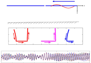
The physical domain associated with the flexural-gravity wave scattering by a crack in a floating ice sheet remains similar to that discussed in the formulation earlier in § 2 except $-\infty < x < \infty$ and $0\leqslant y < \infty$ and is exhibited in figure 5. Here, the ice sheet of thickness $d$ is modelled as two semi-infinite elastic plates separated at $x=0$ due to an open crack and floating on an undisturbed water surface $y=0$, $-\infty < x < \infty$. Further, the fluid and ice characteristics remain the same, as discussed in § 2. In the present context, we will pose the physical problem in terms of the spatial velocity potential after eliminating the spatial surface elevation $\eta (x)$ from various boundary conditions. Under the above assumptions, the spatial velocity potential satisfies Laplace equation in the fluid domain (2.1) along with the ice-covered boundary condition (2.2) and the bottom conditions (2.3).

Figure 5. Schematic diagram of a floating ice sheet having a crack.

Moreover, across the interface boundary between the two plate-covered regions, the continuity of velocity and pressure yields

(3.1)\begin{equation} {\phi}_x(0+,y)= {\phi}_x(0-,y) \quad \mbox{and}\quad {\phi}(0+,y)= {\phi}(0-,y) \quad {\mbox{in}}\ 0 < y < \infty.\end{equation}

Further, assuming the free-edge conditions (zero bending moment and shear stress) are complied with near the crack (as in Sahoo Reference Sahoo2012), the velocity potential $\phi (x,y)$ will satisfy the following relations:

(3.2)\begin{equation} B\{\phi(x,y)\}\equiv D\left[\frac{{\partial}^{2}}{{\partial}{x^2}}\left(\frac{{\partial}{\phi}}{{\partial}{y}}\right)\right]_{y=0} \rightarrow 0 \quad \mbox{ as } x \rightarrow 0 \pm , \end{equation}

and

(3.3)\begin{equation} S\{\phi(x,y)\}\equiv\left[D\frac{{\partial}^{3}}{{\partial}{x^3}}\left(\frac{{\partial}{\phi}}{{\partial}{y}}\right) +Q\frac{{\partial}^{2}\phi}{{\partial}{x}{\partial}{y}}\right]_{y=0} \rightarrow 0 \quad \mbox{ as } x \rightarrow 0 \pm. \end{equation}

The choice of free-edge conditions is made primarily because this is the most straightforward and standard boundary condition. It could be argued that under compression, other energy-conserving boundary conditions may be more appropriate (Lee & Newman Reference Lee and Newman2000; Xia, Kim & Ertekin Reference Xia, Kim and Ertekin2000; Karmakar & Sahoo Reference Karmakar and Sahoo2005; Kohout & Meylan Reference Kohout and Meylan2009). Such boundary conditions could be incorporated without any modification to the current method, but we do not do so here like this for simplicity. Finally, the velocity potential satisfies Sommerfeld's radiation boundary condition, which for one travelling wavenumber is given by

(3.4)\begin{equation} \phi(x,y)= \begin{cases} \displaystyle \frac{\textrm{i}g}{\omega}\left(\textrm{e}^{-\textrm{i}k_0x}+R_0\, \textrm{e}^{\textrm{i}k_0x}\right)\,f_0(y) & \mbox{as } x \rightarrow \infty,\\ \displaystyle \frac{\textrm{i}g}{\omega} T_0\,\textrm{e}^{-\textrm{i}k_0x}\,f_0(y) & \mbox{as } x \rightarrow -\infty, \end{cases} \end{equation}

with $k_0$ being a real root of the dispersion relations (2.7) with $R_0$ and $T_0$ being the complex constants associated with the amplitudes of the reflected and transmitted waves, respectively. However, in a system having multiple propagating modes, the above forms modify into

(3.5)\begin{equation} \phi(x,y)= \begin{cases} \displaystyle \frac{\textrm{i}g}{\omega} \left\{\left(\textrm{e}^{-\textrm{i}{\epsilon_0}k_0x}+R_0\, \textrm{e}^{\textrm{i}{\epsilon_0}k_0x}\right)\,f_0(y)+\sum_{i=1}^{p}{R_i\, \textrm{e}^{\textrm{i}{\epsilon_i}k_ix}}\,f_i(y)\right\}& \mbox{as}\ x \rightarrow \infty,\\ \displaystyle \frac{\textrm{i}g}{\omega} \sum_{i=0}^{p}{T_i\, \textrm{e}^{-\textrm{i}{\epsilon_i}k_ix}}\,f_i(y) & \mbox{as}\ x \rightarrow -\infty, \end{cases} \end{equation}

where $k_i$, $(i=0,1,\dots ,p)$ represents $(p+1)$ propagating modes which individually satisfy the radiation condition mentioned in (2.6), $R_i$ and $T_i$ are the complex constants associated with the amplitude of the reflected and transmitted waves in the $i{\mathrm {th}}$ mode and $\epsilon _i=\pm 1$ when ${\textrm {d}\omega }/{\textrm {d}k}|_{k=k_i}\gtrless 0$.

4. Method of solution

Exploiting the geometrical symmetry of the physical problem about $x=0$, the BVP defined in the half-plane in the previous section is reduced to two quarter plane BVPs (following the reduction approach adopted in Manam et al. Reference Manam, Bhattacharjee and Sahoo2005) whose solutions are sought based on the mixed type of Fourier transform as discussed in § 2. The reduced potentials are defined as

(4.1)\begin{equation} {\varphi}(x,y)={\phi}(x,y)-{\phi}({-}x,y) \quad\mbox{and} \quad{\varUpsilon}(x,y)= {\phi}(x,y)+{\phi}({-}x,y), \quad x>0. \end{equation}

Thus, ${\varphi }(x,y)$ and ${\varUpsilon }(x,y)$ satisfy the governing equation (2.1) in the quarter plane $x>0$, $y>0$ along with the plate-covered condition (2.2) and the bottom condition (2.3) independently. Finally, the continuity conditions in (3.1) yields

(4.2)\begin{equation} {\varUpsilon}_x(x,y)=0 \quad\mbox{and} \quad{\varphi}(x,y)=0 \quad \mbox{at } x=0 , 0 < y < \infty. \end{equation}

From the continuity equation (4.2), it is clear that $\varphi (x,y)$ satisfies (2.4) and $\varUpsilon (x,y)$ satisfies (2.5) with $\varphi (0,y)=u(y)=0$ and ${\varUpsilon }_x(0,y)=v(y)=0$ for $0<y<\infty$. The edge conditions (3.2) and (3.3) for the bending moment and shear force in terms of $\varphi (x,y)$ and $\varUpsilon (x,y)$ yield

(4.3a,b)\begin{gather} D\frac{{\partial}^{2}}{{\partial}{x^2}}\left(\frac{{\partial}{\varUpsilon(0,0)}}{{\partial}{y}}\right) = 0,\quad D\frac{{\partial}^{3}}{{\partial}{x^3}}\left(\frac{{\partial}{\varUpsilon(0,0)}}{{\partial}{y}}\right)+Q \frac{{\partial}^{2}\varUpsilon(0,0)}{{\partial}{x}{\partial}{y}}=0, \end{gather}

(4.4a,b)\begin{gather} D\frac{{\partial}^{2}}{{\partial}{x^2}}\left(\frac{{\partial}{\varphi(0,0)}}{{\partial}{y}}\right) = 0, \quad D\frac{{\partial}^{3}}{{\partial}{x^3}}\left(\frac{{\partial}{\varphi(0,0)}}{{\partial}{y}}\right)+Q\frac{{\partial}^{2}\varphi(0,0)}{{\partial}{x}{\partial}{y}}=0. \end{gather}

The expansion formulae for distinct roots of the dispersion relation derived in § 2 will be applied here to derive the expression for reduced potentials in both cases of infinite and finite depth water domain.

4.1. Infinite depth water domain

Here, the reduced potential $\varphi (x,y)$ is expanded as

(4.5)\begin{align} \varphi(x,y)&=\frac{\textrm{i}g}{\omega}\left[\textrm{e}^{-\textrm{i}k_{0}x-k_{0}y}+A_{0}\,f_{0}(y)\, \textrm{e}^{\textrm{i}k_{0}x}+A_{I}\,f_{I}(y)\,\textrm{e}^{\textrm{i}k_{I}x}+A_{II}\,f_{II}(y) \,\textrm{e}^{-\textrm{i}k_{II}x}\right. \nonumber\\ &\quad \left. +\frac{2}{\rm \pi}\int_{0}^{\infty}{\frac{A(\xi)M(\xi,y)\, \textrm{e}^{-\xi x}\,\textrm{d}\xi}{\varDelta(\xi)}}\right], \end{align}

where $\varDelta (\xi )$, $M(\xi ,y)$ and the eigenfunctions $f_n(y) (n=0,I,II)$ for infinite depth are the same as defined in § 2. In between the frequency band of primary and secondary blocking, when three propagating modes exist, we denote the positive real roots as $k_0$, $k_1$ and $k_{2}$ where $k_{2}$ is the root corresponding to negative energy flux. The form of the reduced potential given by (4.5) is valid with $k_I$, $k_{II}$ replaced by $k_1$, $k_2$, respectively, and even at the time of blocking in which case either $k_1=k_2$ or $k_0=k_2$. Without loss of generality, we solve the problem with the case of complex roots $k_I$, $k_{II}$, and easily extend it to the multiple real roots $k_1$, $k_2$.

Utilizing the relation (4.2) along with the edge boundary conditions (4.4a,b) and the orthogonal property of the eigenfunctions as in (2.13) and (2.15), the unknown coefficients, $A_n$ and $A(\xi )$, are obtained as

(4.6)\begin{equation} \left.\begin{gathered} A_0=\frac{\omega}{\textrm{i}g}\frac{k_0}{KC_0}\left(Q-Dk^2_0\right){\alpha}_1-1, \quad A_I=\frac{\omega}{\textrm{i}g}\frac{k_I}{KC_I}\left(Q-Dk^2_I\right){\alpha}_1,\\ A(\xi)=\frac{\omega}{\textrm{i}g} \xi\left(Q+D{\xi}^2\right)\alpha_1, \quad {A}_{II}=\frac{\omega}{\textrm{i}g}\frac{k_{II}}{KC_{II}}\left(Q-Dk^2_{II}\right){\alpha}_1, \quad \alpha_1=\frac{2\textrm{i}k^2_0\left(Q-Dk^2_0\right)}{\beta_1},\\ \beta_1=\frac{\omega}{\textrm{i}g}\left\{\frac{\textrm{i}k^3_0}{KC_0}(Q-Dk^2_0)^2 +\frac{\textrm{i}k^3_I}{KC_I}\left(Q-Dk^2_I\right)^2-\frac{\textrm{i}k^3_{II}}{KC_{II}}\left(Q-Dk^2_{II}\right)^2\right.\\ -\left.\frac{2K}{\rm \pi}\int_{0}^{\infty}{\frac{\xi^3\left(Q+D{\xi}^2\right)^2\,\textrm{d}\xi}{\varDelta(\xi)}}\right\}. \end{gathered}\right\} \end{equation}

Proceeding in a similar manner, the reduced potential ${\varUpsilon }(x,y)$ is expressed as

(4.7)\begin{align} \varUpsilon(x,y)&=\frac{\textrm{i}g}{\omega}\left[\textrm{e}^{-\textrm{i}k_{0}x-k_{0}y}+B_{0}\,f_{0}(y)\, \textrm{e}^{\textrm{i}k_{0}x}+B_{I}\,f_{I}(y)\,\textrm{e}^{\textrm{i}k_{I}x}+B_{II}\,f_{II}(y)\,\textrm{e}^{-\textrm{i}k_{II}x}\right.\nonumber\\ &\left.\quad +\frac{2}{\rm \pi}\int_{0}^{\infty}{\frac{B(\xi)M(\xi,y)\,\textrm{e}^{-\xi x}\,\textrm{d}\xi}{\varDelta(\xi)}}\right]. \end{align}

The unknown constants $B_n$, for $n=0,I,II.$ and the unknown function $B(\xi )$ being

(4.8)\begin{equation} \left.\begin{gathered} B_0=\frac{\omega}{g}\frac{Dk^2_0}{KC_0}{\alpha}_2+1,\quad B_I=\frac{\omega}{g}\frac{Dk^2_I}{KC_I}{\alpha}_2,\quad B(\xi)={-}\frac{\omega}{\textrm{i}g}D{\xi}^2\alpha_2,\quad B_{II}={-}\frac{\omega}{g}\frac{Dk^2_{II}}{KC_{II}}{\alpha}_2,\\ \alpha_2=\frac{-2k^3_0}{\beta_2},\quad {\beta_2}=\frac{\omega}{\textrm{i}g}\left\{\frac{\textrm{i}Dk^5_0}{KC_0}+\frac{\textrm{i}Dk^5_I}{KC_I}- \frac{\textrm{i}Dk^5_{II}}{KC_{II}}+\frac{2K}{\rm \pi}\int_{0}^{\infty}{\frac{D\xi^5 \,\textrm{d}\xi}{\varDelta(\xi)}}\right\}. \end{gathered}\right\} \end{equation}

Within the frequency band of primary and secondary blocking, $k_I$ and $k_{II}$ become real valued, redefined as $k_1$ and $k_2$, respectively, with the relation $k_0<k_{2}<k_1$, and the same potential form obtained in (4.5) is valid. In the subsequent sections, all the analysis and results are shown for the case of infinite depth water domain only. However, it is deemed suitable to provide the form of the potential functions for finite depth water domain.

4.2. Finite depth water domain

The reduced potential $\varphi (x,y)$ in this case can be expressed as

(4.9)\begin{align} \varphi(x,y)&=\frac{\textrm{i}g}{\omega}\left[\vphantom{\sum_{n=1}^{\infty}}\left(\textrm{e}^{-\textrm{i}k_{0}x}+A_{0}\,\textrm{e}^{\textrm{i}k_{0}x}\right)\,f_{0}(y)+A_I\,\textrm{e}^{\textrm{i}k_{I}x}\,f_{I}(y)+A_{II}\,\textrm{e}^{-\textrm{i}k_{II}x}\,f_{II}(y)\right. \nonumber\\ &\quad \left.+\sum_{n=1}^{\infty}{A_{n}\,f_{n}(y)\,\textrm{e}^{{-}k_{n}x}}\right], \end{align}

where the eigenfunctions $f_n(y)\ (n=0,I,II,1,2,3\ldots .)$ for finite depth are the same as defined in § 2.

Using (4.2), (4.4a,b) and (2.20), the unknown coefficients, $A_n$, are obtained as

(4.10)\begin{equation} \left.\begin{gathered} A_0=\frac{\omega}{\textrm{i}g}\frac{k_0\tanh{k_0h}}{KC_0}\left(Q-Dk^2_0\right){\alpha}_1-1,\\ A_n=\frac{\omega}{\textrm{i}g}\frac{k_n\tanh{k_nh}}{KC_n}\left(Q-Dk^2_n\right){\alpha}_1, \quad \mbox{for}\ n=I,II,1,2,3,\ldots,\\ \alpha_1=\frac{2\textrm{i}k^2_0\tanh{(k_0h)}\left(Q-Dk^2_0\right)}{\beta_1}, \quad \mbox{and}\quad k_n=\textrm{i}k_n \quad \textrm{for}\ n=1,2,3,\ldots,\\ \beta_1=\frac{\omega}{\textrm{i}g}\left[\frac{\textrm{i}k^3_0\tanh^2{(k_0h)}}{KC_0}(Q-Dk^2_0)^2+ \frac{\textrm{i}k^3_I\tanh^2{(k_Ih)}}{KC_I}\left(Q-Dk^2_I\right)^2\right.\\ \quad-\left.\frac{\textrm{i}k^3_{II}\tanh^2{(k_{II}h)}}{KC_{II}}\left(Q-Dk^2_{II}\right)^2 -\sum_{n=1}^{\infty}{\frac{k^3_n}{KC_n}\left\{\left(Q+Dk^2_n\right)\tan{(k_nh)}\right\}^2}\right]. \end{gathered}\right\} \end{equation}

Likewise, the reduced potential ${\varUpsilon }(x,y)$ is expressed as

(4.11)\begin{align} \varUpsilon(x,y)&=\frac{\textrm{i}g}{\omega}\left[\vphantom{\sum_{n=1}^{\infty}}\left(\textrm{e}^{-\textrm{i}k_{0}x}+B_{0}\,\textrm{e}^{\textrm{i}k_{0}x}\right)\,f_{0}(y)+B_I\,\textrm{e}^{\textrm{i}k_{I}x}\,f_{I}(y)+B_{II}\,\textrm{e}^{-\textrm{i}k_{II}x}\,f_{II}(y) \right.\nonumber\\ &\quad \left.+\sum_{n=1}^{\infty}{B_{n}\,f_{n}(y)\,\textrm{e}^{{-}k_{n}x}}\right], \end{align}

with the unknown constants, $B_n$, obtained as

(4.12)\begin{equation} \left.\begin{gathered} B_0=\frac{\omega}{g}\frac{Dk^2_0\tanh{k_0h}}{KC_0}{\alpha}_2+1,\quad B_n=\frac{\omega}{g}\frac{Dk^2_n\tanh{k_nh}}{KC_n}{\alpha}_2,\quad \textrm{for}\ n=I,1,2,3,\ldots\\ B_{II}={-}\frac{\omega}{g}\frac{Dk^2_{II}\tanh{k_{II}h}}{KC_{II}}{\alpha}_2, \quad \alpha_2={-}\frac{2k^3_0\tanh{(k_0h)}}{\beta_2},\\ \beta_2=\frac{\omega}{\textrm{i}g}\left\{\frac{\textrm{i}k^5_0D\tanh^2{(k_0h)}}{KC_0}+ \frac{\textrm{i}k^5_ID\tanh^2{(k_Ih)}}{KC_I}-\frac{\textrm{i}k^5_{II}D\tanh^2{(k_{II}h)}}{KC_{II}}\right.\\ \quad +\left.\sum_{n=1}^{\infty}{\frac{Dk^5_n\tan^2{(k_nh)}}{KC_n}}\right\}. \end{gathered}\right\}\end{equation}

Next, we shift our focus to the case of infinite water depth in the subsequent analysis. While extending the result from complex roots $k_I$, $k_{II}$ to real roots $k_1$, $k_2$, all the notations used will also be redefined by replacing the suffices $I$, $II$ with 1, 2, respectively. Since there are three progressive wave modes present in the system, each of which travels with different group velocity, the reflection and transmission coefficients which express the transport of energy must be derived with care.

5. Energy balance relation

In the theoretical study of scattering of water waves, the energy balance relation or energy identity plays a pivotal role in the understanding of scattering of wave energy and exhibits the relation among the scattering coefficients such as the reflection and transmission coefficients. Often, the energy identity is used as a check of the computed results of these scattering coefficients. In this section, the energy identity is derived using Green's integral theorem involving the complex velocity potential and its complex conjugate. Further, the occurrence of negative group velocity in the system will be demonstrated with the derived energy identity.

To obtain the energy identity, we use Green's integral theorem, as given by

(5.1)\begin{equation} \int_{C}\left(\bar{\phi}\frac{\partial\phi}{\partial n}-\phi\frac{\partial\bar{\phi}}{\partial n}\right)\textrm{d}s=0, \end{equation}

where $C$ denotes the closed boundary of the fluid region, which is union of two closed boundary $C_1$ and $C_2$, $\bar {\phi }$ is the complex conjugate of $\phi$, which satisfies (2.1)–(2.3) and (3.1)–(3.5), and ${\partial }/{\partial n}$ represents the outward normal derivative to the closed boundary $C$. The closed boundary $C_1$ consists of the horizontal upper surface ($0<x<X$; $y=0$), vertical boundaries ($0<y<\infty$; $x=X$), bottom boundary ($0<x<X$; $y\rightarrow \infty$) and vertical boundary at the crack ($0<y<\infty$; $x=0$), and closed boundary $C_2$ consists of the horizontal upper surface ($-X<x<0$; $y=0$), vertical boundaries ($0<y<\infty$; $x=-X$), bottom boundary ($-X<x<0$; $y\rightarrow \infty$) and vertical boundary at the crack ($0<y<\infty$; $x=0$), ultimately letting $X\rightarrow \infty$.

Using the boundary conditions and the far-field radiation condition in (5.1), we obtain the energy relation as given by

(5.2)\begin{equation} K_r^2+K_t^2=1, \end{equation}

where

(5.3)\begin{equation} \left.\begin{gathered} K_r^2=\left|\frac{B_0+A_0}{2}\right|^2+\left(\frac{k_1 C_{g}(k_1)}{k_0 C_{g}(k_0)}\right)\left|\frac{B_1+A_1}{2}\right|^2-\left(\frac{k_{2} C_{g}(k_{2})}{k_0 C_{g}(k_0)}\right)\left|\frac{B_{2}+A_{2}}{2}\right|^2,\\ K_t^2=\left|\frac{B_0-A_0}{2}\right|^2+\left(\frac{k_1 C_{g}(k_1)}{k_0 C_{g}(k_0)}\right)\left|\frac{B_1-A_1}{2}\right|^2-\left(\frac{k_{2} C_{g}(k_{2})}{k_0 C_{g}(k_0)}\right)\left|\frac{B_{2}-A_{2}}{2}\right|^2 \end{gathered}\right\} \end{equation}

and

(5.4)\begin{equation} C_g(k_j)=\frac{1}{2}\sqrt{\frac{g}{k_j}}\frac{(5Dk_j^4-3Qk_j^2+1)+2k_j^3g\gamma(2Dk_j^2-Q)}{(1+k_jg\gamma)\sqrt{(1+k_jg\gamma)(Dk_j^4-Qk_j^2+1)}} \quad\mbox{for } j=0,1, 2, \end{equation}

with $k_0$ being the wavenumber associated with the incident wave.

The newly defined reflection ($K_r$) and transmission ($K_t$) coefficients are now plotted against $T=2{\rm \pi} /\omega$ in figure 6 for three values of compressive stress. It is observed that both the coefficients now have values less than one within the frequency band of primary and secondary blocking in which the dispersion relation possesses three distinct real roots (see figure 6b). Moreover, the transitions of $K_r$ and $K_t$ at the primary and secondary blocking points are also shown in figures 6(a) and 6(c), respectively, for the same values of compressive stress. A continuous transition is observed and this validates the correctness of the newly derived expressions for $K_r$ and $K_t$. We here mention that, in order to compute $K_r$ and $K_t$ outside the frequency band of primary and secondary blocking, the following formulae have been used due to the existence of only one propagating mode:

(5.5a,b)\begin{equation} K_r^2=\left|\frac{B_0+A_0}{2}\right|^2\quad\mbox{and}\quad K_t^2=\left|\frac{B_0-A_0}{2}\right|^2. \end{equation}

A similar study for three different values of plate thickness is carried out, and the results are graphically shown in figure 7. Similar observations as were made in figure 6 are made in this case as well. The only difference is observed in terms of the values of $T$ at which the primary and secondary blocking points are obtained. Corresponding primary and secondary blocking occur at higher values of $T$ as the plate thickness increases.

Figure 6. Values of $K_r$ and $K_t$ are plotted for three different values of compressive stress. Panel (a) depicts the continuity of $K_r$ and $K_t$ across primary blocking frequency. Sharp corners in the graphs are due to the blocking; $k_{I}$ is the incident wave after primary blocking. Panel (b) depicts $K_r$ and $K_t$ within the frequency band of primary and secondary blocking in which three propagating modes exist. Both the coefficient values are below one after using the modified energy relation. Panel (c) depicts the continuity of $K_r$ and $K_t$ across secondary blocking frequency; $k_{0}$ is the incident wave before secondary blocking. (a) Transition through primary blocking. (b) Within the frequency band of primary and secondary blocking. (c) Transition through secondary blocking.

Figure 7. Values of $K_r$ and $K_t$ are plotted for three different values of plate thickness. (a) Transition through primary blocking. (b) Within the frequency band of primary and secondary blocking. (c) Transition through secondary blocking.

6. Scattering process through the primary and secondary blocking points

In this section, we will discuss the scattering process due to a crack when primary and secondary blocking occur under the influence of fixed compressive stress acting on the plate. Without loss of generality, we can consider the case of secondary blocking in which any incoming frequency lower than the blocking frequency corresponds to one propagating mode, and any higher frequency generates three propagating modes. A similar process happens in the case of the primary blocking, with the only difference being the occurrence of three propagating modes at a frequency lower than that of the blocking frequency. The transition from one propagating mode to three or vice versa occurs through the blocking frequency. It is thus intuitive to say that this transition occurs continuously, and the justification follows below.

At the instance of secondary blocking, one can have $\pm k_I=\pm k_1=\pm k_{II}=\pm k_2=\pm k_c$ (see figure 8). However, the potential form (4.5) is still valid since $k_1$, and $-k_{2}$ are two different values, albeit their absolute values being the same. The potential form given by (4.5) reflects the fact that the root $k_{2}$, corresponding to the waves with negative energy flux, is taken from the negative wavenumber region (of the form $-k_{2}$). The movement of the roots of the dispersion relation in the complex plane plays a pivotal role in the scattering process through the blocking frequency. Four complex roots $\pm k_I$ and $\pm k_{II}$, and two real roots $\pm k_0$ of the dispersion relation are the possible choices of wave modes for the physical process, to begin with. Next, we look for those roots which provide a bounded solution for the scattering problem due to the crack. Hence, the roots of the form $k_0$, $k_I$, $-k_{II}$ are the suitable candidates to provide bounded solution in the region $x>0$. Consequently, even though $k_I$ merges with $k_{II}$ at the moment of secondary blocking, it is feasible to continue the process with $-k_{II}$. An equivalent choice of roots in the region $x<0$ will be $-k_0$, $-k_I$, $k_{II}$, and similarly the process may continue with $k_{II}$ when $-k_I$ merges with $-k_{II}$. In this sense, the root $-k_{II}$ is qualitatively equivalent to the root $k_{II}$ for the crack problem. As soon as the complex roots $k_I$ and $k_{II}$ merge at $k_c$, they can take the form $k_1$ and $k_2$, respectively. The same goes for their counterpart on the left side half. Following the earlier discussion of figure 3, although $k_I$, $k_{II}$ merges at $k_c$, the contribution from $k_{II}$ (equivalently $k_2$) can be obtained from $-k_{II}$ (equivalently $-k_2$). Consequently, the overlapping of the roots at the blocking points can be avoided simply by taking one root from the negative real axis. Thus, the theory for distinct roots is unequivocally applicable at the secondary blocking. A similar situation arises at the time of primary blocking where $\pm k_I=\pm k_0=\pm k_{II}=\pm k_2=\pm k'_c$. An exactly similar process but of reverse order will happen that will bifurcate $\pm k'_c$ into the complex plane to regenerate the roots $\pm k_I,\pm k_{II}$. The locus of the roots of the dispersion relation during the complete scattering process is depicted for three different values of compressive stress. The scattering process through the blocking frequency is thus smooth due to the continuous movement of the roots of the dispersion relation in the complex plane without any kind of overlapping.

Figure 8. The movement of roots of the dispersion relation with an increase in frequency is shown for different values of compressive stress $Q$. For each of the figures, the first point of simultaneous contact in the real axis for red and blue curves (roots which are travelling from the complex plane) corresponds to secondary blocking. With further increase in frequency, the roots move along the real axis in the direction as shown in the figure. Then, at the primary blocking, the red and pink curve simultaneously leave the real axis to move in the complex plane. All the three roots are distinct during the scattering process, even during blocking, unlike in the case of plane wave propagation in which root coalescence occurs. Consequently, the theory of distinct roots of the dispersion relation will work perfectly in the scattering process.

It is, however, feasible to consider any of the three propagating modes (in the frequency band of primary and secondary blocking) as the incident wave and hence the potential function can be written as

(6.6)\begin{align} \begin{pmatrix} \phi_{1r}(x,y) \\ \phi_{2r}(x,y) \\ \phi_{3r}(x,y) \end{pmatrix} &=\frac{\textrm{i}g}{\omega}\left[\begin{pmatrix} I_{00} & 0 & 0 \\ 0 & I_{01} & 0 \\ 0 & 0 & I_{02} \end{pmatrix} \begin{pmatrix} \textrm{e}^{-\textrm{i}k_0 x}\,f_0(y) \\ \textrm{e}^{-\textrm{i}k_1 x}\,f_1(y) \\ \textrm{e}^{\textrm{i}k_{2} x}\,f_{2}(y) \end{pmatrix}\right.\nonumber\\ &\quad +\overbrace{\begin{pmatrix} K_{r11} & K_{r12} & K_{r13} \\ K_{r21} & K_{r22} & K_{r23} \\ K_{r31} & K_{r32} & K_{r33} \end{pmatrix}}^{\mbox{Scattering matrix }(S_R)} \begin{pmatrix} \textrm{e}^{\textrm{i}k_0 x}\,f_0(y) \\ \textrm{e}^{\textrm{i}k_1 x}\,f_1(y) \\ \textrm{e}^{-\textrm{i}k_{2} x}\,f_{2}(y) \end{pmatrix} \left. +\frac{2}{\rm \pi}\begin{pmatrix} a\\a\\a \end{pmatrix}\right] \quad \mbox{for } x>0, \end{align}

with

(6.7)\begin{equation} a=\int_{0}^{\infty}{\frac{A(\xi)M(\xi,y)\,\textrm{e}^{-\xi x}\,\textrm{d}\xi}{\varDelta(\xi)}}, \end{equation}

and $\phi _{jr}\ (j=1,2,3)$ represents the form of the velocity potential when $k_i\ (i=0,1,2)$ is the incident wave mode, respectively. The scattering matrix, denoted by $S_R$, defines the relationship between the forward and backward moving waves ($k_0<k_{2}<k_1$). It is to be noted that the direction of the wave envelope for $k_{2}$ is opposite to that of $k_0$ and $k_1$. The $j$th row ($j=1,\,2,\,3$) of it respectively corresponds to $k_i$ as the incident wave mode ($i=0,\,1,\,2$), and the corresponding amplitude ratios of the reflected waves are ${K_{rjl}}/{I_{0i}}$ ($j,\ l=i+1$ with $i=0,\,1,\,2$) for each $i$, where $I_{0i}$ is the incident wave amplitude of the mode $k_i$ (taken to be unity in the numerical calculation). Moreover, the transmitted velocity potential can be written as

(6.8)\begin{equation} \begin{pmatrix} \phi_{1t}(x,y) \\ \phi_{2t}(x,y) \\ \phi_{3t}(x,y) \end{pmatrix}=\frac{\textrm{i}g}{\omega} \overbrace{\begin{pmatrix} K_{t11} & K_{t12} & K_{t13} \\ K_{t21} & K_{t22} & K_{t23} \\ K_{t31} & K_{t32} & K_{t33} \end{pmatrix}}^{\mbox{Scattering matrix }(S_T)} \begin{pmatrix} \textrm{e}^{-\textrm{i}k_0 x}\,f_0(y) \\ \textrm{e}^{-\textrm{i}k_1 x}\,f_1(y) \\ \textrm{e}^{\textrm{i}k_{2} x}\,f_{2}(y) \end{pmatrix} +\frac{2\textrm{i}g}{{\rm \pi}\omega}\begin{pmatrix} b\\b\\b \end{pmatrix}\quad \mbox{for } x<0 , \end{equation}

where

(6.9)\begin{equation} b=\int_{0}^{\infty}{\frac{A(\xi)M(\xi,y)\,\textrm{e}^{\xi x}\,\textrm{d}\xi}{\varDelta(\xi)}}, \end{equation}

and $\phi _{jt}\ (j=1,2,3)$ represents the form of the velocity potential when $k_i\ (i=0,1,2)$ is the incident wave mode, respectively. Here, the amplitude ratios of the transmitted waves are ${K_{tjl}}/{I_{0i}}$ for each $k_i$. The scattering matrix is denoted by $S_T$.

Outside the frequency band of primary and secondary blocking, there exists only one propagating mode, denoted by $p_0$, and it can be any of the $k_i$ values, and two complex modes $k_I$ and $-k_{II}$ for a bounded solution. Now $K_{ri}$ ($i=0,1,2$), respectively, represent the amplitude ratio of the modes $p_0$, $k_I$ and $-k_{II}$ in the reflected wave region; $K_{ti}$ is the same in the transmitted wave region. This will provide us further insight into mode conversion in terms of continuous transition of the amplitude ratio across blocking frequency. The scattering matrix is plotted against time period $T$ (${2{\rm \pi} }/{\omega }$) in figure 9. Figure 9(a,b) provides the scattering matrices assuming $k_1$ as the incident wave inside the frequency band of primary and secondary blockings. Sharp corners are occurring at the blocking frequencies. The top graph of figure 9(a) shows the continuity of $K_{r0}$ and $K_{r22}$. This means the incident wave $k_1$ remains as the only propagating mode above (or below) the primary blocking frequency (or time period). This is consistent with the root movement described earlier in figure 8 (see the blue curve) in which $k_I$ converts into the propagating mode and remains in the real axis. The middle and bottom graphs show the continuity of ($K_{r1}$, $K_{r21}$) and ($K_{r2}$, $K_{r23}$), respectively. This justifies the conversions of mode $k_0$ into $k_I$ and $k_2$ into $-k_{II}$ across the blocking frequency. These findings are consistent with figure 8 if we follow the red and pink curves, respectively. A similar pattern (figure 9b) of continuity is observed in the transmitted wave region as well. Figure 9(c) provides the mode conversion at the secondary blocking frequency when $k_0$ is being treated as the incident wavenumber. All three subplots show the continuity in amplitude ratio across the blocking frequency, namely $K_{r11}$ and $K_{r0}$, justifying the transformation of $k_0$ as the propagating mode; $K_{r12}$ and $K_{r1}$, justifying the transformation of $k_1$ into $k_I$; $K_{r13}$ and $K_{r2}$, justifying the transformation of $k_2$ into $k_{II}$. These observations are also in accordance with figure 8. An exact similar continuity of these modes in the transmitted wave region can be found in figure 9(d). Keeping the plate compression fixed, for example, $Q=1.75\sqrt {D}$, the same effect can be observed (figure 10a) when the plate thickness increases. The plate thickness only increases (or decreases) the time period (or frequency) at which the primary blocking occurs (see figure 10a,b). A similar pattern is observed at the secondary blocking point as well (figure 10c,d).

Figure 9. Amplitude ratio of different reflected and transmitted waves are plotted with time period $T$ around the primary and secondary blockings for various values of compressive stress. At secondary blocking, the curve is continuous if $k_0$ is taken as incident wave, whereas $k_I$ becomes the incident wavenumber at the primary blocking. The continuity of the graphs confirms the transformation of wave modes across blocking frequencies as claimed in the figure 8. (a) Reflected modes near primary blocking. (b) Transmitted modes near primary blocking. (c) Reflected modes near secondary blocking. (d) Transmitted modes near secondary blocking.

Figure 10. Amplitude ratio of different reflected and transmitted waves are plotted with period $T$ around the primary and secondary blockings for various values of plate thickness for a fixed plate compression $Q=1.75\sqrt {D}$. It is visible that the period (or frequency) at which both the primary and secondary blockings occur increases (or decreases) with an increase in plate thickness. (a) Reflected modes near primary blocking. (b) Transmitted modes near primary blocking. (c) Reflected modes near secondary blocking. (d) Transmitted modes near secondary blocking.

7. Plate deflection

The plate deflection ($\omega ^2\eta (x)/agk_0$) in the vertical direction is obtained from the following linearized kinematic condition:

(7.1)\begin{equation} \frac{\partial H(x,t)}{\partial t}=\frac{\partial \varPhi(x,y,t)}{\partial y} \quad \mbox{ on } y = 0, \end{equation}

where the flexural-gravity wave elevation $H(x,t)=\eta (x)\,\textrm {e}^{-\textrm {i}\omega t}$ and $a$ is the initial wave amplitude, which is kept at unity without loss of generality. The above equation yields the following form of the vertical plate deflection:

(7.2) \begin{align} \frac{\omega^2}{agk_0}\eta(x)= \begin{cases} \displaystyle \frac{1}{ak_{0}}\left[k_{0}\,\textrm{e}^{-\textrm{i}k_{0}x}+\frac{A_{0}+B_0}{2}k_{0}\, \textrm{e}^{\textrm{i}k_{0}x}+\frac{A_{I}+B_I}{2}k_{I}\,\textrm{e}^{\textrm{i}k_{I}x}\right.\\ \displaystyle \quad+\left.\frac{A_{II}+B_{II}}{2}k_{II}\,\textrm{e}^{-\textrm{i}k_{II}x}+ \frac{K}{\rm \pi} \int_{0}^{\infty}{\frac{\{B(\xi)+A(\xi)\}\xi \,\textrm{e}^{-\xi x}\,\textrm{d}\xi}{\varDelta (\xi)}}\right] & \mbox{for } x>0,\\ \displaystyle \frac{1}{ak_{0}}\left[\frac{B_{0}-A_0}{2}k_{0}\,\textrm{e}^{-\textrm{i}k_{0}x}+ \frac{B_{I}-A_I}{2}k_{I}\,\textrm{e}^{-\textrm{i}k_{I}x}\right.\\ \displaystyle \quad+\left.\frac{B_{II}-A_{II}}{2}k_{II}\, \textrm{e}^{\textrm{i}k_{II}x}+\frac{K}{\rm \pi}\int_{0}^{\infty}{\frac{\{B(\xi)-A(\xi)\}\xi \, \textrm{e}^{\xi x}\,\textrm{d}\xi}{\varDelta(\xi)}}\right] & \mbox{for }\ x < 0. \end{cases} \end{align}

The evolution of the plate deflection against spatial distance as the propagating wave modes transit through primary and secondary blocking points is depicted in figure 11 for three different plate thickness values. While figure 11(a) deals with the transition through the primary blocking point, the same at the secondary blocking point is illustrated in figure 11(b). The top subplot in figure 11(a) shows the plate profile just before the primary blocking at which an increase in the amplitude is observed around the crack at $x=0$. Otherwise, the wave profile is very regular away from the crack. The middle subplot depicts the situation when primary blocking occurs. Since the incident wave gets blocked at the primary blocking point, the wave environment gets very rough. A very high plate amplitude suggests such a concentration of wave energy throughout the plate while the regular pattern of the deflection starts deteriorating. After the primary blocking, the wave with negative energy flux starts propagating and distributes the energy among three wave modes. The superposition of three propagating wave modes makes the wave profile irregular, but the wave amplitude diminishes compared to the case when primary blocking occurs (lower subplot). It is also observed that the deflection is discontinuous in nature near the crack for all three cases (before, after and at blocking frequencies). However, the maximum amplitude is still larger than that of the case of a single propagating mode (from the visual comparison with the top subplot). The effect of the wave with negative energy flux can be seen from the deflection seen in $x<0$. When the wave packet impinges on the crack, it interacts with the wave profile on the $x>0$ region and creates a different wave profile than observed in the $x<0$ region. A further increase in $T$ (equivalently, decrease in $\omega$) creates the secondary blocking point at which the wave with negative energy flux merges with one of the propagating modes. The nature of the irregularity in the deflection profile becomes very prominent (bottom subplot of figure 11b). Since one of the waves responsible for this blocking point has negative energy flux, the ice deflection is not as high (middle subplot) as was observed in the primary blocking point. After the secondary blocking, the only remaining propagating mode has a smaller wavelength and lower frequency compared to the case when one propagating mode was observed before primary blocking. This mode does not have as significant an influence at the crack as was found before primary blocking. The values of $T$ for which the primary and secondary blockings occur increase with an increase in plate thickness, and the corresponding wave profiles get more dispersed (see the red curves corresponding to $d=1.2$ m). However, the qualitative nature of the profiles remains the same.

Figure 11. Vertical ice deflection is plotted against spatial distance for different values of ice thickness. Compressive stress $Q=1.75\sqrt {D}$ is taken for the study. (a) Evolution of ice deflection is depicted here at the primary blocking point with upper and lower subplots due to one and multiple propagating modes, respectively. (b) The same graph for the secondary blocking point.

Figure 12 illustrates the same study for different values of the compressive stress while keeping the plate thickness fixed. The pattern of the graphs is very similar that discussed for figure 11. Just like the effect of plate thickness discussed earlier, a higher value of compressive stress disperses the wave more.

Figure 12. Vertical ice deflection is plotted against spatial distance for different values of compressive stress acting on the ice. Plate thickness is kept fixed as $d=1$. (a) Evolution of ice deflection is depicted here at primary blocking point with upper and lower subplots due to one and multiple propagating modes, respectively. (b) The same graph for the secondary blocking point.