


1. Introduction
Model-scale experiments have been used for a long time in engineering to assess the performance of full-scale devices. The use of models at a laboratory scale is based on the robust theory of similarity, which states that if a problem is controlled by a certain number  $n$ of non-dimensional parameters
  $\varPi$, when these parameters have the same value at the model and at the full scale, then full-scale quantities can be fully determined using quantities obtained at the model scale. Unfortunately, this kind of perfect similarity can be hardly obtained, because of physical limitations of the laboratory apparatus. In practice, the main problem consists of the fact that some physical parameters (i.e. the gravitational acceleration, the speed of sound, the viscosity of the fluid) are nearly constant at the two scales. When perfect similarity cannot be obtained often imperfect similarity is invoked, thus ensuring equality of the most important non-dimensional groups and accepting a scale effect, namely an error when moving from the small scale to the full one. Typical examples are the problems of aerodynamics, where the force coefficients depend at least on the Reynolds number and Mach number, or problems of hydrodynamics in density-variable flows, where the force coefficients depend at least on the Froude number and Reynolds number. Among the systems evaluated in engineering applications using model-scale experiments, the performance of marine propellers is traditionally assessed through the use of model-scale experimental tests in towing tanks or in circulation channels. Such laboratories may work in the presence of the free surface and the propeller is placed at a depth that minimizes the interaction between the fluid-dynamic field and the free surface (i.e.
  $Fn=U/\sqrt (g h) \sim 0$ where
  $Fn$ is the Froude number, based on the advance velocity of the propeller and the distance
  $h$ of the propeller axis from the free surface). Typically,
  $Fn \sim 0.2 - 0.4$ is considered a working value for engineering purposes (range of values relating to cases of propellers of commercial ships) (Watson Reference Watson1998). As is well known, non-dimensional coefficients are calculated to be used for prediction of the performance at full scale. The technique is well established, based on a solid theoretical background and used for design purposes in naval engineering. Similarly, more recently, numerical simulations of the turbulent flow field around a ship's propeller are being carried out in partial replacement of laboratory tests. No matter the methodology employed, the problem is solved at
  $Fn=0$, meaning that the presence of the free surface is not considered, since it adds complications without contributing to the computation of the propeller performance.
Nowadays, requests for the prediction of the noise emitted by moving bodies at sea are becoming increasingly stringent, to satisfy rules aimed at the protection of the marine environment from acoustic pollution (DNV 2010). The issue of noise generation and propagation in the far field also concerns renewable-energy systems, such as wind turbines or hydrokinetic turbines, because of their potential environmental and biological impact. Since most of the noise emitted by these systems is associated with the rotor, the search for a compromise between performance and level of noise constitutes a challenge for the designers. The problem is further complicated by the fact that the laboratory-scale tests may not be fully indicative of the prediction of the noise at full scale, due to two main reasons: the scaling from the model to full scale which is not straightforward; and the presence of the free surface, which even at  $Fn= 0$, may have a strong impact on the far-field noise, which may contain a contribution coming from the reflection from the water–air interface.
Analysis and prediction of noise production and propagation in the far field have been subjects of intensive research since the early 1950s; theories have been developed also supported by laboratory and field experiments together with advanced numerical techniques. A comprehensive review on this topic is given in Wang, Freund & Lele (Reference Wang, Freund and Lele2006).
When computing the noise emitted by a body in relative motion in a fluid, the acoustic analogy (Lighthill Reference Lighthill1952, Reference Lighthill1954; Ffowcs-Williams & Hawkings Reference Ffowcs-Williams and Hawkings1969) is often employed, meaning that the evaluation of the acoustic field is decoupled from that of the hydrodynamic field. Once a numerical solution of the flow field around the body has been obtained, the data are processed by the acoustic solver which characterizes the noise source and calculates noise propagation in the medium. The advantage of the acoustic analogy is twofold: it allows use of a computational domain that is suitably small, limited to the fluid-dynamic source; and in low-Mach-number applications, it allows use of the incompressible-flow assumption for the evaluation of the flow field, whereas the compressibility associated with the noise propagation is accounted for in the acoustic model.
The acoustic analogy has been successfully applied in a number of applications (Najafi-Yazdi, Bres & Mongeau Reference Najafi-Yazdi, Bres and Mongeau2011; Ianniello, Muscari & Di Mascio Reference Ianniello, Muscari and Di Mascio2013; Wang & Wang Reference Wang and Wang2013; Nitzkorski & Mahesh Reference Nitzkorski and Mahesh2014; Jacob, Praveen & Mahesh Reference Keller, Kumar and Mahesh2018; Cianferra, Ianniello & Armenio Reference Cianferra, Ianniello and Armenio2019a). Among others, in Ianniello et al. (Reference Ianniello, Muscari and Di Mascio2013) and Jacob et al. (Reference Keller, Kumar and Mahesh2018) the acoustic analogy was adopted to characterize the acoustic signature of ship propellers in unbounded domains, whereas in the very recent paper by Wang, Wang & Wang (Reference Wang, Wang and Wang2021), it was used for the case of the Sevik rotor ingesting the turbulent wake of a circular cylinder placed orthogonally to the flow direction, in the incompressible-flow regime.
At the same time, cutting-edge acoustic field detection techniques have been developed recently and tested to address acoustic problems using laboratory-scale experimental devices. Among others, Felli, Falchi & Dubbioso (Reference Felli, Falchi and Dubbioso2015) performed a detailed investigation into the relation between the coherent structures present in the wake of a model-scale ship propeller and acoustic sources, through a combined use of tomographic particle image velocimetry (PIV) and Powell's acoustic analogy. Specifically, the authors showed the importance of the wake on the overall noise produced by the rotor. More recently, Alexander, Devenport & Glegg (Reference Alexander, Devenport and Glegg2017) studied the effect of ingestion of the turbulent field generated by a boundary layer on the noise propagated upstream by the Sevik rotor in the incompressible regime, for a wide range of load conditions (related to the parameter  $J$ defined in the next section) and boundary-layer thickness. The signal appeared broadbanded with significant amplitude in the range of low frequencies.
The brief literature survey is relative to numerical and physical experiments at laboratory scale. As we show in the present paper, this may introduce a scale effect due to the fact that similarity is imperfect when the data are to be used for predictions at the full scale.
Since the seminal work of Lighthill (Reference Lighthill1952), indications have been given on how to scale the acoustic pressure, or more precisely the law of proportionality of acoustic pressure with the Mach number. The classic example, known as the 8th power law (density perturbation variance  $\overline {\rho '^{2}}$ is proportional to
  $U^{8}_0$, with
  $U_0$ the velocity scale of the flow) was first estimated for a circular free jet (Lighthill Reference Lighthill1952, Reference Lighthill1954). In particular, if
  $D$ is the length scale of the flow, assuming that the time scale of large eddies in the flow is
  $D/U_0$, that the Reynolds stresses scale as
  $\rho U_0^{2}$ and the relevant volume
  $V$ is of order
  $D^{3}$, the pressure disturbance in the flow
  $p'$ associated with a density perturbation (with
  $p' = c_0^{2} \rho '$ and
  $c_0$ the speed of sound) reads
 \begin{equation} \frac{p'}{\rho_0 U_0^{2}} \sim \left(\frac{ D}{4{\rm \pi} r} \right) M_0^{2} \end{equation}
with  $r$ the source–observer distance, and
  $M_0 = U_0/c_0$.
This breakthrough result emphasized the importance of the wake in the production of the overall noise. However, the 8th power law of Lighthill comes from the dimensional analysis of the term  $\partial _{tt} T_{ij}$, which is one among the possible noise sources associated with the wake. In aeroacoustic research subsequent to Lighthill's papers, the knowledge of the scaling laws associated with the three classical acoustic sources (monopole, dipole and quadrupole) has been consolidated, in view of the formulation of Ffowcs-Williams & Hawkings (Reference Ffowcs-Williams and Hawkings1969) (FWH). The following relationships hold for compact sources:
(i) monopole
 ${p'}/{\rho _0 U_0^{2}} \sim {D}/{r}$;
(ii) dipole
${p'}/{\rho _0 U_0^{2}} \sim ({D}/{r}) M_0$;(iii) quadrupole
${p'}/{\rho _0 U_0^{2}} \sim ({D}/{r}) M_0^{2}$;


showing the different power of Mach number for the three fundamental types of sources. The error associated with the different terms, arising when the Mach similarity is not considered, has never been clearly reported in the literature. Further, it is important to highlight that the scaling laws reported above, and commonly accepted in the scientific community, refer to the terms of the FWH equation decaying as  $1/r$ only. However, although in the very far field the terms decaying as
  $1/r$ may dominate over the others, in the near-to-intermediate field the terms decaying as
  $1/r^{2}$ and
  $1/r^{3}$ may affect the resulting signal and it may be noteworthy to consider their correct scaling. This issue represents the main purpose of our work.
Specifically, in the present paper we pay attention to the general problem of rotors in the incompressible fluid-dynamic regime (low Mach number) and, without losing generality, we focus on a ship propeller. We investigate the scaling properties of all the possible sources of noise associated with the motion of a rotating rigid body in the low-Mach-number flow regime and on their own impact when considering the full-scale acoustic field as a direct derivation from model-scale measurements or computations. Further, we investigate how the presence of a reflecting free surface (namely the air–water interface), present in a large number of applications, affects the acoustic spectrum.
To quantify the error associated with imperfect scaling we consider the FWH equation because of its own richness. Indeed, it is composed of a number of terms identifying different physical mechanisms contributing to the generation and propagation of the noise. First, our analysis exploits scaling properties of these different physical mechanisms contributing to the sound propagation in order to quantify the error arising from imperfect scaling. Second, we apply the method of images to the FWH equation, to account for the presence of a reflecting free surface and analyse its own effect on the propagation of the signal. Indeed, when the FWH is adopted, for example to characterize the noise emission of a propeller behind a hull (see, among others, the recent work of Liefvendahl & Bensow Reference Bensow and Liefvendahl2016), to the best of our knowledge, the acoustic signal is calculated not considering the free surface. In the present paper we aim to estimate the possible error associated with the lack of free surface.
Although we focus on a marine propeller, the rationale is valid for any device tested at a laboratory scale (among others, wind turbines), whose acoustic performance must be evaluated together with the standard fluid-dynamic ones. It is to be noted that the direct applicability of the analysis provided here, albeit general, focuses on the case of a single-phase medium and steady outer conditions.
The flow field is not calculated from scratch, rather, we use the database of Cianferra, Petronio & Armenio (Reference Cianferra, Petronio and Armenio2019b), relative to a propeller in open sea conditions at  $Fn=0$. This is the main reason why the present paper is devoted to the analysis of a ship propeller, although the theoretical framework and the results of the analysis are of wide interest in fluid mechanics. The reference numerical solution is obtained using large eddy simulation (LES) in an unbounded domain (free surface is not present,
  $Fn=0$). For the acoustic analysis we consider the free surface as a boundary in the acoustic model. In other words, the free surface is at a distance such that hydrodynamic interactions are negligible, but acoustic reflections are not. Since the decay of the acoustic pressure level is related to the distance from the noise source, we point out how this decay can play a fundamental role when considering a reflection plane, such as that given by the free surface. The paper is organized as follows: § 2 contains the scaling analysis and shows how imperfect similarity (or scaling) may affect the quality of the signal at the full scale. Section 3.1 contains the mathematical modelling of the free surface in the acoustic model and analysis of the contribution of noise reflection on the acoustic field. Section 4 contains an analysis aimed at evaluating the total error when moving from laboratory scale to full scale, in the presence of imperfect scaling in an unbounded domain. Concluding remarks are given in § 5.
2. Scaling analysis of the FWH equation
Different methodologies have been developed in the literature to treat the integral solution of the FWH differential equation (see, among others, Di Francescantonio Reference Di Francescantonio1997; Brentner & Farassat Reference Brentner and Farassat1998; Najafi-Yazdi et al. Reference Najafi-Yazdi, Bres and Mongeau2011; Cianferra et al. Reference Cianferra, Ianniello and Armenio2019a). The presence of a uniform mean flow makes the numerical experiment herein considered comparable to a wind tunnel case. Thus, to consider the deviation of the acoustic field from the perfectly spherical one, the advective wave equation should be adopted (see e.g. Najafi-Yazdi et al. (Reference Najafi-Yazdi, Bres and Mongeau2011) or Cianferra et al. (Reference Cianferra, Ianniello and Armenio2019a)). We have compared results obtained adopting both advective and non-advective formulations, finding the differences insignificant for the purpose of this study, although the classical FWH formulation appears more streamlined and easy to handle. For this reason, we use the original FWH equation. The microphones have to be considered at rest in the fixed-to-the-body frame of reference, and the acoustic pressure waves propagate without being affected by advection.
The original FWH equation reads as
 \begin{align} \hat{p}(\boldsymbol{x},t) & = \frac{\partial}{\partial t} \int_{S} \left[ \frac{\rho v_i \hat{n}_i}{4{\rm \pi} r |1 - M_r|} \right]_{\tau} \,\textrm{d}S + \frac{1}{c_{0}} \frac{\partial}{\partial t} \int_{S} \left[ \frac{\tilde{p} \hat{n}_i \hat{r}_i}{4 {\rm \pi}r |1 - M_r|} \right]_{\tau} \,\textrm{d}S \nonumber\\ &\quad + \int_{S} \left[ \frac{\tilde{p} \hat{n}_i \hat{r}_i}{4 {\rm \pi}r^{2} |1 - M_r|} \right]_{\tau} \,\textrm{d}S + \frac{1}{c_{0}^{2}}\frac{\partial^{2}}{\partial t^{2}}\int_{W} \left[ \frac{ T_{rr} }{4 {\rm \pi}r |1 - M_r|} \right]_{\tau} \,\textrm{d}W \nonumber\\ &\quad + \frac{1}{c_{0}}\frac{\partial}{\partial t} \int_{W} \left[ \frac{3 T_{rr} - T_{ii}}{4 {\rm \pi}r^{2} |1 - M_r|} \right]_{\tau} \,\textrm{d}W + \int_{W} \left[ \frac{3 T_{rr} - T_{ii}}{4 {\rm \pi}r^{3} |1 - M_r|} \right]_{\tau} \,\textrm{d}W \end{align}
where  $T_{ij} = \rho u_{i} u_{j} + ( \tilde {p} - c_0^{2} \tilde {\rho } ) \delta _{ij}$ is the Lighthill tensor,
  $\tilde {p} = p - p_0$ denotes the pressure perturbation with respect to the reference value
  $p_0$,
  $\rho$ is the bulk density,
  $\tilde {p} - c_0^{2} \tilde {\rho }$ is the deviation from an isentropic behaviour,
  $\hat {n}$ is the (outward) unit normal vector to the surface element
  $\textrm {d}S$,
  $\textrm {d}W$ is the volume element,
  $r = | \boldsymbol {x} - \boldsymbol {y} |$ is the source–observer distance, with
  $\boldsymbol {x}$ the microphone location and
  $\boldsymbol {y}$ the integration variable,
  $\hat {r}_i$ is the
  $i$-component of the unit vector
  $(\boldsymbol {x} - \boldsymbol {y})/ r$,
  $v_i$ is the
  $i$-component of the surface velocity vector,
  $M_r = v_i \hat {r}_i /c_0$ the local Mach number in the source–observer direction, with
  $c_{0}$ the speed of sound.
The non-dimensional form of (2.1) is obtained considering the characteristic scale quantities  $U,D$ and
  $T$, namely: the advance velocity, the diameter of the propeller and its period of rotation. Note that the viscosity does not play a direct role in the propagation of the acoustic pressure, although Reynolds number effects may affect the turbulent field and indirectly the production of noise. Since the
  $Re$ similarity used for model-scale tests is imperfect, to minimize the scale effect for the evaluation of the hydrodynamic performance, tests are run at values of
  $Re$ large enough to ensure the presence of a fully developed turbulent field. The Reynolds number of the reference simulation (
 $Re \sim 10^{6}$) is similar to that of the recent simulations of Kumar & Mahesh (Reference Kumar and Mahesh2017) and Posa et al. (Reference Posa, Broglia, Felli, Falchi and Balaras2019) and to that of the experiments of Alexander et al. (Reference Alexander, Devenport and Glegg2017). At these values of
  $Re$, the near wake is characterized by a population of vortical well-organized and mutually interacting structures; the far wake, where ‘the flow field loses the memory of blade geometry…’ (Kumar & Mahesh Reference Kumar and Mahesh2017), might exhibit some Reynolds number dependence although a self-similar behaviour has been observed; overall, recent literature shows that the rotor wake may be little dependent on
  $Re$. In other words, although Reynolds number effects may be present, they are expected to be of minor importance, in particular regarding the noise production. Indeed, the large and energy-carrying scales of motion are those mostly responsible for the production of noise and these scales are present at the laboratory scale when analysing low-Mach-number rotor wakes. The scale effect on
  $Re$ is not considered in the present study, which is more focused on scaling of the acoustic properties of a flow field, and it may be a topic of future research.
We can replace the variables appearing in (2.1) as follows:
 \begin{equation} \left.\begin{gathered} u_i = u_i^{*} U, \quad r = r^{*} D, \quad \hat{p}, \, \tilde{p} = p^{*} \rho U^{2}, \quad v_n = v_n^{*} U, \\ t = t^{*} T, \quad \textrm{d}S = \textrm{d}S^{*} D^{2}, \quad \textrm{d}W = \textrm{d}W^{*} D^{3}, \end{gathered}\right\} \end{equation}
where the superscript  $*$ denotes non-dimensional quantities. Note that acoustic pressure
  $\hat {p}$ and fluid-dynamic pressure
  $\tilde {p}$ scale similarly, and the characteristic time scale, the period of rotation, is proportional to the reciprocal of the rotation frequency
  $T \sim 1/n$,
  $n$ being the number of revolutions per second.
Writing the equation in non-dimensional form we obtain
 \begin{align} p^{*} & = \frac{D}{T U} \frac{\partial}{\partial t^{*}} \int_{S^{*}} \left[ \frac{ v^{*}_i \hat{n}_i}{4 {\rm \pi}r^{*} |1 - M_r|} \right]_{\tau^{*}} \,\textrm{d}S^{*} + \frac{D}{T} \frac{1}{c_{0}} \frac{\partial}{\partial t^{*}} \int_{S^{*}} \left[ \frac{\tilde{p}^{*} \hat{n}_i \hat{r}_i}{4 {\rm \pi}r^{*} |1 - M_r|} \right]_{\tau^{*}} \,\textrm{d}S^{*} \nonumber\\ &\quad + \int_{S^{*}} \left[ \frac{\tilde{p}^{*} \hat{n}_i \hat{r}_i}{{4 {\rm \pi}r^{*}}^{2} |1 - M_r|} \right]_{\tau^{*}} \,\textrm{d}S^{*} + \frac{D^{2}}{T^{2}} \frac{1}{c_{0}^{2}}\frac{\partial^{2}}{\partial {t^{*}}^{2}}\int_{W^{*}} \left[ \frac{ T^{*}_{rr} }{4 {\rm \pi}r^{*} |1 - M_r|} \right]_{\tau^{*}} \,\textrm{d}W^{*} \nonumber\\ &\quad + \frac{D}{T} \frac{1}{c_{0}}\frac{\partial}{\partial t^{*}} \int_{W^{*}} \left[ \frac{3 T^{*}_{rr} - T^{*}_{ii}}{4 {\rm \pi}{r^{*}}^{2} |1 - M_r|} \right]_{\tau^{*}} \,\textrm{d}W^{*} + \int_{W^{*}} \left[ \frac{3 T^{*}_{rr} - T^{*}_{ii}}{{4 {\rm \pi}r^{*}}^{3} |1 - M_r|} \right]_{\tau^{*}} \,\textrm{d}W^{*}. \end{align}
 Note that the Lighthill tensor is made non-dimensional as  $T_{ij} = T^{*}_{ij} \rho U^{2}$, and the non-dimensional time delay at which the integrals must be evaluated is
  $\tau ^{*}=\tau /T$.
For the sake of clarity, the non-dimensional integral terms of (2.3) are named as follows: first surface term (thickness term)  $P^{T}$, second and third surface terms (loading terms)
  $P^{L1}$ and
  $P^{L2}$, respectively. These terms are also linear. The latter three volume or nonlinear terms are named
  $P^{V1}$,
  $P^{V2}$ and
  $P^{V3}$, respectively.
Thus, considering the advance ratio coefficient  $J = U/nD$, equation (2.3) may be re-written as
 \begin{equation} p^{*} = \frac{1}{J} P^{T} + \frac{Dn}{c_0} P^{L1} + P^{L2} + \frac{D^{2} n^{2}}{c_0^{2}} P^{V1} + \frac{Dn}{c_0} P^{V2} + P^{V3}, \end{equation}
which states that the non-dimensional acoustic pressure scales with  $J$ and the velocity ratio
  $V_r=Dn/c_0$
 \begin{equation} p^{*} = f(J,V_r) . \end{equation}
Here,  $V_r$ represents the ratio between the tangential velocity and the speed of sound and represents a bulk rotational Mach number, namely
  $V_r=J M_0$ where
  $M_0=U/c_0$.
A similar scaling is obtained using the  $\varPi$ theorem. In particular, if we use
  $\rho ,U$ and
  $D$ as repeated variables, we obtain
  $p^{*}=f(J,U/c_0)$ with
  $U/c_0=M_0=V_r/J$, which contains the same information as the scaling obtained using the FWH equation. Hereafter, we retain the scaling obtained in (2.4), even if the discussion holds for the similar scaling shown above. In hydrodynamics, considering the case of a ship propeller, laboratory-scale tests aimed at reproducing a full-scale quantities are performed using Froude
  $F_n$ and
  $J$ similarity, implying
 \begin{equation} F_{n_m} = \frac{U_m}{\sqrt{g D_m}} = \frac{U_f}{\sqrt{g D_f}} = F_{n_f} \quad \mbox{and}\quad J_m = \frac{U_m}{n_m D_m} = \frac{U_f}{n_f D_f} = J_f , \end{equation}
where the subscripts  $m$ and
  $f$ denote model-scale and full-scale variables, respectively. Once the scale factor is defined as
  $D_f = \lambda D_m$, we obtain
 \begin{equation} U_f = \sqrt{\lambda} U_m \quad \mbox{and}\quad n_f = n_m / \sqrt{\lambda}. \end{equation}
These conditions can be easily set to give the thrust and torque coefficients to be used at full scale, once the scale effect related to imperfect scaling for the Reynolds number has been minimized. Applying this similarity to the acoustic field leads to
 \begin{equation} \frac{D_m n_m}{c_0} = \frac{1}{\sqrt{\lambda}} \, \frac{D_f n_f}{c_0}, \end{equation}
which means that the similarity expressed in (2.4) is imperfect once the speed of sound has the same order of magnitude at the real scale and at the laboratory scale  $c_0=c_{0_f} \sim c_{0_m}$. Indeed, this is the case in typical laboratory experiments carried out using water. The similarity would become perfect if we considered
  $c_{0_m} = c_{0_f} / \sqrt {\lambda }$, and this can be easily satisfied in numerical computations. Regarding the term
  $1/|1 - M_r|$ appearing in all integral kernels, we observe that maximum values are obtained when
  $\boldsymbol {v}$ and
  $\boldsymbol {r}$ are parallel to each other, giving
  $1/|1 - |\boldsymbol {v}|/c_0|$. For underwater or in general in low-Mach-number applications, when considering perfect or imperfect similarity this value slightly varies around unity. Regarding the treatment of the time delays in the integrals above, we recall the maximum frequency parameter (
 $MFP$) introduced by Cianferra et al. (Reference Cianferra, Ianniello and Armenio2019a). Once the microphone location and the integration domain of the FWH equation have been established, this parameter rules the maximum frequency that can be captured correctly, without calculating time delays. Hence, it gives a limiting frequency below which the assumption
  $t = \tau$ is valid. We recall that, in order to avoid computation of the time delays, which makes unaffordable the direct evaluation of the volume terms (see Cianferra et al. Reference Cianferra, Ianniello and Armenio2019a),
  $MFP = 1/\varDelta _{del} f_{max} > 1$, with
 \begin{equation} \varDelta_{del} = \frac{\displaystyle\max_{\boldsymbol{y} \in S_p} | \boldsymbol{y} - \boldsymbol{x}_{mic} | - \min_{\boldsymbol{y}\in S_p} | \boldsymbol{y} - \boldsymbol{x}_{mic} | }{c_0}, \end{equation}
and  $f_{max}$ the highest frequency at which the fluid-dynamic process is observed. Note that, if
  $dt$ is the time step at which the fluid-dynamic data are stored, frequencies higher than
  $1/dt$ are filtered out from the numerical solution. Indicating with
  $f_{max_m}$ the maximum frequency below which the assumption
  $t=\tau$ is valid in the evaluation of model-scale acoustic field, the maximum frequency for the full-scale case is
  $f_{max_f} = \lambda ^{-1/2} f_{max_m}$. Thus, data obtained for the model-scale case may be adopted for full-scale noise prediction, considering
  $f_{max_f}$ as a maximum frequency below which the scaled relation
  $t_f = \tau _f$ is valid. To summarize, looking at (2.4) and (2.6a,b), the conditions
  $F_{n_m} = F_{n_f}$ and
  $J_m = J_f$ together with
  $c_{0,m} \sim c_{0,f} = c_0$ give different multiplication factors of the various integral terms, when moving from model scale to full scale. In other words, the terms composing the FWH equations may have a different weight at the two scales, and scaling the time–pressure signal given by the FWH acoustic equation at full scale
  $\hat {p}_f = p^{*} \rho _f U^{2}_f$ can be erroneous. In particular, once the Froude and
  $J$ similarities are used together with
  $c_{0_m} = c_{0_f}$, we have
 \begin{equation} \left.\begin{gathered} \frac{1}{J_f} P^{T}_f = \frac{1}{J_m} P^{T}_m,\quad V_{r_f} P^{L1}_f = \lambda^{{-}1/2} V_{r_m} P^{L1}_m, \quad P^{L2}_f = P^{L2}_m, \\ V^{2}_{r_f} P^{V1}_f = \lambda^{{-}1} V^{2}_{r_m} P^{V1}_m, \quad V_{r_f} P^{V2}_f = \lambda^{{-}1/2} V_{r_m} P^{V2}_m, \quad P^{V3}_f = P^{V3}_m . \end{gathered}\right\} \end{equation}
 The above equations show that, once a (either numerical or physical) laboratory-scale experiment is carried out not scaling the speed of sound, some terms are underestimated with respect to their own relative weight at the full scale. Specifically, looking at equations in (2.10): the thickness term (first integral) perfectly scales as well as the steady part of the loading term (third integral); the unsteady loading term (second integral) at the full scale is underestimated by  $\lambda ^{1/2}$; the fourth integral is a volume term containing a second-order time derivative and at the full scale is underestimated by a factor
  $\lambda$, the fifth integral is another volume term containing a time derivative and at the full scale is underestimated by
  $\lambda ^{1/2}$ and, finally, the sixth integral remains the same at the two scales. It is to be noted that the problem is further complicated by the fact that these terms decay in a different way with the distance from the source, so that their own contribution may be less or more significant depending on the distance from the source. In this regard, we recall what was mentioned in the introduction about the scaling laws defined for monopole, dipole and quadrupole sources. Here, we compute them for all terms of the FWH equation, as done in Lighthill (Reference Lighthill1952) for the first volume term (
 $V_r^{2} P^{V1}$)
 \begin{equation}
\left.\begin{gathered}\text{thickness term}{:} \ p^{*}
\displaystyle \sim \frac{D}{r} \\ \text{first loading term} {:} \ p^{*} \displaystyle \sim \frac{D}{r} M_0 \\
\text{second loading term} {:} \ p^{*} \displaystyle \sim
\frac{D^{2}}{r^{2}} \\ \text{first volume term} {:} \ p^{*}
\displaystyle \sim \frac{D}{r} M_0^{2} \\ \text{second
volume term} {:} \ p^{*} \displaystyle \sim
\frac{D^{2}}{r^{2}} M_0 \\ \text{third volume term} {:} \
p^{*} \displaystyle \sim \frac{D^{3}}{r^{3}}.
\end{gathered}\right\}
\end{equation}
\begin{equation}
\left.\begin{gathered}\text{thickness term}{:} \ p^{*}
\displaystyle \sim \frac{D}{r} \\ \text{first loading term} {:} \ p^{*} \displaystyle \sim \frac{D}{r} M_0 \\
\text{second loading term} {:} \ p^{*} \displaystyle \sim
\frac{D^{2}}{r^{2}} \\ \text{first volume term} {:} \ p^{*}
\displaystyle \sim \frac{D}{r} M_0^{2} \\ \text{second
volume term} {:} \ p^{*} \displaystyle \sim
\frac{D^{2}}{r^{2}} M_0 \\ \text{third volume term} {:} \
p^{*} \displaystyle \sim \frac{D^{3}}{r^{3}}.
\end{gathered}\right\}
\end{equation}
Note that, in this context,  $V_r$ has the meaning of
  $M_0$ in (2.11). Scaling of terms decaying as
  $1/r$ is well established in the literature. However, other terms, namely
  $P^{L2}$,
  $V_r P^{V2}$ and
  $P^{V3}$, may represent a noticeable noise source at small-to-intermediate distances and their scaling is shown above. The implications of (2.11) is that imperfection on Mach similarity directly reflects on the overall error when moving from the laboratory scale to the full scale. When
  $c_{0,f} \sim c_{0,m}$, for similarity on the loading conditions (
 $J_m = J_f$) the Froude similarity implies
  $Ma_f = \lambda ^{1/2} Ma_m$ and the error in the evaluation of the terms is proportional to
  $\lambda ^{1/2}$,
  $\lambda$ and
  $\lambda ^{1/2}$, respectively, for the terms
  $V_r P^{L1}$,
  $V_r^{2} P^{V1}$ and
  $V_r P^{V2}$. Note that, although the discussion strictly applies for the
  $Fn$ scaling, the results are of general use. Indeed, under the same loading conditions (
 $J_m=J_f$), if the velocity is scaled as
  $U_f=\lambda ^{n} U_m$, the same holds for Mach number, namely
  $Ma_f=\lambda ^{n} Ma_m$ and the errors in the estimation of the full-scale values of the three terms
  $V_r P^{L1}$,
  $V_r^{2} P^{V1}$ and
  $V_r P^{V2}$ become proportional to
  $\lambda ^{n}$,
  $\lambda ^{2n}$ and
  $\lambda ^{n}$, respectively.
Hereafter, we quantify the error associated with the imperfect scaling, taking advantage of a database of a laboratory-scale marine propeller, analysed and discussed in detail in Cianferra et al. (Reference Cianferra, Petronio and Armenio2019b).
2.1. Fluid-dynamic data
Although the study is thoroughly described in the original paper, here, we give brief information about the numerical set-up and main results. The case refers to a laboratory-scale, open-water numerical experiment of a five-blade propeller in pulling conditions. The benchmark propeller is the SVA VP1304, whose complete documentation including geometry, experimental data and numerical results, is available online (https://www.sva-potsdam.de/en/potsdam-propeller-test-case-pptc). The fluid-dynamic field was obtained solving the Navier–Stokes equations for incompressible flows using LES in conjunction with a dynamic Lagrangian model for the closure of the subgrid-scale (SGS) stresses; at the wall we use an equilibrium wall-layer model which allows us to avoid the resolution of the very thin viscous sub-layer developing over the solid surfaces. In this way, we were able to use a grid of approximately 3 million cells, mostly clustered in the wake region (Figure 1). It is worth mentioning that previous studies (Wang Reference Wang1999; Piomelli & Balaras Reference Piomelli and Balaras2002; Wang & Moin Reference Wang and Moin2002; Radhakrishnan & Piomelli Reference Radhakrishnan and Piomelli2008) discussed the performance of the equilibrium wall-layer model, which in non-separated flows, has been proven to give accurate first- and second-order statistics even in the presence of flow complexities, such as inertial unsteadiness, rotation and thermal stratification. The reliability of the data set obtained in the simulation has been verified comparing turbulent quantities with those obtained by other authors using incompressible-flow LES in conjunction with grids as large as two orders of magnitude more. The use of incompressible formulation of the Navier–Stokes equations is justified by the low rotational speed compared with the speed of sound. We obtained the following integral thrust  $K_{T}$ and torque
  $K_{Q}$ coefficients over the propeller, for the value of the advance coefficient
  $J=1.068$
 \begin{equation} K_{T}=0.3414,\quad K_{Q} =0.09051, \end{equation}
accurate to within  $3.5\,\%$ and
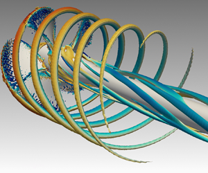
  $0.5\,\%$, respectively, when compared with experimental data. We made a qualitative comparison with results reported in high-resolution LES (Kumar & Mahesh Reference Kumar and Mahesh2017; Posa et al. Reference Posa, Broglia, Felli, Falchi and Balaras2019) where wall-resolving LES were performed, involving the use of a very large number of grid points. Some quantities such as axial velocity, vorticity magnitude, turbulent kinetic energy, root mean square and turbulent SGS viscosity were plotted at different sections perpendicular to the mean flow. The instability of the tip vortex occurred at approximately three diameters downstream, where larger levels of turbulent kinetic energy are observed. A population of large-scale vorticity was observed in the wake, although in the simulation the mutual induction and interaction between the tip vortex and that emitted at the hub was not observed, basically due to the fact that in pulling conditions the hub is replaced by the shaft. In this sense two main stable vortex structures develop, one being the tip vortex and the other the shaft vortex. This is shown in figure 2(a) where isosurfaces of the quantity
  $Q D^{2}/U_0^{2} = 80$ (
 $Q=0.5 (||\varOmega ||^{2}-||S||^{2}$) where
  $\varOmega$ and
  $S$ are the instantaneous rotation rate tensor and deformation rate tensor, respectively) are plotted coloured with the vorticity magnitude and the Lighthill term
  $\partial _{x_i x_j} T_{ij}$. The figure highlights the presence of the main vortical structures, the shaft vortex being persistent up to five diameters downstream. Figure 2(b) shows the same isosurfaces as (a), but coloured using the Lighthill term, which gives an indication of the regions of the wake where noise sources are more intense.

Figure 1. Computational grid adopted for the LES of the propeller in uniform flow.

Figure 2. Isosurface  $Q = 20\,000$ (non-dimensional
  $Q D^{2}/U_0^{2} = 80$, optimal value for the visualization of the two vortex structures): (a) contour of non-dimensional vorticity magnitude; (b) contour of Lighthill term.
The acoustic analysis related to this simulation had a clear outcome. Indeed, the authors observed a strong tonal noise at the rotational frequency, whose cause was recognized to be the strong vortex, that rolls up around the shaft. Being caused by a structure present in the wake, this acoustic signal was intercepted by the volume terms. Our results corroborated the findings of Ianniello (Reference Ianniello2016), who stated that ‘the usual assumption of believing the flow non-linear sources to be negligible for blades rotating at low subsonic speed is totally wrong when applied to hydroacoustics’. These results are in some sense quite new, since, in high-speed aeroacoustics, for a long time, it has been believed that the contribution to the noise coming from the wake is negligible compared with the linear terms. This is certainly true for helicopter blades, working in the compressible regime and characterized by very-high-pressure loads over the moving surfaces; however, as shown by other authors (see for example the comparison of measurements with numerical results reported in Ianniello, Muscari & Di Mascio Reference Ianniello, Muscari and Di Mascio2014) and also discussed in the present paper, this is not the rule in other physical configurations, like those studied herein and, in general, in low-Mach-number cases. Another example which is consistent with our results comes from the analysis of the database produced in the huge simulation of Posa et al. (Reference Posa, Broglia, Felli, Falchi and Balaras2019). The authors carried out a simulation of a seven-blade marine propeller, in an open-water pushing condition, adopting a grid of approximately 800 million cells. The acoustic computations carried out using the acoustic analogy revealed a strong broadband low-frequency noise, coming exclusively from the wake (Broglia et al. Reference Broglia, Cianferra, Posa, Felli and Armenio2020). In addition, the contribution of the wake to the far-field noise was shown to be more important than that coming from the linear part. The fact that the signal in Posa et al. (Reference Posa, Broglia, Felli, Falchi and Balaras2019) and Broglia et al. (Reference Broglia, Cianferra, Posa, Felli and Armenio2020) appears more broadband compared with the signal observed in the present work is mainly due to the different operating conditions and geometry of the propeller, namely, to the pulling low-loading condition reproduced in Cianferra et al. (Reference Cianferra, Petronio and Armenio2019b) versus the pushing high-loading conditions of Posa et al. (Reference Posa, Broglia, Felli, Falchi and Balaras2019). Indeed, the shaft located downstream the propeller, as it is in the case herein discussed, gives rise to a stable shaft vortex, identified as a main source of noise; in the work of Posa et al. (Reference Posa, Broglia, Felli, Falchi and Balaras2019) a hub vortex develops, it travels downstream and interacts with the tip vortex causing a broader spectrum.
2.2. The acoustic field
The diameter of the model-scale propeller is  $D_m = 0.25 \ \textrm {m}$ and the scaling factor adopted is
  $\lambda = 24$. The purpose is to use our data of pressure and velocity fields and to apply the FWH equation, first using imperfect similarity and successively using perfect similarity. Although the analysis has a general importance, here, we use hydrodynamic scaling. According to (2.4) and following the previous discussion, in the case of perfect similarity, we consider
  $c_{0_m}=c_{0_f}/\sqrt {\lambda }$, and in the case of imperfect similarity we consider
  $c_{0_m}=c_{0_f}$; here
  $c_{0_f} = c_{w} = 1400\ \textrm {m}\ \textrm {s}^{-1}$, where subscript
  $w$ denotes water. We calculate the dimensional acoustic pressure contributions associated with the single integrals of the FWH equation, for both procedures. We compute the acoustic pressure through (2.1) which corresponds to the original formulation proposed by Ffowcs-Williams and Hawkings. Over the years, a number of formulations have been developed depending on the problem under investigation. Specifically, efforts have been devoted to the computation of the noise generated by the wake, nowadays understood as to be responsible for the low-frequency part of the spectrum. Among others, the porous formulation (Di Francescantonio Reference Di Francescantonio1997) widely used in recent hydroacoustic noise applications allows us to neglect the volume terms. Recently this problem was carefully investigated by Cianferra et al. (Reference Cianferra, Ianniello and Armenio2019a). The authors found that the direct computation of the volume terms under the assumption
  $t=\tau$ (thus neglecting the time delays) is accurate in a large number of cases and also provided a criterion for the use of this computationally cheap and effective method. The authors also showed that the direct evaluation of the volume integral provides results more accurate than those obtained using the porous formulation, the latter being too sensitive to the position of the porous surface around the body and the wake. Details on the methodology are given in Cianferra et al. (Reference Cianferra, Ianniello and Armenio2019a) and are not duplicated here. For the evaluation of the volume terms we consider the fluid-dynamic instantaneous LES data contained within a cylindrical domain of volume
  $W$, diameter equal to
  $1.16D$ aligned with the propeller axis. For the evaluation of the linear terms we use the pressure over the propeller surface
  $S$ and its own velocity.
Six microphones are selected, whose positions are reported in table 1 and sketched in figure 3: two (1,2) are chosen on the propeller plane, at increasing distance from the propeller axis; two (3,4) are placed in the wake region at a distance of approximately  $14D$ from the centre of the propeller, over lines passing through the centre of the propeller and inclined by different angles with respect to the symmetry axis (respectively
  $45^{\circ }$ and
  $15^{\circ }$); two (5,6) are located in the far wake, over the propeller axis. Since the FWH terms decay differently with source–observer distance
  $r$, their own contribution varies considerably depending on the locations of the microphones. First, we analyse the time records over
  $t^{*}=4$ of full-scale acoustic pressure evaluated by means of the FWH equation, using the perfect scaling and the imperfect one, respectively. This is carried out both for the linear terms and for the nonlinear terms. Successively, we evaluate the spectra in decibel scale of the acoustic pressure obtained using the two procedures. In the following analysis we refer to full-scale quantities, indicating the FWH terms as
  $Th$,
$Th$,  $L1$,
$L1$,  $L2$,
$L2$,  $V1$,
$V1$,  $V2$ and
  $V3$.
$V3$.

Figure 3. Microphones considered for the acoustic analysis, listed in table 1 together with fluid-dynamic computational domain sketch (black box). Figure is not to scale.
Table 1. Microphones considered for the acoustic analysis;  $x$ is the streamwise direction with negative values indicating the downstream direction.

Figure 4 contains the time signals of the full-scale acoustic pressure associated with the linear terms, evaluated using the two methods. Note that, since the first and third terms of (2.10) scale perfectly, the time signals are the same in the two cases, whereas the time signal of the second term of (2.10) changes, increasing by  $\sqrt {\lambda }$. For the microphones
  $1 \text{ and }2$ (a,b) placed on the plane of the propeller, the thickness noise term prevails over the others, whereas the third term (
 $L2$) is always very small. The second term (
 $L1$), whose evaluation at the model scale using the speed of sound of water introduces errors, becomes increasingly important with the increase of the distance from the noise source since it decays with
  $1/r$. However, its own contribution remains substantially smaller than the thickness term. The situation is similar for the microphones
  $3 \text{ and }4$ placed in the wake zone (c,d), not very far from the propeller. In these cases, the error introduced by imperfect scaling is very small. The situation dramatically changes for the microphones
  $5 \text{ and }6$ placed in the far wake over the axis of the propeller (e, f) where, for symmetry reasons, the thickness term is zero. The error introduced by imperfect scaling, which affects the second integral, becomes increasingly large with increasing distance from the propeller. This can be attributed to the fact that
  $L1$ decays with
  $1/r$ whereas
  $L2$ decays with
  $1/r^{2}$.


The time records of the full-scale acoustic pressure associated with the FWH nonlinear volume terms are given in figure 5 for the six microphones. Note that, in this case, two out of three terms scale imperfectly, namely  $V1$, whose scaling properties were exploited in the seminal research of Lighthill, and
  $V2$ whose scaling properties are discussed in the present work. At the microphone
  $1$ which is close to the propeller (a), the term which scales perfectly (
 $V3$) is dominant. This is reasonable since the microphone is very close to the source and
  $V3$ contains
  $1/r^{3}$ in the integral kernel, while
  $V1$ and
  $V2$ contain respectively
  $1/r$ and
  $1/r^{2}$ in their integral kernels. Moving to microphone
  $2$ placed far from the source, the contribution of imperfect scaling becomes increasingly important as well as the error in the evaluation of the noise, as shown in figure 5(b). In the wake, out of the propeller disk, (microphones
  $3 \text{ and }4$) the three volume terms have comparable importance (c,d) and thus the imperfect scaling error is not negligible. In the far wake, over the propeller axis, due to the discussed different decay rate of the kernels of the volume integrals, the error associated with the imperfect scaling becomes increasingly important with increasing distance from the noise source. Some considerations derive from this analysis: first, comparing figures 4(f) and 5(f) it clearly appears that, downstream of the propeller, the nonlinear contribution given by the wake is an order of magnitude larger than that given by the linear terms; second, in the very near field the thickness term prevails over the unsteady loading term, due to the significant contribution given by the rotation of the solid elements, stating the need to consider a more complete form of the FWH equation even in the simplified linear analysis.


To highlight how imperfect scaling affects the total signal, in figure 6 we show the difference between the spectra, in terms of sound spectrum level (SPL) for the six microphones. Specifically, for each microphone we calculate the entire spectrum given by the sum of the six integral contributions, using the perfect scaling and the imperfect one. The decibel scale is obtained computing  $SPL = 20 \log _{10} fft(p(t))/p_{ref}$, with
  $fft(p(t))$ the Fourier transform of the time signal
  $p(t)$ expressed in Pascals and
  $p_{ref} = 1\ \mathrm {\mu } \textrm {Pa}$. The frequency is made non-dimensional with the revolution frequency
  $f_r = n \ \textrm {Hz}$,
  $n$ being the number of revolutions per second.

Figure 6. SPL of FWH signal: imperfect similarity (dashed red lines); perfect similarity (solid blue lines). The microphones are those listed in table 1.
The analysis of the spectra shows that, very close to the propeller (microphone 1, panel a), as expected, the two methods give practically the same result. This occurs because the dominant terms in the near field, namely  $Th$ and
  $V3$, scale perfectly. Further, we may observe that, close to the propeller, two main peaks dominate, one at the rotation frequency
  $f/f_r = 1$ and the other one at the blade frequency
  $f/f_r = N$ (
 $N$ is number of blades). It is worth noting also the appearance of sub-harmonics of the blade frequency, at
  $f/f_r = 2,3,4$. A specific analysis of the fluid-dynamic versus acoustic field (not shown) suggests that, at microphone 1, which is very close to the propeller, the signal is largely affected by the complex interaction between the various acoustic sources. We observed a rapid decay of the aforementioned sub-harmonics considering other microphones (not shown here) located on the propeller plane, at gradually increasing distances. At microphone
  $2$ a substantial difference of approximately 20 dB is observed, due exclusively to the difference previously observed in the analysis of nonlinear terms, figure 5(b). Thus, the imperfect scaling is not conservative with respect to the expected maximum noise level, since it underestimates the noise signal at the full scale. At microphones
  $3$ and
  $5$ the imperfect scalings of terms
  $L1$ and
  $V1$ are not able to produce significant variation in the spectrum, because they are less important than the terms scaling perfectly (namely
  $Th$ and
  $V3$) except for a slight drop of the perfect similarity signal, that may explained by a destructive interference between the term
  $V1$ and
  $V3$ occurring when
  $V1$ scale perfectly (figure 5c,e).
The fourth microphone is placed in the wake, with an angle of  $15^{\circ }$ with respect to the propeller axis. There, the contribution of
  $V3$ becomes comparable to that of the other two volume terms, therefore, the error introduced by imperfect scaling is noticeable over the whole spectrum, as shown in figure 6(d). At microphone
  $6$, located in the far wake, the signal obtained by the perfect scaling, resulting from the composition of solid lines (red, black and green) of figure 5( f), gives rise to a tonal signal at the rotation frequency. Actually, this is mostly given by the
  $V1$ term, since the
  $V2$ and
  $V3$ term signals are in opposition of phase and tend to cancel out. Similarly, the signal obtained with imperfect scaling, composed of the sum of solid green line and dotted red and black lines of figure 5( f), is tonal at the rotation frequency, given exclusively by the dominant term
  $V3$. Overall, the differences in the spectra are essentially due to the relative importance of the terms which scale imperfectly over those which scale perfectly.
To summarize, the analysis shows that carrying out laboratory-scale experiments using the speed of sound of water introduces a scale effect rendering incorrect the evaluation of the full-scale acoustic pressure starting from experimental data. The error is only partially associated with the noise propagating from the propeller surface (linear terms) and, more significantly, it is due to the imperfect scaling of the noise generated by the fluid-dynamic field in the wake around the propeller. The error is negligible close to the propeller, where the signal is dominated by terms  $Th$ and
  $V3$ which scale perfectly, and, in general, the peak at the rotation frequency is well reproduced even by imperfect scaling. However, far from the acoustic source, in the high-frequency range, considerable differences (up to about 20 dB) arise, between the signal obtained with the perfect scaling and that obtained with the imperfect scaling. Imperfect scaling introduces an underestimation of some noise source terms at the full scale, hence the imperfect scaling procedure is not conservative with respect to the noise level emitted by the full-scale propeller.
3. Acoustics in the presence of a free surface
In this section we discuss the effect of a reflecting surface on the noise generated by a source and propagated in the medium. Without losing generality, the surface is considered flat, meaning that for a marine propeller close to the free surface the flow field is that of a  $Fn = 0$ condition. In other words, in this case the presence of the free surface is negligible for the fluid-dynamic field, although it may be important for the acoustic one.
We first analyse the properties of simple acoustic fields (i.e. the monopole) close to a reflecting surface, and successively we study the case of a complex source which exhibits a non-trivial directivity and rotation around an axis (a marine propeller in the present investigation).
3.1. Monopole source near a free surface
Reflection is a crucial aspect of noise propagation in an underwater environment, and is quite a complex topic in the presence of interfaces and salinity/temperature variation in the fluid column (for a discussion see, among others, Athanassoulis et al. Reference Athanassoulis, Belibassakis, Mitsoudis, Kampanis and Dougalis2008, Reference Athanassoulis, Belibassakis, Gerostathis and Prospathopoulos2018). The problem of interfaces is shared by a number of marine engineering systems, among others, ship propellers, marine turbines and wind turbines mounted at sea. However, the presence of archetypal reflecting interfaces may be addressed easily by applying the method of images in case of time-domain wave equation (see for details Rienstra & Hirschberg Reference Rienstra and Hirschberg2004). The main difference with respect to the unbounded domain is that, in the presence of a free surface, two acoustic contributions arrive at the microphone: the direct signal coming from the source, and that reflected by the free surface. A free surface is a sharp interface which reflects the signal in the interior of the field and where  $p=0$; it is different from a solid surface which reflects in the interior and where the signal is doubled (see Rienstra & Hirschberg Reference Rienstra and Hirschberg2004). For this reason, in the presence of a free surface the reflection is mimicked by the image of the source, placed anti-symmetrically to the real source with respect to the plane of the free surface, thus having opposite sign with respect to the real source.
A monopole is a pressure field generated by a pulsating sphere. The pressure field has spherical symmetry and may be represented by harmonic waves of angular frequency  $\omega = 2{\rm \pi} f$, travelling outward from the source point
  $\boldsymbol {x}_s$
 \begin{equation} p(\boldsymbol{x},t) = \frac{p_I}{r} \sin(\omega t - k r), \end{equation}
where  $r = |\boldsymbol {x} - \boldsymbol {x}_s|$,
  $p_I$ is the intensity of the source expressed in
  $\textrm {Pa}\ \textrm {m}$ and the wavenumber
  $k = 2 {\rm \pi}/ c_0 T= \omega / c_0$. Note that, here, we consider the real part of the source, given by a sine wave. In the presence of a free surface we must consider the contribution of two monopoles, placed anti-symmetrically with respect to the free surface. One is placed at
  $\boldsymbol {x}_s = (x,y, z) = (0, 0, 0)$, with the reflection plane located at
  $y=L$. The imaginary source is located at
  $\boldsymbol {x}_i=(0, 2L, 0)$. With
  $r_1 = |\boldsymbol {x} - \boldsymbol {x}_s|$ and
  $r_2 = |\boldsymbol {x} - \boldsymbol {x}_i|$, at any point
  $\boldsymbol {x}$, the acoustic pressure is built of the sum of the two contributions
 \begin{equation} p(\boldsymbol{x},t) = \frac{ p_I}{r_1} \sin(\omega t - k r_1) - \frac{ p_I}{r_2} \sin(\omega t - k r_2). \end{equation}
 The imaginary monopole has negative sign, giving  $p=0$ at the surface.
Now, we make (3.2) non-dimensional by considering a signal amplitude  $p_0$, a time scale
  $T= 2 {\rm \pi}/\omega$ and a length scale
  $L$, the distance of the source from the free surface. Introducing the non-dimensional variables
  $p* = p/p_0$,
  $t^{*} = t \omega /2{\rm \pi}$,
  $r_i^{*} = r_i/L$, with
  $i=1,2$, and considering that
  $sin \theta = - \sin (\theta + {\rm \pi})$ we obtain
 \begin{equation} p^{*} = \frac{p^{*}_I}{r^{*}_1} \sin\left(2{\rm \pi} t^{*} - \frac{\omega L}{c_0} r_1^{*}\right) + \frac{ p^{*}_I}{ r_2^{*}} \sin\left(2{\rm \pi} t^{*} - \frac{\omega L}{c_0} r_1^{*} - \frac{\omega L}{c_0} (r_2^{*}-r_1^{*}) + {\rm \pi}\right), \end{equation}
with  $p^{*}_I=p_I / p_0 L$. The non-dimensional intensity of the monopole depends on a pressure impulse and the distance from the free surface. Here, we explicitly highlight the phase lag between the two signals. Now, we exploit some properties of this monopole. We observe that the composition of the two signals (direct and reflected) is constructive or destructive depending on the phase lag between the signals. The second sine wave of (3.3) interferes destructively with the first one when
  ${\omega L}/{c_0} (r_2^{*}-r_1^{*}) \in [2m{\rm \pi} - {\rm \pi}/3, 2m{\rm \pi} + {\rm \pi}/3]$, with
  $m=0,\pm 1, \pm 2,\ldots$ integer numbers.
At any point of the free surface (where  $r^{*}_1=r^{*}_2$) the phase lag between the two sine waves is
  ${\rm \pi}$ and the signals cancel out. Close to the source location
  $r^{*}_1 \rightarrow 0$ and
  $r^{*}_2 \rightarrow 2$; the phase lag is given by
  $-2\omega L/c_0+{\rm \pi}$, so it tends to
  ${\rm \pi}$ (destructive interaction) for low frequencies and small
  $L$; however, for very small
  $r^{*}_1$, the contribution of the image monopole is negligible compared with that of the real source. At points located over the line passing through the two point sources and orthogonal to the free surface,
  $r^{*}_2=\pm r^{*}_1 + 2$ with positive sign for points located by the opposite side with respect to the free surface and negative sign for points located between the source and the free surface, with
  $r^{*}_1 < 1$. In the former case
  $r^{*}_2=r^{*}_1 + 2$ and the phase lag between the two signals is
  $-2 \omega L /c_0+{\rm \pi}$. This value gives destructive interaction when
  $(2m-1/3) {\rm \pi}< 2 \omega L/c_0 < (2m+1/3) {\rm \pi}$, meaning that, for a given distance
  $L$ from the free surface, there is a range frequencies such that the free surface causes a destructive interaction of the signals, although the total signal cannot be zero because the contribution of the real signal, as in the previous case
  $r^{*}_1 \rightarrow 0$, is always larger than that of the image one in the near field. In the far field, when
  $2/r^{*}_1 \sim 0$,
  $r^{*}_2/r^{*}_1 \sim 1$, the magnitude of the two signals is comparable and the phase lag behaves as discussed above. For points by the side of the free surface
  $r^{*}_2=-r^{*}_1 + 2$, with
  $r^{*}_1 < 1$, the two sine waves of (3.3) are in phase when
  $(1-r^{*}_1) = {\rm \pi}c_0/2 \omega L < 1$ and fully destructive for
  $r^{*}_1=1$, at the free surface as already discussed. However, also in this case, for
  $r^{*}_1 \longrightarrow 0$ the intensity of the real signal tends to be larger than that coming from the image source. Considering the points over a line passing through the real source and parallel to the free surface, we are in the case where
  $r^{*^{2}}_2 = 2^{2} + r^{*^{2}}_1$. Note that the microphones located on the propeller wake fall into this category. Dividing by
  $r^{*}_1$, we obtain
  $r^{*^{2}}_2/r^{*^{2}}_1 = 1 + (2/r^{*}_1)^{2}$, which highlights that for
  $r^{*}_1 < 2$ the contribution of image source becomes small when compared with real source contribution, and for moderate-to-large values
  $r^{*}_1 > 2$,
  $r^{*}_2/r^{*}_1 \sim 1$ the two sources have comparable magnitude. For the phase, it is easy to show that destructive interaction requires
  ${\rm \pi} (2m-1/3)<4 \omega L/ [c_0 (r^{*}_2+r^{*}_1) ] <{\rm \pi} (2m+1/3)$. Finally, in the general cases, the two signals are in phase when
  $\omega L /c_0 (r^{*}_2 - r^{*}_1) = (2m+1){\rm \pi}$. The condition
  $r^{*}_1 \sim r^{*}_2$, which ensures a comparable amplitude of the two sine waves, leads to
  $\omega L/c_0 \gg 1$. Thus, pure doubling of the signal may occur at high frequencies or for large values of
  $L$.
$L$.
The discussion holds for a monopole field, or, in general for signals with spherical symmetry (for example airguns); however, when considering sources characterized by strong directivity, the analysis becomes more complex. For example, in figure 7 we show how the directivity of three types of elementary sources, monopole, dipole and quadrupole, changes in the presence of a free surface. We consider the real source located at a distance  $L$ from the surface, and the image source placed anti-symmetrically with respect to the surface. The microphones are located at distance
  $D_c$ from the real source. The monopole was already discussed above. In the cases of the dipole and quadrupole sources, the discussion for the monopole still holds mainly for angle of
  $270^{\circ }$, where the observer is on the line passing through the two sources. Also, changes in the shape of the directivity are observed under variation of the frequency
  $\omega$ and of the ratio
  $L/D_c$. This is the case, among others, of rotors, such as wind turbines or the ship propeller discussed in the previous section, which exhibit a dipole-like field and a quadrupole-like one for the linear and nonlinear parts of the noise signal, respectively. The rotation of the source adds complications, since the image rotates counterclockwise when the real source rotates clockwise. Specifically, in the presence of rotation the phase lag
  $\phi$ (consider a sinusoidal wave
  $\sin (\omega (t-\phi ))$ as an example) between the signals has an additional shift when compared with the case in the absence of rotation.

Figure 7. Directivity of (a) monopole, (b) dipole and (c) quadrupole. Unbounded domain (crosses); free surface (circles).
In the next section the method of images is applied to the marine propeller case and results analysed also in view of the discussion of the present section.
3.2. Rotating complex source near a free surface
Integral solution of a time-domain, non-homogeneous, wave equation in a homogeneous medium, makes use of the Green's function adopted under the assumption of free-space propagation. As for the monopole, the free surface is modelled by considering an additional imaginary source, which works as the real source mirror image with respect to the reflecting plane. As a result, certain boundary conditions are satisfied automatically by the presence of the mirror image. Instead of free-space Green's function, the half-space Green's function is adopted, which is built in such a way to consider both sources, real and imaginary.
The half-space Green's function is therefore the fundamental solution of the problem
 \begin{equation} \begin{cases} \displaystyle(\partial_{tt} - c^{2} \nabla^{2}) \boldsymbol{G}(\boldsymbol{x},t,\boldsymbol{x}_0,\tau) = \delta (\boldsymbol{x} - \boldsymbol{x}_0, t - \tau) & \boldsymbol{x} \in \mathbb{R}^{+},\\ \displaystyle \boldsymbol{G}(\boldsymbol{x}, t,\boldsymbol{x}_0,\tau) = 0 & \boldsymbol{x} \in \partial \mathbb{R}^{+}, \end{cases} \end{equation}
where the source  $\delta (\boldsymbol {x} - \boldsymbol {x}_0, t - \tau )$ is an impulse originating at time
  $\tau$, at point
  $\boldsymbol {x}_0$. Note that the boundary
  $\partial \mathbb {R}^{+}$ of the domain corresponds to the plane
  $\boldsymbol {x}=0$ and the homogeneous Dirichlet condition is placed to mimic the
  $p=0$ condition. The Green's function solving (3.4) for the three-dimensional space, has the form
 \begin{equation} \boldsymbol{G}(\boldsymbol{x},t,\boldsymbol{x}_0,\tau) = \frac{ \delta ( t - \tau - |\boldsymbol{x} - \boldsymbol{x}_0| )}{ 4{\rm \pi} |\boldsymbol{x} - \boldsymbol{x}_0| } - \frac{ \delta( t - \tau - |\boldsymbol{x} - \boldsymbol{x}^{*}_0| )}{ 4{\rm \pi} |\boldsymbol{x} - \boldsymbol{x}^{*}_0|}, \end{equation}
with  $\boldsymbol {x}^{*}_0$ being the image source location. Note that the first term, which corresponds to the real source impulse, is non-zero when
  $t = \tau + |\boldsymbol {x} - \boldsymbol {x}_0|/c_0$, while the impulse coming from the imaginary source arrives at the same point when
  $t = \tau + |\boldsymbol {x} - \boldsymbol {x}^{*}_0|/c_0$. This time delay gives a phase lag which may amplify or destruct the original signal, as already discussed for the archetypal sinusoidal wave of the monopole case.
The convolution of the half-space Green's function with the source term of the differential FWH wave equation leads to the integral equation describing the case of acoustic propagation in presence of the free surface  $\boldsymbol {x} = 0$.
We apply the method of images to the case of the marine propeller discussed in the previous section. Note that, given the peculiarities of the Green's function method, the free surface is approximated as a perfectly smooth plane, not disturbed by the presence of the propeller ( $Fn =0$). This does not limit the importance of the present study for a number of reasons: for the specific case of a marine propeller, laboratory tests are usually carried out in the
  $Fn \longrightarrow 0$ limit; in the general case of a complex source close to an interface (a wind or a marine turbine among others) the case of a flat surface in the most general one. The introduction of a wave system would introduce, at least, two more free parameters. To account for a non-flat free surface, methods different from the Green's function have to be used. This is beyond the scope of the present paper.
As in the previous section, the model-scale propeller has a diameter of  $D=0.25\ \textrm {m}$, it is centred at the origin of the frame of reference
  $\boldsymbol {O} = (0, 0, 0)$ and the wake develops along the negative
  $x$-axis. The speed of sound for the model-scale propeller is set to
  $c_0 = c_w /\sqrt {\lambda }$, with
  $\lambda = 24$, thus considering perfect similarity. Note that, in the present problem,
 \begin{equation} p^{*}=f(J,V_r,L/D), \end{equation}
with  $L/D$ the additional non-dimensional parameter, associated with the presence of the interface, controlling the problem; also, geometric similarity ensures that points behave similarly at the two scales when the ratio
  $L/D_c$ is the same, where
  $D_c$ is the distance of the microphone from the source. We first analyse the directivity, obtained considering 100 microphones placed on the
  $y=0$ plane (a vertical longitudinal plane), at constant distance
  $D_{c}$ from the source. In the plots, the distance from the centre indicates the value of the root mean square
  $p_{rms}$ of the acoustic pressure (in Pascals) at the microphone located at the corresponding angle. The analysis is performed for each single term of the FWH equation. The directivity is reported in figures 8 to 11 for an unbounded domain in the presence of the free surface. The directivity is calculated for two distances from the source, respectively
  $D_c = 10D$ in figures 8 and 10,
  $D_c = 100D$ in figures 9 and 11. Finally, we consider two values for the distance
  $L$ of the source from the free surface,
  $L = 2D$ in figures 8 and 9,
  $L = 8D$ in figures 10 and 11. In all plots, the downstream direction (the wake) is
  $180^{\circ }$; further, when considering the presence of the free surface, depending on
  $D_c$ and
  $L$ the range of angles at which we can observe the underwater acoustics (and therefore the directivity) changes; for this reason the values are not shown for angles giving microphones outside of the fluid domain.

Figure 8. Directivity of linear terms (a,c,e) and nonlinear terms (b,d, f), evaluated at a radius of  $10D$, on the plane
  $y=0$. Unbounded domain (blue crosses); free surface (red circle). Free surface at
  $L=2D$.

Figure 9. Directivity of linear terms (a,c,e) and nonlinear terms (b,d, f), evaluated at a radius of  $100D$, on the plane
  $y=0$. Unbounded domain (blue crosses); free surface (red circle). Free surface at
  $L=2D$.

Figure 10. Directivity of linear terms (a,c,e) and nonlinear terms (b,d, f), evaluated at a radius of  $10D$, on the plane
  $y=0$. Unbounded domain (blue crosses); free surface (red circle). Free surface at
  $L=8D$.

Figure 11. Directivity of linear terms (a,c,e) and nonlinear terms (b,d, f), evaluated at a radius of  $100D$, on the plane
  $y=0$. Unbounded domain (blue crosses); free surface (red circle). Free surface at
  $L=8D$.
As a preliminary test, we checked the cancellation of the acoustic pressure at the free surface, as required by the Dirichlet condition at the boundary. In all cases examined the model gives the expected result. We first observe that, for linear terms (left panels in figures 8 to 11), the intensity of acoustic pressure fluctuations is in general weaker than that produced by the nonlinear terms (right panels in the same figures), showing, once more, the importance of the latter with respect to the former. Note that, when considering the decibel scale with a reference pressure of  $1\ \mathrm {\mu } \textrm {Pa}$, the signals below
  $10^{-6}\ \textrm {Pa}$ correspond to negative values. The directivity of linear terms (dipole-like) remains nearly unchanged in all cases, when the presence of the free surface is considered. In particular, the terms are very small on the propeller axis in all cases, whether or not there is a free surface. The exception is the thickness term, which by symmetry reasons is zero in an unbounded domain and has non-zero values at
  $0^{\circ }$ and
  $180^{\circ }$ in the free-surface case. A signal amplification is observed in almost all cases. A verification of this result was carried out by analysing the time history of pressure signals (not reported here). In fact, at distances
  $D_c=10D$ or
  $100D$, the linear term signals are characterized by a wide spectrum, maintaining the rotation frequency
  $f_r = 15\ \textrm {Hz}$ as the dominant one. The signal coming from the imaginary source is comparable in amplitude and frequency content to the signal emitted by the real source, however, the discussion on the interaction properties of the monopole per se cannot explain this signal composition. As observed before, rotation may affect the composition of the signals. The phase lag occurring in the case of reflection and rotation is given by
  $\phi = L(r^{*}_2 - r^{*}_1)/c_0 + 1/f_r *1/2$, which, in our case, makes the low-frequency signal constructive. In particular, in the case
  $L/D_c = 0.02$, the interaction between the signals appears constructive up to
  $f \sim 20\ \textrm {Hz}$. In other words, the low-frequency amplification of the signal is the result of a combination of the phase lag discussed before for the monopole case and the effect of rotation. On the other hand, in the case
  $D_c=10D$ and
  $L=8D$ (
 $L/D_c\sim 1$), the intensity of the real source is much more relevant than the imaginary one, whose contribution is therefore negligible (figure 10).
The directivity of nonlinear terms exhibits a dipole-like shape for small distances from the source and tends to a quadrupole shape with large distances (see figures 9(b,d, f) and 11(b,d, f), respectively). In addition, the relative contribution of the nonlinear terms  $V1$,
$V1$,  $V2$ and
  $V3$ appears reversed in the transition from
  $D_c= 10D$ to
  $D_c=100D$. This is expected, given the law which rules the decay with distance from the source of the different terms; this justifies the prevalence of the third term when close to the source, case
  $D_c=10D$ in figure 8, and the increasing importance of the first and second terms at large distances (figure 9). For the cases
  $L/D_c=0.02$ and
  $L/D_c=0.08$, reported in figures 9 and 11, respectively, the quadrupole shape appears rotated by
  $90^{\circ }$ (red circles), so that the interaction of the signals is destructive by the free-surface side, on the propeller axis as well as on the propeller plane. Finally, as observed for linear terms, in the case
  $L/D_c=0.8$, the presence of the free surface is of minor importance. The results presented in this section show that the presence of the free surface substantially modifies the signal, giving a larger and larger contribution when
  $L/D_c \ll 1$.
4. Small- versus full-scale analysis in the presence of a free surface
In § 2 we have shown that some terms of the FWH equation scale imperfectly once the speed of sound at the laboratory scale is not rescaled according to the velocity ratio  $V_r$. This introduces errors when obtaining the full-scale acoustic pressure starting from small-scale values. Among the six integral terms of the FWH equation, the terms which can make a difference, when considering perfect or imperfect scaling, are the loading term
  $L1$ and the nonlinear terms
  $V1$ and
  $V2$. In § 3.2 we have observed that the presence of a free surface may change substantially the magnitude of some terms of the FWH equation, depending on the position and the distance of the microphone from the noise source
  $D_c$ and on the distance of the noise source from the free surface
  $L$, namely depending on
  $L/D_c$. Here, the scaling procedure discussed in § 2 is combined with the method of images, and applied to study the acoustic field generated by the marine propeller. The aim of this analysis is to quantify the error associated with carrying out laboratory-scale tests using the speed of sound of water in a (either physical or numerical) set-up without the free surface, and recalculating the full-scale acoustic pressure for a device working close to a free surface. The analysis is not necessarily concerned only with physical experiments, but also with numerical experiments carried out at the laboratory scale as discussed above. In addition, the presence of additional reflecting surfaces (like those present in a water tunnel) is here not considered. Considering that the errors associated with imperfect scaling for
  $L1$,
$L1$,  $V1$ and
  $V2$ are proportional to
  $\lambda ^{n}$,
  $\lambda ^{2n}$ and
  $\lambda ^{n}$, respectively (
 $n=1/2$ for hydrodynamic scaling), among the cases discussed in § 3.2, the plots of directivity show that the maximum error, when considering imperfect scaling in an unbounded domain, may occur when
  $D_c=100D$ and
  $L=2D$, thus
  $L/D_c = 0.02$. Conversely, the case with the minimum error is
  $D_c=10D$ and
  $L=8D$, thus
  $L/D_c = 0.8$. For each case, we consider three microphones located at three significant angles,
  $180^{\circ }$ (in the wake),
  $225^{\circ }$ (below the propeller over the diagonal) and
  $270^{\circ }$ (below the propeller), respectively.
For the two microphones on the propeller wake (figure 12a,b), the first linear term ( $Th$, blue lines) exhibits a significant variation; indeed, as already discussed, in unbounded domains the thickness term is negligible for reasons of symmetry on the propeller axis. The presence of the free surface significantly affects the directivity of the signal and a peak is observed at the rotation frequency, with a value of approximately
  $50\ \textrm {dB}$ (a).

Figure 12. Linear terms of FWH equation:  $Th$, blue lines;
  $L1$, red lines;
  $L2$, green lines. Perfect scaling with free surface, dashed lines; imperfect scaling with unbounded domain, solid lines.
Among the three linear terms, the one that scales imperfectly is the second one ( $L1$); we observe a difference of approximately
  $14\ \textrm {dB}$ (note that
  $20\log _{10}\sqrt (24) \sim 14$) between the two cases. This is very clear for
  $L/D_c = 0.8$, where the effect of the free surface is negligible. The constructive interference, observed in the study of directivity, is in fact more visible in the case
  $L/D_c = 0.02$ (d, f) where the signal accounting for the presence of the surface is amplified with respect of the single-source signal, of about
  $20\ \textrm {dB}$. At angle
  $180^{\circ }$ (figure 12a,b), mostly for the case
  $L/D_c = 0.02$, for
  $P^{L1}$ the peaks corresponding to the super harmonics of the rotation frequency are smoothed out due to destructive interaction with the image source signal. The simple analytical considerations of the previous section suggest that at
  $180^{\circ }$ the phase lag between the signals becomes
  $\phi = 4L/(r^{*}_2 + r^{*}_1)c_0 + 1/f_r *1/10$, which, with
  $r^{*}_2 \sim r^{*}_1 = 50$, is very small, and the signal of the image source is destructive over the whole high-frequency range.
In figure 13 we show the spectra of the nonlinear terms. The third term ( $V3$) scales perfectly; as a consequence, the signals for unbounded and bounded domains overlap in the case
  $L/D_c=0.8$ (a,c,e) when the effect of the free surface is irrelevant. On the other hand, destructive interference appears in case
  $L/D_c = 0.02$ (b,d, f) at angles
  $180^{\circ }$ and
  $270^{\circ }$, as previously observed in the directivity analysis.

Figure 13. Nonlinear terms of FWH equation:  $V1$, blue lines;
  $V2$, red lines;
  $V3$, green lines. Perfect scaling with free surface, dashed lines; imperfect scaling with unbounded domain, solid lines.
For the two other terms, we recall that multiplication of a pressure signal by  $\lambda = 24$ (needed for
  $V1$) and
  $\sqrt {\lambda }$ (needed for
  $V2$) gives an increase of approximately 27 and 14 decibels, respectively. Indeed, in the case
  $L/D_c=0.8$ (a,c,e) the signals increase by the factors
  $27$ and
  $14$ over the whole frequency range, due basically to imperfect scaling, since in this case the free surface does not affect the pressure signal. Conversely, in the case
  $L/D_c=0.02$ (a,c,e), the presence of the free surface reduces the gap between the signals at angles
  $180^{\circ }$ and
  $270^{\circ }$, due to the substantial destructive interaction between the direct and reflected acoustic waves. This is not true for the signal at angle
  $225^{\circ }$, depicted in figure 13(d), where both scaling procedure and free-surface constructive interaction make the signal amplified with respect to the case of imperfect scaling in an unbounded domain.
Finally, the total signals are reported in figure 14, in the case of perfect scaling with a free surface and in the case of imperfect scaling in an unbounded domain. In all cases, the dominant contribution to the complete FWH signal comes from nonlinear terms, so we can refer to the previous figure 13 to explain the behaviour of the total acoustic signal. The difference between the signals in figure 14(a,c,e) is mainly the result of the sum of  $V1$ and
  $V3$. Indeed,
  $V3$ dominates close to the source (
 $D_c = 10D$) and scales alike in both the scaling procedures. Further,
  $V1$ when correctly scaled, makes the signal increase mostly in the range of high frequencies. On the other hand, the differences appear very small in most of the frequency range and, in particular, in the region where the signal peaks. Far from the source (
 $D_c = 100D$) (b,d, f) the most relevant contribution comes from
  $V2$. The difference given by the perfect scaling of the second term (
 $+14\ \textrm {dB}$) is reduced, as observed in the previous figure 13 at angles
  $180^{\circ }$ and
  $270^{\circ }$ and enhanced at
  $270^{\circ }$, due to the presence of the free surface.

Figure 14. Complete signal given by the FWH equation. Perfect scaling with free surface, dashed black line; imperfect scaling with unbounded domain, solid blue line.
5. Discussion and concluding remarks
In the present paper we have analysed the scaling properties of all integral terms of the FWH equation, in conjunction with perfect/imperfect scaling when data obtained at laboratory scale are used for prediction at the full scale.
Since Lighthill's seminal work, scaling properties of monopole, dipole and quadrupole sources have been exploited, finding dependence with the Mach number, no matter what the fluid-dynamic regime is. Such scaling laws apply to the FWH terms decaying as  $1/r$. We have corroborated and extended the classical theory, evaluating scaling of the additional terms (linear and nonlinear) decaying as
  $1/r^{2}$ and as
  $1/r^{3}$, commonly overlooked in many applications. In order to quantify the error associated with the imperfect scaling we have considered the case of a benchmark marine propeller, operating in open-sea, uniform-flow conditions, for a single-phase medium.
The study has also been motivated by the discussion contained in the fundamental paper (Brentner & Farassat Reference Brentner and Farassat2003) where the authors stated in the conclusions that ‘... more understanding of the rotor wake and tip vortices is needed’. In spite of that, most recent research has primarily considered two main mechanisms of noise production, namely the unsteady pressure load over the solid surface and the thickness term, responsible of the broadband spectrum in the range of high frequencies; this led us to consider the linear terms of the FWH equation as the dominant ones and the only ones worthy of consideration.
In recent years, with the increasing application of acoustic analogies to underwater noise problems, this issue has been progressively revisited. Several works (among others Ianniello et al. Reference Ianniello, Muscari and Di Mascio2013; Ianniello Reference Ianniello2016) have proved and highlighted the need to accurately evaluate the nonlinear terms. Not surprisingly, most of the works on propeller noise adopt the FWH porous formulation, which involves the calculation of the quadrupole terms, or more recently the direct evaluation of the volume terms as discussed by Cianferra et al. (Reference Cianferra, Ianniello and Armenio2019a).
As shown in the present paper, the wake plays an important role in the composition of the noise spectrum. The more it contains coherent structures and/or is characterized by a well-defined periodicity, the more its noise signature is characterized by pronounced peaks at particular frequencies. Moving from a disorganized wake to a coherent-structure-containing wake corresponds to the transition from white-noise type to tonal-noise type. Moreover, the latter may persist over long distances, especially if it is a low-frequency tonal noise and if it propagates in a waveguide-shaped environment (such as the ocean). As an example, figure 13 in the recent paper of Cianferra, Armenio & Ianniello (Reference Cianferra, Armenio and Ianniello2018) shows a comparison of the noise associated with the wake of a cube and that associated with the wake of a square-section cylinder. The figure highlights that: (i) an elongated (nearly two-dimensional) object gives rise to a wake louder than that developed downstream of a bluff body; (ii) the wake of the elongated object is louder than the noise emitted by the impact of the fluid over the body (loading noise).
Looking at the recent literature, it clearly appears that the relevance of nonlinear terms goes beyond the nature of the fluid (whether air or water). As an example, the recent experimental study on the noise produced by the Sevik rotor in air, in the incompressible-flow regime, ingesting turbulence generated by a boundary layer (Alexander et al. Reference Alexander, Devenport and Glegg2017), shows a broadband spectrum where a substantial contribution to the low frequencies is present after subtraction of the background noise (see their figure 4b), suggesting the possible importance of quadrupole noise associated with the volumetric turbulence contribution. Our analysis shows that, apart from the  $Ma$ and
  $Ma^{2}$ scaling of the terms
  $L1$ and
  $V1$, respectively, already discussed in the literature, the terms
  $Th$,
$Th$,  $L2$ and
  $V3$ are Mach independent and the term
  $V2 \sim Ma$. This may have important consequences regarding whether or not Mach similarity is satisfied when laboratory-scale data have to be used at the full scale.
We have calculated the error associated with the scaling discussed above when using laboratory-scale data for full-scale prediction under the assumption that the speed of sound is nearly unchanged at the two scales. In particular, the scaling is expressed in terms of a geometrical scale factor  $\lambda$ using the fact that
  $U_f=\lambda ^{n} U_m$ with
  $\lambda > 1$ and
  $n$ depending on the problem investigated. In particular,
  $Ma$-independent terms scale perfectly, namely the thickness term, the loading term (
 $L2$) and the nonlinear volume term proportional to
  $T_{ij}$ (
 $V3$); for the other terms, the error is
  $\lambda ^{n}$ for the unsteady loading term (
 $L1$) and for the nonlinear term proportional to
  $\partial T_{ij} / \partial t$, whereas the error increases to
  $\lambda ^{2n}$ for the remaining (
 $V1$) nonlinear term proportional to
  $\partial ^{2} T_{ij}/\partial t^{2}$, namely that decaying as
  $1/r$ and already analysed in the fundamental work of Lighthill. When applying the Froude similarity to scale the velocity field, this implies
  $n=1/2$ and the errors go consequently.
It may be worth noticing that, when dealing with hydrodynamic noise sources, mostly in the very low Mach regime (hence treated as incompressible flows), the similarity with respect to the Mach number is clearly not considered. Neither when performing fluid-dynamic simulation, nor (to the best of the authors' knowledge) when scaling the acoustic results. In the present work we have stressed this point, highlighting how the acoustic spectrum may change (or not) if the Mach similarity is addressed in the scaling procedure of the acoustic results.
To summarize, the results of the present study are of general use and are concerned with both physical and numerical laboratory-scale experiments, although in the present study we consider the case of a numerical simulation of an isolated ship propeller.
The reference data were obtained in a previous investigation and are relative to a small-scale propeller, in a pulling condition, studied numerically using LES and considering an unbounded domain. It clearly appears that small-scale experiments, aimed at the evaluation of the noise generated by a device immersed in a fluid, should be carried out at Mach similarity, consequently scaling properly the speed of sound. For the case under investigation that uses hydrodynamic scaling, the speed of sound needs to be scaled by  $\sqrt {\lambda }$, otherwise the acoustic field is evaluated incorrectly, meaning that it may be not representative of that emitted by the full-scale device. When performing numerical experiments, setting an idealized fluid whose properties fit those required by perfect similarity is not difficult, this is not the case of physical experiments, where it is not straightforward using fluids having a speed of sound much smaller than that of water.
This part of the research shows that the near field is nearly unaffected by imperfect scaling because there the thickness term, which is  $Ma$-independent, dominates. The intermediate-to-far field noise is dominated by the nonlinear terms, two out of three of which scale imperfectly; as a consequence imperfect scaling affects the full-scale signal.
As a second aspect, the present research was aimed at understanding and quantification of the effect of a free surface not in a Froude number sense, but as a surface reflecting the acoustic waves in the medium. The overall acoustic field results from a composition of two signals, the one directly arriving from the acoustic source and the one reflected by the free surface. The combination of the signals may be either destructive or constructive. We have taken advantage of simple archetypal acoustic sources, to explain the composition of the signal in terms of amplitude and range of frequencies. This simplified theory, once the rotation rate of the device is taken into account, may give information about the range of frequencies where the signals combine destructively or constructively, supplying, in the latter case, an amplification of the noise produced by the propeller placed near the free surface.
Finally, we have evaluated the overall error associated with the combination of effects, considering a virtual experiment carried out using imperfect similarity in an unbounded domain and another one which uses perfect similarity and considers the presence of the free surface. The results show that the noise spectrum may be substantially modified, with a general underestimation of the noise propagated in the far field, for small values of  $L/D_c$, and for particular directions only. Indeed, the directivity of nonlinear terms, which are found to be dominant at large distances, shows that, only in a limited range of angles is the signal affected by the presence of a free surface amplified with respect to the unbounded case. In all other directions, the decrease of the signal due to the interaction with the free surface is such to reduce the error caused by the imperfect scaling. On the other hand, the general error appears very small in the near field (
 $L/D_c \sim 1$) in the most significant part of the frequency spectrum, making the results of small-scale experiments carried out using imperfect scaling in the absence of a free surface still significant for the evaluation of the full-scale noise in the near field.
We point out that in the present study the Reynolds number similarity was not considered. Under  $J$ and Froude similarity, typically
  $Re_f \sim 10^{2} Re_m$. This may produce some differences in particular in the wake although, for rotors, recent literature has proved that beyond a certain Reynolds number the turbulent wake is inertia dominated and exhibits self-similarity. However, this issue may deserve additional study.
Finally, the results of this study may be useful: (i) for the improvement/development of simplified regression/based approaches to be used during the early design stages; (ii) in view of processing laboratory-scale data to obtain full-scale values at the same time removing the problem of imperfect scaling, thus opening new and so far unexplored analysis scenarios. In particular, when the fluid-dynamic field is incompressible, laboratory-scale velocity and pressure data available over certain surfaces (using, for example PIV or other cutting-edge experimental techniques) can be first scaled at the full scale and successively post-processed using the FWH equation, as done in the field of computational acoustics using direct numerical simulation or LES data. This procedure may be considered conformed to the scaling suggested in this work and can be a subject of future research.
Declaration of interests
The authors report no conflict of interest.


