


1. Introduction
Planetary and stellar magnetic fields are ubiquitous throughout the observable Universe. These magnetic fields are thought to be actively generated by the convection-driven motion of electrically conducting fluid (Ossendrijver Reference Ossendrijver2003; Jones Reference Jones2011). Rayleigh–Bénard convection (RBC), consisting of a fluid layer contained between plane parallel boundaries, is a common system in which to study convection due to its simplicity, whilst retaining the primary physical features expected to be important in many natural systems (Meneguzzi & Pouquet Reference Meneguzzi and Pouquet1989; Cattaneo Reference Cattaneo1999). Although RBC has been investigated in great detail with regard to electrically insulating fluids, the influence of dynamo action on heat and momentum transport is less well understood. This study reports on numerical results of a broad parameter survey of RBC-driven dynamos.
Natural dynamos can be distinguished by the characteristic length scale of the self-generated magnetic field, relative to that of the forcing length scale. Large-scale dynamos generate magnetic fields that are both system scale and forcing scale, whereas small-scale dynamos generate magnetic fields with typical length scales that are comparable with, or less than, the typical velocity length scale (Meneguzzi, Frisch & Pouquet Reference Meneguzzi, Frisch and Pouquet1981; Rincon Reference Rincon2019; Tobias Reference Tobias2019). Breaking the reflectional symmetry of the flow field via the Coriolis force, for instance, is known to be conducive to large-scale dynamo action (Parker Reference Parker1955; Steenbeck, Krause & Rädler Reference Steenbeck, Krause and Rädler1966; Moffatt Reference Moffatt1970; Childress & Soward Reference Childress and Soward1972; Calkins et al. Reference Calkins, Julien, Tobias and Aurnou2015); such effects are likely to be important for the generation of the global-scale components of planetary and stellar magnetic fields. However, small-scale dynamos are also relevant, especially with regard to the Sun's outer convective layer, where an intense small-scale field is generated.
Two global diagnostic quantities of central interest in convection are the rate of heat transport through the layer and the typical flow speed, as measured by the non-dimensional Nusselt number,  $Nu$, and the Reynolds number,
  $Re$, respectively. For a fixed value of the thermal Prandtl number,
  $Pr = \nu /\kappa$ (where
  $\nu$ is the kinematic viscosity and
  $\kappa$ is the thermal diffusivity), convective flow regimes depend on the non-dimensional Rayleigh number,
  $Ra$; functional relationships of the form
  $Nu = f(Ra)$ and
  $Re = g(Ra)$ (where
  $f$ and
  $g$ denote generic functions) are sought. For heat transport with
  $Pr=O(1)$ in non-rotating systems, theory has suggested both a
  $Nu \sim Ra^{1/3}$ scaling, from marginal stability analysis of the thermal boundary layer (Malkus Reference Malkus1954), and a
  $Nu \sim (Ra/Pr)^{1/2}$ scaling, which assumes an ultimate regime in which the entire fluid layer becomes turbulent (Kraichnan Reference Kraichnan1962; Spiegel Reference Spiegel1965); the former is independent of the fluid layer depth, whereas the latter is independent of diffusion coefficients (
 $\nu , \kappa$). The convective ‘free-fall’ scaling of
  $Re \sim (Ra/Pr)^{1/2}$, thought to arise from a balance between nonlinear advection and the buoyancy force, and expected to be valid when
  $Re \gg 1$, is consistent with the
  $Nu \sim (Ra/Pr)^{1/2}$ heat transport scaling (e.g. Ahlers, Grossmann & Lohse Reference Ahlers, Grossmann and Lohse2009). Laboratory experiments and numerical simulations observe a
  $Nu \sim Ra^{2/7}$ scaling over a significant range in
  $Ra$ (e.g. Castaing et al. Reference Castaing, Gunaratne, Heslot, Kadanoff, Libchaber, Thomae, Wu, Zaleski and Zanetti1989; Shraiman & Siggia Reference Shraiman and Siggia1990; Cioni, Ciliberto & Sommeria Reference Cioni, Ciliberto and Sommeria1997), and a transition to a
  $Nu \sim Ra^{1/3}$ scaling at the largest values of
  $Ra$ (e.g. Cheng et al. Reference Cheng, Stellmach, Ribeiro, Grannan, King and Aurnou2015). Two-dimensional numerical simulations find another transition to a still steeper scaling near
  $Ra \sim 10^{13}$, where
  $Nu \sim Ra^{0.35}$ is observed (Zhu et al. Reference Zhu, Mathai, Stevens, Verzicco and Lohse2018). Scaling behaviour close to
  $Re \sim Ra^{1/2}$ has been observed in both low-Prandtl-number fluids (Vogt et al. Reference Vogt, Horn, Grannan and Aurnou2018) and
  $Pr=O(1)$ fluids (Qiu & Tong Reference Qiu and Tong2001). Numerical simulations in a triply periodic geometry show both the
  $Nu \sim Ra^{1/2}$ and
  $Re \sim Ra^{1/2}$ scaling (Lohse & Toschi Reference Lohse and Toschi2003), providing evidence that these ‘ultimate’ scalings are indeed relevant for RBC, and that the presence (or absence) of thermal and kinetic boundary layers dictates the observed scaling exponents.
The work of Meneguzzi & Pouquet (Reference Meneguzzi and Pouquet1989) showed that RBC acts as an efficient source of energy for dynamo action, provided the flow is driven sufficiently. Subsequent numerical investigations, both Boussinesq and compressible, have shown that magnetic field tends to be localized to the upwelling and downwelling regions (Cattaneo, Emonet & Weiss Reference Cattaneo, Emonet and Weiss2003; Bushby & Favier Reference Bushby and Favier2014). A common belief is that small-scale non-rotating dynamos equilibrate when both the kinetic and magnetic energies are comparable to each other, a hypothesis that seems to be supported by numerical studies (Cattaneo et al. Reference Cattaneo, Emonet and Weiss2003; Haugen, Brandenburg & Dobler Reference Haugen, Brandenburg and Dobler2004). However, the heat and momentum transport in RBC-driven dynamos remains largely unexplored; it is currently unknown what influence dynamo action has on the scaling behaviour of both  $Nu$ and
  $Re$ with varying
  $Ra$.
$Ra$.
Viscous dissipation plays a fundamental role in heat transport in non-magnetic RBC. In a statistically stationary state, the viscous dissipation  $\epsilon _u$ is directly related to
  $Nu$ (e.g. Chandrasekhar Reference Chandrasekhar1961). The scaling behaviour of
  $Nu$ with
  $Ra$ is therefore intimately connected with the scaling of
  $\epsilon _u$, and therefore also with the scaling of
  $Re$. The non-dimensional Taylor microscale
  $\lambda _u$ is often used to characterize the length scale at which viscous dissipation becomes dominant; the scaling behaviour of
  $\lambda _u$ with
  $Re$ is therefore thought to control the observed
  $Nu\text {--}Ra$ scaling (e.g. Grossmann & Lohse Reference Grossmann and Lohse2000). In RBC-driven dynamos, both viscous and ohmic dissipation are present. Clearly, the presence of ohmic dissipation provides an additional degree of freedom when determining heat transfer scaling laws (e.g. Zürner et al. Reference Zürner, Liu, Krasnov and Schumacher2016); understanding heat and momentum transport in RBC-driven dynamos therefore requires an understanding of both
  $\lambda _u$ and an analogous ohmic dissipation scale
  $\lambda _B$.
Two additional parameters that are important in dynamos are the magnetic Prandtl number,  $Pm = \nu /\eta$ (where
  $\eta$ is the magnetic diffusivity), and the magnetic Reynolds number,
  $Rm = Pm\,Re$. The magnetic Reynolds number characterizes the relative size of magnetic induction compared to magnetic diffusion. Planetary interiors (French et al. Reference French, Becker, Lorenzen, Nettelmann, Bethkenhagen, Wicht and Redmer2012; Pozzo et al. Reference Pozzo, Davies, Gubbins and Alfé2013) and liquid-metal experiments (e.g. Cioni, Chaumat & Sommeria Reference Cioni, Chaumat and Sommeria2000; Aurnou & Olson Reference Aurnou and Olson2001) are characterized by
  $Pm \sim O(10^{-5})$, and typical values in the Sun range from
  $Pm \sim O(10^{-6})$ to
  $Pm\sim O(10^{-3})$ (Ossendrijver Reference Ossendrijver2003). These physical values lead one to conclude that
  $Rm \ll Re$ in planets and stars. On the other hand,
  $Pm$ can be as large as
  $O(10^{22})$ in protogalactic plasmas, in which case the opposite limit
  $Rm \gg Re$ occurs (Schekochihin, Boldyrev & Kulsrud Reference Schekochihin, Boldyrev and Kulsrud2002a). Although natural dynamo systems have a widespread range of
  $Pm$, direct numerical simulation (DNS) studies are limited to relatively modest values of
  $10^{-2} \lesssim Pm \lesssim 10$, due primarily to limitations in accessing large values of
  $Re$ and/or
  $Rm$ (Sheyko, Finlay & Jackson Reference Sheyko, Finlay and Jackson2016; Schaeffer et al. Reference Schaeffer, Jault, Nataf and Fournier2017; Rincon Reference Rincon2019).
Simulations of isothermal, mechanically forced dynamos in triply periodic domains have yielded insight into the behaviour of  $(\lambda _u, \lambda _B)$ with varying
  $Re$ and
  $Rm$, and the scaling behaviour of the magnetic and kinetic energies. Brummell, Cattaneo & Tobias (Reference Brummell, Cattaneo and Tobias2001) found a scaling of the form
  $\lambda _B \sim Rm^{-1/2}$ that arises when a balance between magnetic field generation and diffusion is present. A scaling law for magnetic energy (at small
  $Rm$),
  $E_{mag} \sim Re^{-1}Rm^{1/2}$, was also derived based on a balance between Lorentz force and the part of the viscous force that is induced by the magnetic field. Haugen et al. (Reference Haugen, Brandenburg and Dobler2004) showed that, for a fixed value of
  $Pm$, the ratio of magnetic energy to kinetic energy (
 $E_{mag}/E_{kin}$) converges to a constant value as the Reynolds number increases. It was also found that the ratio of ohmic dissipation to viscous dissipation (
 $\epsilon _u/\epsilon _B$) converges for large
  $Re$, while the converged value is weakly influenced by
  $Pm$.
$Pm$.
A phenomenological model has been proposed to address the saturation of the ratio of magnetic energy to kinetic energy ( $E_{mag}/E_{kin}$) for large
  $Pm$ (Schekochihin et al. Reference Schekochihin, Cowley, Hammett, Maron and McWilliams2002b; Tobias et al. Reference Tobias, Cattaneo, Boldyrev, Davidson, Kaneda and Sreenivasan2013). The saturation process begins when the magnetic energy becomes comparable with the kinetic energy at the viscous scale. The magnetic field and velocity are modified scale-by-scale until, eventually, an equipartition between the two energies is reached at the integral scale. When
  $Pm$ is large but
  $Pm < Re^{1/2}$, only a fraction of the equipartition is reached, and a saturated level of
  $E_{mag}/E_{kin}\sim Pm/Re^{1/2}$ is derived. For small
  $Pm$, where
  $Pm \ll 1$, it is expected that the saturated level of the energy ratio becomes independent of
  $Pm$, and the energy ratio
  $E_{mag}/E_{kin}$ approaches a constant value (Fauve & Pétrélis Reference Fauve and Pétrélis2007).
The primary goal of the present study is to investigate the scaling behaviour of heat and momentum transport in RBC-driven dynamos, and the associated balances in the momentum and induction equations. The scaling of viscous and ohmic dissipation and their contribution to heat transport are analysed. The influence of the magnetic Prandtl number on the length scales associated with the velocity and magnetic fields, as well as the ratio of magnetic energy to kinetic energy, will also be discussed. In § 2 the governing equations and numerical methods are discussed; in § 3 the results of the numerical simulations are presented; and concluding remarks are given in § 4.
2. Governing equations and methods
We consider a fluid layer of depth  $H$ that is confined between plane parallel boundaries with temperature difference
  $\Delta T = T_{bot} - T_{top} > 0$, where
  $T_{bot}$ and
  $T_{top}$ are the temperatures of the bottom and top surfaces, respectively. The gravitational acceleration has constant magnitude
  $g$, and points perpendicular to the bottom boundary. The fluid has density
  $\rho$, kinematic viscosity
  $\nu$, thermal expansion coefficient
  $\alpha$, thermal diffusivity
  $\kappa$, magnetic permeability
  $\mu$ and magnetic diffusivity
  $\eta$. The governing equations are non-dimensionalized using the layer depth
  $H$, the large-scale magnetic diffusion time scale
  $H^2/\eta$, and magnetic field scale
  $\mathcal {B} = \sqrt {\rho \mu \nu \eta }/H$. The equations are then given by
 \begin{gather} (\partial_t - Pm\nabla^2 )\boldsymbol{u} = \boldsymbol{u}\times (\boldsymbol{\nabla}\times\boldsymbol{u} ) + Pm (\boldsymbol{\nabla}\times\boldsymbol{B} )\times\boldsymbol{B} + \frac{Ra\,Pm^2}{Pr}\theta \hat{\boldsymbol{z}} - \boldsymbol{\nabla} p, \end{gather}
 \begin{gather}(\partial_t - \nabla^2 )\boldsymbol{B} = \boldsymbol{\nabla}\times (\boldsymbol{u}\times\boldsymbol{B} ), \end{gather}
 \begin{gather}\left(\partial_t - \frac{Pm}{Pr}\nabla^2 \right)\theta ={-} \boldsymbol{u}\boldsymbol{\cdot}\boldsymbol{\nabla}\theta, \end{gather}
 \begin{gather}\boldsymbol{\nabla}\boldsymbol{\cdot}\boldsymbol{u} = 0, \end{gather}
 \begin{gather}\boldsymbol{\nabla}\boldsymbol{\cdot}\boldsymbol{B} = 0, \end{gather}
where  $\boldsymbol {u} = (u, v, w)$ is the velocity field,
  $\boldsymbol {B} = (B_x, B_y, B_z)$ is the induced magnetic field,
  $\theta$ is the temperature,
  $p$ is the pressure and the Cartesian coordinate system is denoted by
  $(x,y,z)$.
The Rayleigh number ( $Ra$), thermal Prandtl number (
 $Pr$) and magnetic Prandtl number (
 $Pm$) are defined as
 \begin{equation} Ra = \frac{ g \alpha \Delta T H^3}{\nu \kappa}, \quad Pr =\frac{\nu}{\kappa} \quad\text{and}\quad Pm = \frac{\nu}{\eta}. \end{equation}
The particular values used for the fluid properties, as specified by  $Pr$ and
  $Pm$, are determined by computational restrictions, and an interest in accessing dynamical regimes that are applicable to geophysical and astrophysical systems. Planetary interiors are characterized by
  $Pr \gg Pm$, with a ratio
  $Pr/Pm \approx 10^5$. In contrast, the Sun and other stars are composed of plasmas that typically have
  $Pr \leqslant Pm$. Both the
  $Pr/Pm < 1$ and
  $Pr/Pm > 1$ regimes are therefore of physical interest, though both are also computationally demanding. Extreme spatial resolutions are required to reproduce the wide separation of magnetic and velocity scales (Tobias et al. Reference Tobias, Cattaneo, Boldyrev, Davidson, Kaneda and Sreenivasan2013). In this study,
  $Pm$ is varied from
  $0.8$ to
  $7$, while for the majority of our cases
  $Pr$ is fixed to unity; a set of simulations with
  $Pr=0.05$ and
  $Pm=1$ is also presented.
The mechanical boundary conditions are impenetrable and stress-free such that
 \begin{equation} w = \frac{\partial u}{\partial z } = \frac{\partial v}{\partial z } = 0 \quad \text{at} \ z = 0, 1. \end{equation}
The thermal boundary conditions are isothermal,
 \begin{equation} \theta = 1 \quad \text{at} \ z = 0, \quad \text{and} \quad \theta = 0 \quad \text{at} \ z = 1. \end{equation}
The magnetic field is enforced to be vertical at the boundaries,
 \begin{equation} B_x = B_y = 0 \quad \text{at} \ z = 0, 1. \end{equation}
Since the magnetic field is solenoidal, the above boundary conditions automatically imply that
 \begin{equation} \frac{\partial B_z}{\partial z } = 0 \quad \text{at} \ z = 0, 1. \end{equation}
Note that, although the boundary conditions on the magnetic field allow for the development of a non-zero horizontally averaged (mean) magnetic field, no appreciable mean field has been observed in the simulations reported here. As the system is non-rotating, this is to be expected.
2.1. Energy relations
If we ‘dot’ the momentum equation (2.1) with  ${\boldsymbol {u}}$ and volumetrically average the result, we obtain
 \begin{equation} {\partial_t} [ \tfrac{1}{2} {\boldsymbol{u}}^2 ] = Pm [ {\boldsymbol{u}} \boldsymbol{\cdot} {\boldsymbol{J}} \times {\boldsymbol{B}} ] + \frac{Ra\,Pm^2}{Pr} [ w \theta ] - Pm [ \boldsymbol{\zeta}^2 ] , \end{equation}
where the square brackets  $[\boldsymbol {\cdot }]$ denote a volumetric average only (no time average) and the vorticity vector and the current density vector are denoted by
  $\boldsymbol {\zeta } = \boldsymbol {\nabla } \times {\boldsymbol {u}}$ and
  ${\boldsymbol {J}} = \boldsymbol {\nabla } \times {\boldsymbol {B}}$, respectively. Similarly, by dotting the induction equation (2.2) with
  ${\boldsymbol {B}}$, we obtain
 \begin{equation} {\partial_t} [ \tfrac{1}{2} {\boldsymbol{B}}^2 ] ={-} [ {\boldsymbol{u}} \boldsymbol{\cdot} {\boldsymbol{J}} \times {\boldsymbol{B}} ] - [ {\boldsymbol{J}}^2 ] . \end{equation}
 Multiplying the kinetic energy equation (2.11) by  $(1/Pm^2)$ and the magnetic energy equation (2.12) by
  $(1/Pm)$, and adding the results gives
 \begin{equation} {\partial_t} [ e_{kin} + e_{mag} ] = \frac{Ra}{Pr} [ w \theta ] - \frac{1}{Pm} [ \boldsymbol{\zeta}^2 ] - \frac{1}{Pm} [ {\boldsymbol{J}}^2 ] , \end{equation}
where we define the kinetic energy density and the magnetic energy density as, respectively,
 \begin{gather} e_{kin} = \frac{1 }{2Pm^2} {\boldsymbol{u}}^2, \end{gather}
 \begin{gather}e_{mag} = \frac{1 }{2Pm} {\boldsymbol{B}}^2. \end{gather}
The only requirement for the scalings of the energy densities is that their ratio differs by a non-dimensional factor of  $Pm$. The scalings used above are essentially in viscous diffusion time scale units, and therefore facilitate comparison with RBC simulations (including those reported here). If we now time-average equation (2.13), we obtain
 \begin{equation} 0 = \frac{Ra}{Pr} \langle w \theta \rangle - \frac{1}{Pm} \langle \boldsymbol{\zeta}^2 \rangle - \frac{1}{Pm} \langle {\boldsymbol{J}}^2 \rangle, \end{equation}
which simply states that the work done by the buoyancy force is exactly balanced by the combined effects of ohmic and viscous dissipation.
The energy balance relationship (2.16) can be put into a slightly more useful form by introducing the Nusselt number,  $Nu$, which is defined as the ratio of total heat transfer (convective and conductive) to conductive heat transfer. In our non-dimensional units, this becomes
 \begin{equation} Nu = 1 + \frac{Pr}{Pm} \langle w \theta \rangle. \end{equation}
Therefore, the energy balance becomes
 \begin{equation} \frac{Ra}{Pr^2} ( Nu - 1 ) = \epsilon_B + \epsilon_u, \end{equation}
where we define the ohmic and viscous dissipation as
 \begin{equation} \epsilon_B = \frac{1}{Pm^2} \langle {\boldsymbol{J}}^2 \rangle \quad\text{and}\quad \epsilon_u = \frac{1}{Pm^2} \langle \boldsymbol{\zeta}^2 \rangle. \end{equation}
We note that, given our isothermal boundary conditions, an equivalent definition of the Nusselt number is given by
 \begin{equation} Nu ={-} \left.\frac{\partial \bar{\theta}}{\partial z} \right|_{z=0} , \end{equation}
where  $\bar {\theta }$ is the horizontally and time-averaged (mean) temperature. Multiplying the heat equation by
  $\theta$ and space-time averaging the resulting equation then gives another equivalent definition of the Nusselt number,
 \begin{equation} Nu = \frac{Pm}{Pr} \langle | \boldsymbol{\nabla} \theta |^2 \rangle , \end{equation}
where the quantity on the right-hand side is often referred to as the thermal dissipation.
In reporting our numerical results, we shall only make use of the volume- and time-averaged kinetic and magnetic densities, which we denote by, respectively,
 \begin{gather} E_{kin} \equiv \langle e_{kin} \rangle, \end{gather}
 \begin{gather}E_{mag} \equiv \langle e_{mag} \rangle. \end{gather}
Similarly, the Reynolds number is computed as
 \begin{equation} Re = \sqrt{2 E_{kin}}. \end{equation}
2.2. Simulation details
The equations are solved using a standard toroidal–poloidal decomposition of the velocity and magnetic field such that the solenoidal conditions are satisfied exactly (e.g. Jones & Roberts Reference Jones and Roberts2000). A fully spectral code (Marti, Calkins & Julien Reference Marti, Calkins and Julien2016) is used for simulating the above equations with Fourier series in the horizontal dimensions and Chebyshev polynomials in the vertical dimension. The nonlinear terms are dealiased with the standard two-thirds rule. The equations are discretized in time with a third-order implicit–explicit Runge–Kutta scheme (Spalart, Moser & Rogers Reference Spalart, Moser and Rogers1991). The code was benchmarked with the studies of Meneguzzi & Pouquet (Reference Meneguzzi and Pouquet1989) and Cattaneo et al. (Reference Cattaneo, Emonet and Weiss2003).
While the most extreme three-dimensional RBC simulations have reached Rayleigh numbers as large as  $Ra \approx 10^{12}$ (e.g. Stevens, Lohse & Verzicco Reference Stevens, Lohse and Verzicco2011), the accessible range of Rayleigh numbers in dynamo simulations is restricted to significantly smaller values of
  $Ra$. As shown below, the ohmic dissipation scale is always smaller than the viscous dissipation scale for the cases studied here, implying that much higher spatial resolution is required to simulate dynamos in comparison to RBC. For example, for a
  $Pm=5$ dynamo, the required resolutions in both the horizontal and the vertical directions are up to approximately two times the resolution needed for an equivalent Rayleigh number for RBC. Moreover, the existence of Alfvén waves in dynamos requires a significantly smaller numerical time step in comparison to RBC. As
  $Pm$ (or
  $Rm$) is increased, the spatiotemporal resolution requirements become increasingly severe.
The aspect ratio of the computational domain is defined as
 \begin{equation} \varGamma = \frac{L}{H}, \end{equation}
where  $L$ is the periodicity length in the
  $x$ and
  $y$ dimensions (only domains of square cross-section are considered here). The horizontal dimensions are scaled by integer multiples (
 $n$) of the critical horizontal wavelength
  $\lambda _c = 2 {\rm \pi}/k_c$, where
  $k_c$ is the critical horizontal wavenumber. For the impenetrable, stress-free, isothermal boundary conditions used in the present work, the critical Rayleigh number and critical wavenumber for the onset of hydrodynamic convection are
  $Ra_c = 27 {\rm \pi}^4/4 \approx 657.5$ and
  $k_c = {\rm \pi}/\sqrt {2} \approx 2.22$, respectively. Thus, the aspect ratio is given by
 \begin{equation} \varGamma = \frac{2 {\rm \pi}n}{k_c} \approx 2.83 n. \end{equation}
While large aspect ratios are generally preferred, they are obviously more computationally demanding due to the larger resolution requirements. The aspect ratio is known to have an influence on many computed quantities, though it is expected that simulation statistics will converge as  $\varGamma$ is increased. Three-dimensional RBC simulations using aspect ratios up to
  $\varGamma = 128$ show that, whereas bulk quantities such as
  $Nu$ and
  $Re$ asymptote to nearly constant values near
  $\varGamma \approx 4$ for
  $Ra \geqslant 2 \times 10^7$, other statistical quantities such as integral scales require significantly larger values of
  $\varGamma$ to observe convergence (Stevens et al. Reference Stevens, Blass, Zhu, Verzicco and Lohse2018). Nevertheless, there is a trade-off between reaching larger aspect ratios and reaching larger Rayleigh numbers. In the present work we strive to reach large Rayleigh numbers while achieving convergence in
  $Nu$ and
  $Re$; the smallest aspect ratio used here is
  $\varGamma \approx 5.7$. All simulation parameters are listed in the Appendix.
3. Results
3.1. Onset of dynamo action
Dynamo simulations were carried out with five different values of the magnetic Prandtl number,  $Pm = (0.8, 1, 3, 5, 7)$. Approximate values for the critical magnetic Reynolds number for the onset of dynamo action,
  $Rm_d$, were determined for each value of
  $Pm$ by iterating the Rayleigh number
  $Ra$. Each simulation was started from an initial state with small random noise in the magnetic field. In this regime, the influence of the Lorentz force is negligible in comparison to other forces, and the magnetic energy would undergo an exponential growth (on average) if
  $Rm(Ra) > Rm_d$, and exponential decay (on average) when
  $Rm(Ra) < Rm_d$. The growth or decay rate of magnetic energy is denoted by
  $\gamma$, and was computed by a least-squares fit of the form
  $\ln (E_{mag})=\gamma t +b$, where
  $b$ is a constant coefficient for individual cases. We note that
  $\gamma$ is twice the dynamo growth rate.
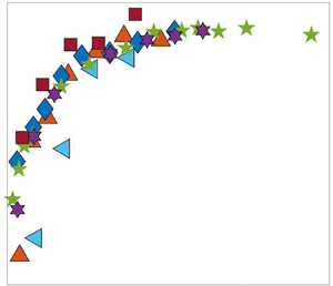
As shown in figure 1(a,c), the critical magnetic Reynolds number is estimated by a linear interpolation between the cases close to the onset of dynamo action. Some additional cases not shown on the plot were also simulated; however, these cases were found to be so close to  $Rm_d$ that the magnetic energy oscillated over a wide range and no clear exponential growth or decay was observed, confirming that our estimated
  $Rm_d$ values are very close to the exact values. The critical magnetic Reynolds number shown in figure 1(a) suggests that
  $Rm_d$ decreases with increasing
  $Pm$; this result is expected and in agreement with previous studies (e.g. Schekochihin et al. Reference Schekochihin, Iskakov, Cowley, McWilliams, Proctor and Yousef2007; Käpylä, Käpylä & Brandenburg Reference Käpylä, Käpylä and Brandenburg2018).

Figure 1. Estimated values of the critical magnetic Reynolds number  $Rm_d$ and the critical Rayleigh number
  $Ra_d$ for the onset of dynamo action. (a) Exponential growth rate
  $(\gamma )$ of magnetic energy versus magnetic Reynolds number
  $(Rm)$. (b) Exponential growth rate
  $(\gamma )$ of magnetic energy versus Rayleigh number
  $(Ra)$. The interpolated critical magnetic Reynolds number
  $(Rm_d)$ and the critical Rayleigh number for dynamo action (
 $Ra_{d}$) for each magnetic Prandtl number
  $(Pm)$ are shown by a ‘
 $\times$’ symbol. (c) Plot of
  $Rm_d$ versus
  $Pm$; and (d) plot of
  $Ra_d$ versus
  $Pm$.
$Pm$.
Bushby et al. (Reference Bushby, Favier, Proctor and Weiss2012) and Käpylä et al. (Reference Käpylä, Käpylä and Brandenburg2018) showed that dynamo action can be excited at a smaller value of  $Rm_d$ with the use of a larger aspect ratio. Käpylä et al. (Reference Käpylä, Käpylä and Brandenburg2018) found that, when
  $Pm = Pr = 1$, an aspect ratio
  $\varGamma \gtrsim 3$ is needed for the growth rate to saturate. In all of our simulations (including those cases with
  $Pr < 1$), an aspect ratio of at least
  $\varGamma \gtrsim 8.5$ is used for the determination of
  $Rm_d$; thus the simulation domain should be sufficiently large to avoid the issue arising from the use of small values of
  $\varGamma$.
While a small subset of simulations were performed with  $Pr=0.01$ and
  $Pr=0.05$, we did not systematically test the role of the aspect ratio for these cases. A single set of tests for
  $Pr=0.05$ (where we increased the aspect ratio
  $\varGamma$ from
  ${\approx }8.5$ to
  ${\approx }14.1$) showed that increasing the aspect ratio did decrease the growth rate. However, the estimated values of
  $Rm_d$ and
  $Ra_d$ were influenced only slightly.
The critical Rayleigh numbers for dynamo action ( $Ra_d$) are estimated using the same procedure as that used for computing
  $Rm_d$. As shown in figure 1(b,d),
  $Ra_d$ decreases as
  $Pm$ is increased. For
  $Pm= (0.8, 1, 3, 5, 7)$ the estimated Rayleigh numbers for the onset of dynamo action are
  $Ra_d= ( 4.9\times 10^5, 2.2\times 10^5, 1.6\times 10^4, 5.2\times 10^3, 3.1\times 10^3)$. As we will show in the following sections, these computed values of
  $Ra_d$ can be useful for collapsing specific data.
A selection of  $Pr=(0.01, 0.05)$ cases with
  $Pm=1$ was also carried out to understand how
  $Pr$ influences dynamo action. Figure 1(a,c) shows that a smaller value of
  $Pr$ yields a lower value of
  $Rm_d$ when
  $Pm$ is held constant. For
  $Pr=(0.01, 0.05, 1)$ with
  $Pm=1$, we find critical magnetic Reynolds numbers of
 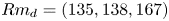 $Rm_d = (135, 138, 167)$. This effect might occur because cases with lower
  $Pr$ (at the same
  $Rm$ and
  $Pm$) tend to have a more coherent flow structure (e.g. Goluskin & Spiegel Reference Goluskin and Spiegel2012; Pandey, Scheel & Schumacher Reference Pandey, Scheel and Schumacher2018; Vogt et al. Reference Vogt, Horn, Grannan and Aurnou2018), which might be more beneficial to dynamo action. At the same
  $Rm$, dynamos with coherent flow are found to have a larger growth rate than dynamos without coherent structures (Tobias et al. Reference Tobias, Cattaneo, Boldyrev, Davidson, Kaneda and Sreenivasan2013). However, a previous study of rotating spherical dynamos suggested that higher values of
  $Rm$ are required for dynamo action if
  $Pr$ becomes too small, though this effect is due to the influence of rotation (Simitev & Busse Reference Simitev and Busse2005). Nevertheless, the Prandtl number appears to play an important role for the onset of small-scale dynamo action; a more systematic investigation, beyond the scope of the present work, is needed to understand this effect in detail.
3.2. Heat transport
In all results presented hereafter, we focus solely on the nonlinear regime of small-scale dynamos. Figure 2(a) shows the Nusselt number ( $Nu$) versus
  $Ra$ for all the cases investigated; the
  $Nu \sim Ra^{2/7}$ scaling is shown for reference. The compensated Nusselt number (
 $Nu/Ra^{2/7}$) is also plotted in figure 2(b). RBC cases without magnetic fields, shown as the black circles, are also plotted for comparison. When the dynamos are activated, the
  $(Nu, Ra)$ curves depart from the RBC scaling. For each value of
  $Pm$, a scaling slope slightly smaller than
  $2/7$ (typically found in RBC at these parameter values) appears. However, as
  $Ra$ is increased further, these slopes appear to approach a
  $2/7$ scaling again, suggesting that the influence of
  $Pm$ on the scaling of
  $Nu$ is weak. For a fixed value of
  $Ra$, the heat transfer is reduced as
  $Pm$ is increased, or, equivalently, as the strength of the magnetic field is increased. Though not shown, the dynamos exhibit similar mean temperature profiles in comparison to RBC, as suggested by the similar heat transport scaling.

Figure 2. Heat transport for all cases: (a) Nusselt number ( $Nu$) versus Rayleigh number (
 $Ra$); and (b) compensated Nusselt number (
 $Nu/Ra^{2/7}$) versus Rayleigh number.
In figure 3 both the viscous dissipation,  $\epsilon _u$, and the ohmic dissipation,
  $\epsilon _B$, are plotted versus the Reynolds number. As suggested in figure 3(a) and the corresponding compensated plot shown in the inset, the viscous dissipation strongly depends on the Reynolds number; a numerical fit of
 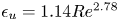 $\epsilon _u =1.14 Re^{2.78}$ is found and shown. We find that the influence of
  $Pm$ on
  $\epsilon _u$ is negligible. A scaling of
  $\epsilon _u \sim Re^{3}$ has been derived for the viscous dissipation in the bulk of the turbulent thermal convection (outside of the boundary layers), while
  $\epsilon _u \sim Re^{5/2}$ has been derived for the boundary layer (Grossmann & Lohse Reference Grossmann and Lohse2000; Scheel & Schumacher Reference Scheel and Schumacher2017). We find that our computed scalings are intermediate between these predicted scalings. Although ohmic dissipation cannot be determined purely by
  $Re$, we observe that, in figure 3(b), ohmic dissipation is approaching the viscous dissipation scaling line as
  $Re$ increases. The compensated plot in figure 3(b) shows the asymptotic scaling behaviour of
  $\epsilon _B \sim Re^{2.78}$ when
  $Re$ is large enough for each individual
  $Pm$. This result suggests that the hydrodynamics properties of the fluid might be controlling both viscous and ohmic dissipation, and inertia appears to play a more important role in the energy cascade than the Lorentz force.

Figure 3. Dissipation for all cases: (a) viscous dissipation  $\epsilon _u$ versus Reynolds number
  $Re$; (b) ohmic dissipation
  $\epsilon _B$ versus
  $Re$; (c) fraction of ohmic dissipation
  $f_{ohm}$ versus
  $Ra$; and (d)
  $f_{ohm}$ versus
  $Ra/Ra_d$, where
  $Ra_d$ is the critical Rayleigh number for dynamo action. A compensated plot is also shown as an inset in panels (a) and (b).
A quantity that provides a useful comparison between viscous and ohmic dissipation is the fraction of ohmic dissipation defined by
 \begin{equation} f_{ohm} \equiv \frac{\epsilon_B}{ \epsilon_u + \epsilon_B }. \end{equation}
Figure 3(c) shows  $f_{ohm}$ versus
  $Ra$ for the dynamo cases. As expected, the flow is dominated by viscous dissipation near the onset of dynamo action. For each value of
  $Pm$,
$Pm$,  $f_{ohm}$ initially increases rapidly with increasing
  $Ra$, but appears to flatten and approaches
  $f_{ohm} \rightarrow 0.5$ as
  $Ra$ is increased. For our most extreme case of
  $Pm=5$ and
 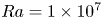 $Ra=1\times 10^7$ (our largest value of Rm), a value of
  $f_{ohm} \approx 0.5$ is reached, suggesting that, in the regime of large
  $Ra$, both ohmic dissipation and viscous dissipation are contributing equally to heat transport.
As shown in figure 3(d),  $f_{ohm}$ (for a given
  $Pr$) collapses when plotted versus the rescaled Rayleigh number
  $Ra/Ra_{d}$, where
  $Ra_{d}$ is the critical Rayleigh number for dynamo action estimated in the previous section. This result suggests that
  $f_{ohm}$ only has a weak dependence on
  $Pm$, while the degree of supercriticality of the Rayleigh number
  $Ra/Ra_{d}$ is playing the dominant role. Similar convergent behaviour of
  $f_{ohm}$ that is weakly dependent on
  $Pm$ was also observed in the hydromagnetic study of Haugen et al. (Reference Haugen, Brandenburg and Dobler2004), although their converged fraction of ohmic dissipation is
  $f_{ohm}\approx 0.7$. We notice that our
  $Pr=0.05$ cases suggest that
  $Pr$ appears not to have a strong influence on the saturated level of
  $f_{ohm}$, though the convergence rates appear to be affected.
Vertical profiles of the horizontally and time-averaged local dissipation  $\epsilon _u(z)$ and
  $\epsilon _B(z)$ are shown in figure 4(a) for a typical dynamo with
  $Pm=5$ and
  $Ra=6\times 10^5$ (
 $Rm = 1122$). Note that here
 \begin{gather} \epsilon_u(z)=\frac{1}{Pm^2} \overline{(\boldsymbol{\nabla}\times \boldsymbol{u})^{2} } , \end{gather}
 \begin{gather}\epsilon_B(z)= \frac{1}{Pm^2} \overline{( \boldsymbol{\nabla}\times \boldsymbol{B})^{2} }. \end{gather}
The ohmic dissipation is dominant near the boundary, while viscous dissipation is dominant in the bulk when  $Rm$ is not too large. We also observe that ohmic dissipation has a markedly thinner boundary layer in comparison to that of the viscous dissipation. Moreover, both profiles show similar structure within the interior, suggesting that both dissipation mechanisms are dynamically linked. The vertical profile of viscous dissipation for the equivalent RBC case is also shown in figure 4(a) for comparison. The viscous dissipation structure of the dynamo remains very similar to that of the RBC case (although their magnitudes are different), suggesting that viscous dissipation has a direct influence on ohmic dissipation in the bulk. The dissipation profiles for our most extreme (largest value of
  $Rm$) dynamo case corresponding to
  $Pm=5$ and
  $Ra=1\times 10^7$ are plotted in figure 4(b). Here the boundary layers become much thinner and the dissipation is dominated by the contribution in the bulk. Again, we find that both profiles show similar structure within the bulk, while the magnitudes are approaching similar values as the Rayleigh number is increased.

Figure 4. Vertical profiles of horizontally and time-averaged viscous dissipation  $\epsilon _u (z)$ and ohmic dissipation
  $\epsilon _B(z)$. (a) Profiles for
  $Pm=5$ and
  $Ra=6\times 10^5$ (
 $Rm \approx 1100$). The corresponding non-magnetic case (RBC) is also plotted for comparison. (b) Profiles for
  $Pm=5$ and
  $Ra=1\times 10^7$ (
 $Rm \approx 3900$). The total dissipation
  $\epsilon _u$ and
  $\epsilon _B$ are calculated by depth averaging the profile.
The behaviour of the dissipation near the boundaries is probably influenced by the choice of boundary conditions. Although we did not perform simulations with no-slip mechanical boundary conditions (as opposed to the stress-free conditions used here), three additional simulations with  $Pm=5$ and
  $Ra= (1\times 10^4, 1\times 10^5, 6\times 10^5)$ were performed in which electrically insulating electromagnetic boundary conditions were used. With these insulating boundary conditions, we found that the depth dependence of the dissipation profiles remained essentially unchanged relative to the vertical magnetic field boundary conditions. Though we found differences in magnitudes of the total dissipation, no systematic variation was investigated. We note that, although the ohmic dissipation tends to be largest near the boundaries, the integrated contribution of this boundary layer region to the total dissipation is relatively small due to the thinness of the layer.
3.3. Flow speeds and energy
Figure 5(a,b) shows the Reynolds number  $Re$ and compensated Reynolds number
  $Re/Ra^{1/2}$ versus
  $Ra$ for all cases. The convective free-fall scaling (
 $Re\sim Ra^{1/2}$) is shown for reference. Curve fits to the data yield
  $Re \sim (Ra^{0.45}, Ra^{0.43}, Ra^{0.43}, Ra^{0.44}, Ra^{0.44})$ for
  $Pr = 1$ and
  $Pm=(0.8,1,3,5,7)$, respectively. We observe that, for the given values of
  $Pr$ and
  $Ra$, the dynamos tend to have smaller flow speeds in comparison to the RBC data, since the magnetic energy comes at the cost of kinetic energy. As
  $Ra$ is increased, the dynamos show a departure from the RBC scaling. The compensated Reynolds number shown in figure 5(b) shows that this departure is very slight, though there is a trend of increased departure with increasing
  $Pm$. The
  $Pr=0.05$ cases show the most rapid growth of
  $Re$ with increasing
  $Ra$, though there are insufficient data to suggest any significant difference in scaling behaviour between the different Prandtl numbers. Despite the fact that approximately half of the dissipation is ohmic (i.e.
  $f_{ohm} \approx 0.4$) for the
  $Pr=0.05$ cases, there is very little difference in flow speeds between the dynamos and RBC. Of course, the Nusselt numbers for these
  $Pr=0.05$ cases are rather small:
  $Nu \lesssim 4$.

Figure 5. Flow speeds for all cases: (a) Reynolds number versus Rayleigh number; and (b) compensated Reynolds number  $(Re/Ra^{1/2})$ versus Rayleigh number.
The efficiency of the dynamos can be measured by the ratio of the magnetic energy to the kinetic energy  $(E_{mag}/E_{kin})$. As shown in figure 6(a), cases with different values of
  $Pm$ show similar behaviour:
  $(E_{mag}/E_{kin})$ increases as
  $Ra$ is increased, and it appears that the ratio approaches constant values at large Rayleigh number. The convergence of the energy ratio was also observed in the mechanically forced dynamo simulations of Haugen et al. (Reference Haugen, Brandenburg and Dobler2004); however, the dependence on magnetic Prandtl number was not discussed. The data can be reasonably collapsed by rescaling the energy ratio with
  $Pm^{2/3}$, and rescaling the Rayleigh number with
  $Ra_d$, as shown in figure 6(b). Since the growth of
  $Re$ depends on
  $Pr$ (e.g. figure 5a,b), we do not expect the
  $Pr=0.05$ data to follow the same trend as the
  $Pr=1$ data. When
  $Ra/Ra_d$ is large enough, dynamos with larger
  $Pm$ can transfer kinetic energy to magnetic energy more efficiently. We note that for
 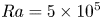 $Ra=5\times 10^5$ and
  $Pm=5$ the energy ratio
  $E_{mag}/E_{kin} \approx 0.2$ agrees with the result of Cattaneo et al. (Reference Cattaneo, Emonet and Weiss2003). Our results suggest that this value represents the approximate asymptote for the energy ratio when
  $Pm=5$, and that the asymptote is
  $Pm$-dependent.

Figure 6. (a) The ratio of magnetic energy to kinetic energy  $(E_{mag}/E_{kin})$ versus the Rayleigh number
  $Ra$. (b) The rescaled energy ratio
  $E_{mag}/(E_{kin} Pm^{2/3})$ versus the rescaled Rayleigh number
  $(Ra/Ra_d)$, where
  $Ra_{d}$ is the critical Rayleigh number for dynamo action.
The magnetic energy is plotted versus Rayleigh number in figure 7(a). The  $E_{mag}\sim Ra$ scaling is shown for reference. The magnetic energy increases relatively rapidly with
  $Ra$ beyond the onset of dynamo action, but appears to flatten and approaches
  $E_{mag}\sim Ra$ at large values of
  $Ra/Ra_d$. Note that, since the energy ratio
  $(E_{mag}/E_{kin})$ saturates at large
  $Ra/Ra_d$, we expect that the magnitude of the magnetic energy must grow with
  $Ra/Ra_d$ at the same rate as the flow speed squared. The compensated magnetic energy (
 $E_{mag}/(Ra\,Pm^{2/3})$) versus the rescaled Rayleigh number
  $Ra/Ra_d$ is shown in figure 7(b). The
  $Pm^{2/3}$ dependence is purely an ad hoc fit to the data and is only meant to provide a rough scaling with
  $Pm$ in the asymptotic regime The curves become relatively flat at large Rayleigh numbers, suggesting that the
  $E_{mag}\sim Ra$ scaling might be an asymptotic result for high-
 $Rm$ RBC dynamos.

Figure 7. Magnetic energy for all cases: (a) magnetic energy versus Rayleigh number; and (b) compensated magnetic energy ( $E_{mag}/(Ra\,Pm^{2/3})$) versus rescaled Rayleigh number
  $Ra/Ra_d$.
3.4. Length scales
The characteristic length scales are computed for all simulations. Two length scales are computed: (i) the Taylor microscale; and (ii) the integral length scale. The Taylor microscale is the length scale at which the influence of viscous or ohmic dissipation becomes important, and can thus provide an estimate for the dissipation length scales. In contrast, the integral scale is the correlation length scale for the corresponding field. The magnetic Taylor microscale  $\lambda _{B}$ and the velocity Taylor microscale
  $\lambda _{u}$ are defined by, respectively,
 \begin{equation} \lambda_{B}=\sqrt{ \frac{\langle {\boldsymbol{B}}^2\rangle }{ \langle (\boldsymbol{\nabla}\times {\boldsymbol{B}})^2\rangle}} \end{equation}
and
 \begin{equation} \lambda_{u}=\sqrt{ \frac{\langle {\boldsymbol{u}}^2\rangle }{ \langle (\boldsymbol{\nabla}\times {\boldsymbol{u}})^2\rangle}}. \end{equation}
Note that these length scales are computed over the entire fluid layer, including the boundary layers. Some tests were done in which the boundary layers were excluded from the calculation, and showed that their influence was negligible. We therefore only present calculations that included the entire fluid layer.
The velocity and magnetic Taylor microscales are plotted versus the Rayleigh number in figure 8(a), which shows in detail how these length scales are modified by  $Pm$. The velocity Taylor microscale
  $\lambda _{u}$ shows very little change with increasing
  $Pm$. Some of the data points show a small increase in
  $\lambda _{u}$ with increasing
  $Pm$; this effect can be understood by the fact that the dynamo converts kinetic energy into magnetic energy and therefore results in a slight decrease of the Reynolds number for a given value of
  $Ra$. However, there is no appreciable difference in the scaling behaviour of
  $\lambda _{u}$ with
  $Ra$ for the various values of
  $Pm$ used here: curve fits to the data yield
  $\lambda _{u} \sim (Ra^{-0.153}, Ra^{-0.171},$
 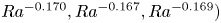 $Ra^{-0.170}, Ra^{-0.167}, Ra^{-0.169})$ for
  $Pm=(0.8,1,3,5,7)$, respectively. The scaling of
  $\lambda _B$ is noticeably steeper than the scaling for
  $\lambda _u$; the corresponding curve fits are
  $\lambda _{B}\sim (Ra^{-0.235}, Ra^{-0.242}, Ra^{-0.245}, Ra^{-0.251}, Ra^{-0.245})$ for
  $Pm=(0.8,1,3,5,7)$, respectively. We emphasize that for all of our simulations we use
  $Pm=O(1)$.

Figure 8. Scaling behaviour of the magnetic Taylor microscale  $\lambda _{B}$ (filled symbols) and velocity Taylor microscale
  $\lambda _{u}$ (empty symbols). (a) Taylor microscale plotted against Rayleigh number. (b) Taylor microscale plotted against Reynolds number. (c) Taylor microscale plotted against magnetic Reynolds number. (d) The rescaled magnetic Taylor microscale
  $(\lambda _{B} Pm^{0.30})$ versus Rayleigh number. (e) The rescaled magnetic Taylor microscale
  $(\lambda _{B} Pm^{0.35})$ (filled symbols) and the velocity Taylor microscale
  $(\lambda _{u})$ (empty symbols) versus the Reynolds number.
Figures 8(b,c) show the velocity and magnetic Taylor microscales versus Reynolds number and magnetic Reynolds number. We observe that  $Pm$ has an influence only on the magnitude of
  $\lambda _{u}$ and
  $\lambda _{B}$; however, the scaling behaviour of these length scales remains basically the same for all
  $Pm$. The scaling
  $\lambda _{B} \sim Rm^{-1/2}$ is also plotted in figure 8(c) for reference. Previous studies of mechanically forced isothermal dynamos suggested that
  $\lambda _{B}$ scales as
  $Rm^{-1/2}$ for fixed
  $Re$ at moderate
  $Rm$ (Brummell et al. Reference Brummell, Cattaneo and Tobias2001). Both results have a
  $\sim Rm^{-1/2}$ dependence; however, we note that they are in a relatively low-
 $Re$ and low-
 $Rm$ regime, and they assume that
  $\lambda _{B}$ does not depend on
  $Re$ and that the magnetic length scale is determined by the balance between advection and diffusion in the induction equation. Our result suggests that
  $\lambda _{B}$ cannot be purely determined by
  $Rm$. As we will show in a later section, there does exist a subdominant balance in the induction equation between induction and diffusion for our cases. Of course, given the very different forcing and boundary conditions between our investigation and that of Brummell et al. (Reference Brummell, Cattaneo and Tobias2001), one might expect differences in the scaling behaviour.
As shown in figure 8(d), the magnetic Taylor microscale collapses when rescaled with  $Pm$; a best fit yields
  $\lambda _{B} Pm^{0.30} = 1.29 Ra^{-0.25}$. Since
  $Re$ scales with
  $Ra$, we also plot the magnetic Taylor microscale as a function of
  $Re$ in figure 8(e), where a scaling law
  $\lambda _{B} Pm^{0.35} = 1.1Re^{-0.56}$ is found. Figure 8(e) shows that the velocity Taylor microscale collapses very well when plotted against
  $Re$, which suggests that the influence of
  $Pm$ on the velocity length scale is very weak, and that the magnetic field has a small effect. Curve fits for all dynamo cases as well as RBC cases yield
  $\lambda _{u}= 0.97 Re^{-0.39}$. For Kolmogorov turbulence, a scaling law of
  $\lambda _{u}\sim Re^{-1/2}$ is obtained (Pope Reference Pope2000). However, dynamos in the RBC geometry cannot be characterized by homogeneous isotropic turbulence, so it is reasonable to expect a modified scaling here. The absence of
  $Pm$ in this scaling law is also expected, as the viscous dissipation appears to be independent of
  $Pm$ within our accessible parameter range.
It is commonly hypothesized that the ohmic dissipation length scale will occur within the inertial range of the turbulence when  $Pm \ll 1$ (
 $Re \gg Rm$) (e.g. Rincon Reference Rincon2019; Tobias Reference Tobias2019). Such a regime requires, at a minimum, that
  $\lambda _B \gg \lambda _u$. Though the simulations in the present study are obviously limited with respect to the accessible parameter range, especially in the restriction to
  $Pm=O(1)$, we observe
  $\lambda _u > \lambda _B$ in all cases. Moreover, the results (especially the
  $Pm=0.8$ cases) shown in figure 8 indicate that the scaling slope (as a function of
  $Ra$,
$Ra$,  $Re$ and
  $Rm$) for the ohmic dissipation length scale is always steeper than the corresponding slope for the viscous dissipation length scale, and that this slope remains mostly independent of
  $Pm$. The case
  $Pm=0.8$ was chosen to allow
  $Pm < 1$, while retaining a sufficiently large
  $Rm$; while this particular case is certainly not a small magnetic Prandtl number, we do not observe a change in the scaling slope with this case relative to
  $Pm \geqslant 1$. Thus, at least for the limited parameter range of the present study, there is no indication that the slopes change drastically either with increasing
  $Ra$ or with decreasing
  $Pm$. However, the
  $Pm$ we explored here are
  $Pm \sim O(1)$, so it remains unclear whether there would be a change in the scaling slope for ohmic dissipation scale when
  $Pm\ll 1$. In that case, we might expect a larger ohmic dissipation scale than the viscous scale.
The depth-dependent integral scales for the magnetic field and velocity field are defined, respectively, by (e.g. Meneguzzi & Pouquet Reference Meneguzzi and Pouquet1989)
 \begin{equation} \ell_B=\frac{\displaystyle\int k^{{-}1} \hat{E}_{mag}(k) \,\textrm{d}k} {\displaystyle\int \hat{E}_{mag}(k) \,\textrm{d}k}, \quad \ell_u=\frac{\displaystyle\int k^{{-}1} \hat{E}_{kin}(k) \,\textrm{d}k} {\displaystyle\int \hat{E}_{kin}(k) \,\textrm{d}k} , \end{equation}
where  $\hat {E}_{mag}(k)$ and
  $\hat {E}_{kin}(k)$ are the magnetic and kinetic energy spectra,
  $\boldsymbol {k} = (k_x,k_y)$ is the horizontal wavenumber vector and
  $k = \sqrt {k_x^2+k_y^2}$. The corresponding depth-dependent Taylor microscales can be computed with the definitions
 \begin{equation} \lambda_{B}' = \left( \frac{\displaystyle\int \hat{E}_{mag}(k) \,\textrm{d}k} {\displaystyle\int k^2 \hat{E}_{mag}(k) \,\textrm{d}k} \right)^{1/2}, \quad \lambda_{u}' = \left( \frac{\displaystyle\int \hat{E}_{kin}(k) \,\textrm{d}k} {\displaystyle\int k^2 \hat{E}_{kin}(k) \,\textrm{d}k} \right)^{1/2}. \end{equation}
We observe a weak dependence on the depth for all of the computed length scales defined above, and therefore only report the depth-averaged values.
The time-averaged values of the spectra-based length scales are calculated for many of the  $Pm=5$ cases. As shown in figure 9, we find nearly identical scaling behaviour between both
  $\lambda _{B}'$ and
  $\lambda _B$, and
  $\lambda _{u}'$ and
  $\lambda _u$. As expected, a divergence between the velocity Taylor microscale and the velocity integral scale occurs as the Reynolds number (Rayleigh number) increases. However, figure 9 also shows that the scale separation for the magnetic field is relatively weak, since the scaling slopes for the two magnetic length scales are close to one another. The integral scale for the velocity appears to be sensitive to the change of aspect ratio (e.g. Stevens et al. Reference Stevens, Blass, Zhu, Verzicco and Lohse2018). As a result, some velocity integral-scale data do appear to follow a clear scaling trend. We should note that the magnetic integral scale appears to have a slope very close to the velocity Taylor microscale, which indicates that there is correlation between the viscous force and the Lorentz force (or magnetic induction).

Figure 9. Depth-averaged length scales for  $Pm=5$: the velocity Taylor microscale
  $(\lambda _{u})$ calculated from energy and dissipation, the velocity Taylor microscale
  $(\lambda _{u}')$ calculated from energy spectra, and the velocity integral scale
  $(\ell _u)$ plotted versus Rayleigh number. The corresponding magnetic length scales are also shown.
3.5. Energy spectra
Figures 10(a,b) show how the kinetic and saturated magnetic energy spectra change with Rayleigh number for  $Pm=5$ dynamos. The
  $\hat {E}_{kin}(k) \sim k ^{-5/3}$ scaling (typically found in the Kolmogorov inertial subrange) is also plotted for reference in figure 10(a), which shows the development of an inertial subrange. The magnetic energy spectra appear to flatten over a large range of wavenumber as
  $Ra$ is increased. For a fixed Rayleigh number, kinetic energy dominates over magnetic energy at large scales. However, for all our (
 $Pm \sim O(1)$) cases, magnetic energy spectra exceed kinetic energy spectra for large wavenumbers. As shown in figure 10(c), the magnetic energy becomes slightly larger than the kinetic energy at small scales, even for the
  $Pm = 0.8$ cases. A
  $k ^{1/3}$ scaling behaviour for the magnetic energy spectra at large scales has been observed in the previous hydromagnetic turbulence study of Haugen et al. (Reference Haugen, Brandenburg and Dobler2004); they also found a
  $k ^{-5/3}$ subrange after the peak of the magnetic energy spectra. These two slopes are plotted in figure 10(b) only for reference, since we do not expect the scalings to be the same for the two different systems. We note that the change in magnetic energy spectra occurs at the wavenumber where the magnitudes of magnetic energy and kinetic energy are comparable. The kinetic energy spectra for RBC (and the
  $k ^{-5/3}$ slope) are also plotted in figure 10(d) for reference. We observe that, when compared with the RBC cases, dynamo action reduces the amplitude of the peak of the kinetic energy spectra and makes the spectra tail less steep. The reduction in the peak amplitude is the result of transferring kinetic energy to magnetic energy by dynamo actions, while the slight increase in the spectra at high wavenumber is due to the Lorentz force driving motion at small scales as
  $Pm > 1$.

Figure 10. Energy spectra: (a) kinetic energy spectra for  $Pm=5$ dynamos; (b) magnetic energy spectra for
  $Pm=5$ dynamos; (c) energy spectra at
  $Ra = 1\times 10^7$ for
  $Pm = 0.8$ (
 $Rm=742$) and
  $Pm = 5$ (
 $Rm=3948$); and (d) kinetic energy spectra for RBC. The spectral slopes of
  $k^{1/3}$ and
  $k^{-5/3}$ are plotted for reference only.
3.6. Forces
In this section we analyse the force balance in the momentum equation to understand the role of the Lorentz force. For the vertical component of the momentum equation, we remove the hydrostatic part by decomposing the flow variables into a horizontal average and a fluctuation. For instance,  $\boldsymbol {u}=\bar {\boldsymbol {U}}+\boldsymbol {u}'$,
  $\boldsymbol {b}=\bar {\boldsymbol {B}}+\boldsymbol {b}'$ and
  $\boldsymbol {\varTheta }=\bar {\boldsymbol {\varTheta }}+\boldsymbol {\theta }'$, where
  $\bar {\boldsymbol {U}}$,
  $\bar {\boldsymbol {B}}$ and
  $\bar {\boldsymbol {\varTheta }}$ are the horizontal mean components,
  $\boldsymbol {u}'$,
  $\boldsymbol {b}'$ and
  $\boldsymbol {\theta }'$ are the fluctuating components, and
  $p'$ is the reduced pressure. Under the present circumstances, we find that the mean components
  $\bar {\boldsymbol {U}}$ and
  $\bar {\boldsymbol {B}}$ are much smaller than the corresponding fluctuating components
  $\boldsymbol {u}'$ and
  $\boldsymbol {b}'$. The fluctuating vertical component of the momentum equation is found by subtracting the mean (hydrostatic) balance to give
 \begin{equation} \underbrace{\partial_t w' }_{F_t}= \underbrace{ Pm\nabla^2 w'}_{F_v} + \underbrace{(-\boldsymbol{u}'\boldsymbol{\cdot}\boldsymbol{\nabla}w' +\partial_z\overline{w'^2})}_{F_a} + \underbrace{Pm(\boldsymbol{b}'\boldsymbol{\cdot}\boldsymbol{\nabla}b_z' -\partial_z\overline{b_z'^2})}_{F_l} + \underbrace{\frac{Ra\,Pm^2}{Pr}\theta' }_{F_b} -\underbrace{ {\partial_z} p'}_{F_p}. \end{equation}
We use the same symbols for denoting the various terms in the horizontal components of the momentum equation.
The time-averaged root-mean-squared (r.m.s.) values of the different terms in the momentum equation are calculated at the midplane ( $z=0.5$) and shown in figure 11(a,b). The vertical dependence of the forces was also analysed using vertical profiles as in Yan et al. (Reference Yan, Calkins, Maffei, Julien, Tobias and Marti2019), and it was found that the data shown in figure 11(a,b) were representative of all depths. The Lorentz force initially grows rapidly with increasing
  $Ra$, then slows once it becomes comparable in magnitude with the viscous force. We note that, even for the largest value of
  $Ra$, the Lorentz and viscous forces are approximately the same magnitude. We observe that the time derivative term (inertia) grows at the fastest rate with increasing
  $Ra$ among all terms in the horizontal components of the momentum equation. The corresponding forces for RBC (without magnetic field) are plotted in figure 11(c,d) for comparison. We observe that the scaling of the buoyancy force is basically the same for both the dynamo and RBC, whereas the scaling slopes for all other forces in the dynamos are reduced relative to RBC.

Figure 11. Time-averaged r.m.s. values of forces in the momentum equation at the midplane ( $z=0.5$) for (a,b) dynamos with
  $Pm=5$ and (c,d) RBC. (a,c) Forces in the horizontal direction versus Rayleigh number. (b,d) Forces in the vertical direction versus Rayleigh number. Advection and the Lorentz, viscous, buoyancy, pressure gradient and inertia forces are denoted by
  $F_a$,
  $F_l$,
  $F_v$,
  $F_b$,
  $F_p$ and
  $F_t$, respectively.
Horizontal spectra are computed for all forces in the momentum equation at the midplane, and are shown in figure 12(a) for  $Pm=5$ dynamo and in figure 12(b) for RBC at
  $Ra=6 \times 10^5$. A convective free-fall balance in which the pressure gradient force, buoyancy force and advection are comparable is present at the largest spatial scales (smallest wavenumbers) for both cases. For the dynamo, the Lorentz force is subdominant at large spatial scales (
 $k \lesssim 70$), and is in a near-perfect balance with the viscous force at small spatial scales (
 $k \gtrsim 40$). The spectra of the sum of the Lorentz force and the viscous force are calculated and plotted as the dashed line. At small scales, the sum of the two forces is one order of magnitude smaller than both Lorentz force and viscous force, suggesting that there is an almost exact balance between Lorentz force and viscous force locally. Part of the velocity driven by the Lorentz force is dissipated by viscosity locally and almost instantaneously. This result suggests that the viscous length scale might be controlling the magnetic field length scales, which explains the similar scaling slopes for the velocity Taylor microscale and the magnetic integral scale. A similar argument for the balance between the viscous force and the Lorentz force was also discussed in previous studies (Brummell et al. Reference Brummell, Cattaneo and Tobias2001; Schekochihin et al. Reference Schekochihin, Maron, Cowley and McWilliams2002c), and our spectral result serves as direct evidence for this local balance. Note that the spectra we show here are for
  $Pm=5$ cases. For small
  $Pm$, it is possible that the Lorentz force might behave quite differently at small scale, though in all of our cases we find that the Lorentz force is driving the flow at small scale. When compared with the RBC case of figure 12(b), broader spectra are observed for the dynamo case; advection, viscous and inertia forces are slightly reduced at large scales and larger in magnitude at small scales, which suggests that the Lorentz force is consuming kinetic energy at large scales while driving the flow at small scales.

Figure 12. Horizontal spectra of the various forces in (a) dynamo with  $Pm=5$ and (b) RBC. For both cases
  $Ra=6\times 10^5$. (c) Lorentz force and viscous force spectra for
  $Pm=5$ dynamos.
Figure 12(c) shows the Lorentz force and viscous force spectra for  $Pm=5$ dynamos at
  $Ra=(4\times 10^4, 2\times 10^5, 6\times 10^5, 1\times 10^6)$. Initially (
 $Ra\sim 4\times 10^4$), the Lorentz force is weaker than the viscous force at large scales, and is in balance with the viscous force at small scales. When
  $Ra$ increases, the Lorentz force exceeds the viscous force at large scales; this result is also reflected in the relatively rapid initial growth of
  $F_l$ in figure 11(a,b). However, as
  $Ra$ is increased further (
 $Ra > 2\times 10^5$), the growth of the Lorentz force at large scales appears to slow down; both the Lorentz force and the viscous force spectra appear to shift to larger wavenumber, and the length scale where the two forces are balanced becomes smaller. We note that the spectra of the Lorentz force appear to flatten and saturate at small wavenumber as
  $Ra$ is increased. This result suggests that the Lorentz force might be limited by the viscous force (at least at small length scales), and the growth rate of the Lorentz force appears to saturate.
3.7. Induction equation balances
Analogous to the force balance analysis of the momentum equation in the previous section, here the relative sizes of the different terms in the magnetic induction equation are analysed in both physical and spectral space. Figures 13(a–d) show vertical profiles of the instantaneous horizontal r.m.s. of each term in the induction equations, for two typical cases, both with  $Ra=10^6$, and with
  $Pm = 1$ and
  $Pm=5$, respectively; these cases correspond to magnetic Reynolds numbers of
  $Rm\approx 310$ and
  $Rm \approx 1340$. Though not shown, cases with different values of
  $Pm$ and
  $Ra$ show similar behaviour. Not surprisingly, given that
  $Rm\gg 1$, the primary balance indicates that advection of magnetic field dominates,
 \begin{equation} {\partial_t} \boldsymbol{B} + {\boldsymbol{u}} \boldsymbol{\cdot}\boldsymbol{\nabla} \boldsymbol{B} \approx 0. \end{equation}
In addition, a subdominant balance is observed between magnetic induction and magnetic diffusion,
 \begin{equation} {\boldsymbol{B}}\boldsymbol{\cdot} \boldsymbol{\nabla} \boldsymbol{u} \sim \nabla^2 \boldsymbol{B}. \end{equation}
We also find that the magnitude of  $\partial _t \boldsymbol {B}+\boldsymbol {u} \boldsymbol {\cdot } \boldsymbol {\nabla } \boldsymbol {B}$ is of the same order as induction and diffusion.

Figure 13. Instantaneous balances in the induction equation. Vertical profiles of the horizontal r.m.s. of each term present in the vertical component (a,b) and in the horizontal component (c,d) of the induction equation and the corresponding power spectra (of all three components) at the midplane (e,f) are shown. The case  $Pm=1$ and
  $Ra=1\times 10^6$ is shown in (a,c,e). The case
  $Pm=5$ and
  $Ra=1\times 10^6$ is shown in (b,d,f ). Magnetic induction, diffusion, advection and time derivative are denoted by
  $\boldsymbol {B}\boldsymbol {\cdot }\boldsymbol {\nabla }\boldsymbol {u}$,
  $-\boldsymbol {u}\boldsymbol {\cdot }\boldsymbol {\nabla }\boldsymbol {B}$,
  $\nabla ^2\boldsymbol {B}$ and
  $\partial _t \boldsymbol {B}$. Finally,
  $w$ and
  $B_z$ represent the vertical component of
  $\boldsymbol {u}$ and
  $\boldsymbol {B}$, while
  $u_h$ and
  $B_h$ represent the vertical component.
The depth dependence of the different terms is similar for the two different cases shown. Interestingly, even though  $Rm$ is approximately an order of magnitude larger for the
  $Pm=5$ case, the relative difference in magnitude between the leading-order balance and the subdominant balance changes only slightly; for instance,
  $|{\boldsymbol {u}} \boldsymbol {\cdot } \boldsymbol {\nabla } \boldsymbol {B}|/|\nabla ^2 \boldsymbol {B}| \approx 3$ and
  $|{\boldsymbol {u}} \boldsymbol {\cdot } \boldsymbol {\nabla } \boldsymbol {B}|/|\nabla ^2\boldsymbol {B}| \approx 4$ for
  $Pm=1$ and
  $Pm=5$, respectively. This result could be due to the small-scale magnetic Reynolds number not changing appreciably.
The spectral space representation of the different terms in the induction equation is given in figure 13(e,f) for the same  $Ra=10^6$,
  $Pm=1$ and
  $Pm=5$ cases, respectively. Again, the data are computed at one instant in time. Whereas
  ${\partial _t} \boldsymbol {B}$ and
  ${\boldsymbol {u}} \boldsymbol {\cdot } \boldsymbol {\nabla } \boldsymbol {B}$ are balanced at all length scales, the stretching (
 ${\boldsymbol {B}} \boldsymbol {\cdot } \boldsymbol {\nabla } \boldsymbol {u}$) and diffusion (
 $\nabla ^2 \boldsymbol {B}$) terms are balanced at different length scales. This scale-dependent balance can be understood by a simple scale analysis of the subdominant balance. For instance, (3.10) yields
 \begin{equation} \frac{Rm}{L_u} \sim \frac{1}{L_B^2}, \end{equation}
where the velocity has the non-dimensional units of magnetic Reynolds number,  $L_u$ is a characteristic length scale for the velocity and
  $L_B$ is a characteristic length scale for the magnetic field. Since the magnetic length scale is in the diffusion term (
 $\nabla ^2 \boldsymbol {B}$), it is natural to assume that this length scale can be captured by the magnetic Taylor microscale
  $L_B = \lambda _B$. Thus we have
 \begin{equation} Rm \sim \frac{L_u}{\lambda_B^2}. \end{equation}
 However, it is not obvious what  $L_u$ represents. We plug in the magnetic Taylor microscale
  $(\lambda _{B})$ and test the velocity Taylor microscale
  $(\lambda _{v})$ as well as the velocity integral scale
  $(\ell _u)$; the results are shown in figure 14. We find that, when using the velocity Taylor microscale
  $(\lambda _{v})$, the curve for the compensated magnetic Reynolds number
  $Rm \, \lambda _{B}^2 /\lambda _{u}$ is relatively flat; however, we can still see a systematic increase of
  $Rm\,\lambda _{B}^2 /\lambda _{u}$ with increasing
  $Ra$. When we apply the velocity integral scale
  $\ell _u$, the compensated magnetic Reynolds number
  $Rm \,\lambda _{B}^2 /\ell _u$ stays nearly constant over a large range of
  $Ra$, suggesting that the velocity integral scale
  $\ell _u$ can better characterize the length scale in the induction terms than the Taylor microscale. This result implies that the magnetic diffusion length scale is controlled by
  $Rm$ and the velocity integral scale:
 \begin{equation} Rm \sim \frac{\ell_u}{\lambda_B^2}. \end{equation}
Figure 14. Rescaled magnetic Reynolds number versus Rayleigh number for  $Pm = 5$ cases. Both
  $Rm\,\lambda _{B}^2 /\lambda _{u}$ and
  $Rm\,\lambda _{B}^2 /\ell _u$ results are shown.
4. Discussion
RBC-driven dynamos have been investigated numerically over a range of Rayleigh numbers and magnetic Prandtl numbers. Heat transport in dynamos is reduced relative to RBC, primarily because of the associated reduction in kinetic energy required for the generation of magnetic energy. Simulations at the largest values of  $Ra$ suggest a heat transport scaling with
  $Ra$ that is similar to RBC, i.e.
  $Nu \sim Ra^{2/7}$ within our investigated range of
  $Ra$. The scaling behaviour of the flow speeds with increasing Rayleigh number is also similar to RBC (
 $Re \sim Ra^{1/2}$). An asymptotic scaling for the magnetic energy
  $E_{mag} \sim Ra$ is also observed at large
  $Ra/Ra_d$. Given a large enough value of
  $Ra/Ra_d$, the ratio of magnetic energy to kinetic energy
  $E_{mag}/E_{kin}$ appears to saturate for individual
  $Pm$, while the saturated level depends on
  $Pm$; we find reasonable collapse of the data using
  $E_{mag}/E_{kin} \sim Pm^{2/3}$. This result suggests that
  $Pm$ is controlling the efficiency of dynamo action.
Despite the similar scaling behaviour in  $Nu$ for both RBC and RBC-driven dynamos, for a fixed value of
  $Pm$, the simulations show that ohmic dissipation becomes as equally important as viscous dissipation as the Rayleigh number increases, as characterized by an ohmic dissipation fraction
  $f_{ohm} \rightarrow 0.5$. The scaling of the viscous dissipation in the dynamos is observed as
  $\epsilon _u \sim Re^{2.8}$, which is nearly identical to equivalent RBC simulations (Grossmann & Lohse Reference Grossmann and Lohse2000). Moreover, the ohmic dissipation is observed to approach the scaling
  $\epsilon _B \sim Re^{2.8}$ as
  $Ra$ is increased. The findings suggest that ohmic dissipation is controlled by viscous dissipation.
The Taylor microscale is computed for both the velocity field and magnetic field, thus providing a measure of the viscous and ohmic dissipation scales, respectively. The ohmic dissipation scale is observed to be smaller than the viscous dissipation scale for all simulations, even for the  $Pm=0.8$ cases. Furthermore, the ohmic dissipation length scale decreases more rapidly with increasingly Rayleigh number (Reynolds number) in comparison to the viscous dissipation length scale. Curve fits yield scalings of
  $\lambda _{B} \sim Re^{-0.56} Pm^{-0.35}$ and
  $\lambda _{u} \sim Re^{-0.39}$ for velocity field and magnetic field Taylor microscale, respectively. Unless a change in scaling occurs at higher Rayleigh numbers beyond those accessible in the present study, this result suggests that the ohmic dissipation scale is always less than the viscous dissipation scale, regardless of the value of the magnetic Prandtl number for the values of
  $Pm$ considered in this paper.
A numerical analysis of the forces in both physical and spectral space shows that the viscous and Lorentz forces are in balance at small spatial scales. The viscous force in dynamos is enhanced at these same scales relative to RBC. At large spatial scales, the Lorentz force dominates the viscous force, but it remains subdominant relative to buoyancy and inertia. A two-dimensional (in the horizontal plane) spectral energy analysis suggests that the Lorentz force is primarily dissipative at large spatial scales, but acts as a source of kinetic energy at small spatial scales; this result might explain why the viscous force at small spatial scales is enhanced in dynamos relative to RBC.
To leading order, the induction equation is characterized by a conservation of magnetic flux. Stretching and diffusion act at higher order and are dominant at large and small spatial scales, respectively. According to this balance, the magnetic diffusion length scale is found to be related to the magnetic Reynolds number and velocity integral scale via  $\lambda _B \sim (\ell _u/ Rm)^{1/2}$.
In light of the limited range in Rayleigh numbers accessible to DNS studies of dynamos, several questions remain. Since the buoyancy force has a relatively smaller growth rate with increasing  $Ra$ when compared to that of the Lorentz force, it remains unclear whether the growth of the Lorentz force will slow down and approach the scaling of the buoyancy force when
  $Ra$ becomes large enough, or if the Lorentz force will eventually dominate over the buoyancy force and change the dynamics fundamentally. Simulations with higher
  $Ra$ are also needed to verify the asymptotic convergence behaviour of flow speeds, magnetic energy and dissipation. For planetary interiors and stars, the thermal Prandtl number is less than unity, and the dependence of the magnetic energy to kinetic energy ratio and the ohmic dissipation fraction on
  $Pr$ remain unclear and might also need to be explored in more detail.
We reiterate that all of the simulations presented here use  $Pm = O(1)$. In the small-
 $Pm$ regime in which
  $Pm \ll 1$, one might expect the stretching of the eddies to be balanced by magnetic diffusion on the ohmic dissipation length scale (Rincon Reference Rincon2019; Tobias Reference Tobias2019). Although the low-
 $Pm$ regime is currently beyond the reach of DNS, our results (especially the
  $Pm = 0.8$ and
  $Pm=1$ cases) suggest that, instead of a sudden change at
  $Pm = 1$, the transition to the low-
 $Pm$ regime might be gradual, or occur sharply at much lower
  $Pm$. This observation is consistent with calculations (Tobias, Cattaneo & Boldyrev Reference Tobias, Cattaneo and Boldyrev2012) that suggest numerical resolutions of
  $(10^4)^3$ modes are required to reach this large-
 $Re$ regime. Further investigation with smaller
  $Pm$ will therefore be needed to explore the mechanisms that drive the changes between the scalings.
Acknowledgements
This work utilized the RMACC Summit supercomputer, which is supported by the National Science Foundation (awards ACI-1532235 and ACI-1532236), the University of Colorado–Boulder and Colorado State University. The Summit supercomputer is a joint effort of the University of Colorado–Boulder and Colorado State University. The authors acknowledge the Texas Advanced Computing Center (TACC) at The University of Texas at Austin for providing high-performance computing resources that have contributed to the research results reported within this paper.
Funding
This work was supported by the National Science Foundation under grant EAR *1620649 (to M.Y. and M.A.C.). S.M.T. would like to acknowledge support from the European Research Council (ERC) under the European Union's Horizon 2020 research and innovation programme (Agreement No. 328D5S-DLV-786780).
Declaration of interests
The authors report no conflict of interest.
Appendix
The details of our numerical simulations are listed in tables 1–5.
Table 1. Details of the numerical simulations for  $Pr = 1$ and
  $Pm = (0.8, 1, 3)$ cases. The non-dimensional parameters are the Rayleigh number
  $Ra$, the Prandtl number
  $Pr$, the magnetic Prandtl number
  $Pm$, the aspect ratio of the domain
  $\varGamma = {2 {\rm \pi}n}/{k_c}$, the Nusselt number
  $Nu$, the Reynolds number
  $Re$, the magnetic Reynolds number
  $Rm$ and the magnetic energy
  $E_{mag}$. The spatial resolution is quoted in terms of the dealiased physical space grid points
  $N_x \times N_y \times N_z$, where
  $(N_x,N_y)$ is the horizontal resolution and
  $N_z$ is the vertical resolution. The numerical time-step size is denoted by
  $\Delta t$. The estimated critical Rayleigh numbers for dynamo action (
 $Ra_d$) are
  $(4.9\times 10^5, 2.2\times 10^5, 1.6\times 10^4)$ for
  $Pm = (0.8, 1, 3)$, respectively.

Table 2. Details of the numerical simulations for  $Pr = 1$ and
  $Pm = (5, 7)$ cases. The estimated critical Rayleigh numbers for dynamo action (
 $Ra_d$) are
  $(5.2\times 10^3, 3.1\times 10^3)$ for
  $Pm = (5, 7)$, respectively.

Table 3. Details of the numerical simulations for  $Pr = 0.05$ and
  $Pm = 1$ cases. The estimated critical Rayleigh numbers for dynamo action (
 $Ra_d$) are
  $(2.9\times 10^3, 4.1\times 10^3)$ for
  $Pm = 1$,
  $Pr = (0.01, 0.05)$, respectively.

Table 4. Details of the RBC cases.

Table 5. Details of the numerical simulations used for the kinematic dynamo regime. The growth (or decay) rate of magnetic energy is denoted by  $\gamma$.


