


1. Introduction
To tackle the challenges posed by climate change, global policies increasingly advocate for a significant rise of renewable sources within the energy mix. In this context, the wind energy sector has shown an exceptional growth, raising problems related to the sizing, positioning and operation of wind turbines. The trade-off between technical constraints and resource availability usually results in wind turbines being densely grouped in clusters known as wind farms, whose efficiency largely depends on the so-called wake interactions. Wind power extracted by a wind turbine is intimately related to its drag coefficient  $C_D$ defined as follows:
 \begin{equation} C_D = \frac{F_D}{\dfrac{1}{2}\rho U_\infty^2 A}, \end{equation}
where  $F_D$ is the drag force experienced by the body,
  $\rho$ is the air density,
  $U_\infty$ is the incoming velocity and
  $A$ is the frontal area of the body. Since
  $C_D$ is intimately linked to wake recovery, accurately predicting the development of wind-turbine wakes is crucial for optimising wind farm operation. However, the number of degrees of freedom characterising this problem is so vast that it is currently extremely challenging to solve it with standard high-fidelity numerical tools. To overcome this issue, simplified approaches are required. A popular example of this strategy is the actuator disc concept first introduced by Rankine (Reference Rankine1865), which assimilates the wind-turbine rotor to a porous medium surrogate across which a pressure drop can be tuned to match the drag coefficient (Van-Kuik et al. Reference Van-Kuik, Sørensen, Nørkær and Okulov2015).
At the laboratory scale, the actuator disc concept has been implemented using porous discs to mimic isolated wind turbines (see e.g. Aubrun Reference Aubrun2013; Howland et al. Reference Howland, Bossuyt, Martinez-Tossas, Meyers and Maneveau2016) or wind farms (see e.g. Camp & Cal Reference Camp and Cal2016; Bossuyt, Meneveau & Meyers Reference Bossuyt, Meneveau and Meyers2017; Stevens, Martínez-Tossas & Meneveau Reference Stevens, Martínez-Tossas and Meneveau2018). As a starting point, the seminal work of Castro (Reference Castro1971) on perforated flat plates, later on extended by Steiros & Hultmark (Reference Steiros and Hultmark2018), emphasise the attractiveness of this analogy reducing the problem complexity to a single physical parameter: the porosity  $\beta$, which represents the ratio of empty volume to total volume. Based on potential flow theory and conservation laws, Steiros & Hultmark (Reference Steiros and Hultmark2018) derived a relationship between
  $C_D$ and
  $\beta$, which was successfully validated against experimental measurements for any porosity value. This means that tuning the porosity of a porous disc is a simple and efficient way to match the drag coefficient of a wind turbine, while keeping the global dimensions (i.e. the diameter of the area swept by the rotor) constant. By doing so, some physics of the mean wake of a wind turbine can be reproduced at low costs in a laboratory setting, even if it does not generate power from the wind (Aubrun Reference Aubrun2013). For instance, Sforza, Sheerin & Smorto (Reference Sforza, Sheerin and Smorto1981) studied experimentally the wake generated by porous discs within various operating conditions. Aubrun (Reference Aubrun2013) conducted an experimental survey comparing the wake generated by a laboratory-scale rotating wind turbine with that of a porous disc. Analysing mean velocity and turbulence intensity profiles, these authors concluded that, beyond 3 rotor diameters, both wakes behave similarly. Identical conclusions were reached by Stevens et al. (Reference Stevens, Martínez-Tossas and Meneveau2018), who investigated the influence of the wind-turbine model incorporated in large eddy simulations for both a single wind turbine and a wind farm. Comparing their results with the experimental database reported by Chamorro & Porte-Agel (Reference Chamorro and Porte-Agel2011), these authors showed that the actuator disc model is well adapted to capture the main features of the mean wake.
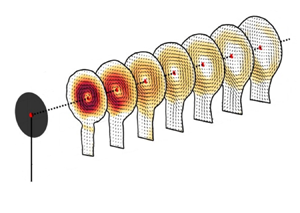
As depicted in figure 1, the porous disc model has shown an evolution throughout the years marked by a shift in focus towards porosity distribution – from models with uniform porosity (Sforza et al. Reference Sforza, Sheerin and Smorto1981; Aubrun Reference Aubrun2013; Lignarolo, Ragni & Ferreira Reference Lignarolo, Ragni and Ferreira2016) to those featuring a non-uniform porosity distribution (Camp & Cal Reference Camp and Cal2016; Howland et al. Reference Howland, Bossuyt, Martinez-Tossas, Meyers and Maneveau2016; Helvig et al. Reference Helvig, Vinnes, Segalini, Worth and Hearst2021). The progression toward increasingly intricate designs, with the aim of more accurately mirroring the blades of a wind turbine, is evident. Recently, Aubrun et al. (Reference Aubrun2019) and Vinnes (Reference Vinnes2023) performed a detailed comparison of both types of porosity distribution in different facilities. The authors found discrepancies from flow to flow that they attributed to variations in the initial conditions of the wake, which are known to have a very long-range influence (Bevilaqua & Lykoudis Reference Bevilaqua and Lykoudis1978; Wygnanski, Champagne & Marasli Reference Wygnanski, Champagne and Marasli1986). This observation resonates with the results reported by Stevens et al. (Reference Stevens, Martínez-Tossas and Meneveau2018), who showed that adding more details to the initial conditions of the actuator disc model (like the nacelle, hub and mast) greatly increased its fidelity. This tends to show that by restricting the design of the actuator disc concept to a single parameter, porosity, the relevance of this model is likely to remain limited.

Figure 1. Schematic diagram showing the chronology of the porous disc model used as a wind-turbine surrogate for wind-tunnel experiments and corresponding references.
Camp & Cal (Reference Camp and Cal2016) pointed out that, although the porous disc model can closely approximate most statistics of the mean flow, it inherently lacks the ability to replicate swirl, which is a defining feature in the near wake of wind turbines (Porté-Agel, Bastankhah & Shamsoddin Reference Porté-Agel, Bastankhah and Shamsoddin2020). This additional motion comes from the rotation of the blades, which confer an angular momentum to the wake. Knowing that swirl plays a crucial role in areas like combustion (Masri, Kalt & Barlow Reference Masri, Kalt and Barlow2004) and geophysics (Moisy et al. Reference Moisy, Morize, Rabaud and Sommeria2011), its omission in the design of actuator disc may result in oversimplified wind-turbine surrogate. In fact, professor Joukowsky (Reference Joukowsky1912) had already emphasised the relevance of rotation in screw vortex systems like propellers, helicopters and wind turbines (readers interested in Joukowsky's legacy to the development of rotor theory are referred to Okulov, Sørensen & Wood (Reference Okulov, Sørensen and Wood2015) and Van-Kuik et al. (Reference Van-Kuik, Sørensen, Nørkær and Okulov2015)). Introducing the swirl number  $F_D \mathcal {L}/G_0$, where
  $\mathcal {L}$ is a characteristic length scale (typically the rotor diameter) and
  $G_0$ is the axial flux of angular momentum (Oberleithner et al. Reference Oberleithner, Sieber, Nayeri, Paschereit, Petz, Hege, Noack and Wygnanski2011), Reynolds (Reference Reynolds1962) investigated the self-similar solutions by considering two asymptotic cases: linear momentum (drag) dominated flows, i.e.
  $F_D \mathcal {L}/G_0 \gg 1$, and angular momentum (swirl) dominated flows, i.e.
  $F_D \mathcal {L}/G_0 \ll 1$. While the latter regime is reminiscent of wakes behind self-propelled bodies (Chernykh, Demenkov & Kostomakha Reference Chernykh, Demenkov and Kostomakha2005), the former regime corresponds to the framework in which most popular wake recovery models were established (Jensen Reference Jensen1983; Frandsen et al. Reference Frandsen, Barthelmie, Pryor, Rathmann, Larsen, Højstrup and Thøgersen2006; Bastankhah & Porté-Agel Reference Bastankhah and Porté-Agel2014). Recently, Holmes & Naughton (Reference Holmes and Naughton2022) estimated a range of swirl number values for real wind turbines using the results from the National Renewable Energy Laboratory's FAST8 wind-turbine model (Bortolotti et al. Reference Bortolotti, Tarres, Dykes, Merz, Sethuraman, Verelst and Zahle2019). Swirl numbers reaching values up to 0.25 (i.e.
  ${O}(1)$) were found, meaning that the influences of both linear and angular momentum are significant and cannot be disregarded. In this scenario, the consideration of swirl becomes indispensable in accurately predicting wind-turbine wake development.
The objective of this investigation is twofold and is based on the following two questions: How can a porous disc generate a swirling wake while maintaining its simplicity? What is the influence of swirl on the structure and the development of the wake? The latter question underscores the primary focus of the paper, which is to examine the influence of swirl on the self-similar behaviour of the wake. While the studies by Wosnik & Dufresne (Reference Wosnik and Dufresne2013) and Holmes & Naughton (Reference Holmes and Naughton2022) offer valuable insights into the classical similarity analysis of swirling wakes, based on the approaches of Tennekes & Lumley (Reference Tennekes and Lumley1972), Townsend (Reference Townsend1976) and George (Reference George1989), recent advancements in turbulence theory (see Seoud & Vassilicos Reference Seoud and Vassilicos2007; Nedic Reference Nedic2013; Dairay, Obligado & Vassilicos Reference Dairay, Obligado and Vassilicos2015; Vassilicos Reference Vassilicos2015) provide an opportunity to revisit self-similar analysis of the swirling wake without relying on restrictive assumptions about the nature of turbulence in the flow. The outline of the paper is therefore structured as follows: § 2 examines the theoretical implications of considering swirl in the development of a turbulent axisymmetric wake with particular attention to the similarity analysis; § 3 describes the porous disc design process to passively include swirl and presents the experimental set-up. The aerodynamic performances of the proposed porous disc is assessed in § 4, which is completed by a mean wake survey in § 5, where a scaling analysis is conducted. Conclusions are drawn in § 6 along with some perspectives.
2. Self-similarity analysis of the mean swirling wake
In this section, the scaling laws of the main parameters featuring a swirling wake are derived based on a self-preserving approach. To this end, simplified conservation laws are first established. Then, different scenarios are explored depending on the state of the dissipation rate of turbulent kinetic energy. As illustrated in figure 2, we consider an axisymmetric wake generated by an actuator of diameter  $D$ centred at the origin of the cylindrical coordinates system (
 $x, r, \phi$). The swirling motion of the wake is triggered by an angular momentum
  $G_0$ injected to the flow at the actuator disc location. The wake is characterised by its velocity components
  $u$,
$u$,  $v$ and
  $w$ along the streamwise (
 $x$), the radial (
 $r$) and the azimuthal (
 $\phi$) directions, respectively. The actuator disc is subjected to an inflow characterised by a free-stream velocity
  $U_\infty$. For the remainder of the paper, the symbol
  $\bullet ^\star$ denotes normalised quantities using
  $U_\infty$ and
  $D$ as characteristic scales for velocities and lengths, respectively.

Figure 2. Schematic diagram of the axisymmetric swirling wake generated by an actuator disc contained in a control volume  $\mathcal {V}$. Here,
  $U$ and
  $W$ are the mean streamwise and azimuthal components, respectively,
  $P_\infty$ is the free-stream static pressure and
  $n_i$ are the outbound vectors normal to the surfaces.
2.1. Governing equations and relevant simplifications
Since the theoretical framework describing the development of axisymmetric free shear flows has been established by previous works (see e.g. Townsend Reference Townsend1976; George Reference George1989; Johansson, George & Gourlay Reference Johansson, George and Gourlay2003; Shiri, George & Naughton Reference Shiri, George and Naughton2008), we will only give a brief review of the main equations on which the self-similar analysis is based. Under the boundary-layer approximation (i.e.  $\partial /\partial r \gg \partial /\partial x$), the mean momentum transport equation along the streamwise direction is the following:
 \begin{equation} U\frac{\partial U}{\partial x} + V\frac{\partial U}{\partial r} ={-} \frac{1}{r}\frac{\partial (r\overline{u'v'})}{\partial r} + \frac{\partial}{\partial x} \left\{ \overline{v'^2}-\overline{u'^2} + \int_r^\infty\frac{W^2 + (\overline{w'^2}-\overline{v'^2})}{r'}\,{\rm d}r' \right\}, \end{equation}
where  $U$,
$U$,  $V$ and
  $W$ are the mean velocity components, while
  $u'$,
$u'$,  $v'$ and
  $w'$ represent the turbulent fluctuations along the streamwise (
 $x$), the radial (
 $r$) and the azimuthal (
 $\phi$) directions, respectively. The symbol
  $\bar {\bullet }$ stands for the ensemble averaging operator. Note that, in this expression, the streamwise pressure gradient is inferred via the mean momentum transport equation along the radial direction leading to the term in brackets (Shiri et al. Reference Shiri, George and Naughton2008). Equivalently, the mean momentum transport equation along the azimuthal direction reads
 \begin{equation} U\frac{\partial W}{\partial x} + V\frac{\partial W}{\partial r} +\frac{V W}{r} ={-}\frac{\partial \overline{v'w'}}{\partial r} -2\frac{\overline{v'w'}}{r} - \frac{\partial \overline{u'w'}}{\partial x}. \end{equation}
Integrating (2.1) over a control volume  $\mathcal {V}$ encompassing the actuator disc (see figure 2) leads to the following expression:
 $$\begin{gather} C_D = \frac{2 F_D}{\rho U_\infty^2 A_{{disc}}} = 16 \underbrace{\int_0^\infty U^*\Delta U^* r^*\,{\rm d}r^*}_{\text{I}} - 16 \underbrace{\int_0^\infty\left[\overline{u'^2}^* - \frac{\overline{w'^2}^* + \overline{v'^2}^*}{2}\right]r^*\,{\rm d}r^*}_{\text{II}} \nonumber\\ +\, 16 \underbrace{\int_0^\infty \left[ \frac{W^{*^2}}{2} \right] r^*\,{\rm d}r^*}_{\text{III}}, \end{gather}$$
where  $\rho$ is the working fluid density,
  $A_{{disc}} = {\rm \pi}D^2/4$ the surface area of the actuator disc,
  $F_D$ its aerodynamic drag and
  $\Delta U = U_\infty - U$ the velocity defect. Here,
  $F_D$ acts as a body force, representing the external force term from the wind turbine. Equation (2.3) relates the drag coefficient
  $C_D$ to the mean momentum deficit flow rate (term I), the turbulence anisotropy (term II) and the mean kinetic energy of swirl (term III). Our measurements emphasise that term
  $I$ predominates in (2.3) which reduces to
 \begin{equation} C_D \approx 16\int_0^\infty U^\star \Delta U^\star r^\star \,{\rm d}r^\star. \end{equation}
In the same manner, an angular momentum budget using (2.2) applied on the control volume  $\mathcal {V}$ yields
 \begin{equation} G_0^\star= \frac{2 G_0}{\rho U_\infty^2 A_{{disc}} D} = 16 \int_0^\infty \left( U^\star W^\star+ \overline{u'w'}^\star\right) r^{{\star}^2}\,{\rm d}r^\star, \end{equation}
which expresses that the integrated angular momentum remains constant along the streamwise direction and is equal to its source value. Here again, our measurements show that the transport of angular momentum by the Reynolds shear stress (i.e.  $\overline {u'w'}^\star$) is marginal compared with that transported by the mean swirling motion (i.e.
  $U^\star W^\star$) in the examined region of the flow. Equation (2.5) thus reduces to
 \begin{equation} G_0^\star\approx 16 \int_0^\infty U^\star W^\star r^{{\star}^2} \,{\rm d}r^\star. \end{equation}
The validity of these approximations is discussed in more detail in Appendix A, where the contribution of the omitted terms is quantified. It should be noted that the conservation laws (2.4) and (2.6) are valid asymptotically for the far-wake region of the flow but are useful to establish compelling phenomena in more intermediate regions of the flow. These laws govern the evolution of the mean swirling wake as it develops in the streamwise direction and are at the basis of the self-preservation analysis conducted in the following part.
2.2. Similarity analysis
In this section, we revisit the self-similar analysis of the swirling wake conducted by Wosnik & Dufresne (Reference Wosnik and Dufresne2013), and extend it to the non-equilibrium turbulence paradigm (Vassilicos Reference Vassilicos2015). The similarity analysis consists in seeking self-similar solutions for the flow properties which have to satisfy the conservation laws (2.4) and (2.6). Following Townsend (Reference Townsend1976) and George (Reference George1989), these conservation laws act as the ‘similarity constraints’, which allow us to establish the so-called ‘intermediate asymptotics’ (Cantwell Reference Cantwell1978; Barenblatt Reference Barenblatt1996). To this end, we assume that any flow variable can be expressed as  $\bullet (x,r) = \bullet _s(x) f(\zeta )$, where
  $\bullet _s$ represents the typical amplitude of the variable,
  $f$ is a self-similar function and
  $\zeta = r/\delta (x)$, with
  $\delta (x)$ a characteristic length of the flow. An important remark regarding the choice of
  $\delta$ has to be made here. Since the evolution of classical axisymmetric wakes is solely governed by the linear momentum conservation law (2.4), it is natural to choose a characteristic length directly connected to the velocity deficit
  $\Delta U$. For that reason,
  $\delta$ is most often assimilated to the wake half-width
  $\delta _{1/2}$, which is by definition
  $\Delta U(x, r=\delta _{1/2}) = U_s(x)/2$, where
  $U_s(x)$ is the maximum velocity deficit at the streamwise location
  $x$ (Pope Reference Pope2000). Unlike classical axisymmetric wakes, however, the swirling wake features an additional constraint in the form of the conservation of mean angular momentum (2.6). This introduces an additional characteristic length scale
  $\delta _{swirl}$ to the similarity analysis linked to the swirling velocity such that
  $W(x,r=\delta _{swirl}) = W_s(x)$, where
  $W_s(x)$ is the characteristic swirl amplitude at the streamwise location
  $x$. The way both
  $\delta _{swirl}(x)$ and
  $W_s(x)$ are estimated is detailed in § 4 of the manuscript and illustrated in figure 10. In other words, the way the swirling wake develops will depend on the competition between the linear and angular momenta. In contrast to the analysis of Wosnik & Dufresne (Reference Wosnik and Dufresne2013), we assume in the following that the wake in the vicinity of the actuator disc is a region of the flow governed by the swirling motion. Moreover, no assumption is made about the dissipation scaling law, i.e. whether it be based on equilibrium or non-equilibrium turbulence.
Substituting self-similar forms in the conservation laws (2.4) and (2.6) and assuming that the porosity of the actuator disc is high enough so that  $U^\star \approx 1$, we get
 $$\begin{gather} C_D \sim \left[ U_s^\star \delta^{{\star}^2} \right] \int_0^\infty \zeta g(\zeta) \,{\rm d}\zeta, \end{gather}$$
 $$\begin{gather}G_0^\star\sim \left[ W_s^\star \delta^{{\star}^3} \right] \int_0^\infty \zeta^2 h(\zeta) \,{\rm d}\zeta, \end{gather}$$
where  $g$ and
  $h$ are similarity functions. Given that the linear and angular momenta remain constant and equal to their source values, the products in square brackets in the previous equations are also constant, which implies that
 $$\begin{gather} U_s^\star\sim \delta^{{\star}^{{-}2}}, \end{gather}$$
 $$\begin{gather}W_s^\star\sim \delta^{{\star}^{{-}3}}. \end{gather}$$
Using (2.9) and (2.10) yields  $U_s \sim W_s^{2/3}$, a relationship that is well supported by the data reported in Wosnik & Dufresne (Reference Wosnik and Dufresne2013). As discussed in Townsend (Reference Townsend1976) and in George (Reference George1989), a final step is then necessary to close the system. To this end, the transport equation of the turbulent kinetic energy is used, providing an additional constraint relating the expansion rate of the characteristic length scale
  $\delta$ to the turbulent dissipation rate
  $\epsilon$ and reads
 \begin{equation} \frac{{\rm d}\delta}{{\rm d}\kern0.7pt x} \sim \frac{\epsilon \delta}{U_s^2 U_\infty}. \end{equation}
A general expression for  $\epsilon$ was proposed by Vassilicos (Reference Vassilicos2015) and specifically applied by Dairay et al. (Reference Dairay, Obligado and Vassilicos2015) to derive non-equilibrium scaling laws for axisymmetric wakes. It reads
 \begin{equation} \epsilon = C_\epsilon \frac{U_s^3}{\delta}, \end{equation}
with  $C_\epsilon \sim Re_D^m / Re_\ell ^n$, where
  $Re_D = U_\infty D / \nu$ and
  $Re_\ell = U_s \delta / \nu$ represent global and local Reynolds numbers, respectively. Note that, while the integral length scale and the square root of the turbulent kinetic energy at a centreline location
  $\sqrt {K_0(x)}$ were originally used as characteristic scales, Dairay et al. (Reference Dairay, Obligado and Vassilicos2015) outlines how (2.12) is adapted for the similarity analysis of wakes. The nature of the turbulence is then controlled by the exponents
  $m$ and
  $n$. Following Dairay et al. (Reference Dairay, Obligado and Vassilicos2015), the classical equilibrium turbulence (in the Kolmogorov sense) is retrieved by imposing
  $m=n=0$, which yields
  $C_\epsilon = \mbox {const}$, while non-equilibrium turbulence corresponds to the condition
  $m=n=1$. Coupling (2.11) and (2.12) yields
 \begin{equation} \frac{{\rm d}\delta^\star}{{{\rm d}\kern0.7pt x}^\star} \sim Re_D^{m-n} \frac{U_s^{{\star}^{1-n}}}{\delta^{{\star}^{n}}}. \end{equation}
Taking  $n=m=0$, (2.13) becomes
  ${\rm d}\delta ^\star /{{\rm d}\kern0.7pt x}^\star \sim U_s^\star$, meaning that the expansion rate scales linearly with the velocity deficit. Substituting (2.9) into (2.13) yields the classical so-called Townsend (Reference Townsend1976) and George (Reference George1989) scalings
 \begin{equation} \delta^\star\sim (x^\star - x_0^\star)^{1/3} \quad \text{and} \quad U_s^\star\sim (x^\star- x_0^\star)^{{-}2/3}, \end{equation}
where  $x_0$ stands for a virtual origin. Accounting for (2.10), it immediately follows that
 \begin{equation} W_s^\star\sim (x^\star - x_0^\star)^{{-}1}. \end{equation}
This scaling law, which dictates the decay of the swirl amplitude, was initially established by Wosnik & Dufresne (Reference Wosnik and Dufresne2013). However, the authors noticed that this prediction was not well supported by their experimental data. They argued that this departure from the predicted law might have been related to the presence of tip vortices. Recently, Holmes & Naughton (Reference Holmes and Naughton2022), who studied the axisymmetric swirling wake of a rotating porous disc at different rotation speeds, claimed that the equilibrium scaling laws predicted the swirl decay rate only after an ‘initial adjustment region’. In other words, Wosnik & Dufresne (Reference Wosnik and Dufresne2013) as well as Holmes & Naughton (Reference Holmes and Naughton2022) evidenced that equilibrium similarity fell short in accurately predicting swirl decay in the intermediate wake region. In fact, recent findings suggest that non-equilibrium regions are found in turbulent wakes and hold over a large span of streamwise distances from the wake generator and even at very far distances (Nedic Reference Nedic2013; Dairay et al. Reference Dairay, Obligado and Vassilicos2015).
Accordingly, considering now the non-equilibrium framework, i.e.  $n=m=1$, (2.13) becomes
  ${\rm d}\delta ^\star /{{\rm d}\kern0.7pt x}^\star \sim \delta ^{\star ^{-1}}$, which implies
 \begin{equation} \delta^\star\sim (x^\star - x_0^\star)^{1/2}. \end{equation}
Note that neither of the similarity constraints (2.9) nor (2.10) were invoked to obtain (2.16). This means that, with a non-equilibrium approach, the nature of the length scale  $\delta$ is not implicitly attributed either to the velocity deficit or the swirling motion. Instead,
  $\delta$ is directly related to the mechanism which sets the level of dissipation in the turbulent wake. Injecting (2.16) into (2.9) and (2.10) yields
 \begin{equation} U_s^\star\sim (x^\star - x_0^\star)^{{-}1}, \end{equation}
and
 \begin{equation} W_s^\star\sim (x^\star - x_0^\star)^{{-}3/2}. \end{equation}
This novel non-equilibrium scaling law (2.18) predicts a faster decay of swirl amplitude when compared with its equilibrium counterpart. Naturally, this theoretical law needs to be confronted with data for validation. In this work, an experimental wind-tunnel approach was privileged. The following section will therefore provide a comprehensive description of the experimental set-up used to generate and characterise the swirling wake of a modified actuator disc.
3. Experimental set-up
3.1. Design of the porous discs with passive swirl generation
The actuator discs used in this study have been designed based on the work of Helvig et al. (Reference Helvig, Vinnes, Segalini, Worth and Hearst2021), who investigated the wake generated by porous discs featuring various porosity patterns. Here, following the nomenclature proposed by Helvig et al. (Reference Helvig, Vinnes, Segalini, Worth and Hearst2021), a scaled-up version of their non-uniform holes disc with 35 % solidity (referred to as NHD35 in Helvig et al. Reference Helvig, Vinnes, Segalini, Worth and Hearst2021) has been selected as a reference. The main geometrical parameters and dimensions of the porous discs are shown in figure 3. The porous discs have a diameter and a thickness of  $D = 100$ mm and
  $e = 5$ mm, respectively. Each porous disc has a central solid disc of
  $25$ mm in diameter with a
  $6$ mm hole in the middle. From this solid disc, 16 trapezoidal blades make up the body of the disc along with an inner rim that is
  $61$ mm in diameter and
  $1.5$ mm in width. The outer rim of the porous disc is
  $2$ mm wide. Following Camp & Cal (Reference Camp and Cal2016) and Helvig et al. (Reference Helvig, Vinnes, Segalini, Worth and Hearst2021), the number of blades and their size are the main factors which can be adjusted to obtain the desired porosity, noted
  $\beta$, defined as
 \begin{equation} \beta = \frac{A_h}{A_{{disc}}}, \end{equation}
where  $A_{h}$ is the empty area of the trapezoidal holes. While the local porosity varies along the radial direction, the global porosity of the disc is
  $\beta =65\,\%$, matching exactly the NHD35 disc studied in Helvig et al. (Reference Helvig, Vinnes, Segalini, Worth and Hearst2021). The porous discs were designed with a commercial three-dimensional design software (ANSYS™ SpaceClaim) and printed in polylactic acid using a Cura™ Ultimaker 3 Extended printer.

Figure 3. The NHD35 porous disc (a) global parameters (front and side view) and (b) isometric view.
In contrast to the approach taken by Holmes & Naughton (Reference Holmes and Naughton2022), we chose to introduce the swirling motion in a passive manner by slightly modifying the disc's geometry. This methodology is illustrated schematically in figure 4. It consists in pitching the trapezoidal blades that come out from the centre of the disc of an angle  $\alpha >0^{\circ }$. The main interest of this approach is to keep the design stage simple and inexpensive. However, this method lacks pre-defined control over the level of injected swirl and must be therefore estimated a posteriori. Nevertheless, some predictions for the swirl amplitude as a function of
  $\alpha$ can be made by assimilating each individual blade to a thin flat plate of infinite span for which the thin airfoil theory (Anderson Reference Anderson2011) predicts a lift coefficient
  $C_L = 2{\rm \pi} \alpha$, with
  $\alpha$ expressed in radians, as depicted in figure 5. Besides, according to the Kutta–Joukowski theorem, for non-stalled blades, the lift coefficient per unit span can be expressed as a function of the circulation
  $\varGamma$ such as
  $C_L = 2\varGamma ^\star /e^\star$, where
  $e^\star$ is assimilated to the dimensionless blade chord. Since the inclination of the blades is what induces the swirling motion, the circulation per unit span is intimately related to the swirling velocity such as
  $\varGamma \sim W_s \ell$ where, by definition,
  $\ell$ is the typical extent of the contour integral on which the circulation is computed. It comes naturally that
  $\ell = {\rm \pi}D/n$, where
  $n$ is the number of blades of the porous disc, which leads to
 \begin{equation} C_L \sim \left(\frac{2{\rm \pi}}{n}\right) \frac{W_s^\star}{e^\star}. \end{equation}
Therefore, the amplitude of the swirling motion featured by  $W_s^\star$ scales linearly with the lift coefficient per unit span
  $C_L$ according to potential flow theory. Replacing the expression for the lift coefficient derived from thin airfoil theory in (3.2) yields
 \begin{equation} W_s^\star\sim n e^\star \alpha = 0.8 \alpha, \end{equation}
which predicts a linear increase of the swirl magnitude with respect to the pitch angle  $\alpha$. The slope of (3.3) sets the theoretical upper limit for the generation of swirl until stall appears. Due to finite size blade effects, non-constant aspect ratio of the blades and their surface finish, a lower slope is expected. As shown in figure 5, there is a critical pitch angle
  $\alpha _c$ beyond which stall appears. This will result in a decrease in lift, consequently reducing the swirl intensity according to (3.2). The value of
  $\alpha _c$ depends on several parameters (e.g. Reynolds number, surface roughness, aspect ratio
 $\ldots$), making it difficult to accurately predict. However, based on experimental data reported in the literature, a discernible range can be defined for flat plates with comparable average aspect ratios, as highlighted by Nakayama (Reference Nakayama1988); Mohebi, Wood & Martinuzzi (Reference Mohebi, Wood and Martinuzzi2017), this range is
  $\alpha _c \in [14^{\circ }\unicode{x2013}20^{\circ }]$. To tackle this issue, a parametric study has been conducted by varying the pitch angle
  $\alpha$ within the range
  $[5^{\circ }\unicode{x2013}30^{\circ }]$. Moreover, the appearance of massive flow separation over the blades will diminish the effective porosity of the actuator disc, leading to an increase in its drag. To evaluate this effect, supplementary discs with thicker, but not pitched, blades were manufactured. For those discs, the blade thickness was chosen such that their frontal area matches the projected area of an original blade at a specific pitch. These low-porosity discs have been manufactured to be compared with pitched discs at
  $\alpha = 15^{\circ }$ and
  $\alpha = 25^{\circ }$. Alternative porous disc designs featuring curved blades, rather than straight pitched blades, were tested to passively generate swirl. While this approach generated stronger swirl, it also resulted in increased drag. This design was ultimately set aside due to the added complexity it introduced to the study and its impact on the disc's drag coefficient. The three-dimensional models of the porous discs used in this work are available upon request.

Figure 4. Modification of the porous discs to generate a swirling wake showing a frontal view of (a) the  $\alpha = 0 ^{\circ }$ reference case, (b) a porous disc with pitched blades (
 $\alpha >0 ^{\circ }$) and (c) an unfolded view of the modifications. Black dashed lines: zoomed-in area.

Figure 5. Schematic of the influence of the pitch angle  $\alpha$ on the lift coefficient experienced by the blades of the porous disc to passively add swirl. The thin airfoil theory prediction is symbolised by the red dashed line. The vertical black dot-dashed line represents the critical angle at which stall occurs. Unfolded views are provided to illustrate the flow path through the actuator disc with different scenarios: (
 $\blacksquare$, red) blades with no pitch, (
 $\bigstar$, blue) blades with a pitch angle in the pre-stall regime and (
 $\bullet$, green) with a pitch angle in the post-stall regime.
3.2. Wind tunnel and test rig implementation
The experiments were conducted in the S2 subsonic, Eiffel type, open-circuit wind tunnel of the PRISME Laboratory at the University of Orléans. The test section is 2 m long with a cross-sectional area of  $0.50\times 0.50\,{\rm m}^2$ with walls entirely made of Plexiglas to allow for optical access. The free-stream velocity
  $U_\infty$ can reach
  $50\,{\rm m}\,{\rm s}^{-1}$, while the background turbulence intensity remains lower than
  $0.35\,\%$. This laminar inflow type was specifically selected to isolate and assess the impact of swirl on wake development. While a more realistic representation of wind-turbine wakes would account for external turbulence to capture interactions with the atmospheric boundary layer, this falls outside the scope of the current study. For details regarding the effects of external turbulence, we refer readers to studies such as Gambuzza & Ganapathisubramani (Reference Gambuzza and Ganapathisubramani2023).
The implementation of the porous discs in the wind tunnel is depicted in figure 6. The discs are fixed on a T-shaped aluminium cylindrical rod with a diameter  $d = 6$ mm representing the wind-turbine nacelle and tower. The hub can be assimilated to the central solid disc where the disc is fixed to the rod (figure 3). With this set-up, the porous discs were interchangeable without the need to remove the rod, ensuring that our data would not be affected by an eventual misalignment between experiments. The wind-tunnel blockage ratio is approximately
  $2\,\%$ (rod included), ensuring a relatively undisturbed wake. Accordingly, no blockage correction was applied. The test rig is mounted to an aerodynamic balance placed below the wind tunnel floor. The origin of the coordinates is located at the cross-roads between the mast and the nacelle rod. The
  $x$-axis corresponds to the streamwise direction, the
  $y$-axis to the spanwise direction and the
  $z$-axis to the vertical direction.

Figure 6. (a) Front view of the test rig and (b) schematic of the experimental set-up (not to scale). Green boxes: particle image velocimetry (PIV) fields of view, magenta solid lines: maps in  $y$–
$y$– $z$ planes, dotted red lines: vertical (
 $z$) profiles, blue squares: horizontal (
 $y$) profiles (three-component hot-wire anemometry, 3CHWA).
3.3. Metrology and methodologies
The measurement tools used in this work were selected to assess the conservation laws and similarity analysis established in § 2. Accordingly, the drag force experienced by the porous disc has to be measured to obtain direct values of  $C_D$. Besides, three-component velocity measurements are needed to fully characterise the wake evolution.
3.3.1. Drag force measurements
In order to determine the drag coefficient  $C_D$ of each porous disc, an ATI™ Mini40-E balance was used. Placed directly beneath the wind tunnel floor, this balance is capable of measuring force and torque components in all three directions (
 $x,y,z$). Since the entire test rig is attached to the Mini40-E attach point, the balance provides measurements of the test rig's total drag
  $F_x^{TR}$. To isolate the drag experienced by the porous disc from that generated by the mast (excluded from our definition of
  $C_D$), we followed the method proposed in Helvig et al. (Reference Helvig, Vinnes, Segalini, Worth and Hearst2021). It consists in performing drag measurements of the T-shaped rod alone,
  $F_x^{rod}$, and subtracting them from the test rig's total drag, giving thereby a surrogate for the porous disc drag following
  $F_D = F_x^{TR} - F_x^{rod}$. For the
  $\alpha =0^{\circ }$ case, the value of
  $F_x^{TR}/F_x^{rod}$ is 5. This indicates that the rod contributes 20 % of the total drag. Note that this method introduces errors to the drag measurements of the porous discs due to the interactions between the disc and the rod. However, the assumption is made that this interaction remains the same for all pitch angles. The sampling frequency was set to 1 kHz and the measurement duration was
  $180$ s. A moving average on 100 samples was used to filter out the vibrations, resulting in an effective sampling frequency of
  $10$ Hz. The uncertainties were estimated using the calibration errors (
 ${\pm }1.5\,\%$ of the measured load) and the statistical errors. The statistical errors were determined using the standard deviation of the force signal. The uncertainties amounted to
  $\epsilon _{C_D}=0.03$ on average. It was found that, beyond
  $Re_D \approx 10^5$,
  $C_D$ becomes Reynolds number independent. Therefore, in the remainder of this paper, we report only results obtained at
  $Re_D = 1.3 \times 10^5$, which corresponds to a free-stream velocity of
  $U_\infty = 20\,{\rm m}\,{\rm s}^{-1}$.
3.3.2. Three-component hot-wire anemometry
To measure the swirling wake, 3CHWA measurements were conducted using a Dantec Dynamics™ Streamline constant temperature anemometry system with a gold-plated tungsten tri-axial wire probe (Dantec Dynamics™ 55P91 probe). The probe has three gold-plated tungsten wires having a diameter of  $5\,\mathrm {\mu }{\rm m}$, an individual wire sensing length of 1.2 mm and a total sensing length of 3.2 mm, which is of the order of the Taylor microscale
  $\lambda \in [2 ; 4] \,{\rm mm}$ (Sreenivasan, Prabhu & Narasimha Reference Sreenivasan, Prabhu and Narasimha1983; Mora et al. Reference Mora, Pladellorens, Turró, Lagauzere and Obligado2019). The probe was subjected to a directional calibration before each campaign and to a velocity calibration between measurements. This specific probe has a maximum yaw angle range of
  $[-30^{\circ } ; +30^{\circ }]$ beyond which velocity measurements are erroneous. The hot-wire anemometry (HWA) measurements were used to estimate the characteristic scales of the turbulent flow, which are reported in table 1. The estimated scales are:
  $\mathcal {L}_{int}$ the integral length scale,
  $\lambda$ the Taylor microscale,
  $\eta$ the Kolmogorov length scale and
  $\mathcal {T}_{int}=\mathcal {L}_{int}/U$ the integral time scale. In particular, the integral length scale was calculated at each available position by integrating the autocorrelation function of the streamwise velocity fluctuations until its first zero crossing. This approach was confronted with other methods such as the one described in Mora & Obligado (Reference Mora and Obligado2020). The estimated error from the discrepancies between these methods remained below 6 % beyond
  $x=3D$ for all cases. As shown in figure 7, cross-sectional planes were measured at three streamwise positions:
  $x=2D$,
  $x=4D$ and at
  $x=6D$. The number of measurements points is
  $N_p=1130$. The spatial resolution is
  $\Delta y_{wake} = \Delta z_{wake} = 5$ mm (
 ${\approx }2\lambda$) inside the wake and 10–20 mm (
 ${\approx }\mathcal {L}_{int}$) in the free stream (figure 7). Spanwise and vertical profiles were measured between
  $X=2D$ and
  $X=6D$ with a streamwise step of
  $\Delta _x=0.5D$. The sampling frequency was set to
  $40$ kHz for an acquisition time of
  $2.5$ s (
 ${\sim }10^3 \mathcal {T}_{int}$) at each location. Streamwise profiles (
 $y^\star =z^\star =0$) were also measured from
  $x^\star =1$ to
  $x^\star =7$. The trade-off of using a three-component probe was the reduction in the spatial resolution due to its size, which affects the estimation of dissipation rate
  $\epsilon$. In this study, we use a formulation based on local isotropy and Taylor's hypothesis to compute
  $\epsilon _{iso}=15\nu \overline {(\partial u^\prime _x /\partial x )^2}$, a surrogate commonly employed in the literature. Hereinafter, a detailed analysis is carried on two distinct configurations: the swirling case with
  $\alpha =25^{\circ }$ (65 % porosity) and its non-swirling counterpart with reduced porosity. These configurations are selected as they represent the conditions where probe resolution is most critical. Additionally, measurements are taken at several key locations along the centreline (
 $z^\star =0$), the top edge of the disc (
 $z^\star =0.5$) and the bottom edge of the disc (
 $z^\star =-0.5$). It is important to note that the use of this approach, although common, must be made with care as the assumptions on which it is based are far from fully validated in the present case. For this reason, a concurrent approach was also used to estimate the dissipation rate. This second method is based on zero crossings to estimate the Taylor microscale from which the dissipation rate can be computed (Rice Reference Rice1944, Reference Rice1945; Liepmann & Robinson Reference Liepmann and Robinson1952; Sreenivasan et al. Reference Sreenivasan, Prabhu and Narasimha1983; Mazellier & Vassilicos Reference Mazellier and Vassilicos2008; Goto & Vassilicos Reference Goto and Vassilicos2009). This technique was used in a number of flows (jet, grids and so-called ‘chunk’ turbulence) and is notably less sensitive to the probe resolution with respect to the Kolmogorov scale
  $\eta$, as evidenced by Mazellier & Vassilicos (Reference Mazellier and Vassilicos2008). Indeed, it relies on an inner cutoff scale
  $\eta ^\star$ which is found to be approximately 60 times larger than
  $\eta$. This implies that the probe resolution is around
  $0.25\eta ^\star$, making it well suited to estimating the zero-crossing-based dissipation rate
  $\epsilon _{zc}$. Note that, while the study of Mazellier & Vassilicos (Reference Mazellier and Vassilicos2008) covered a broad range of turbulent flows, wakes were not part of the dataset. The variation of
  $\epsilon _{zc}$ compared with its isotropic counterpart
  $\epsilon _{iso}$ is displayed in figure 8. It appears that the uncertainties remain within 20 % whatever the operating conditions and the probe location. Although encouraging, these results are not entirely satisfactory due to the shortcomings of the methods used. For this reason, the results obtained on dissipation must be regarded qualitatively rather than quantitatively. To fully validate the results reported for dissipation, more experiments are needed comparing data using a higher resolution hot-wire probe at different locations of the wake for example. Future work could also consider a different experimental approach using high resolution PIV where the dissipation rate can be accurately estimated when properly denoised, as reported in Chen et al. (Reference Chen, Cuvier, Foucaut, Ostovan and Vassilicos2021). Based on this analysis, we report
  $\epsilon _{iso}$ as the dissipation rate throughout the remainder of the paper.
Table 1. Typical turbulent length and time scales calculated in the wake of the different porous discs at  $x^\star =6, y^\star = z^\star =0$.


Figure 7. The 3CHWA measurement points. Grey disc: porous disc position, solid black line: cylindrical mast.

Figure 8. Comparison between the zero-crossing-based dissipation rate  $\epsilon _{zc}$ and the surrogate estimated from the local isotropy assumption
  $\epsilon _{iso}$ for different configurations (3CHWA). Vertical dashed line: position from which the wake is analysed.
During the HWA measurements, the main uncertainty sources came from the inherent changes in the experimental conditions (temperature, humidity, pressure) and from the calibration of the hot-wire probe (Duffman Reference Duffman1980; Bruun Reference Bruun1996). The total uncertainty in the free-stream was below 0.5 % and around 0.8 %–2 % in the wake depending on the position of the probe with respect to the test rig. The temperature of the room was monitored throughout each experiment and was shown not to exceed a variation of more than  $1\,^\circ {\rm C}$ for all cases. The HWA uncertainties were estimated between experiments using the calibration unit and corroborated by redundant measurements. Following (2.4) and to better assess the effect of swirl on the flow, the streamwise velocity component had to be measured with a better spatial resolution and accuracy than what is achievable with HWA. Therefore, PIV measurements were performed in the streamwise plane.
3.3.3. Particle image velocimetry over multiple fields of view
Planar PIV (PIV2D2C) was used to characterise the generated wakes in an  $x$–
$x$– $z$ plane (figure 6). In the streamwise direction, the region of interest is located between
  $x=-2D$ and
  $x=8D$. This region is decomposed into 3 separate fields of view (FoVs) with an overlapping area of 25 % (
 $1D$). The dimensions of the individual FoVs are (
 $x \times z$)
  $4.2D\times 2.6D$ and the full region reaches
  $10D \times 2.6D$. The total region was obtained by merging the mean velocity fields and standard deviations using a similar approach to that proposed in Li et al. (Reference Li, Zhao, Liu and Carmeliet2021). The image sets were captured using an 11 megapixels LaVision™ LX-11M CCD camera mounted on an optical rail parallel to the test section. A ZEISS™ camera lens was used with focal length
  $f_0 = 85$ mm and was set at an aperture of
  $f_0/4$. The flow was illuminated using a double pulse Nd:YAG (532 nm) laser system generating a laser sheet of 1.5 mm thickness. The flow was seeded with olive oil droplets from an aerosol generator and had an average diameter of
  $d_p\approx 2\unicode{x2013}3\,\mathrm {\mu }{\rm m}$. Olive oil droplets were chosen as tracers since they are non-reactive, non-toxic, scatter light appropriately and are sufficiently small in order to faithfully represent the fluid motion. To prove this last important point, the average Stokes number
  $St$ was calculated using all scales of motion and showed that
  $St \in [1 ; 40] \times 10^{-3} \ll 1$. The generated tracer particles will therefore follow all scales of motions reliably (Kallio & Stock Reference Kallio and Stock1992; Vincent Reference Vincent2007).
For each FoV, 2600 image pairs were recorded at a time interval of  $dt = 55\,\mathrm {\mu }{\rm s}$ between snapshots. The sampling frequency was set at
  $f_{PIV}=2.1$ Hz, a rate which corresponds to a total acquisition time of
  $T_{PIV} = 24$ min. The laser pulses and the frame recordings were synchronised using an external LaVision™ programmable timing unit. The snapshots were analysed using a commercial PIV software (Davis 10.2, LaVision™). A multi-pass cross-correlation method was applied using an initial interrogation window (IW) size of
  $64\times 64$ pixels and a final IW of
  $32\times 32$ with 50 % overlap (Raffel, Willert & Kompenhans Reference Raffel, Willert and Kompenhans2007). A Gaussian filter was used for sub-pixel interpolation and a median filter was applied in order to remove eventual spurious vectors.
Each FoV required an individual calibration. The calibration was performed using a custom calibration plate with uniformly spaced dots. The plate is 540 mm long and 420 mm tall and has a total of 560 dots ( $28 \times 20$) which are 4 mm in diameter and 19.45 mm apart. The calibration plate was placed in the mid-span plane of the test section next to the test rig. The resulting calibrations allowed each FoV to have a magnification factor (pixels to mm) and to correct optical aberrations (Raffel et al. Reference Raffel, Willert and Kompenhans2007). The magnification factor had a constant value of
  $SF=9.61\,{\rm pixels}\,{\rm mm}^{-1}$ for each calibration. The PIV algorithm resulted in a resolution of
  $\Delta _x^{{PIV}} = \Delta _z^{{PIV}} = 1.66 \,{\rm mm}$, which is of the order of the Taylor microscale
  $\lambda$ and 10 times smaller than the integral length scale
  $\mathcal {L}_{int}$ (see table 1).
Uncertainties for the PIV measurements were calculated using correlation statistics, a method presented in Wieneke (Reference Wieneke2015) and applied here. This method estimates PIV uncertainties based on a pixel-wise statistical analysis that quantifies the contribution of each pixel to the shape of the correlation peak. The error quantification method resulted in a displacement uncertainty of  $\epsilon _d \in [0.03 ; 0.08]$ px, which range falls within the order of magnitude of the 0.06 px value recommended in Raffel et al. (Reference Raffel, Willert and Kompenhans2007). As a side note, the error shoots up to values of
  $\epsilon _d \approx 0.15\unicode{x2013}0.20$ px very close to the test rig, which is expected since strong three-dimensional effects are present and increase the noise due to out-of-plane motion. Moreover, the swirling cases will increase this out-of-plane motion by definition. This error was quantified and corresponds to an instantaneous velocity uncertainty of 0.8 % and a mean uncertainty below 0.5 % in the wake of the porous discs. It was verified that the flow statistics converged properly beyond 2000 snapshots.
4. Modified porous disc aerodynamics
This section is devoted to a parametric study of how the pitch angle  $\alpha$ affects the aerodynamics of the porous discs presented in the previous section, with reference to the unmodified porous disc for which
  $\alpha =0^{\circ }$. First, the evolution of swirl characteristics with respect to
  $\alpha$ is examined, from which two distinct operating regimes are highlighted. Then, the drag and the swirl number induced by the modified discs are analysed in detail with the aim of distinguishing the effects of porosity and swirl.
4.1. Characteristics of the swirling motion
Let us start by assessing the level of swirling motion injected in the wake of the modified porous discs. Figure 9 shows the streamwise evolution ( $x^\star = 2$, 4 and 6) of the dimensionless mean swirling velocity
  $W^\star$ for
  $\alpha = 15^{\circ }$ and
  $\alpha = 25^{\circ }$ in comparison with the porous disc with non-pitched blades. For the latter, it is evident that the swirling motion is marginal, aside from a small area where the wake of the disc merges with that of the mast. This is likely due to three-dimensional effects in this wake interaction region. Furthermore, the absence of swirl for the reference case confirms that the porous disc is properly aligned with the direction normal to the incoming flow. As evidenced in figure 9(c–h), incorporating a pitching angle yields the generation of a swirling motion whose distribution is toroidal. Moreover, the swirl intensity decays as the streamwise distance from the disc increases. Besides, its distribution spreads radially as a consequence of the conservation of the initial angular momentum.

Figure 9. Normalised swirling velocity  $W^\star$ spanwise maps (3CHWA) for the (a,b)
  $\alpha =0^{\circ }$ case, (c–e) the
  $\alpha =15^{\circ }$ case and ( f–h) the
  $\alpha =25^{\circ }$ case evaluated at
  $x^\star =2$ (a,c, f),
  $x^\star =4$ (d,g) and at
  $x^\star =6$ (b,e,h). Solid blue line: contour of the porous disc, dashed blue line: cylindrical mast.
To further characterise the swirling motion, it is essential to derive physical parameters that represent the swirl intensity and its spatial distribution, i.e.  $W_{s}$ and
  $\delta _{swirl}$, respectively. As illustrated in figure 10, these quantities are inferred from spanwise profiles of
  $W^\star$. Note that, while the results reported in figure 10 were obtained at two streamwise locations,
  $x^\star$ and
  $x^\star =6$, for
  $\alpha =25^{\circ }$, profiles with similar shapes have been obtained for the other pitch angles. These profiles confirm that the swirl intensity decays with increasing streamwise distance from the disc. At
  $x^\star =2$,
  $W_s^\star$ reaches values of around 0.34, while it falls to around 0.12 at
  $x^\star =6$. Meanwhile,
  $\delta _{swirl}^\star$ increases from
  $0.65$ at
  $x^\star =2$ to
  $0.98$ at
  $x^\star =6$. Furthermore, it is worth noting that the presence of the mast causes an asymmetry on the swirling velocity profiles which is prominent at
  $X=2D$ but is damped as the wake evolves downstream.

Figure 10. Definition of the peak-to-peak swirling velocity  $W_{s}^\star (x)$ and the swirling length
  $\delta _{swirl}^\star (x)$ for the
  $\alpha =25^{\circ }$ case at (a)
  $x^\star =2$ and at (b)
  $x^\star =6$ (3CHWA).
The effect of the pitch angle on  $W_{s}^\star$ and
  $\delta _{swirl}^\star$ at
  $x^\star =6$ is reported in figures 11(a) and 11(b), respectively. The swirl magnitude
  $W_s^\star$ increases linearly with
  $\alpha$ until
  $\alpha =20^{\circ }$ and then drops. This result agrees fairly well with the critical angle
  $\alpha _c$ at which stall is likely to occur (see § 3.1). This phenomenon represents an intrinsic limitation to the generation of swirl using this kind of modified porous disc. Surprisingly, as emphasised in figure 11(b), the influence of stall is not observed on the evolution of
  $\delta _{swirl}^\star$ with respect to
  $\alpha$. The trend shows that the data are well approximated by a linear fit such as
  $\delta _{swirl}^\star = 0.54 (\alpha - \alpha _0)$, with
  $\alpha$ in radians and
  $\alpha _0 = -0.5$ rad. Interestingly, extrapolated to
  $\alpha =0^{\circ }$, the swirling length is non-null, corresponding to the position of the inner rim of the porous disc. This might provide a potential control parameter to tune the initial swirl length scale. This issue is beyond the scope of this study and is therefore left for future work. In the following, two key metrics of the similarity analysis are investigated: the drag coefficient and the swirl number.

Figure 11. (a) Peak-to-peak swirling velocity  $W_s^\star$ and (b) swirling length
  $\delta _{swirl}^\star$ as a function of the pitch angle
  $\alpha$ evaluated at
  $x^\star =6$ (3CHWA).
4.2. Aerodynamic performances
The evolution of the drag coefficient  $C_D$ with respect to the pitch angle
  $\alpha$ is displayed in figure 12. For comparison purposes, the value obtained by Helvig et al. (Reference Helvig, Vinnes, Segalini, Worth and Hearst2021) is also reported. One can remark on a very good agreement between our result and that reported in Helvig et al. (Reference Helvig, Vinnes, Segalini, Worth and Hearst2021), although the Reynolds number in this study is much larger. The drag coefficient appears to follow two different trends, with a transition around
  $\alpha =15^{\circ }$, i.e. a pitch angle slightly lower than the critical value observed for the swirl intensity (see figure 11a). Indeed, for pitch angles
  $\alpha \leq 15^{\circ }$, the drag coefficient remains roughly constant, while for
  $\alpha > 15^{\circ }$,
  $C_D$ increases linearly with
  $\alpha$ such as
  $C_D =0.78\alpha + 0.40$ (with
  $\alpha$ in radians). As discussed in § 3.1, the onset of stall is expected to cause a reduction in the effective porosity of the discs. To confirm this assumption, the results obtained for low-porosity discs without swirl are also plotted in figure 12. Comparing these low-porosity discs with their counterparts at
  $\alpha = 15^{\circ }$ and
  $25^{\circ }$, one can clearly see that reducing the effective porosity without injecting azimuthal momentum leads to an increase in drag comparable to that caused in the post-stall regime for discs with pitched blades. While in both cases the increase in drag is well adjusted by a linear fit with the same slope, it can be noticed that the drag of the low-porosity discs is approximately 8 % higher relative to their stalled counterparts. This positive offset is probably due to a contraction effect of the streamlines as the working fluid passes around the blades, which tends to reduce even more the effective porosity.

Figure 12. Measured drag coefficient  $C_D$ as a function of
  $\alpha$. Dotted black line: constant
  $C_D$ pre-stall, dashed black line: linear trend post-stall.
Although the tip speed ratio (TSR) is used to characterise the rotational motion in wind-turbine applications, this parameter is of little relevance in this study, as the vortex is generated in a stationary manner. Instead, the swirl number  $\hat {S}$ will be used to effectively quantify and compare the swirl generated in the wake of the modified porous discs with that of wind turbines. Following Reynolds (Reference Reynolds1962) and Alekseenko et al. (Reference Alekseenko, Kuibin, Okulov, Leonidovich and Shtork1999), the swirl number
  $\hat {S}$ can be calculated as follows:
 \begin{equation} \hat{S} = \frac{\int_0^\infty ( U^\star W^\star+ \overline{u'w'}^\star) r^{{\star}^2}\,{\rm d}r^\star}{\int_0^\infty \left[ U^\star \Delta U^\star+ \dfrac{W^{{\star}^2}}{2} - \overline{u'^2}^\star+ \dfrac{\overline{w'^2}^\star+\overline{v'^2}^\star}{2}\right] r^\star \,{\rm d}r^\star}. \end{equation}
To the authors’ knowledge, very few studies have reported on the swirl number of real-scale wind turbines, and even fewer on establishing a correlation between the TSR and the swirl number. For this reason, only estimates of  $\hat {S}$ for wind turbines exist in the current literature (Wosnik & Dufresne Reference Wosnik and Dufresne2013; Morris et al. Reference Morris, O'doherty, Mason-Jones and O'Doherty2016; Bortolotti et al. Reference Bortolotti, Tarres, Dykes, Merz, Sethuraman, Verelst and Zahle2019; Lee et al. Reference Lee, Kim, Khosronejad and Kang2020; Holmes & Naughton Reference Holmes and Naughton2022), giving values of swirl
  $\hat {S} \in [0 , 0.3]$. Furthermore, it is worth noting that our measurements emphasise that the predominant terms in (4.1) are the mean shear and the momentum deficit flow rate, meaning that the swirl number is well approximated by (see Appendix A for more details)
 \begin{equation} \hat{S} \approx \frac{\int_0^\infty U^\star W^\star r^{{\star}^2}\,{\rm d}r^\star}{\int_0^\infty U^\star \Delta U^\star r^\star \,{\rm d}r^\star}. \end{equation}
 The effect of the pitch angle on the estimated swirl number  $\hat {S}$ is emphasised in figure 13. Before the critical pitch angle
  $\alpha _c$, the swirl number increases with
  $\alpha$ until reaching a plateau in the post-stall regime. Remarkably, prior to the onset of stall, the swirl number generated by the modified porous discs falls within the range of values observed in real-scale wind turbines, meaning that the new design proposed in this study enables us to reproduce a swirl intensity comparable to that encountered at all stages of wind-turbine operation without altering the value of
  $C_D$ (Bortolotti et al. Reference Bortolotti, Tarres, Dykes, Merz, Sethuraman, Verelst and Zahle2019; Holmes & Naughton Reference Holmes and Naughton2022).

Figure 13. Swirl number  $\hat {S}$ as a function of the pitch angle
  $\alpha$ measured at
  $x^\star =6$ (3CHWA).
The advantages of using a porous disc over a rotating model to reproduce the wake of a wind turbine at laboratory scale have been detailed in Schliffke (Reference Schliffke2022) and Vinnes et al. (Reference Vinnes, Gambuzza, Ganapathisubramani and Hearst2022), particularly in addressing the issue of Reynolds number mismatches associated with rotating models. Building on this, the present work further enhances the porous disc model by incorporating a swirling motion, a key characteristic of a wind-turbine wake. Therefore, it appears that pitching the blades of a porous disc is an effective and inexpensive way of reproducing the aerodynamic properties, at least on a macroscopic scale, of a wind turbine. Two characteristic angles around the critical stall angle emerge from this first analysis. More specifically, these angles are  $\alpha = 15^{\circ }$ and
  $\alpha = 25^{\circ }$ and will be used in the following to benchmark the influence of swirl and porosity, respectively. The test case
  $\alpha = 15^{\circ }$ corresponds to a regime where the blades have not yet stalled and for which the swirl intensity is almost at its maximum. Moreover, at this angle, the drag coefficient is equal to that of the reference case (i.e.
  $\alpha = 0^{\circ }$). This implies that data collected at
  $\alpha = 15^{\circ }$ can be used to isolate the effect of the swirling motion on the evolution of the wake. On the other hand, case
  $\alpha = 25^{\circ }$ corresponds to a flow in the post-stall regime, but for which the generated swirl intensity is comparable to that obtained at
  $\alpha = 15^{\circ }$. However, the drag coefficient featuring
  $\alpha = 25^{\circ }$ is greatly increased due to the reduction in apparent porosity. The comparison between the cases
  $\alpha = 15^{\circ }$ and
  $\alpha = 25^{\circ }$ will therefore make it possible to isolate the influence of effective porosity on the evolution of the swirling wake.
5. Mean wake survey
In this section, an in-depth analysis of the wake evolution is provided. As previously explained, the investigation is conducted for cases  $\alpha =15^{\circ }$ and
  $\alpha =25^{\circ }$ alongside the reference case
  $\alpha =0^{\circ }$ to emphasise the role of swirl.
5.1. Mean flow
The mean streamwise velocity fields for cases  $\alpha =[0^{\circ }, 15^{\circ }, 25^{\circ }]$ along the streamwise (
 $y^\star =0$) plane are reported in figure 14. For each case, the very near wake (
 $x^\star \leq 1$) is characterised by the presence of a recirculation region, which is likely caused by the central solid disc at the hub height of each surrogate (see figure 3). The presence of the porous disc yields a velocity deficit area which remains roughly confined within the disc region until
  $x^\star =8$. In addition, the cylindrical mast produces its own wake, which is observable up to approximately
  $x^\star =2$, meaning that strong interactions between the disc and the mast are expected at the early stage of the wake development. The mast introduces an axisymmetry defect, but was ultimately retained to mimic real-scale models with a cylindrical tower. However, as shown by Bossuyt et al. (Reference Bossuyt, Meneveau and Meyers2017), axisymmetry remains a reasonable approximation for rotating models despite the tower. To assess the influence of this wake interaction on the mean flow, figure 15(a) displays the streamwise evolution of the dimensionless vertical position
  $Z_c^\star$ of the wake centre, which is assimilated to the location the minimum streamwise velocity. Regarding the reference disc (
 $\alpha =0^{\circ }$), it appears clearly that the wake centre is deviated downwards until
  $x^\star =2.5$, where it reaches a minimum height
  $Z_c/D=-0.3$, and then recovers towards hub height further downwind (
 $x^\star =7$). This downwash motion is a direct consequence of the pressure drop caused by the mast's wake, as emphasised in figure 16(a), which displays the mean pressure coefficient
  $C_p$ (
 $\equiv 2 (P - P_\infty )/\rho U_\infty ^2$ where
  $P$ is the mean pressure,
  $P_\infty$ is the free-stream pressure and
  $\rho$ the air density) which is inferred from the velocity measurements following the so-called Poisson approach to pressure estimation. This methodology is comprehensively described in Shanmughan et al. (Reference Shanmughan, Passaggia, Mazellier and Kourta2020) and briefly presented in Appendix B. Indeed, the presence of the mast induces a low pressure region which pulls the wake downwards. Further downstream, since the wake recovers, the imprint of the mast on the pressure field diminishes, allowing the wake to stabilise at hub height.

Figure 14. Normalised streamwise velocity (PIV)  $U^\star$ fields for the (a)
  $\alpha =0^{\circ }$ case, (b) the
  $\alpha =15^{\circ }$ case and for (c) the
  $\alpha =25^{\circ }$ case. The white area near
  $x^\star = 0$ is the masked zone where the test rig (black patched area) is located. Dashed white lines: edges of the porous disc, black dotted lines: wake centre coordinates.

Figure 15. Streamwise evolution of (a) the mean wake centre vertical coordinate  $Z_c^\star (x)$ and of (b) the mean streamwise centreline velocity for
  $\alpha =[0^{\circ }, 15^{\circ }, 25^{\circ }]$. Only 1 in 8 of the markers are plotted for visibility (PIV).

Figure 16. Reconstructed pressure coefficient  $C_P$ from 3CHWA spanwise planes for the
  $\alpha =0^{\circ }$ case (a,d), the
  $\alpha =15^{\circ }$ case (b,e) and for the
  $\alpha =25^{\circ }$ case (c, f) evaluated at
  $x^\star =2$ (a–c) and at
  $x^\star =6$ (d–f). Dashed black lines: swirl vortex core, dashed blue lines: test rig outline.
Given that the radial pressure gradient is primarily balanced by the swirling motion (Shiri Reference Shiri2010), the introduction of swirl is expected to influence the pressure distribution and, consequently, alter the behaviour of the mean flow. This is well supported by the results reported in figure 15(a), which show that the wake generated by the pitched porous discs is only slightly deflected downwards, regardless of the value of  $\alpha$. The impact of swirl on the pressure distribution is emphasised in figures 16(b) and 16(c) for
  $\alpha = 15^{\circ }$ and
  $\alpha = 25^{\circ }$, respectively. In both cases, while the imprint of the mast wake is still visible, the corresponding pressure coefficient is much larger (
 $C_p \approx -0.75 \times 10^{-2}$) than that of the reference disc (
 $C_p \approx -1.5 \times 10^{-2}$). More interestingly, unlike the non-pitched case, the pressure distribution downstream of the pitched discs is nearly axisymmetric, with a pronounced low-pressure core centred at hub height. The formation of this low-pressure core arises from the generation of mean swirl, which has to be counterbalanced by a radial pressure gradient. As the swirl strength diminishes, the intensity of the low-pressure region gradually weakens (see figure 16e, f). This low-pressure core counterbalances the suction induced by the mast wake, enabling the disc wake to resist downwash. This low-pressure core is also responsible for the lower initial mean axial velocity behind the porous disc for the
  $\alpha =15^{\circ }$ case, compared with its non-swirling counterpart with the same drag coefficient. However, as shown in figure 15(b), the mean streamwise velocity at the centreline
  $U_c/U_\infty$ recovers faster. This is also the case for the
  $\alpha =25^{\circ }$ case despite showing an even lower initial velocity due to its higher blockage. These findings suggest that swirl not only resists the symmetry-breaking downwash caused by the mast, but also accelerates wake recovery (Boudreau & Dumas Reference Boudreau and Dumas2017; Lobasov et al. Reference Lobasov, Alekseenko, Markovich and Dulin2020), aligning with recent studies on swirling wakes of comparable swirl numbers, such as those by Schutz & Naughton (Reference Schutz and Naughton2022) and Holmes & Naughton (Reference Holmes and Naughton2022).
Axisymmetry being a key ingredient in the self-similarity framework, we now investigate how the change in initial conditions affects the spanwise distribution of mean streamwise velocity. In the vicinity of the disc, the wake deflection induced by the mast for the reference case (i.e.  $\alpha = 0^{\circ }$) is clearly evident in figure 17(a), causing an axisymmetry breaking. On the contrary, figure 17(b) emphasises that adding swirl without altering the effective porosity generates a nearly axisymmetric wake deficit. Moreover, the velocity deficit obtained for
  $\alpha = 15^{\circ }$ is much higher than that featuring the reference disc at the same streamwise position. As a complementary remark, one can see that the radius of the central core of velocity defect is comparable to that of the low-pressure core (see figure 16b). Overall, these results suggest that, through the action of pressure, the swirling motion significantly affects the velocity distribution at the early stage of wake development. As shown in figure 17(c), increasing the effective porosity yields similar conclusions, albeit with an increase in the maximum velocity deficit, reflecting the drag increase observed in the post-stall regime. Figures 17(d), 17(e) and 17( f) illustrate that, further downstream, the differences between the non-swirling wake and the swirling wake vanish, probably due to the decay in swirl intensity.

Figure 17. Normalised streamwise velocity  $U^\star$ 3CHWA spanwise planes for the
  $\alpha =0^{\circ }$ case (a,d), the
  ${\alpha =15^{\circ }}$ case (b,e) and for the
  $\alpha =25^{\circ }$ case (c, f) evaluated at
  $x^\star =2$ (a–c) and at
  $x^\star =6$ (d–f). Dashed black lines: swirl vortex core, dashed blue lines: test rig outline, white plus marker: mean wake centre.
All in all, these findings provide evidence that, while the change in apparent porosity appears to a have marginal influence on the mean flow, the addition of swirl significantly impacts the initial conditions on which the wake of the actuator disc develops. Furthermore, a close inspection of the low-pressure core shown in figures 16(b) and 16(c) reveals that its radial extension is set by  $\delta _{swirl}$, indicating that this length scale plays a major role in the early stage of the wake development.
5.2. Scaling laws of the swirling wake's properties
Echoing the discussions made in § 2, we first examine whether swirl changes the nature of turbulence in the wake (equilibrium vs non-equilibrium). To this end, the centreline streamwise evolution of the dissipation coefficient  $C_\epsilon (x)$ and of the Taylor microscale Reynolds number
  $Re_\lambda =\sqrt {\overline {u'^2}}\lambda /\nu$ is plotted in figure 18 for cases
  $\alpha =0^{\circ }$ and
  $\alpha =15^{\circ }$. For the non-swirling wake (figure 18a), the variations of
  $C_\epsilon (x)$ are mostly within the measurement uncertainty and no trend is evident. However, for the case
  $\alpha =15^{\circ }$ (figure 18b),
  $C_\epsilon (x)$ has a clear variation in the near wake before stabilising at a constant value beyond
  $x=6D$. Interestingly, in the region where
  $C_\epsilon$ is not constant, it shows an anti-correlation behaviour with
  $Re_\lambda$, which has been previously linked to non-equilibrium turbulence in a variety of other flows (Goto & Vassilicos Reference Goto and Vassilicos2015; Chen et al. Reference Chen, Cuvier, Foucaut, Ostovan and Vassilicos2021; Apostolidis, Laval & Vassilicos Reference Apostolidis, Laval and Vassilicos2022). Similar trends are observed for the
  $\alpha =25^{\circ }$ case (not shown here). To emphasise the role of swirl on the state of turbulence in the wake, figure 19 displays the evolution of
  $C_\epsilon$ as a function of
  $Re_\lambda$ for different cases and locations in the flow. Again, it is difficult to draw a conclusion concerning the data obtained at the centreline for the reference disc (
 $\alpha =0^{\circ }$) for which the restricted variations of
  $C_\epsilon$ do not allow to discern between equilibrium or non-equilibrium. On the other hand, the addition of swirl clearly induces a behaviour in excellent agreement with the predictions of non-equilibrium turbulence (
 $C_\epsilon \sim Re_{\lambda }^{-1}$). This phenomenon is even more pronounced for case
  $\alpha =25^{\circ }$ and is not restricted to the centreline but also extends to other regions of the flow. These results suggest that the addition of swirl triggers a non-equilibrium turbulence behaviour for the swirling wakes in the examined region of the flow. Recent wind-turbine wake measurements under similar inflow conditions (see Neunaber, Peinke & Obligado Reference Neunaber, Peinke and Obligado2021) performed beyond
  $x=6D$ seem to suggest that the wake reaches a state closer to equilibrium beyond
  $x=6D$. While our data overlap for only two rotor diameters, the trends we observe in
  $C_\epsilon$ both along the centreline and off of the centreline appear to support this finding. While farther regions of the wake were not within the scope of this study, it is important to highlight that neither equilibrium or non-equilibrium turbulence can be ruled out for regions beyond
  $x^\star =6$ due to the limited streamwise range of our measurements. However, certain arguments supporting non-equilibrium are given in the following along with recommendations for future work. Unlike equilibrium similarity theory, the non-equilibrium approach outlined in § 2 allows the characteristic length scale
  $\delta _{swirl}$ to describe the near wake (figures 16 and 17) and potentially shift to a classical velocity-deficit-related length scale as swirl weakens in more distant regions of the flow. In this linear-momentum-governed region, non-equilibrium may still be present but now applied to a different characteristic length scale. In fact, the findings by Nedic (Reference Nedic2013) and Dairay et al. (Reference Dairay, Obligado and Vassilicos2015) suggest that non-equilibrium turbulence may persist in wakes at distances well beyond those considered here or in Neunaber et al. (Reference Neunaber, Peinke and Obligado2021). To draw definitive conclusions, longer streamwise distances need to be explored, keeping in mind that swirl strength rapidly decays with distance (
 ${\sim }x^{-3/2}$). High-fidelity numerical simulations could therefore serve as a more appropriate tool to tackle this issue. Given these factors, it is argued that the swirling motion dominates the near wake, exhibiting a behaviour aligned with non-equilibrium turbulence and setting the length and velocity scales that drive self-similarity. To complete this assessment, a scaling analysis of the mean wake properties is carried out in the following section. In particular, we check if the novel mean swirl decay scaling law (2.18), derived in § 2, is present in our swirling wake. The methodology used to determine the best fit parameters for each law is similar to the nonlinear fit methods used by Nedic (Reference Nedic2013) and later improved in the work of Dairay et al. (Reference Dairay, Obligado and Vassilicos2015). The following functions are considered for the scaling laws:
 $$\begin{gather} \frac{U_s}{U_\infty} = A\left( \frac{x-x_{0_{U}}}{\theta}\right)^{\beta_{U}}, \end{gather}$$
 $$\begin{gather}\frac{\delta_{swirl}}{\theta} = B\left( \frac{x-x_{0_{\delta}}}{\theta}\right)^{\beta_{\delta}}, \end{gather}$$
 $$\begin{gather}\frac{W_s}{U_\infty} = C\left( \frac{x-x_{0_{W}}}{\theta}\right)^{\beta_{W}}, \end{gather}$$
where  $\beta _{U}$,
  $\beta _{\delta }$ and
  $\beta _{W}$ are the fit exponents of the power laws for the velocity deficit, the swirling length and the swirling velocity, respectively. Here,
  $x_{0_U}$ ,
  $x_{0_\delta }$ and
  $x_{0_W}$ are the corresponding virtual origins,
  $A$,
$A$,  $B$ and
  $C$ are fit constants and
  $\theta$ is the momentum thickness, defined by
 \begin{equation} \theta^2 = \frac{1}{U_\infty^2}\int_0^\infty U_\infty (U_\infty-U)r\,{\rm d}r. \end{equation}
The first step of the fitting method consists of setting all virtual origins to 0 and performing initial linear fits of  $(U_s/U_\infty )^{1/\beta _U}$,
  $(\delta _{swirl}/\theta )^{1/\beta _{\delta }}$ and
  $(W_s/U_\infty )^{1/\beta _{W}}$ in order to obtain a first approximation for the power-law exponents. These values are then used in order to bound and initialise the nonlinear least-squares regression algorithm. This algorithm is then used to simultaneously find the optimal values for the parameters. The resulting parameters from the fitting method are listed in table 2. It was verified that these parameters were consistent if the analysis was restricted to distances beyond
  $x^\star =4.5$, where mean centreline velocities are closer between cases
  $\alpha =15^{\circ }$ and
  $\alpha =25^{\circ }$ (see figure 15b).

Figure 18. Streamwise evolution of the dissipation coefficient  $C_\epsilon$ and of the Taylor microscale Reynolds number
  $Re_\lambda$ calculated at the centreline (
 $y^\star =z^\star =0$) for cases (a)
  $\alpha =0^{\circ }$ and (b)
  $\alpha =15^{\circ }$ (3CHWA).

Figure 19. Evolution of  $C_\epsilon$ with respect to
  $Re_D/Re_\lambda$ for different cases and at different locations. Solid black lines: linear fit trends, dashed grey lines: 95 % confidence intervals. (3CHWA).

The streamwise evolution of  $U_s(x)/U_\infty$ with the resulting scaling laws for cases
  $\alpha =15^{\circ }$ and
  $\alpha =25^{\circ }$ is reported in figure 20. Additionally, the
  $\alpha =0^{\circ }$ case is also considered in figure 20(b) for reference. Case
  $\alpha =0^{\circ }$ clearly shows no signs of either similarity scaling law for the considered streamwise distances, and the fitted law has a light slope (
 $U_s(x) \sim x^{0.13}$). Note that the slower wake recovery evidenced for
  $\alpha =0^{\circ }$ (also shown in figure 15b) and the lack of a self-similarity scaling in this region would most likely change if a more realistic turbulent inflow or a different disc geometry were chosen (Aubrun Reference Aubrun2013; Aubrun et al. Reference Aubrun2019). For the other cases, the deficit recovery (figure 20d, f) is well predicted by the non-equilibrium predictions (
 $\beta _{U} = -1$).

Figure 20. Scaling plots of the characteristic axial velocity deficit  $(U_s/U_\infty )$ as a function of
  $X/D$ (a,c,e) and of
  $(x-x_0)/\theta$ (b,d, f) for (a,b) the
  $\alpha =0^{\circ }$ case, for (c,d) the
  $\alpha =15^{\circ }$ case and (e, f) the
  $\alpha =25^{\circ }$ case. Only 1 in 8 of the (PIV) markers are plotted for clarity.
As for the scaling of  $\delta _{swirl}$, figure 21 shows the streamwise evolution of the swirling length scale
  $\delta _{swirl}(x)/\theta$ for both swirling wakes. The results show very good agreement with the non-equilibrium similarity predictions (
 $\beta _{\delta } = 1/2$) for both cases. Further downstream, when swirl no longer drives the wake's behaviour, it is expected that
  $\delta _{1/2}$ will also scale as
  $x^{1/2}$ (if non-equilibrium is still relevant), which was observed in the recent findings of Lingkan & Buxton (Reference Lingkan and Buxton2023).

Figure 21. Scaling plots of the length scale  $\delta _{swirl}$ for (a) the
  $\alpha =15^{\circ }$ case and for (b) the
  $\alpha =25^{\circ }$ case (3CHWA).
The swirl decay for cases  $\alpha =15^{\circ }$ and
  $\alpha =25^{\circ }$ is emphasised in figure 22 and shows the downwind evolution of
  $W_s(x)/U_\infty$ along with their respective fitted scaling law. Once again, the data match the non-equilibrium predictions (
 $\beta _{W} = -3/2$). Altogether, these results point out that the region of interest in the wake is well approximated by scaling laws based on non-equilibrium similarity. In particular, the proposed scaling law (2.18) was verified in our data. The fact that the same conclusions are obtained for cases
  $\alpha =15^{\circ }$
  $\alpha =25^{\circ }$ suggests that porosity may play a lesser role than swirl in the near field of the wake. Echoing the discussions made in the introduction, swirl might be the dominant initial condition of the wake. However, in order to fully confirm this claim, future studies featuring lower-porosity actuator discs are needed. Moreover, as discussed in § 2, both similarity analyses result in the same scaling law between the swirl decay and the wake recovery, such as
  $W_s/U_\infty \sim (U_s/U_\infty )^{3/2}$. The linear fit plots of these quantities are reported in figure 23 for cases
  $\alpha =15^{\circ }$ and
  $\alpha =25^{\circ }$. It is found that the data support this scaling law, especially for the
  $\alpha =25^{\circ }$ case.

Figure 22. Scaling plots of the characteristic swirling velocity for (a) the  $\alpha =15^{\circ }$ case and for (b) the
  $\alpha =25^{\circ }$ case (3CHWA).

Figure 23. Scaling plots of  $W_s(x)$ vs
  $U_s(x)^{3/2}$ for cases
  $\alpha =15^{\circ }$ and
  $\alpha =25^{\circ }$ (3CHWA).
5.3. Mean velocity deficit
A striking observation can be made regarding the scaling analysis of the generated wakes: the wake of the  $\alpha =0^{\circ }$ case did not scale with any known law. In particular, the mean velocity deficit appeared to recover very slowly and exhibited an axisymmetry defect. This behaviour is likely due to the region of interest being located closer to the wake generator compared with recent non-swirling wake studies of non-porous bluff bodies, such as those by Nedic (Reference Nedic2013) and Dairay et al. (Reference Dairay, Obligado and Vassilicos2015). In this region, a lack of self-similarity might be observed from case to case, as initial conditions were shown to play a crucial role in determining self-similarity (Bevilaqua & Lykoudis Reference Bevilaqua and Lykoudis1978). Interestingly, both of these characteristics are corrected by the presence of swirl. Since the mean velocity deficit
  $\Delta U$ is central in wind-turbine performance modelling (Porté-Agel et al. Reference Porté-Agel, Bastankhah and Shamsoddin2020), the following section will examine how swirl modified the properties of this critical parameter. The profiles of
  $\Delta U$ are reported in figure 24 using similarity variables. For comparison purposes, data reported for experimental laboratory-scale (Chamorro & Porté-Agel Reference Chamorro and Porté-Agel2010) and large-eddy simulations of real-scale (Wu & Porté-Agel Reference Wu and Porté-Agel2012) wind turbines are represented by the grey shaded area in figure 24. The Gaussian profile model proposed by Bastankhah & Porté-Agel (Reference Bastankhah and Porté-Agel2014) was in fact compared with these exact data sets and used as a validation criterion.

Figure 24. Self-similar streamwise velocity deficit profiles (3CHWA) for (a) the  $\alpha =0^{\circ }$ case, (b) the
  $\alpha =15^{\circ }$ case and for the (c)
  $\alpha =25^{\circ }$ case. Black solid line: theoretical self-similar Gaussian curve, grey shaded area: experimental and numerical data reported in the literature.
The reference case (figure 24a), exhibits velocity profiles with a trilby hat shape up until  $x^\star =6$, where the profiles only start to collapse towards a Gaussian shape. In contrast, the swirling wake streamwise velocity profiles (figure 24b,c) collapse and show self-similarity already at
  $x^\star =3$. Furthermore, the Gaussian profiles show good agreement with wind tunnel and numerical simulations reported in the literature for rotating wind turbines (grey shaded area). This evidences that one of the main mechanisms governing self-similarity in the wakes of wind turbines is the swirling motion of the wake. Similarly to the case of a swirling jet shown in the work of Shiri et al. (Reference Shiri, George and Naughton2008), the mixing is enhanced and self-similarity is sped up by the swirling motion. Therefore, the proposed porous disc not only generates a wake featuring swirl numbers comparable to those observed in wind-turbine wakes (
 $\hat {S} \in [0-0.25]$), but also accelerates the onset of self-similarity in the mean velocity deficit profiles. This allows the porous disc analogy to be applied in regions closer to the wake generator, where similarity theory may be used. As wind farm layout optimisation becomes increasingly critical, future wake models should incorporate the insights from self-similarity theory for greater accuracy. Our findings suggest that non-equilibrium similarity effectively captures the streamwise evolution of key model-relevant quantities, such as mean deficit, mean swirl and characteristic length scales. To delve deeper into the similarity of the swirling wake, our attention is turned to higher-order statistics of the flow, which were shown to play a lesser role in the momentum budgets. The Reynolds shear stress
  $R_{xr}$ profiles for case
  $\alpha =15^{\circ }$ are therefore plotted in figure 25. Following the Townsend (Reference Townsend1976) and George (Reference George1989) progressive relaxation of the Reynolds shear stress scaling, two self-similar scalings are considered:
  $U_s^2$ and the maximum of these profiles
  $R_0(x) = \max _{r}(R_{xr}(x,r))$. Aside from the clear non-similarity of the
  $X=2D$ profile, our measurements endorse the
  $R_0$ scaling (Townsend Reference Townsend1976; George Reference George1989) rather than the restrictive
  $U_s^2$ (Tennekes & Lumley Reference Tennekes and Lumley1972) scaling. Beyond
  $X=3D$, a fairly good data collapse is observed. This result is consistent with other studies of axisymmetric wakes, such as that of Dairay et al. (Reference Dairay, Obligado and Vassilicos2015).

Figure 25. Reynolds shear stress radial 3CHWA profiles for the  $\alpha =15^{\circ }$ case at different streamwise locations using (a)
  $U_s^2$ and (b)
  $R_0(x)$ as similarity scalings, respectively.
In order to compare the wake's width with the reported trends for rotating turbines, the wake width can be calculated as an equivalent standard deviation  $\sigma (x)$. In the work of Bastankhah & Porté-Agel (Reference Bastankhah and Porté-Agel2014) for example, the proposed Gaussian velocity deficit model was fitted to numerous data points also reported in this work. In particular, the data points reported in Chamorro & Porté-Agel (Reference Chamorro and Porté-Agel2010) are shown in figure 26, where the wake of a laboratory-scale three-bladed rotating wind turbine immersed in a boundary layer was investigated. For our data,
  $\sigma (x)$ can be directly calculated as the square root of the calculated variance from the streamwise velocity deficit profiles. Figure 26 compares the downwind evolution of
  $\sigma (x)$ along with the data reported in Chamorro & Porté-Agel (Reference Chamorro and Porté-Agel2010). The data points from the literature show a rupture in the trend of the wake expansion around
  $x^\star =6$. From
  $x^\star =2D$ to
  $x^\star =6D$ a light slope (
 $\approx x^{0.15}$) is observed which does not correspond to any known scaling laws. Beyond this point, however, the trend abruptly changes and endorses a wake expansion law closer to the non-equilibrium scaling
  $\sigma \sim x^{1/2}$ (Dairay et al. Reference Dairay, Obligado and Vassilicos2015) than to the classical equilibrium scaling
  $x^{1/3}$ (Johansson et al. Reference Johansson, George and Gourlay2003). Interestingly, the data obtained for
  $\alpha =25^{\circ }$ mimic this behaviour. The
  $\alpha =15^{\circ }$ case also shows this rupture in trend, albeit with lower values of
  $\sigma (x)$ attributable to its lower drag coefficient. In the near wake, the swirling velocity will be the driving factor admitting a length scale related to swirl. The velocity deficit will take over as swirl decays, imposing its length scale
  $\sigma$. This is in line with what was theorised in § 2 regarding the existence of two scales governing the streamwise evolution of the swirling wake when
  $\hat {S} = {O}(1)$ (Reynolds Reference Reynolds1962). On the other hand, the evolution of
  $\sigma (x)$ for case
  $\alpha =0^{\circ }$ appears to remain roughly constant at all streamwise positions as this case has not reached a self-preserving state yet. These results underscore the central role that swirl plays in near-wake development and the critical importance of incorporating it in future wind turbine studies based on the actuator disc model.

Figure 26. Normalised standard deviations of the streamwise velocity deficit profiles for cases  $\alpha =0^{\circ }$ and
  $\alpha =25^{\circ }$ (PIV) compared with the data reported in Chamorro & Porté-Agel (Reference Chamorro and Porté-Agel2010). Fitted linear trends are represented in solid lines.
6. Conclusions
In this study, the absence of swirl in the wake of a porous disc wind-turbine surrogate was tackled. The theoretical examination of the turbulent swirling wake produced by an actuator disc unveiled intriguing phenomena with the added ingredient of angular momentum conservation. Additional length and velocity scales of the flow were introduced to the problem, thus enriching the framework of similarity theory as discussed by Reynolds (Reference Reynolds1962). In particular, it was shown that the conservation of angular momentum adds an extra degree of freedom to the similarity analysis where two scales coexist and can potentially drive the development of the wake depending on the swirl number dimensionless parameter  $\hat {S}$. It was revealed that non-equilibrium turbulence is a more appropriate similarity framework for swirling flows since it avoids making assumptions about the swirl number asymptotic values. This scenario leads to the identification of alternative scaling laws supported by recent literature. Additionally, a novel non-equilibrium scaling law for swirl decay was proposed, expressed as
  $W_s/U_\infty \sim (x/\theta )^{-3/2}$. To validate our theoretical analysis, an extensive experimental investigation was conducted on the swirling turbulent wake generated by a modified porous disc now including swirl.
A porous disc featuring non-uniform porosity  $\beta$ was designed taking inspiration from the work of Camp & Cal (Reference Camp and Cal2016) and Helvig et al. (Reference Helvig, Vinnes, Segalini, Worth and Hearst2021). To passively generate swirl, the blades of the porous disc were pitched of an angle
  $\alpha$. Two regimes were underscored based on the pitch angle
  $\alpha$: the attached flow regime and the stall regime. In the attached flow regime, swirl magnitude increases linearly and drag is constant. In the stall regime, swirl starts to decrease with
  $\alpha$ and drag increases linearly due to the decreased apparent porosity. A critical pitch angle was evidenced
  $\alpha _{c} \in [16^{\circ }, 18^{\circ }]$ beyond which stall occurs. Cases
  $\alpha =0^{\circ }$,
  $\alpha =15^{\circ }$ and
  $\alpha =25^{\circ }$ were chosen as key pitch angles since the
  $\alpha =15^{\circ }$ case generated a maximum amplitude of swirl at iso-porosity while the
  $\alpha =25^{\circ }$ case generated comparable levels of swirl with a decreased apparent porosity. Swirl was fully characterised for these cases and showed swirl number values (
 $\hat {S} \approx 0.3$) comparable to what is reported for real wind turbines (Dufresne Reference Dufresne2013; Bortolotti et al. Reference Bortolotti, Tarres, Dykes, Merz, Sethuraman, Verelst and Zahle2019; Holmes & Naughton Reference Holmes and Naughton2022). It was shown that swirl generated a low-pressure core at the centre of the wake near
  $(Y,Z) = (0,0)$. For the non-swirling wake (
 $\alpha =0^{\circ }$), the low-pressure area was located near the mast region, where a strong downwash effect was observed (Aubrun et al. Reference Aubrun2019). It was found that swirl enhanced the wake's axisymmetry, resisting downwash. Furthermore, an inverse correlation between the streamwise variations of
  $C_\epsilon$ and
  $Re_\lambda$, characteristic of non-equilibrium turbulence (Vassilicos Reference Vassilicos2015), was evidenced for the swirling wake. This further highlights the central role of swirl on the near-wake behaviour. A scaling analysis revealed that the streamwise evolution of the wake's properties showed very good agreement with the non-equilibrium similarity predictions. In particular, the novel non-equilibrium swirl decay scaling law was obtained for
  $\alpha =15^{\circ }$ and
  $\alpha =25^{\circ }$. The universal scaling law coupling the characteristic axial velocity deficit and the characteristic swirling velocity
  $W_s(x)/U_\infty \sim (U_s(x)/U_\infty )^{3/2}$ was also found in a restricted range of streamwise locations. Identical results were obtained for cases
  $\alpha =15^{\circ }$ and
  $\alpha =25^{\circ }$, which suggested that swirl is the dominant initial condition of the wake relative to porosity. It is thus argued that swirl triggers self-preservation in the wake of the porous disc regardless of porosity. However, to firm up this conclusion, additional experiments need to be carried out with a lower-porosity set of discs. Self-similar data collapse of the mean velocity deficit
  $U_s(x)/U_\infty$ profiles was enhanced by swirl, indicating that swirl governs the scaling laws for the mean wake properties. These profiles were shown to better match the velocity deficit profiles from recent literature (Chamorro & Porté-Agel Reference Chamorro and Porté-Agel2010; Wu & Porté-Agel Reference Wu and Porté-Agel2013) used as benchmark data to validate the widely known wake model proposed by Bastankhah & Porté-Agel (Reference Bastankhah and Porté-Agel2014). The presence and magnitude of swirl was shown to set the virtual origin of the wake, a critical parameter in similarity analysis that has recently been highlighted as crucial for enhancing wake models (Neunaber, Peinke & Obligado Reference Neunaber, Peinke and Obligado2022). Future investigations should therefore further investigate this parameter and the physics which govern it. Overall, this study proved the critical role of the swirling motion in shaping the near wake and governing its development. Our results underscore the importance of incorporating swirl in future wind-turbine wake studies featuring the actuator disc model. Additionally, this work introduced a novel scaling law for the mean swirl decay based on non-equilibrium self-similarity, which sets the stage for future wake models including swirl. Furthermore, we proposed an innovative porous disc design that passively introduces swirl in a cost-effective manner featuring no blockage alteration and swirl numbers comparable to those of real wind turbines under various operating conditions.
Acknowledgements
We thank S. Loyer for his technical support during the experiments.
Declaration of interests
The authors report no conflict of interest.
Appendix A. Swirl number estimation error
This section provides further details on the use of specific approximations. Note that, since our measurements are conducted in the near-wake region, the validity of these approximations must be assessed. To assess the accuracy of the swirl number approximation  $\hat {S}$ (4.2), the ratio
  $\hat {S}_{full}/\hat {S}$ is plotted in figure 27 for various streamwise locations and pitch angles. Here,
  $\hat {S}_{full}$ is calculated using all of the terms in (4.1). For all measured profiles beyond
  $X=3D$,
  $\hat {S}$ underestimates
  $\hat {S}_{full}$ by less than 5 %–6 % in the region of interest. Complementarily, similar ratios are evaluated and presented in figure 28 for the terms in (2.3) and (2.5), used to compute the drag coefficient
  $C_D$ and the dimensionless angular momentum coefficient
  $G_0^\star$ from velocity measurements. The omitted terms contribute less than 3 % for the
  $C_{D_{full}}/C_D$ ratio and less than 8 % for the
  $G^\star _{0_{full}}/G_0^\star$ ratio. This indicates that, in the examined wake region, the omitted terms are indeed negligible, with the mean flow terms dominating the axial momentum, angular momentum and, consequently, the swirl number (George Reference George2013).

Figure 27. Evaluation of the ratio  $\hat {S}_{full}/\hat {S}$ (a) as a function of the streamwise direction for cases
  $\alpha =15^{\circ }$ and
  $\alpha =25^{\circ }$ and (b) as a function of
  $\alpha$ for
  $X=6D$ (3CHWA).

Figure 28. Evaluation of the omitted terms when calculating  $C_D$ and
  $G_0^\star$. (a,b) Show the evolution of the
  $C_{D_{full}}/C_D$ ratio (a) in streamwise direction for cases
  $\alpha =15^{\circ }$ and
  $\alpha =25^{\circ }$ and (b) as a function of
  $\alpha$ for
  ${X=6D}$. (c,d) Show the same evaluation for
  $G^\star _{0_{full}}/G_0^\star$ (3CHWA).
Appendix B. Mean pressure estimation
The methodology described in Shanmughan et al. (Reference Shanmughan, Passaggia, Mazellier and Kourta2020) and used here to reconstruct the mean pressure coefficient from the available velocity fields is described in the following. Here, the mean pressure is estimated using a Poisson approach in Cartesian coordinates in  $y$–
$y$– $z$ planes and neglecting viscosity. If a given
  $x$ plane is considered, the horizontal (
 $y$) and vertical (
 $z$) Reynolds-averaged Navier–Stokes equations can give an expression for the in-plane mean pressure gradients as
 \begin{equation} \frac{\partial
P}{\partial y} ={-}\rho \left(\underbrace{U_y\frac{\partial
U_y}{\partial y} + U_z\frac{\partial U_y}{\partial
z}}_{\textit{Swirl}} + \underbrace{\frac{\partial
\overline{u_y^2}}{\partial y} + \frac{\partial
\overline{u_yu_z}}{\partial z}}_{\textit{Turbulence}}\right),
\end{equation}
\begin{equation} \frac{\partial
P}{\partial y} ={-}\rho \left(\underbrace{U_y\frac{\partial
U_y}{\partial y} + U_z\frac{\partial U_y}{\partial
z}}_{\textit{Swirl}} + \underbrace{\frac{\partial
\overline{u_y^2}}{\partial y} + \frac{\partial
\overline{u_yu_z}}{\partial z}}_{\textit{Turbulence}}\right),
\end{equation}
and
 \begin{equation} \frac{\partial
P}{\partial z} ={-}\rho \left(\underbrace{U_y\frac{\partial
U_z}{\partial y} + U_z\frac{\partial U_z}{\partial
z}}_{\textit{Swirl}} + \underbrace{\frac{\partial
\overline{u_yu_z}}{\partial y} + \frac{\partial
\overline{u_z^2}}{\partial z}}_{\textit{Turbulence}}\right),
\end{equation}
\begin{equation} \frac{\partial
P}{\partial z} ={-}\rho \left(\underbrace{U_y\frac{\partial
U_z}{\partial y} + U_z\frac{\partial U_z}{\partial
z}}_{\textit{Swirl}} + \underbrace{\frac{\partial
\overline{u_yu_z}}{\partial y} + \frac{\partial
\overline{u_z^2}}{\partial z}}_{\textit{Turbulence}}\right),
\end{equation}
where the out-of-plane gradients  $\partial /\partial x$ are neglected following the thin shear layer approximation. Two key contributions to the mean pressure arise: from the mean flow gradients and from the Reynolds stress gradients. Notably, the mean flow gradients are expected to be primarily influenced by the additional swirl
  $W$. From the in-plane pressure gradients (B1) and (B2), the Poisson problem can be formulated, allowing the pressure coefficient
  $C_P(y,z)$ to be estimated using the least-squares surface reconstruction method.


