


1 Introduction
While it is of interest to investigate the natural laminar–turbulence transition in a flows (Henningson & Kim Reference Henningson and Kim1991; Tuckerman et al. Reference Tuckerman, Kreilos, Schrobsdorff, Schneider and Gibson2014), it is nevertheless not evident how to generate local turbulence in a laminar channel flow at low Reynolds numbers. Further, even if local turbulence is generated, it is not simple, if not impossible, to maintain it whilst it is entrained with the mean flow because of the strong dissipative effect of the fluid viscosity. Indeed, once turbulence is generated in a low Reynolds number channel flow, it eventually dissipates through the viscosity effects, unless its dissipation is somewhat compensated by production of turbulent energy; this is particularly so when the Reynolds number ( $Re_{b}=u_{b}h/\unicode[STIX]{x1D708}$, based on bulk velocity,
  $u_{b}$ and half-height of the channel,
  $h$; where
  $\unicode[STIX]{x1D708}$ is the fluid kinematic viscosity) is below the critical value of approximately 3000. Accordingly, the challenge to generating, maintaining and/or enhancing turbulence without any external active input is difficult in subcritical Reynolds number channel flows (Obot Reference Obot2002; New, Lim & Luo Reference New, Lim and Luo2006; Lammers, Jovanović & Delgado Reference Lammers, Jovanović and Delgado2011). In order to counteract the dissipative effect of viscosity on the turbulence growth, one should provide a mechanism that not only generates perturbations along the wall, where the effects of viscosity are the strongest, but also allows these perturbations to grow as they are entrained with the main flow, to eventually lead to a fully developed turbulent channel flow. Evidently, the lower the Reynolds number, the more important is the dissipative effect of the viscosity. This is why the task of devising strategies for achieving effective mixing in mini- or micro-channels, such as in microfluidic applications, presents a challenge. Indeed, in these applications, where the flow is laminar, mixing is mostly due to molecular diffusion and thus requires a rather long time if no means is used to enhance mixing. It is no wonder that miniaturization of channels, whose dimensions are reduced to the extreme (of the order of micrometres), poses a challenge. In these situations, mixing between two streams, for example, can be enhanced mainly by increasing the contact areas (or interfaces) between the streams. This is achieved via chaotic advection, which involves stretching and folding, e.g. Ottino (Reference Ottino1990) and Djenidi & Moghtaderi (Reference Djenidi and Moghtaderi2006). Ideally, if possible, one would prefer to use turbulence which, due its three-dimensional (3-D) nature and to the presence of multiscale ‘eddies’, is an effective means for leading to efficient and homogeneous mixing.
In this study, we investigate the possibility of triggering and maintaining turbulence in an initially laminar low Reynolds number channel flow, using roughness elements consisting of transverse bars. Such bars, generally spanning the entire width of the channel, are very effective in generating and producing turbulence, at least when the Reynolds number is at or above the critical Reynolds number (Leonardi et al. Reference Leonardi, Orlandi, Smalley, Djenidi and Antonia2003; Krogstad et al. Reference Krogstad, Andersson, Bakken and Ashrafian2005). In particular, when the spacing between the bars is approximately 8 times the diameter of the bars (Leonardi et al. Reference Leonardi, Orlandi, Smalley, Djenidi and Antonia2003), the drag is maximum, implying that mixing is also maximum. Leonardi et al. (Reference Leonardi, Orlandi, Smalley, Djenidi and Antonia2003) showed clearly that when this spacing is between 7 and 16 the viscous drag is quite small and negligible in comparison to the form drag due to the roughness elements; the flow is in a fully rough regime. However, it is not clear whether the bars with that particular spacing can also be effective in reducing the viscous drag in a laminar channel flow. Also, it is not known whether they are effective at generating and maintaining turbulence in an initially laminar channel flow at Reynolds numbers lower than commonly reported in the literature, especially when there is no background turbulence that can induce some instabilities in the flow to help trigger turbulence. It is common practice in numerical simulations to add a turbulent background or turbulence noise to the velocity field to bypass the laminar/turbulent transition regime and reach a fully turbulent flow quickly.
Recently, Anika, Djenidi & Tardu (Reference Anika, Djenidi and Tardu2018) investigated the use of a combination of passive and active actuations in a laminar channel flow with the aim of triggering turbulence. The passive actuation was in the form of two-dimensional (2-D) bars spanning the entire channel width and the active control consisted of two local wall pulsed jets, pulsed only once. The authors demonstrated that, despite the relatively low initial Reynolds number, such a combination does actually trigger a 3-D localized turbulence which grows into a maintained ‘pseudo’ fully rough regime, as illustrated by the relatively negligible (averaged) viscous drag as compared to the form drag generated by the roughness elements. The authors also showed that, for the same Reynolds number, no turbulence could be initiated when the jets were not activated with or without the roughnesses mounted on the channel walls, although the flow in the case with roughnesses consisted mainly of steady secondary motions in the canopies (spaces between bars) and a skimming two-dimensional laminar flow with some oscillations above the canopies. It was further found that turbulence was initiated but could not be sustained when the jets were activated without the roughnesses. The authors argued that, while the two pulsed jets break up the spanwise symmetry of the flow and introduce a spanwise velocity component  $w$ and a local spanwise gradient of this velocity component,
  $\unicode[STIX]{x2202}w/\unicode[STIX]{x2202}z$ (this latter plays an important role in turbulence generation (Tardu, Nacereddine & Doche Reference Tardu, Nacereddine and Doche2008; Anika et al. Reference Anika, Djenidi and Tardu2018)), the roughnesses helped reduced the dissipative effect of the viscosity in the near-wall region, allowing the instability generated by the jets to grow.
The present study follows and builds on the work of Anika et al. (Reference Anika, Djenidi and Tardu2018). It is an exploratory work aimed at determining whether turbulence can be generated and maintained in an initially laminar low Reynolds number channel flow, without turbulence background, using 2-D transverse bars only. The spacing  $p$ between two consecutive staggered bars (see figure 1) is taken equal to
  $p=8k$ (
 $k$ is the roughness height), with the assumption that, if turbulence is generated, then the viscous drag would be negligible, allowing the growth and sustainability of turbulence at low Reynolds numbers. Also, as shown by Anika et al. (Reference Anika, Djenidi and Tardu2018) and since a critical feature of transition is the break up of the spanwise symmetry with the generation of
  $w$ and its spanwise gradient, the bars are only spanning half the width of the channel and mounted in a staggered manner (see figure 1) to induce a spanwise inhomogeneity. The rationale for using only passive means is to avoid any energy cost invariably required when active actuation is used.
2 Numerical procedure
2.1 Lattice Boltzmann method
A direct numerical simulation (DNS) is carried out using the lattice Boltzmann method (LBM). Rather that solving directly the governing fluid equations (Navier–Stokes equations), the LBM solves the Boltzmann equation on a lattice. The basic idea of the LBM is to construct a simplified kinetic model that incorporates the essential physics of microscopic average properties, which obey the desired (macroscopic) Navier–Stokes equations (Frisch, Pomeau & Hasslacher Reference Frisch, Pomeau and Hasslacher1986). With a sufficient amount of symmetry of the lattice, the LBM implicitly solves these latter equations with second-order accuracy. For the present calculations, each computational node consists of a three-dimensional lattice composed of 18 moving particles and a rest particle (lattice model  $D3Q19$, for a developed account of LBM see for example Chen & Doolen (Reference Chen and Doolen1998) and Succi (Reference Succi2001)). The method was successfully used to simulated both laminar (e.g. Bernsdorf et al. Reference Bernsdorf, Zeiser, Brenner and Durst1998) and turbulent flows (e.g. Djenidi Reference Djenidi2006).
The standard lattice Boltzmann equation with the Bhatnagar–Gross–Krook (Djenidi Reference Djenidi2006) approximation governing the time and space variations of the single-particle distribution  $f_{i}(\boldsymbol{x},t)$ at the lattice site
  $x$ is
 $$\begin{eqnarray}f_{i}(\boldsymbol{x}+\boldsymbol{e}_{i}\unicode[STIX]{x0394}t,t+\unicode[STIX]{x0394}t)-f_{i}(\boldsymbol{x},t)=-\frac{1}{\unicode[STIX]{x1D70F}}(f_{i}(\boldsymbol{x},t)-f_{i}^{eq}(\boldsymbol{x},t)),\end{eqnarray}$$
 where  $\unicode[STIX]{x1D70F}$ is the relaxation time,
  $\unicode[STIX]{x0394}t$ the time step,
  $\boldsymbol{e}_{i}$
 $(=\unicode[STIX]{x0394}x/\unicode[STIX]{x0394}t)$ is the particle velocity in the
  $i$-direction and
  $f_{i}^{eq}$ is the equilibrium single-particle distribution
 $$\begin{eqnarray}f_{i}^{eq}=\unicode[STIX]{x1D70C}\unicode[STIX]{x1D714}_{i}(1+3(\boldsymbol{e}_{i}.\boldsymbol{u})+{\textstyle \frac{9}{2}}(\boldsymbol{e}_{i}.\boldsymbol{u})^{2}-{\textstyle \frac{3}{2}}u^{2}),\end{eqnarray}$$
 where  $\unicode[STIX]{x1D70C}(=\unicode[STIX]{x1D6F4}_{i}f_{i})$ is the fluid density,
  $\boldsymbol{u}(\unicode[STIX]{x1D70C}\boldsymbol{u}=\unicode[STIX]{x1D6F4}_{i}f_{i}\boldsymbol{e}_{i})$ is the local fluid velocity and
  $\unicode[STIX]{x1D714}_{i}$ are the corresponding weights (
 $\unicode[STIX]{x1D714}_{i}={\textstyle \frac{1}{3}}$ for
  $i=0$,
  ${\textstyle \frac{1}{18}}$ for
  $i=1$ to 6 and
  ${\textstyle \frac{1}{36}}$ for
  $i=7$ to 18;
  $i=0$ corresponds to the rest particle in the centre of the square lattice,
  $i=1,\ldots ,6$ correspond to the particles on the axis aligned with
  $x$,
$x$,  $y$ and
  $z$ and
  $i=7,\ldots ,18$ are related to the particles on the diagonal directions).
2.2 Computational domain and boundary conditions

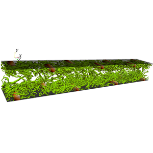
Figure 1. Schematic of a segment of channel’s configuration with asymmetric rough walls of staggered elements.
Figure 1 shows the schematic of the computational domain. The simulation is carried out in a three-dimensional Cartesian grid. The grid mesh increments in the three directions are  $\unicode[STIX]{x0394}x=\unicode[STIX]{x0394}y=\unicode[STIX]{x0394}z$. The cross-section of the channel has
  $120\times 128$ mesh points and the streamwise length of the channel extends up to 32 h. The simulations were carried out at Reynolds numbers of 2096 and 880 with periodic boundary conditions applied in the streamwise and spanwise directions. A no-slip boundary condition is implemented at the walls of the channel using a mid-grid bounce back scheme (Succi Reference Succi2001) which is of a second-order accuracy. It was first verified that the LBM simulation of a smooth wall laminar flow reproduced the Poiseuille distribution (not shown here). The channel was then roughened by mounting square bars transversally on the walls. The bars initially spanned the entire width of the channel. However, when it was found that this configuration did not generate turbulence, the bars were made to span only the half-width of the channel and mounted in a staggered fashion (see figure 1). The square bars height,
  $k$, is represented by 16 mesh points. The separation,
  $p$, between two consecutive aligned roughness elements is
  $p=18k$, while the distance between two consecutive staggered elements is
  $8k$. Table 1 summarizes the flow conditions.
Table 1. Channel flow conditions.

3 Results
Since it was found that no turbulence was generated when the bars spanned the entire width of the channel (see Anika et al. (Reference Anika, Djenidi and Tardu2018) for a discussion of this case), we do not present the results pertaining to this flow roughness configuration. The focus is only on the configuration with the bars spanning half the width of the channel.
3.1 Flow visualizations
‘Numerical’ flow visualizations are performed using the  $\unicode[STIX]{x1D706}_{2}$-method (Jeong & Hussain Reference Jeong and Hussain1995). The method is based on the eigenvalues of the symmetric
  $3\times 3$ tensor
 $$\begin{eqnarray}\unicode[STIX]{x1D614}_{ij}=\unicode[STIX]{x1D6F4}_{k}(S_{ik}S_{kj}+D_{ik}D_{kj}),\end{eqnarray}$$
 with  $k=1,2$ and 3 (along the
  $x$,
$x$,  $y$ and
  $z$ directions, respectively) and
 $$\begin{eqnarray}\displaystyle & \displaystyle S_{ij}=\frac{1}{2}\left({\displaystyle \frac{\unicode[STIX]{x2202}u_{i}}{\unicode[STIX]{x2202}x_{j}}}+{\displaystyle \frac{\unicode[STIX]{x2202}u_{j}}{\unicode[STIX]{x2202}x_{i}}}\right), & \displaystyle\end{eqnarray}$$
 $$\begin{eqnarray}\displaystyle & \displaystyle D_{ij}=\frac{1}{2}\left({\displaystyle \frac{\unicode[STIX]{x2202}u_{i}}{\unicode[STIX]{x2202}x_{j}}}-{\displaystyle \frac{\unicode[STIX]{x2202}u_{j}}{\unicode[STIX]{x2202}x_{i}}}\right) & \displaystyle\end{eqnarray}$$
 are the symmetric and antisymmetric components, respectively, of the velocity gradient tensor  $\unicode[STIX]{x1D735}\boldsymbol{u}$; note that in the rest of the text we use interchangeably the notation
  $u_{1}$,
  $u_{2}$,
  $u_{3}$ and
  $u$,
$u$,  $v$,
$v$,  $w$, respectively. The tensor
  $\unicode[STIX]{x1D614}_{ij}$ has three real eigenvalues:
  $\unicode[STIX]{x1D706}_{1},\unicode[STIX]{x1D706}_{2}$ and
  $\unicode[STIX]{x1D706}_{3}$. Jeong & Hussain (Reference Jeong and Hussain1995), argued that
  $\unicode[STIX]{x1D614}_{ij}$, can be used to determine the existence of a local pressure minimum associated with vortical motion and showed that a vortex core can be identified as any continuous region where two of the eigenvalues of
  $\unicode[STIX]{x1D614}_{ij}$ are negative. If the eigenvalues are sorted such that
  $\unicode[STIX]{x1D706}_{3}\leqslant \unicode[STIX]{x1D706}_{2}\leqslant \unicode[STIX]{x1D706}_{1}$, then any region for which
  $\unicode[STIX]{x1D706}_{2}\leqslant 0$ corresponds to a vortex core. This method allows following of the development of any vortical structures in the flow.

Figure 2. Flow visualization based on  $\unicode[STIX]{x1D706}_{2}$-contour
  $(\unicode[STIX]{x1D706}_{2}/\unicode[STIX]{x1D706}_{2,max}=-0.02)$ on staggered rough wall at: (a)
  $Re_{b}=2093$, (b)
  $Re_{b}=880$. The section of the channel shown here is
  $(8\leqslant x/h\leqslant 20)$.
Figure 2 shows a snapshot of  $\unicode[STIX]{x1D706}_{2}$ structures for both Reynolds numbers. Recall that no initial turbulent field or noise was used to trigger turbulence. The figure reveals coherent elongated structures across the channel, which appear to evolve considerably in a folding and stretching manner as they are transported with the mean flow. Note the significant more populated field for the highest Reynolds number, where the structures are much finer and shorter that in the case of the lower Reynolds number. These structures exhibit similar features to those present in a fully turbulent channel flow (either on a smooth or rough wall) indicating that this roughness configuration not only generates but also maintains turbulence once generated.
Anika et al. (Reference Anika, Djenidi and Tardu2018) showed that two pulsed jets shifted in a spanwise direction activate the bypass the transition mechanism through ejection of spanwise vorticity from the canopy (their figure 5) which is consistent with the ejection of vorticity above arrays of cubical obstacles (Leonardi & Castro Reference Leonardi and Castro2010). The passive bypass transition mechanism investigated here differs from that in Anika et al. (Reference Anika, Djenidi and Tardu2018) in many respects. In order to investigate the initial turbulence generation mechanism we carried out simulations in a non-periodic channel flow in the streamwise direction where the width was doubled. This allows us to follow any disturbance and assess its growth as it is entrained in a laminar regime before the flow becomes turbulent. This is not possible with a periodic condition in  $x$. Further, this approach is more realistic and more similar to experiments where the incoming flow at the inlet of the working section is in the laminar regime. Finally, the ratio
  $k/h$ was halved in comparison to the one used in the periodic channel flow.

Figure 3. Flow visualization at the entrance of the non-periodic channel flow ( $Re_{b}=2093$). Contours of the vorticity magnitude at several heights from the bottom wall,
  $y/k=0.5$ (a), 1 (b), 1.5 (c), 2, (d), 3 (e) and 4 (f). The three sections of the channel shown here cover the range
  $1\leqslant x/h\leqslant 19$. On each image, the flow is from left to right. The levels of the vorticity magnitude range from 0 (dark blue) to 0.03 (red).
Figure 3 shows a plane view of the magnitude of the instantaneous vorticity,  $\unicode[STIX]{x1D714}$, at several heights from the bottom wall:
  $y/k=0.5$, 1, 1.5, 2, 3 and 4 and for the distance
  $1\leqslant x/h\leqslant 19$. Starting at the plane
  $y/k=0.5$, that is below the bar height, we observe that, in the early stage of the flow (
 $1\leqslant x/h\leqslant 6$),
  $\unicode[STIX]{x1D714}$ is practically zero, except at the lateral ends of the roughness elements where a spanwise variation is seen. This variation increases while spreading laterally as the flow progresses along the channel. At the end of the last section (
 $18\leqslant x/h\leqslant 19$), the vorticity has spread over the whole span of the channel. This scenario is observed at all heights shown on the figure. Note, however, that, as
  $y/k$ increases, the flow remains longer in the pseudo laminar regime. This is because the disturbances originated at the roughness level are simply transported with the main flow. Figure 3(a,b) shows that each roughness element induces a disturbance in the spanwise direction at its ends. Also, one can discern patterns in figure 3(b–d) in the form of ‘pseudo-streaks’ (discussed in the next paragraph). To better illustrate these patterns, we report in figures 4(a) and 4(b) a single contour of the enstrophy (
 $\unicode[STIX]{x1D714}^{2}$) coloured by
  $\unicode[STIX]{x1D714}_{y}$, the vertical component of
  $\unicode[STIX]{x1D714}$. We can see the presence of pseudo-periodic longitudinal structures over the section of the channel shown, although the structures become less coherent in the last section. It seems that, at first, there are two flows in parallel, each delimited by the roughness extremities. This is clearly visible in the first section. In this section, the flow is in a pseudo-laminar regime, which explains the strong coherence of the longitudinal structures. In the second (or middle) section, new structures are generated at the roughness ends below the already established structures that are convected by the flow. In the last section, new structures are also formed at the roughness extremities, and they quickly interact with the existing ones, resulting in a multiplication of structures, as seen in figure 5 where we reproduced for convenience the last section of the three reported in figure 4. This figure shows well the interlacing and merging of the newly created and old coherent structures.

Figure 4. Flow visualization (non-periodic channel flow,  $Re_{b}=2093$): enstrophy contour coloured with the vertical component of the vorticity,
  $\unicode[STIX]{x1D714}_{y}$, for better visualization effect; the level of the
  $\unicode[STIX]{x1D714}_{y}$-contours range from
  $-0.002$ to 0.002. (a) Perspective view; (b) top view. Same range of
  $x/h$ as in figure 3. Flow is from left to right.

Figure 5. Flow visualization (non-periodic channel flow,  $Re_{b}=2093$): enstrophy contour coloured with the vertical component of the vorticity,
  $\unicode[STIX]{x1D714}_{y}$; same as in perspective view of figure 4 but for
  $13\leqslant x/h\leqslant 19$.
Elongated positive and negative  $\unicode[STIX]{x2202}u/\unicode[STIX]{x2202}z$ shear layers that are part of the wall-normal component of vorticity
  $\unicode[STIX]{x1D714}_{y}=\unicode[STIX]{x2202}u/\unicode[STIX]{x2202}z-\unicode[STIX]{x2202}w/\unicode[STIX]{x2202}x$ are established upon the channel entry (figure 6). They are set up between the staggered roughness elements and slightly oscillate in the streamwise direction before the formation of a fully developed turbulent spot at in the zone
  $C$ delimited by
  $14\leqslant x/h\leqslant 19$. In a fully developed smooth wall turbulent flow, thin wall regions of
  $\unicode[STIX]{x2202}u/\unicode[STIX]{x2202}z$ mark the spanwise ends of the high and low speed streaks induced by the quasi-streamwise vortices. This is not the case in the early stages of the bypass transition process in zone
  $A$, i.e.
  $0\leqslant x/h\leqslant 10$, wherein only a few quasi-streamwise vortices are triggered, as we will discuss later. The
  $\unicode[STIX]{x2202}u/\unicode[STIX]{x2202}z$ shear layers in the zone
  $A$ of figure 6 originate from the flow kinematics as a result of the spanwise asymmetry between the staggered roughness elements. The
  $-\unicode[STIX]{x2202}w/\unicode[STIX]{x2202}x$ component of
  $\unicode[STIX]{x1D714}_{y}$, in turn, plays a key active role in the early stages of the transition process initiated in region
  $A$. The spanwise velocity fluctuations are rapidly set up through the local pressure gradient
  $\unicode[STIX]{x2202}p/\unicode[STIX]{x2202}z$ and positive and negative
  $\unicode[STIX]{x2202}w/\unicode[STIX]{x2202}x$ layers appear near the tips of the roughness elements at the channel entrance zone (figure 7). The main production term of the streamwise vorticity transport equation is the tilting of the wall-normal vorticity, which reduces to
  $(-\unicode[STIX]{x2202}w/\unicode[STIX]{x2202}x)(\unicode[STIX]{x2202}(\overline{U}+u)/\unicode[STIX]{x2202}y)$ (Brooke & Hanratty Reference Brooke and Hanratty1993). There are intense
  $\unicode[STIX]{x2202}(\overline{U}+u)/\unicode[STIX]{x2202}y$ local shear zones near the tips and between the staggered roughness elements, as seen in figure 8. The accumulation of the streamwise vorticity and the strong discontinuity, induced by the tips of the roughness elements, constitute the necessary ingredients for the roll-up of the
  $\unicode[STIX]{x1D714}_{x}$ layers into quasi-streamwise vortices (Jiménez & Orlandi Reference Jiménez and Orlandi1993). It is clearly seen in figure 9 that the
  $\unicode[STIX]{x1D706}_{2}$ structures are sporadically triggered during the very beginning of the bypass transition process wherein
  $-\unicode[STIX]{x2202}w/\unicode[STIX]{x2202}x$-shear layers are concentrated. To better show the correspondence between the
  $-\unicode[STIX]{x2202}w/\unicode[STIX]{x2202}x$ layers and quasi-streamwise vortices, we zoom in on an arbitrary zone in the intermediate region
  $B$ in figures 7 and 9; we can observe such correspondences anywhere in the whole transition zone.

Figure 6. Contours of  $(\unicode[STIX]{x2202}u/\unicode[STIX]{x2202}z)\ast h/u_{b}$ shear layers at the entrance of the non-periodic channel flow (
 $Re_{b}=2093$). The colour code is as follows: pink,
  $-1.45$; blue, 1.45. The entry zone is divided into three parts; zone
  $A$ corresponds to the early transition zone and is delimited by
  $0\leqslant x/h\leqslant 10$; the zone
  $B$ is the intermediate transition region wherein the ensemble of transition ingredients take place (
 $10\leqslant x/h\leqslant 14$) and the turbulent spot appears in
  $C$, at
  $x/h\geqslant 14$. Same range of
  $x/h$ as in figure 3.

Figure 7. Contours of  $-(\unicode[STIX]{x2202}w/\unicode[STIX]{x2202}x)\ast h/u_{b}$ shear layers at the entrance of the non-periodic channel flow (
 $Re_{b}=2093$). The colour code is as follows: pink,
  $-1.45$; blue, 1.45. Same range of
  $x/h$ as in figure 6.
The wall-normal vorticity layers are the key elements that sustain the wall turbulence over a smooth wall, but also over the rough wall, and their suppression brings the flow back to a completely laminar state. The linearized  $\unicode[STIX]{x1D714}_{y}$ transport equation under these circumstances is
 $$\begin{eqnarray}\frac{\text{D}\unicode[STIX]{x1D714}_{y}}{\text{D}t}=-\frac{\unicode[STIX]{x2202}\overline{U}}{\unicode[STIX]{x2202}y}\frac{\unicode[STIX]{x2202}v}{\unicode[STIX]{x2202}z}+\unicode[STIX]{x1D708}\unicode[STIX]{x1D6FB}^{2}\unicode[STIX]{x1D714}_{y}\end{eqnarray}$$
 (Landahl Reference Landahl1980, Reference Landahl1990). This equation is subject to algebraic growth (Schmid & Henningson Reference Schmid and Henningson2012). Supposing that the normal velocity remains constant over time, the wave-type solutions of (3.4) lead indeed to a linear growth of  $\unicode[STIX]{x1D714}_{y}$ before the limiting effect of viscosity comes into the play. Figure 10 shows that the shear layers of
  $-\unicode[STIX]{x2202}v/\unicode[STIX]{x2202}z$ are already seen at the channel entry, and are also concentrated near the roughness tips. They are, however, less intense compared to
  $-\unicode[STIX]{x2202}w/\unicode[STIX]{x2202}x$ up to the start of the fully developed turbulent spot in the region
  $B$. The
  $-\unicode[STIX]{x2202}v/\unicode[STIX]{x2202}z$ patches grow and multiply in the latter and the algebraic streak growth mechanism (Schoppa & Hussain Reference Schoppa and Hussain2002) comes also into play. The early key triggering element of the quasi-streamwise coherent vortices generation is, however, the
  $-\unicode[STIX]{x2202}w/\unicode[STIX]{x2202}x$ shear layers. The roughness tips clearly play a role similar to that of vortex generators. As discussed before, there are no classical streaks at the very beginning of this process, which is different from the self-sustaining mechanism proposed by Waleffe (Reference Waleffe1997) and Hamilton, Kim & Waleffe (Reference Hamilton, Kim and Waleffe1995). However, once the bypass mechanism is achieved, and the quasi-streamwise vortices are generated, one has the set-up of near-wall streaks of the classical self-sustaining process similar to that over a smooth wall.

Figure 8. Contours of local  $(\unicode[STIX]{x2202}(\overline{U}+u)/\unicode[STIX]{x2202}y)\ast h/u_{b}$ shear layers at the entrance of the non-periodic channel flow. (
 $Re_{b}=2093$) The colour code is as follows: pink, 6.78; blue,
  $-6.78$. Same range of
  $x/h$ as in figure 6.

Figure 9. Contours of  $\unicode[STIX]{x1D706}_{2}/\unicode[STIX]{x1D706}_{2,min}=0.0035$ at the entrance of the non-periodic channel flow (
 $Re_{b}=2093$). Same range of
  $x/h$ as in figure 6.

Figure 10. Contours of local  $(\unicode[STIX]{x2202}v/\unicode[STIX]{x2202}z)\ast h/u_{b}$ shear layers at the entrance of the non-periodic channel flow (
 $Re_{b}=2093$). The colour code is as follows: pink,
  $-1.45$; blue, 1.45. Same range of
  $x/h$ as in figure 6.
Finally, figure 11 shows  $\unicode[STIX]{x1D706}_{2}/\unicode[STIX]{x1D706}_{2,max}=-0.02$ at an early stage of the periodic channel flow simulations with
  $k/h=0.27$. As for the case
  $k/h=0.13$ and the non-periodic channel flow simulation, structures are generated at the edges of the roughness elements, indicating that the turbulence generation mechanism is similar to that discussed above. However, due to the periodic nature of the simulation, the transition is faster.

Figure 11. Contours of  $\unicode[STIX]{x1D706}_{2}/\unicode[STIX]{x1D706}_{2,max}=-0.02$ at the entrance of the periodic rough wall channel (
 $Re_{b}=2093$) for
  $k/h=0.27$.
We complete this flow visualization section with images of the time averaged flow field. Due to the relatively small number of instantaneous flow fields (approximately 50), we followed the procedure used by Krogstad et al. (Reference Krogstad, Andersson, Bakken and Ashrafian2005) to increase the number of statistically independent samples and compute the time average. We used only the last section of the non-periodic channel ( $24\leqslant x/h\leqslant 32$) where the flow was almost fully developed, and exploited the streamwise periodicity of the average flow field: statistical equivalence between two points
  $(x,y,z)$ and
  $(x+nq,y,z)$, where
  $q$ is the pitch (between two consecutive aligned bars) and
  $n$ an integer, and with respect to its vertical anti-symmetry about the channel middle plane.

Figure 12. Time-averaged flow field in the non-periodic rough wall channel. (a) Contours of  $\overline{U}$ (ranging from 0 to
  $\overline{U}_{c}$;
  $c$ stands for centreline) in a vertical plane and a horizontal plane just above the roughness base plane; also shown are streamlines behind a roughness element. (b) Top view of the recirculatory motion. (c) Top view of contours of
  $\overline{W}$ (ranging from
  $-0.3\overline{U}_{c}$ to
  $0.3\overline{U}_{c}$) in an horizontal plane at
  $y/k=0.5$. The flow is from left to right. The last section of the non-periodic channel (
 $24\leqslant x/h\leqslant 32$) was used to carry out the averaging process.
Figure 12 shows that a recirculatory motion takes place behind the roughness elements which extends over a distance of approximately  $k$. As expected, this recirculation shows variations along the roughness element, although it is symmetric about the roughness mid-cross-section. The converging behaviour of the streamlines indicates the presence of a non-negligible mean spanwise velocity component
  $\overline{W}$ at the edges of the roughness elements, as seen in the figure. The velocity
  $\overline{U}$ exhibits a spanwise variation, which is better seen in figure 13 where contours of
  $\overline{U}$ at various horizontal planes are shown. The spanwise variation gradually dissipates as the distance to the wall increases. However, even at the last plane, which is at the half-height of the channel,
  $\overline{U}$ exhibits traces of the spanwise variation induced by the roughness. This lasting effect is certainly due to the value of the ratio
  $k/h$ which is approximately 0.13. One can expect, however, that the spanwise variation will eventually vanish as the computation domain is extended along the axis of the channel, so completely fully developed conditions are established.

Figure 13. Time-averaged flow field in the non-periodic rough wall channel. Contours of  $\overline{U}$ (ranging from 0 to
  $\overline{U}_{c}$) in horizontal planes at
  $y/k=0.125$, 1, 2, 4 and 8, from far left to far right; flow on each image is from left to right. The variation of
  $\overline{U}$ along a white line (seen in the left image for convenience) is 100 %, 91 %, 34 %, 20 % and 14 % for
  $y/k=0.125$, 1, 2, 4 and 8, respectively. The last section of the non-periodic channel (
 $24\leqslant x/h\leqslant 32$) was used to carry out the averaging process.

Figure 14. Time-averaged flow field in the periodic rough wall channel and  $k/h=0.27$. (a) Contours of
  $\overline{U}$ in a vertical plane and a horizontal plane just above the roughness base plane; also shown are streamlines behind a roughness element. (b) Top view of the recirculatory motion. (c) Top view of contours of
  $\overline{W}$ in an horizontal plane at
  $y/k=0.5$. The flow is from left to right. The ranges of the
  $\overline{U}$- and
  $\overline{W}$-contours are the same as in figure 12.

Figure 15. Time-averaged flow field in the periodic rough wall channel and  $k/h=0.27$. Contours of
  $\overline{U}$ (ranging from 0 to
  $\overline{U}_{c}$) in horizontal planes at
  $y/k=0.125$, 1, 2, 3 and 3.71 from far left to far right; flow on each image is from left to right. The ranges of the
  $\overline{U}$-contours are the same as in figure 12.
In order to demonstrate that the spanwise variation is indeed due to an insufficiently long channel, a similar averaging procedure was applied to the periodic channel with the larger roughness elements  $k/h=0.27$. The results are shown in figures 14 and 15. While the present roughness exhibits an obstacle-like behaviour, as reflected in the large recirculation behind the roughness elements, the spanwise variation is practically negligible for
  $y/k\geqslant 2.5$. Not surprisingly, the recirculation observed behind these staggered roughness elements differs from that behind transverse bars spanning the width of the channel. In this latter case the recirculation consists of a vortical motion with its axis aligned in the spanwise direction (as can be seen in, for example, figure 2 of Leonardi et al. (Reference Leonardi, Orlandi, Smalley, Djenidi and Antonia2003)), namely a spanwise vorticity
  $\unicode[STIX]{x1D6FA}_{z}$. The present recirculation is more complicated, as revealed by figures 12 and 14, and is primarily made of
  $\unicode[STIX]{x1D6FA}_{z}$ and
  $\unicode[STIX]{x1D6FA}_{y}$, the vertical vorticity components. The former dominates the centre of the bar, while the latter dominates toward the edges of the bar. Further, the aspect ratio
  $l_{b}/k$ (
 $l_{b}$ is the bar length in the
  $z$ direction) is likely to play a role in the size and features of the recirculation region;
  $l_{b}/k=15.6$ in figure 12, while
  $l_{b}/k=4$ in figure 14. Note the larger (and certainly with a stronger intensity in
  $\unicode[STIX]{x1D6FA}_{y}$) lateral motion at the sides of the bar when
  $l_{b}/k=4$.
In the next section we attempt to quantify the turbulent flow in order to ascertain whether it is similar to that of a fully developed turbulent channel flow, as reported in the literature. It the following we used a time-double space (along  $x$ and
  $z$) averaging procedure on the periodic channel flow simulation to ensure proper convergence of the statistics. Although this averaging hides any spanwise variations, particularly near the roughness elements, it is appropriate when the focus of the analysis is on the global effect of the roughness on the flow, as it is in this study.
3.2 Mean velocity
The distributions of the wall-unit-normalized mean velocity ( $U^{+}=\overline{U}/u_{\unicode[STIX]{x1D70F}}$) for both cases of
  $Re_{b}$ with the staggered roughness elements are reported in a semi-log representation in figure 16 as a function of
  $y^{+}=yu_{\unicode[STIX]{x1D70F}}/\unicode[STIX]{x1D708}$; the friction velocity,
  $u_{\unicode[STIX]{x1D70F}}$, is calculated via the pressure gradient as follows:
 $$\begin{eqnarray}u_{\unicode[STIX]{x1D70F}}=\sqrt{{\displaystyle \frac{h(\text{d}\overline{p}/\text{d}x)}{\unicode[STIX]{x1D70C}}}},\end{eqnarray}$$
 where  $\unicode[STIX]{x1D70C}$ is the density of fluid, and
  $p$ the pressure; the overbar represents time and space averaging along the
  $x$ and
  $z$ directions. We also show in the figure the distributions for our smooth wall and rough walls with the bars spanning the entire width of the channel. Reported too, for comparison, are the fully developed smooth wall turbulent channel flow of Moser, Kim & Mansour (Reference Moser, Kim and Mansour1999), and the rough wall turbulent channel flows of Krogstad et al. (Reference Krogstad, Andersson, Bakken and Ashrafian2005) and Leonardi et al. (Reference Leonardi, Orlandi, Smalley, Djenidi and Antonia2003); the roughness geometry used in the two latter studies are 2-D transverse bars spanning the entire channel flow (only one wall is rough in the study of Leonardi et al. (Reference Leonardi, Orlandi, Smalley, Djenidi and Antonia2003)). Only the distributions over half the heights of the channels are shown and, for simplicity, the origin of the profiles is taken at the base of the roughness elements. It should be recalled that the profile of Krogstad et al. (Reference Krogstad, Andersson, Bakken and Ashrafian2005) represents a time-averaged mean velocity profile measured above a roughness element, while the profiles of Leonardi et al. (Reference Leonardi, Orlandi, Smalley, Djenidi and Antonia2003) represent, as for the present profiles, space and time-averaged mean velocity distributions.

Figure 16. Mean velocity profiles normalized by  $u_{\unicode[STIX]{x1D70F}}$. Smooth wall,
  $Re_{b}=999$: – – – –, blue; transverse rough wall,
  $Re_{b}=1000$: –●–; staggered rough wall,
  $Re_{b}=880$: ——, blue and
  $Re_{b}=2093$: ——, black. DNS smooth wall,
  $Re_{h}=10\,700$:
  $\cdots \cdots$ (Moser et al. Reference Moser, Kim and Mansour1999). Rough wall,
  $Re_{b}=4200$,
  $h/k=0.035$,
  $p/k=8$: – – – –, black (Krogstad et al. Reference Krogstad, Andersson, Bakken and Ashrafian2005);
  $Re_{b}=4200$,
  $k/h=0.2$,
  $p/k=19$: –●– – – and
  $p/k=8$: –▵– (Leonardi et al. Reference Leonardi, Orlandi, Smalley, Djenidi and Antonia2003). The straight thin solid lines represent the log law. Inset: comparison between time- and space-averaged distribution and the ‘pseudo’ time-averaged ones for
  $Re_{b}=2093$;
  $z_{1}$ and
  $z_{2}$ mark the spanwise locations of the ‘pseudo’ time-averaged profiles.
When the channel walls are smooth for the present simulations, the flow remains, as expected, two-dimensional and laminar at both Reynolds numbers. The flow remains also two-dimensional and laminar when the roughness elements spanning the entire width of the channel are mounted on the walls, although steady state recirculatory motions sit in the spaces between the roughness elements. In this latter case, the friction velocity is increased, as reflected by the downward shift of the velocity profile when compared to the smooth wall case. This indicates a drag increase which stems from an increase of the wall velocity gradient at the top the roughness elements, even though the viscous drag is slightly negative between the roughness elements due to the recirculatory motion. The situation is significantly different when the bars span only half the width of the channel. While the profiles exhibit an expected downward shift, associated with an increase of the friction velocity, the shift is relatively large. Indeed, although the Reynolds numbers of the present simulations are smaller than those of Krogstad et al. (Reference Krogstad, Andersson, Bakken and Ashrafian2005) and Leonardi et al. (Reference Leonardi, Orlandi, Smalley, Djenidi and Antonia2003), the downward shift is of similar magnitude to that exhibited by the profiles of these latter studies. It should be mentioned that  $Re_{b}$, which was approximately 1000 for both the smooth wall and the wall with non-staggered roughness, increased to approximately 2000 after mounting the staggered roughness on the walls while keeping all other parameters fixed. To achieve the lower Reynolds number in the staggered roughened channel flow, the velocity had to be reduced, implying that
  $Re_{b}$ for the corresponding smooth wall channel flow would be even smaller than 1000, well within the laminar regime.
A remarkable feature exhibited by the staggered rough wall velocity profiles is that they are similar in shape to those observed in a fully developed turbulent channel flow. In particular, they reveal an apparent logarithmic region, albeit over a rather shorter range of  $y^{+}$ than their DNS counterparts, certainly due to the lower value of
  $Re_{b}$ achieved in the present case. The present distributions show a somewhat different behaviour than those of Leonardi et al. (Reference Leonardi, Orlandi, Smalley, Djenidi and Antonia2003) as the wall is approached. Notice the inflection point at
  $y^{+}\simeq 15$ and 40 in the present distribution for
  $Re_{b}=880$ and 2093, respectively; both locations correspond to
  $y=0.375k$, well below the roughness height. This difference is not surprising considering the actual difference in the roughness arrangement between the two simulations. Certainly, the spanwise inhomogeneity of the time-averaged velocity profile near the present roughness as seen in figure 13 accounts for the difference with Leonardi et al. (Reference Leonardi, Orlandi, Smalley, Djenidi and Antonia2003). The spanwise inhomogeneity is well captured in the ‘pseudo’ time-average distributions computed at the same
  $x$ position, but two different spanwise locations, one above and middle of the bar, the other shifted off the bar. These distributions are reported in the inset of figure 16 where a linear–linear scale is used; also reported for comparison only in the inset is the time- and spaced-averaged distribution of the main figure. As anticipated from the flow visualization in figure 15, the spanwise variation reduces as
  $y$ increases; the variation is 13 %, 3 % and 0 at
  $y/k=2$,
  $y/k=3$ and
  $y/k=3.71$ (the channel centreline), respectively.
A final interesting observation concerning the velocity profiles over the staggered roughness elements relates to the fact that the downward shift magnitude quantified by  $\unicode[STIX]{x0394}U^{+}=U_{r}^{+}-U_{s}^{+}$ (where
  $U_{r}$ and
  $U_{s}$ are the rough wall and smooth wall velocities measured within or beyond the log region of the velocity profiles) is larger for the staggered rough wall case than that of Krogstad et al. (Reference Krogstad, Andersson, Bakken and Ashrafian2005), even though
  $Re_{b}$ of the former cases is four and two times, respectively, smaller than that of the latter study. The relatively strong downward shift in our data in comparison to that of Krogstad et al. (Reference Krogstad, Andersson, Bakken and Ashrafian2005) may suggest that 3-D wall geometries lead to disturbances larger than 2-D wall geometries. However, the 2-D wall geometry of Leonardi et al. (Reference Leonardi, Orlandi, Smalley, Djenidi and Antonia2003) exhibits a larger downward shift for the same ratio
  $p/k=8$. It is likely that the effect of the ratio
  $h/k$ affects the magnitude of the downward shift. The present ratio is approximately 0.26, while that of Krogstad et al. (Reference Krogstad, Andersson, Bakken and Ashrafian2005) is approximately 0.03. This effect of
  $h/k$ is also reflected in the data of Leonardi et al. (Reference Leonardi, Orlandi, Smalley, Djenidi and Antonia2003) reported here and for which
  $h/k=0.2$. The large value of the present downward shift reflects the large value of the drag, likely to be associated with the relatively large value of
  $k/h$. Indeed, the mean velocity profiles show that
  $\unicode[STIX]{x2202}U^{+}/\unicode[STIX]{x2202}y^{+}$ at the wall is practically zero (this is very evident when a linear–linear plot is used) indicating that the viscous drag is practically negligible. The dominance of the form drag indicates that the density, the shape and layout of the 2-D and 3-D roughnesses certainly play roles in the effect on the roughness on the flow. For example, the effect of the density was well demonstrated by Leonardi & Castro (Reference Leonardi and Castro2010). Also, Bakken et al. (Reference Bakken, Krogstad, Ashrafian and Andersson2005) reported that the 2-D rough wall produced a larger downward shift in the mean velocity profile than a wire-meshed rough wall.

Figure 17. Present distributions of  $\overline{u_{i}^{\prime +2}}$ (
 $i=1,2$ and 3) for
  $Re_{b}=880$ (lines with solid circles),
  $Re_{b}=2093$ (solid lines). Solid lines: present simulations. Dashed, dotted and dash-dotted lines: DNS smooth wall (Moser et al. Reference Moser, Kim and Mansour1999). Blue,
  $u_{1}^{\prime +2}$; red,
  $u_{2}^{\prime +2}$; black,
  $u_{3}^{\prime +2}$. The origin
  $y/h=0$ for the rough wall data is the base wall and the location
  $y/k$ represents the location of the roughness crest plane.
3.3 Reynolds stresses
Figure 17 shows the distributions  $\overline{u_{i}^{+2}}$ (
 $i=1$, 2 and 3) for
  $Re_{b}=880$ and
  $Re_{b}=2093$. Due to the symmetry of the distributions across the channel height, only the part of the distributions across the lower half-height is reported; the origin
  $y/h=0$ is taken at the base of the roughness elements. Also reported for comparison are the DNS distributions for the smooth wall channel flow of Moser et al. (Reference Moser, Kim and Mansour1999). Near the wall, the streamwise Reynolds stress
  $\overline{u_{1}^{+2}}$ is the largest component, while the wall-normal Reynolds stress
  $\overline{u_{2}^{+2}}$ is the smallest. Notice that the maximum for each distribution is reached at different heights. These maxima are reached at
  $y/h\simeq 0.07$, 0.19 and 0.33 for
  $\overline{u_{3}^{+2}}$,
  $\overline{u_{1}^{+2}}$ and
  $\overline{u_{2}^{+2}}$, respectively. Of interest,
  $\overline{u_{3}^{+2}}$ exhibits a clear hump at approximately the same height where
  $\overline{u_{2}^{+2}}$ is maximum. We also observe that while the magnitude of the Reynolds stresses decreases as
  $Re_{b}$ decreases, the maximum of
  $\overline{u_{3}^{+2}}$ appears to present the stronger reduction, which is indicative of a reduced spanwise activity within the roughness vicinity;
  $\overline{u_{1}^{+2}}$ shows the lowest reduction. The behaviour of
  $\overline{u_{3}^{+2}}$ below the location
  $y/k=1$ departs in a major manner from that of
  $\overline{u_{1}^{+2}}$ and
  $\overline{u_{2}^{+2}}$. Indeed, both
  $\overline{u_{1}^{+2}}$ and
  $\overline{u_{2}^{+2}}$ decrease monotonically from their maximum to reach zero at the wall while,
  $\overline{u_{3}^{+2}}$ decreases slightly after a local maximum at
  $y/h=0.33$ then increases, reaches a maximum and finally decreases. The near-wall behaviour of
  $\overline{u_{3}^{+2}}$ is likely to reflect a strong spanwise activity caused by the present roughness elements, as anticipated from the flow visualizations. No such behaviour is observed in the case of 2-D transverse bars spanning the entire width of the channel (Ikeda & Durbin Reference Ikeda and Durbin2007; Burattini et al. Reference Burattini, Leonardi, Orlandi and Antonia2008).
The comparison between the smooth wall data and the present ones shows differences in behaviour and magnitude. For example, the maximum of  $\overline{u_{1}^{+2}}$ is significantly reduced on the rough wall. This is also observed in the data of Ikeda & Durbin (Reference Ikeda and Durbin2007), Burattini et al. (Reference Burattini, Leonardi, Orlandi and Antonia2008) and Krogstad et al. (Reference Krogstad, Andersson, Bakken and Ashrafian2005). Worthy to note are the levels of
  $\overline{u_{3}^{+2}}$ in the region
  $y/k\leqslant 1$ and that of
  $\overline{u_{2}^{+2}}$ above the plane
  $y/k=1$ in comparison to the smooth wall data. These levels indicate that the increase in
  $\overline{u_{3}^{+2}}$ is related to the activity taking place at the sides of roughness while the increase of
  $\overline{u_{2}^{+2}}$ is associated with an upward deflection of the flow caused by the roughness. However, one can expect that the magnitude of these increases to be controlled by the ratios
  $k/h$ and
  $p/k$.

Figure 18. Distributions of  $\overline{u^{\prime +2}}$,
  $\overline{v^{\prime +2}}$ and
  $\overline{w^{\prime +2}}$ for
  $Re_{b}=2093$ (solid lines). DNS rough wall data of Krogstad et al. (Reference Krogstad, Andersson, Bakken and Ashrafian2005): dashed lines. Blue,
  $u_{1}^{\prime +2}$; red,
  $u_{2}^{\prime +2}$; black,
  $u_{3}^{\prime +2}$. The origin
  $y/h=0$ for the rough wall data is the base wall and the location
  $y/k=1$ represents the location of the roughness crest plane for the present simulation.
Similar observations can be made when we compare the present Reynolds stress distributions with those of Krogstad et al. (Reference Krogstad, Andersson, Bakken and Ashrafian2005). For example, we report in figure 18 the distributions for  $Re_{b}=2093$ and those of Krogstad et al. (Reference Krogstad, Andersson, Bakken and Ashrafian2005). Recalling that the latter distributions are only time averaged and measured above a roughness element, the values of
  $\overline{u^{\prime +2}}$,
  $\overline{v^{\prime +2}}$ and
  $\overline{w^{\prime +2}}$ for these distributions must be zero at
  $y/h=0.034$, the location of the roughness crest plane; caution must be taken in analysing the differences between the two simulations. While the present distributions show similarities with those of Krogstad et al. (Reference Krogstad, Andersson, Bakken and Ashrafian2005), there are noticeable differences. For example, the present distribution of
  $\overline{u^{\prime +2}}$ exhibits a larger maximum than that of Krogstad et al. (Reference Krogstad, Andersson, Bakken and Ashrafian2005). Also, in the present case
  $\overline{v^{\prime +2}}$ is larger than that of Krogstad et al. (Reference Krogstad, Andersson, Bakken and Ashrafian2005) for
  $y/k\geqslant 1$. Considering that
  $Re_{b}$ for Krogstad et al. (Reference Krogstad, Andersson, Bakken and Ashrafian2005) is more than twice the present one, these differences in magnitudes of
  $\overline{u^{\prime +2}}$ and
  $\overline{v^{\prime +2}}$ are certainly related to the difference in the ratio
  $k/h$ between the two simulations. The ratio
  $k/h$ for the present simulation is approximately 0.25 while it is approximately 0.034 for Krogstad et al. (Reference Krogstad, Andersson, Bakken and Ashrafian2005). Note, however, (as inferred from figure 17) that the magnitudes of the Reynolds stresses are smaller for the present simulation when
  $Re_{b}=880$ than those of Krogstad et al. (Reference Krogstad, Andersson, Bakken and Ashrafian2005), showing that at this Reynolds number the roughnesses are less effective than at the larger one for producing strong turbulence level. This is expected as the lower the Reynolds number, the stronger the damping effect of the viscosity.
A comment is warranted regarding the relatively large value of  $k$ for the present simulation. One may consider that the roughness is akin to an obstacle rather than a roughness. However, as seen above, the distributions of the mean velocity and the Reynolds stresses are similar to those observed in a rough wall channel flow. Perhaps the combination of using bars spanning only half of the width of the channel and the present spacing between the bars helps reduce the blockage effect and allows the flow to resemble that of a channel flow over a rough wall; hence, one can refer to these bars as roughness elements rather than obstacles. This resemblance to a fully developed channel flow is further illustrated by the Reynolds shear stress distributions
  $-\overline{u^{+}v^{+}}$ shown in figure 19. Such distributions should present a linear variation across the channel height for a fully developed channel flow, as illustrated by the distribution of Moser et al. (Reference Moser, Kim and Mansour1999) and Krogstad et al. (Reference Krogstad, Andersson, Bakken and Ashrafian2005) also reported in the figure. Such behaviour is well observed in the present distributions for both values of
  $Re_{b}$.
The data of figures 16, 18 and 19 suggest a fully developed turbulent channel flow. This is further supported by figure 20, showing the correlation coefficient  $\unicode[STIX]{x1D70C}_{uv}=-\overline{u^{+}v^{+}}/(u^{\prime }v^{\prime })$. Indeed, in the region
  $0.2\leqslant y/h\leqslant 0.6$,
  $\unicode[STIX]{x1D70C}_{uv}$ falls in the range 0.35–0.41, which is the range reported in the literature for fully developed turbulent channel flows and turbulent boundary layers. Also, the present
  $\unicode[STIX]{x1D70C}_{uv}$ exhibits the expected Reynolds number dependence:
  $\unicode[STIX]{x1D70C}_{uv}$ decreases as
  $Re_{\unicode[STIX]{x1D70F}}$ increases. Reported for comparison in the figure is the
  $\unicode[STIX]{x1D70C}_{uv}$-distribution of Krogstad et al. (Reference Krogstad, Andersson, Bakken and Ashrafian2005), whose values of
  $\unicode[STIX]{x1D70C}_{uv}$ in the region
  $0.2\leqslant y/h\leqslant 0.4$ exceed 0.4.

Figure 19. Distributions of  $-\overline{(u^{+}v^{+})}$. Symbols: present simulation,
  $Re_{b}=880$ (blue) and
  $Re_{b}=2093$ (red). Solid line: smooth wall (Moser et al. Reference Moser, Kim and Mansour1999). Dashed line: rough wall (Krogstad et al. Reference Krogstad, Andersson, Bakken and Ashrafian2005). The origin
  $y/h=0$ is taken at the roughness crest plane.

Figure 20. Correlation coefficient  $\unicode[STIX]{x1D70C}_{uv}=\overline{uv}/(u^{\prime }v^{\prime })$. Symbols same as figure 19. Line: rough wall (Krogstad et al. Reference Krogstad, Andersson, Bakken and Ashrafian2005). The origin
  $y/h=0$ is taken at the roughness crest plane.
3.4 Energy budget
The kinetic energy budget can be written as
 $$\begin{eqnarray}\frac{\text{D}k}{\text{D}t}=P+T+D+\unicode[STIX]{x1D6F1}-\overline{\unicode[STIX]{x1D716}},\end{eqnarray}$$
 where  $P=-\overline{uv}(\text{d}\overline{U}/\text{d}y)$ is the turbulence production,
  $T=-\unicode[STIX]{x2202}\overline{(vk)}/\unicode[STIX]{x2202}y$ is the turbulent diffusion,
  $D=\unicode[STIX]{x1D708}(\unicode[STIX]{x2202}^{2}k/\unicode[STIX]{x2202}y^{2})$ is the viscous diffusion,
  $\unicode[STIX]{x1D6F1}=-\unicode[STIX]{x2202}\overline{(vp/\unicode[STIX]{x1D70C})}/\unicode[STIX]{x2202}y$ is the ‘pressure diffusion’ and
  $\overline{\unicode[STIX]{x1D716}}=2\unicode[STIX]{x1D708}\overline{(\unicode[STIX]{x2202}u_{i}/\unicode[STIX]{x2202}x_{k})(\unicode[STIX]{x2202}u_{j}/\unicode[STIX]{x2202}x_{k})}$ is the dissipation. In this equation, the terms have been averaged in time and in both the streamwise and spanwise directions. Also, the dispersive effects, which arise due to the non-uniform distribution of mean quantities in the streamwise and spanwise directions, are not accounted for in (3.6). These effects are mostly important in the vicinity of the roughness elements (Leonardi et al. Reference Leonardi, Orlandi, Djenidi and Antonia2006) where the streamwise non-uniformity is important. Note that, for the present rough wall, there is a further non-uniformity in the spanwise direction in the vicinity of the roughness. Thus, in the following discussion, it should be kept in mind that the present energy budgets do not account for any local streamwise and spanwise variations in the mean turbulent kinetic energy. To account for these variations requires time averaging only, which would necessitate running the simulations over an impractical extremely long time to ensure convergence of the various terms in (3.6). Nevertheless, the use of the time–space-average procedure allows comparisons with the time–space-averaged energy budget of Ikeda & Durbin (Reference Ikeda and Durbin2007) and Leonardi et al. (Reference Leonardi, Orlandi, Djenidi and Antonia2006).

Figure 21. Turbulent kinetic energy budget, normalized by  $u_{\unicode[STIX]{x1D70F}}^{3}/h$, as a function of
  $y/h$;
  $Re_{b}=880$ (a) and 2093 (b). Solid line in the top figure: balance of the budget terms in (3.6).

Figure 22. Reproduction of the turbulent kinetic energy budget near the rough wall of Ikeda & Durbin (Reference Ikeda and Durbin2007). The budget terms are normalized by  $u_{\unicode[STIX]{x1D70F}}^{4}/\unicode[STIX]{x1D708}$; see Ikeda & Durbin (Reference Ikeda and Durbin2007) for details on the various symbols.

Figure 23. Turbulent kinetic energy budget for  $Re_{b}=2093$, normalized by
  $u_{\unicode[STIX]{x1D70F}}^{4}/\unicode[STIX]{x1D708}$, as function of
  $y^{+}=yu_{\unicode[STIX]{x1D70F}}/\unicode[STIX]{x1D708}$ in the vicinity of the lower wall;
  $y=0$ represents the top plane of the roughness. Lines with symbols: present simulation (same as in figure 21); symbols only: simulation of Leonardi et al. (Reference Leonardi, Orlandi, Djenidi and Antonia2006),
  $k/h=0.1$,
  $p/k=7$ and
  $Re_{b}=7000$. Inset: same as main figure but plotted as function of
  $y/k$.
Figure 21 shows the distributions of each term in (3.6), except the advection term (left side of (3.6)) which is nil, for  $Re_{b}=880$ and 2093. The energy budgets for the two Reynolds numbers, present similar features. Both
  $P$ and
  $\overline{\unicode[STIX]{x1D716}}$ are maximum near the roughness crest plane and decrease as the distance to the wall increases. In the central region of the channel
  $P$ becomes negligible and
  $\overline{\unicode[STIX]{x1D716}}$ is balanced by the turbulent diffusion,
  $T$, which too exhibits a maximum near the roughness elements. Note that,
  $\overline{\unicode[STIX]{x1D716}}=T$ at
  $y/h=1$ (the channel centreline) as in a smooth channel flow (Hoyas & Jiménez Reference Hoyas and Jiménez2006) and as it should be. Also near the roughness,
  $\unicode[STIX]{x1D6F1}$ increases significantly while it is practically zero in the central region of the channel. The viscous diffusion,
  $D$, is negligible across the channel, except near the roughness. In the region below the roughness crest, the balance changes. At the base (
 $y=0$),
  $\overline{\unicode[STIX]{x1D716}}$ is, as expected, practically balanced by
  $D$. Notice that, just below the roughness crest,
  $\unicode[STIX]{x1D6F1}$ has changed sign and reached a minimum. As the bottom wall is approached it reverses sign again, reaches a maximum then drops;
  $T$ first drops practically to zero, below the roughness crest, before reaching a maximum near the base and drops again to zero at the base. Figure 21 shows clearly that the flow around the roughness is dynamically controlled by the roughness. Figure 21(a) shows also the balance of the terms in (3.6). This balance represents the contribution from the dispersive effects. These are large in the vicinity of the roughness and dissipate quickly as the distance to the wall increases above the roughness elements. Similar results are observed for
  $Re_{b}=2093$.
The present budgets are remarkably similar to that of Ikeda & Durbin (Reference Ikeda and Durbin2007) obtained in a turbulent rough wall channel flow with transverse bar  $k/h=0.11$ and
  $p=9$ spanning the entire width of the channel (figure 22). The similarity between the present budgets and that of Ikeda & Durbin (Reference Ikeda and Durbin2007) strongly suggests that the present turbulent flow shares the same characteristics as those of fully developed turbulent channel flow over a 2-D rough wall. Notice thought that the largest difference between budgets in the
  $\unicode[STIX]{x1D6F1}$-term. The present one is much larger than that of Ikeda & Durbin (Reference Ikeda and Durbin2007).
We report in figure 23 the same  $Re_{b}$-distributions as in figure 21, but only in the region near the roughness crest and compare them with the DNS results of Leonardi et al. (Reference Leonardi, Orlandi, Djenidi and Antonia2006). These authors carried out a direct numerical simulation of a rough wall turbulent channel flow at
  $Re_{b}=7000$. The roughness consisted of square transverse bars mounted on one wall of the channel only and spanning the entire width of the channel, with
  $k/h=0.1$; several different spacings
  $w$ between the bars were investigated. Despite the differences in the Reynolds number, the roughness geometry and, more importantly, the values of
  $k/h$ between the simulation configurations, there is an acceptable correspondence between the results in the region
  $50<y^{+}<100$, where there is an approximate equilibrium between the production and the dissipation; this is well illustrated in the inset of figure 23, which shows the same data as the main figure but as a function of
  $y/k$. It should be recalled that the equilibrium zone
  $P=\overline{\unicode[STIX]{x1D716}}$ extends from
  $y^{+}=30$ to
  $y/h=0.6$ in smooth turbulent channel flows and it is exactly reached only at infinite Reynolds numbers. Further, this balance between
  $P=\overline{\unicode[STIX]{x1D716}}$ leads to the logarithmic velocity distribution (Tardu Reference Tardu2013). This appears to be the case here too, as suggested by the mean velocity profile (figure 16) where a nascent logarithmic region is visible. Large differences are, however, observed near the top plane of the roughness in the present configuration compared to Leonardi et al. (Reference Leonardi, Orlandi, Djenidi and Antonia2006). The production
  $P^{+}$ at
  $y^{+}=0$ (
 $y=0$ is taken the roughness crest) is for instance six times smaller here. There are several reasons for these differences. Perhaps the major one relates to the dispersive effects. As mentioned earlier, the non-homogeneity in the spanwise direction is likely to result in a more important dispersive effect than that of Leonardi et al. (Reference Leonardi, Orlandi, Djenidi and Antonia2006). Consequently, the pressure term peaks at around
  $y^{+}=18$ and relaxes slowly after. Note that the
  $\unicode[STIX]{x1D6F1}$-term contribution of Leonardi et al. (Reference Leonardi, Orlandi, Djenidi and Antonia2006) is larger than that of Ikeda & Durbin (Reference Ikeda and Durbin2007). Further, the roughness height ratio
  $k/h$ is three times larger in this investigation than in Leonardi et al. (Reference Leonardi, Orlandi, Djenidi and Antonia2006). One can thus expect that the combination of the spanwise inhomogeneity and larger ratio
  $k/h$ leads to some differences in the energy budget around the roughness region. The maximum production is
  $P^{+}=0.25$ over a smooth wall. It decreases to 0.08 in Leonardi et al. (Reference Leonardi, Orlandi, Djenidi and Antonia2006) and to 0.05 in the case
  $k^{+}=100$ for Ikeda & Durbin (Reference Ikeda and Durbin2007), which is close to the value we have here but where
  $k/h=0.12$ is three times smaller. The roughness parameters that play a critical role in the weakening of production near the top plane are not clearly identified in the literature, but large
  $k/h$ values lead to a sluggish
  $P^{+}$.
3.5 Velocity spectra

Figure 24. Kolmogorov-normalized velocity spectra at the channel centreline for  $Re_{\unicode[STIX]{x1D706}}\approx 63$ (
 $Re_{b}=2093$) and
  $Re_{\unicode[STIX]{x1D706}}\approx 32$ (
 $Re_{b}=880$). The symbols correspond to the velocity spectrum measured in a rough wall turbulent boundary layer. The asterisk represents Kolmogorov normalization, using either the isotropic expression,
  $\unicode[STIX]{x1D716}_{iso}$, or the actual one,
  $\unicode[STIX]{x1D716}_{actual}$, for calculating
  $\overline{\unicode[STIX]{x1D716}}$.
We have seen above that the addition of bars in a staggered manner in a laminar channel flow led to a fully developed turbulent channel flow even though  $Re_{b}$ is well below the critical Reynolds number. It is then of interest to ascertain how the energy is distributed among the scales of motion or, in other words, ascertain what is the velocity spectrum exhibited by this turbulence. Figure 24 shows the longitudinal velocity spectrum at the channel centreline for both
  $Re_{b}$. The spectra are Kolmogorov normalized (the asterisk represents Kolmogorov normalization). To obtain the Kolmogorov length scale,
  $\unicode[STIX]{x1D702}=(\unicode[STIX]{x1D708}^{3}/\overline{\unicode[STIX]{x1D716}})^{1/4}$, and velocity scale,
  $\unicode[STIX]{x1D702}=(\unicode[STIX]{x1D708}\overline{\unicode[STIX]{x1D716}})^{1/4}$, we calculate
  $\overline{\unicode[STIX]{x1D716}}$, the mean turbulent kinetic energy dissipation, using its isotropic surrogate, i.e.
  $\overline{\unicode[STIX]{x1D716}}_{iso}=15\unicode[STIX]{x1D708}\overline{(\text{d}u/\text{d}x)^{2}}$ and its actual expression. Note that a time series of
  $u$ was used to compute the spectra and
  $\overline{\unicode[STIX]{x1D716}}$; the Taylor hypothesis to convert the time derivative into a spatial derivative was also used. Also reported in the figure for comparison is the Kolmogorov-normalized velocity spectrum measured in a rough wall turbulent boundary layer at
  $y/\unicode[STIX]{x1D6FF}=0.4$ where the Taylor microscale Reynolds number
  $Re_{\unicode[STIX]{x1D706}}$ is equal to approximately 133;
  $\overline{\unicode[STIX]{x1D716}}_{iso}$ was used to normalize the spectrum (details of the measurements can be found in Kamruzzaman et al. (Reference Kamruzzaman, Djenidi, Antonia and Talluru2015)).
Firstly, we observe that the present spectra normalized using  $\overline{\unicode[STIX]{x1D716}}_{iso}$, collapse well with the boundary layer spectrum in the range
  $0.03\leqslant k^{\ast }\leqslant 0.9$. While the use of
  $\overline{\unicode[STIX]{x1D716}}_{iso}$ for normalization purposes may not be strictly correct for wall shear flows, it is nevertheless appropriate to compare the spectra using the same normalization parameter,
  $\overline{\unicode[STIX]{x1D716}}_{iso}$ here. The collapse of the spectra in the high range of
  $k^{\ast }$ is consistent with the results of Antonia, Djenidi & Danaila (Reference Antonia, Djenidi and Danaila2014), who showed that the Kolmogorov-normalized spectra obtained in various turbulent flows collapse very well in the dissipative region for
  $Re_{\unicode[STIX]{x1D706}}$ as low as 30, thus validating Kolmogorov 1st similarity hypothesis (Kolmogorov Reference Kolmogorov1941), although Djenidi et al. (Reference Djenidi, Tardu, Antonia and Danaila2014) showed that this similarity breaks down for
  $Re_{\unicode[STIX]{x1D706}}\leqslant 20$.
Secondly, for the present simulation, we see that spectra normalized using  $\overline{\unicode[STIX]{x1D716}}_{iso}$ collapse relatively well with the ones normalized using
  $\overline{\unicode[STIX]{x1D716}}_{actual}$, the actual expression of
  $\overline{\unicode[STIX]{x1D716}}$, albeit the collapse is less remarkable for
  $Re_{b}=880$ than
  $Re_{b}=2083$. This result suggests that the local isotropy is better satisfied for the higher Reynolds number. It is likely that the inhomogeneity affects more significantly the small scales at the lower Reynolds number than the higher one.
Finally, the results of figure 24, which shows a continuous distribution of energy among all scales of motion, confirms that the turbulence characteristics generated in this relatively low Reynolds number channel flow are similar to those of a fully developed turbulence albeit at a low  $Re_{\unicode[STIX]{x1D706}}$.
4 Concluding remarks
A direct numerical simulation based on the lattice Boltzmann method is carried out in a rough wall channel flow initially in a laminar regime. Two (bulk velocity) Reynolds numbers are used,  $Re_{b}=880$ and 2093. Although not shown here, it is found that, when the roughness elements consisted of transverse bars of square cross-section spanning the entire width of the channel with
  $p=8k$ and
  $h/k=3.71$, the flow remains laminar, with a steady low intensity vortical motion taking place between the roughness elements. Only when the roughness elements spanned half the channel width (in a staggered fashion) is turbulence generated and maintained for both cases of
  $Re_{b}$. The turbulent flow in the channel exhibits similar characteristics to a fully developed turbulent channel flow on a rough wall. For example, the roughness function, measured as a downward shift of the mean velocity profile in comparison to that of a smooth wall, is comparable to that observed in fully rough turbulent channel flows at much higher Reynolds numbers. Even the turbulent kinetic energy budget is similar to those observed in the direct numerical simulations of a fully rough turbulent channel flow reported in the literature. Finally, the velocity spectra for both
  $Re_{b}$ confirmed that the turbulence produced in the channel is relatively well developed. Indeed, even though the Taylor microscale Reynolds number is low (32 and 63, respectively), the present spectra collapse well with a velocity spectrum measured in a rough wall turbulent boundary layer.
The present results answer positively the initial question raised in the introduction: can turbulence be generated and maintained in an initially laminar low Reynolds number channel flow, without a turbulent background, using 2-D transverse bars? It appears that the critical factor that helps produce turbulence at low Reynolds number is the non-homogeneity induced in the flow by the present roughness. The staggered configuration of the bars induces local spanwise symmetry break ups in the flow which, in turn, lead to the generation of a spanwise velocity component  $w$ and local zones of streamwise gradient of this component. The latter is one of the components of the wall-normal vorticity and enters directly into the transport equation of the streamwise vorticity (Tardu et al. Reference Tardu, Nacereddine and Doche2008). Resulting thin shear layers are subsequently tilted by the mean shear to give birth to new coherent structures. This scenario is reminiscent of that induced by the use of two pulsed jets in the 2-D rough wall channel flow study of Anika et al. (Reference Anika, Djenidi and Tardu2018). Once the turbulence is generated it is sustained by at least two mechanisms. One is related to the fact that the dissipative effect of the viscosity in the near-wall region is dramatically weakened by the choice of the roughness element spacing. The second is associated with the extra energy production associated with the shedding of the shear layers taking place at roughness trailing edge. The balance of these two mechanisms is positive, resulting in a net energy production, allowing the turbulence to be sustained in a low Reynolds number channel flow.
Of course, one issue worth investigating but which is out of the scope of this paper is whether similar results can be obtained for smaller ratios  $k/h$ and various roughness spacing. Regarding the ratio
  $k/h$ and keeping the same spacing
  $p=8$ between two consecutive staggered roughness elements, it was found that even when the ratio is reduced by a factor two turbulence could be generated.
Declaration of interests
The authors report no conflict of interest.


