3.1 Flow past a smooth sphere

Figure 5. Flow past a smooth sphere. (a) Variation of the mean drag coefficient with $Re$ : ○, present study; ▫, Achenbach (Reference Achenbach1972); ▵, Norman, Kerrigan & McKeon (Reference Norman, Kerrigan and McKeon2011); ▿, Wieselsberger (Reference Wieselsberger1922); ◃, Suryanarayana et al. (Reference Suryanarayana, Pauer and Meier1993). Surface oil-flow patterns for (b) subcritical regime ( $Re=1.88\times 10^{5}$ ) and (c) supercritical regime ( $Re=4.28\times 10^{5}$ ). LS, TR and TS indicate laminar separation, turbulent reattachment and turbulent separation, respectively.

Wind-tunnel tests were first carried out on a smooth sphere to validate the experimental set-up. These measurements also provide base data to analyse the results from the experiments on a cricket ball and sphere with trip(s). Figure 5(a) shows the variation of mean drag coefficient, $\overline{C}_{D}$ , for a smooth sphere with $Re$ from the present and earlier studies. The results from the present study are in reasonable agreement with those reported earlier except in the subcritical regime where the current $\overline{C}_{D}$ is slightly lower than the measurements of Achenbach (Reference Achenbach1972) and Norman et al. (Reference Norman, Kerrigan and McKeon2011). Deshpande et al. (Reference Deshpande, Kanti, Desai and Mittal2017) made a similar observation and attributed the variation to the difference in experimental set-ups in the studies. We utilize the same set-up as for the smooth sphere, to investigate the flow past a cricket ball and sphere with trip(s).

Oil-flow visualization was also carried out to explore the surface flow phenomena over a smooth sphere (figure 5 b,c). The images enable visualization of flow structures close to the surface of the model and estimation of the azimuthal angles of flow separation and/or reattachment. The three-dimensionality of the flow and the influence of gravity lead to uncertainties in the estimated angles that may be as large as $10^{\circ }$ (Taneda Reference Taneda1978; Suryanarayana & Prabhu Reference Suryanarayana and Prabhu2000). Figure 5(b) shows the flow in the subcritical regime. The laminar boundary layer separates upstream of the shoulder of the sphere, at $\unicode[STIX]{x1D719}\approx 80^{\circ }$ . The oil upstream of the separation is pushed downstream, leaving a very clear signature of the line of separation. No reattachment of the separated flow is observed in this subregime. Figure 5(c) shows the flow in the supercritical regime. In contrast to the flow in the subcritical regime, the laminar separation (LS) occurs slightly downstream of the shoulder ( $\unicode[STIX]{x1D719}\approx 105^{\circ }$ ) and undergoes a turbulent reattachment (TR) at $\unicode[STIX]{x1D719}\approx 120^{\circ }$ . The turbulent boundary layer separates at $\unicode[STIX]{x1D719}\approx 135^{\circ }$ . As a result, an LSB that is bounded by LS and TR is seen in figure 5(c) with very distinct boundaries. The oil-flow patterns observed in this study are in good agreement with those reported in earlier flow visualization experiments (Taneda Reference Taneda1978; Suryanarayana & Prabhu Reference Suryanarayana and Prabhu2000).

3.2 Flow past a new cricket ball

Figure 6. Flow past a new cricket ball with $\unicode[STIX]{x1D719}_{T}=30^{\circ }$ : variation of the aerodynamic force coefficients with $Re$ . The measurements from the present study are shown in hollow symbols, while those from the study by Sherwin & Sproston (Reference Sherwin and Sproston1982) are shown with filled symbols. The $Re$ ranges for CS and RS, corresponding to the present study, are marked and also highlighted via background colour.

Figure 6 shows the variation, with $Re$ , of the coefficients of the three components of force acting on a new SG Test cricket ball measured in the present study. The seam is oriented at an angle of $\unicode[STIX]{x1D719}_{T}=30^{\circ }$ to the free-stream flow. Unlike the smooth sphere, the new cricket ball, owing to the presence of its seam, experiences a significant lateral force along the $z$ -axis for the entire range of $Re$ shown in the figure. The $\overline{C}_{Z}$ value gradually increases with increase in $Re$ up to $Re\approx 1.2\times 10^{5}$ . It remains nearly constant ( ${\sim}0.35$ ), up to $Re\approx 1.8\times 10^{5}$ . This force leads to a lateral movement of the ball in the direction of the seam. It corresponds to conventional swing (CS). At $Re\sim 1.8\times 10^{5}$ , there is a switch in the direction of the lateral force. For larger $Re$ , $\overline{C}_{Z}$ is approximately $-0.15$ . Such a force is expected to lead to a lateral movement of the ball away from the seam and is referred to as RS. The regimes of conventional and reverse swing, for the present study, are marked in figure 6. Since $\overline{C}_{Y}$ is rather small for the range of $Re$ considered in this work, it is not explored any further in this study. Also shown in figure 6 are measurements for $\overline{C}_{D}$ and $\overline{C}_{Z}$ from Sherwin & Sproston (Reference Sherwin and Sproston1982) for a non-spinning, new cricket ball at the same seam angle. Their study, however, is restricted to $Re\approx 1.5\times 10^{5}$ . For this range of $Re$ , the variation of $\overline{C}_{Z}$ from their study and the present one are in good agreement.

A gradual decrease in $\overline{C}_{D}$ is observed for $0.4\times 10^{5}<Re<1.2\times 10^{5}$ as $\overline{C}_{Z}$ builds up during CS (figure 6). This is a consequence of the transition of the boundary layer on the seam side while the boundary layer on the non-seam side remains laminar (Mehta et al. Reference Mehta, Bentley, Proudlove and Varty1983). Overall, the results from the present study and those from Sherwin & Sproston (Reference Sherwin and Sproston1982) are in good agreement. The magnitude of $\overline{C}_{D}$ reported by Sherwin & Sproston (Reference Sherwin and Sproston1982), for the lower range of $Re$ , is slightly larger than that observed in the present study. This may be attributed to the difference in the experimental set-up and the brand of cricket balls used in the two studies. Mehta (Reference Mehta2005) proposed that RS is caused by the early separation of the ‘thickened’ turbulent boundary layer on the seam side compared to the separation of the ‘thinner’ turbulent boundary layer on the non-seam side (described in more detail in § 1). According to this hypothesis, $\overline{C}_{D}$ should increase with increase in $Re$ as the flow transitions from CS to RS state (Achenbach Reference Achenbach1972). However, figure 6 shows that this transition is accompanied by a decrease in $\overline{C}_{D}$ . This observation motivates us to further investigate the phenomena of CS and the transition to RS. We also explore the role of seam vis-à-vis formation of an LSB in the transition.

Figure 7. Variation of (a) $\overline{C}_{D}$ and (b) $\overline{C}_{Z}$ with $Re$ for a cricket ball, a sphere with five trips and a sphere with one trip. In all cases the trip/seam angle with the free stream is $\unicode[STIX]{x1D719}_{T}=30^{\circ }$ . Positive values of $\overline{C}_{Z}$ correspond to CS, while negative values lead to RS. The same is marked in (b) and highlighted via background colour.

3.3 Modelling a new cricket ball as a sphere with trip(s)

Figure 7 depicts the variation of $\overline{C}_{D}$ and $\overline{C}_{Z}$ with $Re$ for a sphere with five trips, a sphere with one trip and a new cricket ball (reproduced from figure 6). The trip/seam angle in all these cases is $\unicode[STIX]{x1D719}_{T}=30^{\circ }$ . For the case of the sphere with one trip, force measurements were conducted on both the models – with and without pressure ports.

The value of $\overline{C}_{Z}$ on the sphere with five trips is close to zero (NS) for $Re<0.5\times 10^{5}$ approximately. This may be attributed to the laminar boundary layer separation from the surface of the ball being almost axisymmetric (Mehta et al. Reference Mehta, Bentley, Proudlove and Varty1983; Scobie et al. Reference Scobie, Pickering, Almond and Lock2012). The increase of $\overline{C}_{Z}$ beyond this $Re$ marks the onset of the regime of CS. The NS regime is completely missed out for the sphere with one trip since the flow is already in the CS regime for the lowest $Re$ tested. With further increase in $Re$ , there is an abrupt switch in the direction of the lateral force, accompanied by a steep fall in $\overline{C}_{D}$ . This marks the onset of the RS regime, which occurs at different $Re$ for the various models. An interesting observation from figure 7 is that the peak value of $\overline{C}_{Z}$ is independent of the model. For all the models, it is approximately 0.35 and $-0.15$ for the CS and RS regimes, respectively. Further, the magnitude of the maximum lateral force coefficient in the RS regime ( ${\approx}0.15$ ) is significantly lower than that in the CS regime ( ${\approx}0.35$ ).

It is further observed from figure 7 that the variation of force coefficients with $Re$ is qualitatively similar for all models. However, the critical $Re$ for transition from CS to RS is different for the various models. Specifically, the transition occurs at a significantly lower $Re$ for a new cricket ball as compared to that for a sphere with trip(s). This suggests that the inherent surface roughness of a new cricket ball, and its distribution, has a prominent influence on the transition. It also implies that the quality of the leather, embossing of the logo of the manufacturer, and the variations in the manufacturing process amongst various brands may significantly affect the critical $Re$ for the transition. In fact, since the manufacturing process renders certain differences from one sample to another even when the specimens are from the same brand/manufacturer, one can expect ball-to-ball variations in the magnitude of the coefficient of swing force at a specific $Re$ , and the critical $Re$ corresponding to the reversal in the swing force. Therefore, to eliminate the uncertainties associated with the geometric irregularities and surface roughness in a real cricket ball, all the studies related to flow diagnostics are reported for a sphere with trip(s). We note, however, that, since the inherent surface roughness associated with a new ball has a relatively strong influence on the transition of the flow (figure 7), the flow phenomena that cause transition for the new ball and the sphere with trip(s) might not be exactly the same. Nevertheless, the qualitative similarity in the variation of the force coefficients with $Re$ for various models motivates us to model the new cricket ball via a sphere with trip(s).

3.4 Surface oil-flow visualization

An oil-flow study was conducted on the sphere with one trip and five trips to understand the flow structures in various flow regimes. The model with five trips enters the RS regime for free-stream speed of the flow in the tunnel beyond $70~\text{m}~\text{s}^{-1}$ (figure 7). We were unable to conduct oil-flow visualization at such large speeds. The visualizations for this model in NS and CS regimes are shown in figure 8. A schematic of the observed flow is also shown at each $Re$ .

Figure 8. Oil-flow patterns on a sphere with five trips at $\unicode[STIX]{x1D719}_{T}=30^{\circ }$ at various $Re$ : (a)  $Re=0.44\times 10^{5}$ (NS), (b)  $Re=1.11\times 10^{5}$ (CS), (c)  $Re=1.72\times 10^{5}$ (CS), (d)  $Re=2.22\times 10^{5}$ (CS) and (e)  $Re=2.82\times 10^{5}$ (CS). The images in row (i) have been taken by a camera placed outside the roof of the tunnel, while those in row (ii) show the flow on the seam side taken by a camera placed outside the sidewall of the tunnel. A schematic of the flow on the seam side is shown in row (iii). The vertical lines with arrows indicate the approximate azimuthal locations of laminar boundary layer separation (LS) from the sphere. In (iii), L and T represent a laminar and turbulent boundary layer, respectively. The approximate region occupied by the LSB is shown via dark shading, bounded by broken lines. The region of flow separation beyond which there is no further reattachment is marked by lighter shading.

Figure 9. Oil-flow patterns on a sphere with one trip at $\unicode[STIX]{x1D719}_{T}=30^{\circ }$ at various $Re$ : (a)  $Re=1.72\times 10^{5}$ (CS), (b)  $Re=2.82\times 10^{5}$ (CS) and (c)  $Re=3.92\times 10^{5}$ (RS). The images in row (i) show the top view while those in rows (ii) and (iii) show the seam and non-seam sides, respectively. The separations of the laminar and turbulent boundary layers are marked in the images as LS and TS, respectively. TR corresponds to the reattachment of the turbulent boundary layer.

Figure 8(a) shows the flow in the NS regime. Despite the seam being oriented at an angle to the free stream, the flow is fairly axisymmetric and similar to the subcritical flow past a smooth sphere (figure 5 b). The laminar boundary layer separates at $\unicode[STIX]{x1D719}\approx 80^{\circ }$ from the seam side as well as the non-seam side of the sphere. With an increase in $Re$ , the flow enters the CS regime (figure 7). Figure 8(b) shows the flow in the initial stages of the CS regime. This regime is characterized by the boundary layer transition on the seam side, resulting in the formation of an LSB and delay of eventual flow separation. The flow on the non-seam side, however, is devoid of an LSB and similar to that in the NS regime. The region of formation of an LSB on the seam side, in terms of the polar angle, is $-60^{\circ }<\unicode[STIX]{x1D703}<60^{\circ }$ . In this region, the laminar boundary layer separates at $\unicode[STIX]{x1D719}\approx 100^{\circ }$ and undergoes a turbulent reattachment at $\unicode[STIX]{x1D719}\approx 115^{\circ }$ . The turbulent boundary layer separates further downstream at $\unicode[STIX]{x1D719}\approx 135^{\circ }$ . On the other hand, in the region where the seam is closer to the shoulder ( $60^{\circ }<\unicode[STIX]{x1D703}<80^{\circ }$ and $-80^{\circ }<\unicode[STIX]{x1D703}<-60^{\circ }$ ), the boundary layer directly trips to a turbulent state on encountering the seam (Son et al. Reference Son, Choi, Jeon and Choi2011). Hence, no LSB is observed in this region. The presence of residual oil in the regions $80^{\circ }<\unicode[STIX]{x1D703}<90^{\circ }$ and $-90^{\circ }<\unicode[STIX]{x1D703}<-80^{\circ }$ suggests that the flow separates directly after encountering the trip/seam and does not reattach (Igarashi Reference Igarashi1986). The extent of the LSB decreases in both the azimuthal and polar directions with increase in $Re$ . At the same time, the region where the flow directly transitions to a turbulent state due to the trip/seam increases with increase in $Re$ . For example, in figure 8(c,d), the extent of the LSB is reduced to approximately $-30^{\circ }<\unicode[STIX]{x1D703}<30^{\circ }$ and $-15^{\circ }<\unicode[STIX]{x1D703}<15^{\circ }$ , respectively. At $Re=2.82\times 10^{5}$ (figure 8 e), the boundary layer on the bulk of the seam side of the sphere achieves a turbulent state right after the seam and the LSB completely disappears from this side of the sphere.

Figure 9 shows pictures from the oil-flow study at various $Re$ in the CS and RS regimes for the sphere with one trip. The observations in the CS regime (figure 9 a,b) are consistent with those from the sphere with five trips (figure 8). In the RS regime (figure 9 c), the boundary layer transitions on the non-seam side of the sphere, resulting in an LSB on this side. The LSB on the non-seam side is similar to that observed for the supercritical flow over a smooth sphere (figure 5 c). The laminar boundary layer separates at $\unicode[STIX]{x1D719}\approx 105^{\circ }$ , undergoes a turbulent reattachment at $\unicode[STIX]{x1D719}\approx 120^{\circ }$ and eventually separates at $\unicode[STIX]{x1D719}\approx 135^{\circ }$ . On the other hand, the azimuthal location of the separation point of the turbulent boundary layer on the seam side moves upstream as the flow transitions from the CS to RS regime: from $\unicode[STIX]{x1D719}\approx 135^{\circ }$ in CS (figure 9 b) to $\unicode[STIX]{x1D719}\approx 125^{\circ }$ in the RS regime (figure 9 c). Further, at this $Re$ , the LSB on the seam side is restricted to a very small region near $\unicode[STIX]{x1D703}=0^{\circ }$ . It disappears completely at a larger $Re$ (not shown here), similar to our observation for a sphere with five trips (figure 8 e). In general, the size of the LSB, on the seam side, decreases with increase in  $Re$ .

3.5 Flow physics associated with the swing of a new cricket ball: a hypothesis

Utilizing the oil-flow visualizations and force measurements from the present study as well as results from our earlier study on a smooth sphere (Deshpande et al. Reference Deshpande, Kanti, Desai and Mittal2017), we propose the possible aerodynamic phenomena that lead to the swing force experienced by the new cricket ball. To this extent, a schematic of the flow in various regimes is shown in figure 10 along with the variation of the aerodynamic force coefficients with $Re$ . At relatively low $Re$ , the seam does not play a significant role. The boundary layer is laminar on the entire surface and separates nearly axisymmetrically (figure 10 a) just upstream of the shoulder. Consequently, $\overline{C}_{Z}$ is close to zero and we refer to this regime as the NS regime. The $\overline{C}_{D}$ is relatively large (figure 10 d) owing to a wide wake.

Figure 10. Hypothesis of the flow past a new cricket ball. Schematic of the flow in various regimes: (a) NS, (b) CS and (c) RS. The acronyms LS, TR and TS represent laminar separation, turbulent reattachment and turbulent separation, respectively. (d) Variation of $\overline{C}_{D}$ and $\overline{C}_{Z}$ with $Re$ . The various flow regimes are also marked in the plot.

Beyond a certain $Re$ , the flow becomes unstable to the disturbance introduced by the seam. This causes a transition of the boundary layer on the seam side of the model. The onset of the transition is marked by the intermittent formation of an LSB (Deshpande et al. Reference Deshpande, Kanti, Desai and Mittal2017) on the major part of the seam side of the sphere/ball. The flow on the non-seam side remains laminar. This flow asymmetry leads to a lateral force on the model in the direction of the seam. This is the regime of CS. The delay in flow separation on the seam side leads to a reduction in the drag coefficient. The fraction of time for which the LSB exists increases with increase in  $Re$ . Thus, $\overline{C}_{D}$ decreases while $\overline{C}_{Z}$ increases with increase in $Re$ . Beyond a certain $Re$ , the LSB is no longer intermittent and exists at all times. The $\overline{C}_{Z}$ value saturates to approximately $0.35$ . The size of the LSB reduces with further increase in $Re$ . It completely disappears beyond a certain $Re$ . In this state, the flow on the major part of the seam side achieves a turbulent state just downstream of the seam.

At a certain $Re$ , the boundary layer on the non-seam side undergoes transition via formation of an LSB. This leads to a downstream shift in the flow separation causing an increased suction on this side of the model. As a result, there is a reversal in the direction of the lateral force on the model; it is now away from the seam. This is the regime of RS. This phenomenon is accompanied with an upstream shift of the flow separation on the seam side along with a reduction in the peak suction on that side of the model. The LSB is intermittent at the onset of the RS regime. In this situation $\overline{C}_{Z}$ and $\overline{C}_{D}$ decrease with increase in $Re$ . They remain constant with increase in $Re$ once the LSB is fully developed and no longer intermittent. At a sufficiently large $Re$ , the flows on both the seam and non-seam sides achieve a similar state. The flow regains an almost symmetric state corresponding to the NS regime. We carry out pressure measurements to further test the hypothesis. We note that the proposed hypothesis on the possible flow structures for flow past the ball, during NS, CS and RS, is based on the observations for flow past an idealized cricket ball, i.e. a smooth sphere with trip(s). In that sense, it does not account for the influence that the inherent surface roughness of a new cricket ball might have on the flow mechanisms (refer to § 3.3).

An interesting phenomenon during CS is that, even though the transition of the boundary layer occurs on the seam side, the effect is felt by the non-seam side as well in terms of an upstream shift of the separation point. We recall that the Kutta–Joukowski theorem relates the lift generated by a body, such as an airfoil or spinning cylinder, to the circulation around it (Anderson Reference Anderson1991). We note that the lateral force generated by the ball during CS can be modelled via a circulation of appropriate magnitude (in the clockwise direction about the $y$ -axis of the ball as per figure 10 b). This circulation affects the pressure distribution as well as the flow separation on both sides of the ball. Similarly, an anticlockwise circulation in the regime of RS slows the flow near the shoulder on the seam side. This leads to relatively lower suction and upstream shift of the flow separation point on the seam side of the ball.

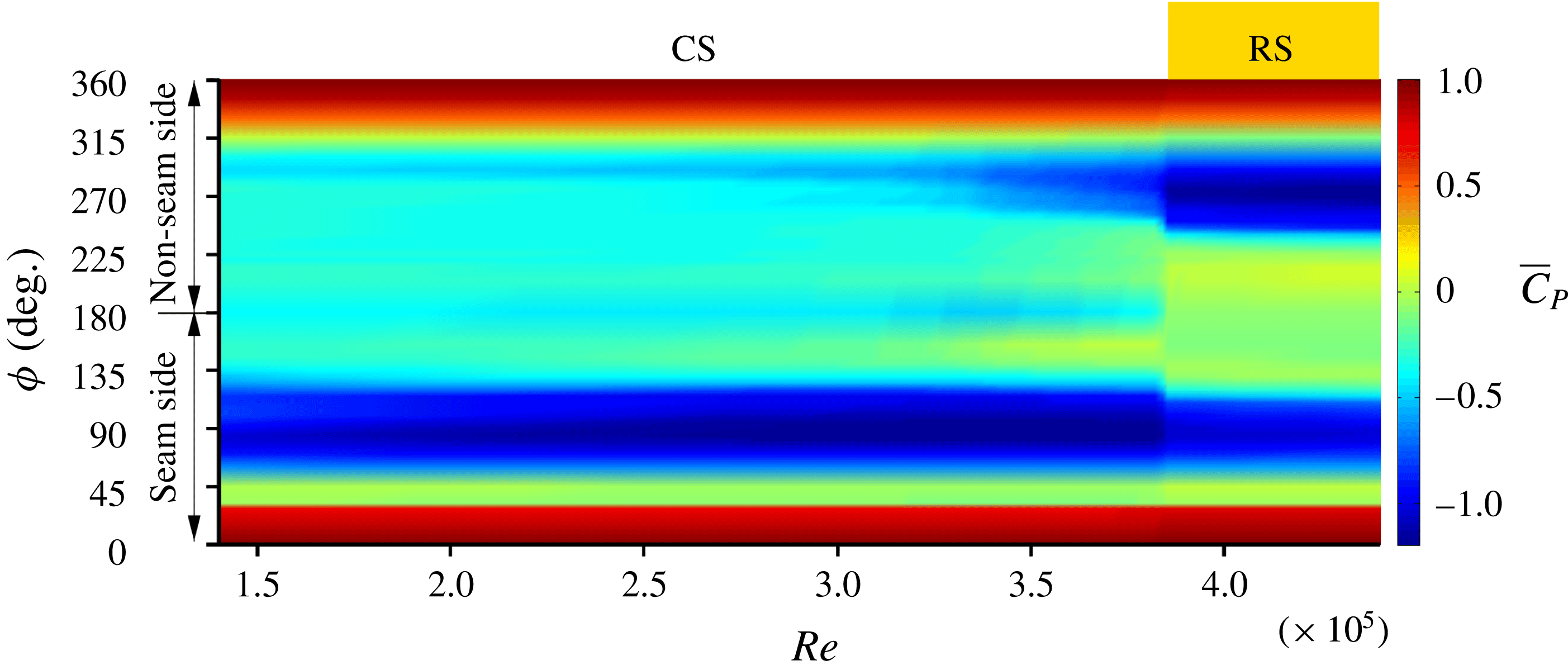
Figure 11. Flow past a sphere with one trip at $\unicode[STIX]{x1D719}_{T}=30^{\circ }$ : variation of mean coefficient of pressure on the $\unicode[STIX]{x1D719}$ – $Re$ plane. The data presented here have been acquired from the pressure ports lying on the circumferential line C (shown in figure 4).

3.6 Surface-pressure measurements

Figure 11 shows the angular distribution of time-averaged pressure coefficient ( $\overline{C}_{P}$ ) with $Re$ for the sphere with one trip, along the circumferential line C (figure 4). The asymmetry in the surface-pressure distribution between the seam and non-seam sides, in the CS and RS flow regimes, is clearly visible. The changes in $\overline{C}_{P}$ from the CS to RS regime occur over a relatively narrow range of $Re$ . This is consistent with the variation of coefficient of forces acting on the ball with $Re$ (figure 7). To highlight some of the salient features of the flow, the line plots of $\overline{C}_{P}$ with $\unicode[STIX]{x1D719}$ are shown in figure 12(a) at certain $Re$ . An interesting observation from figure 12(a) is the resemblance in the pressure distribution on the non-seam side with that on the smooth sphere (from Deshpande et al. Reference Deshpande, Kanti, Desai and Mittal2017), for a comparable  $Re$ .

Figure 12. Angular distribution of time-averaged pressure coefficient ( $\overline{C}_{P}$ ) on a sphere with one trip at $\unicode[STIX]{x1D719}_{T}=30^{\circ }$ (lines) and a smooth sphere (○) at various $Re$ : (1)  $1.64\times 10^{5}$ , (2)  $1.91\times 10^{5}$ , (3)  $2.18\times 10^{5}$ , (4)  $2.45\times 10^{5}$ , (5)  $2.86\times 10^{5}$ , (6)  $3.26\times 10^{5}$ , (7)  $3.52\times 10^{5}$ , (8)  $3.83\times 10^{5}$ , (9)  $4.23\times 10^{5}$ and (10)  $4.43\times 10^{5}$ . The data for a sphere with one trip in (a) have been acquired from the pressure ports lying on the circumferential line C, while data in (b) have been acquired from the ports lying on the lines A–E (dashed) and B–D (solid), respectively. The shaded region indicates the approximate angular location where an LSB is observed. Triangles joined by broken lines indicate $\overline{C}_{P}$ values measured at the pressure ports just upstream and downstream of the trip.

The $\overline{C}_{P}$ distribution for $Re=1.64\times 10^{5}$ , in figure 12(a), shows a plateau on the seam side for $100^{\circ }\leqslant \unicode[STIX]{x1D719}\leqslant 115^{\circ }$ . This signifies the presence of an LSB in this region (Deshpande et al. Reference Deshpande, Kanti, Desai and Mittal2017). To understand the structure of the LSB at other non-zero polar locations on the surface of the model, the $\overline{C}_{P}$ distribution at ports located along circumferential lines A, B, D and E (figure 4 and table 2) is shown in figure 12(b).

The symmetry of the model about line C is utilized to plot data for ports on lines A ( $\unicode[STIX]{x1D703}=60^{\circ }$ ) and E ( $\unicode[STIX]{x1D703}=-60^{\circ }$ ) together and referred to as data along line A–E. The case with line B–D is similar. The size of the LSB decreases in both polar and azimuthal directions with increase in $Re$ , which is consistent with the observations from the oil-flow study. The decrease in the azimuthal direction is mostly due to the downstream shift of the location of laminar boundary layer separation, while the turbulent reattachment remains fixed at $\unicode[STIX]{x1D719}\approx 115^{\circ }$ . In terms of the variation in the polar direction, the LSB disappears from the seam side along line B–D at $Re\approx 3.26\times 10^{5}$ and then along C at a slightly higher $Re\approx 3.83\times 10^{5}$ .

For all $Re$ corresponding to the CS regime, the turbulent boundary layer separates at $\unicode[STIX]{x1D719}\approx 135^{\circ }$ on the seam side. This is inferred from the constant pressure distribution on the leeward side of the sphere. The onset of the transition of the boundary layer on the non-seam side of the model marks the beginning of the RS regime. Figure 12(a) shows the presence of an LSB on the non-seam side for $Re=4.23\times 10^{5}$ and $4.43\times 10^{5}$ . The reattached boundary layer eventually separates at $\unicode[STIX]{x1D719}\approx 225^{\circ }$ , leading to a significant increase in suction over the non-seam side. The azimuthal location of the separation point on the seam side changes, from $\unicode[STIX]{x1D719}\approx 135^{\circ }$ (CS) to $\unicode[STIX]{x1D719}\approx 125^{\circ }$ (RS) (figures 11 and 12), during the switch from CS to RS. It leads to loss in peak suction on the seam side of the model and further adds to the magnitude of the swing force towards the non-seam side.

The variation of the relative suction, between the seam and non-seam sides, with $Re$ is particularly interesting (figures 11 and 12 a). It undergoes a sharp change during the CS–RS transition. We define the difference between the $\overline{C}_{P}$ distribution on the two sides as: $\unicode[STIX]{x0394}\overline{C}_{P}(\unicode[STIX]{x1D719})=[(\overline{C}_{P})_{s}(\unicode[STIX]{x1D719})-(\overline{C}_{P})_{ns}(\unicode[STIX]{x1D719})]$ . Its variation along line C, for various $Re$ , is shown in figure 13 and is useful in understanding the lateral force experienced by the model. We note that a negative value of $\unicode[STIX]{x0394}\overline{C}_{P}(\unicode[STIX]{x1D719})$ implies a higher suction on the seam side (i.e. a positive $C_{Z}$ ). Similarly, a positive value corresponds to a larger relative suction on the non-seam side (i.e. a negative  $C_{Z}$ ).

Figure 13. (a) A schematic for defining $\unicode[STIX]{x0394}\overline{C}_{P}$ . (b) Angular distribution of $\unicode[STIX]{x0394}\overline{C}_{P}$ along the circumferential line C of the sphere with one trip at various $Re$ : (1)  $1.64\times 10^{5}$ , (4)  $2.45\times 10^{5}$ , (6)  $3.26\times 10^{5}$ , (8)  $3.83\times 10^{5}$ , (9)  $4.23\times 10^{5}$ and (10)  $4.43\times 10^{5}$ . The plots follow the same legend as used in figure 12. Symbols joined by broken lines indicate $\overline{C}_{P}$ values measured at the pressure ports just upstream and downstream of the trip.

The $\unicode[STIX]{x0394}\overline{C}_{P}$ – $\unicode[STIX]{x1D719}$ distribution is virtually identical for all the $Re$ in the regime of RS. In the regime of CS, it is again insensitive to $Re$ , except in the region downstream of the shoulder, where the change is associated with the activity related to the LSB (figure 12). As the $Re$ increases in the CS regime, the decrease in $\unicode[STIX]{x0394}\overline{C}_{P}$ in the range $90^{\circ }<\unicode[STIX]{x1D719}<120^{\circ }$ is accompanied by its increase in $135^{\circ }<\unicode[STIX]{x1D719}<155^{\circ }$ . Therefore, in both the CS and RS regimes the lateral force coefficient is largely constant with $Re$ (figure 7). It is also observed that the net differential suction is larger in the CS regime as compared to that in the RS regime. This is consistent with the force experienced by the model in the CS ( $\overline{C}_{Z}\sim 0.35$ ) and RS ( $\overline{C}_{Z}\sim -0.15$ ) regimes. An interesting observation from figure 13(b) is that the peak of the relative suction in the CS regime is just upstream of the shoulder while it is at $\unicode[STIX]{x1D719}\approx 120^{\circ }$ in the RS regime (figure 13 a). In the CS regime, the primary contribution to $\unicode[STIX]{x0394}\overline{C}_{P}$ is from the high relative suction in the shoulder region on the seam side. On the other hand, in the RS regime, the main difference is the presence of a prominent LSB on the non-seam side as opposed to its absence/reduced size on the seam side.

3.7 Switch between the flow regimes: intermittency of the LSB

The switch between the flow regimes, for example CS to RS, is explored. Figures 6, 7 and 11 suggest that the transition from CS to RS is caused by the formation of an LSB on the non-seam side. This observation raises a question: Does the LSB, on the model sphere with a trip, involve intermittency (Deshpande et al. Reference Deshpande, Kanti, Desai and Mittal2017) during the early stages of transition? The middle row of figure 14 shows the time variation of $C_{D}$ and $C_{Z}$ for the model with one trip at $Re=3.83\times 10^{5}$ . This $Re$ lies in the very narrow band of $Re$ where the flow transitions from the CS to RS regime (figures 7 and 12). The time histories of both $C_{D}$ and $C_{Z}$ show an intermittent transition between bistable states: a positive $C_{Z}$ (CS) and negative $C_{Z}$ (RS). Also shown for reference are the time histories of $C_{D}$ and $C_{Z}$ for $Re=3.68\times 10^{5}$ and $3.92\times 10^{5}$ corresponding to CS and RS states, respectively.

Figure 14. Time histories of $C_{D}$ (a,c,e) and $C_{Z}$ (b,d,f) for flow past a sphere with one trip at $\unicode[STIX]{x1D719}_{T}=30^{\circ }$ at $Re=3.68\times 10^{5}$ (a,b), $3.83\times 10^{5}$ (c,d) and $3.92\times 10^{5}$ (e,f). The CS and RS flow regimes are indicated by white and off-white background colours, respectively.

Figure 15. Distribution of the coefficient of pressure ( $C_{P}$ ) on the surface of the sphere with one trip at $Re=3.83\times 10^{5}$ and $\unicode[STIX]{x1D719}_{T}=30^{\circ }$ for the pressure ports lying on the circumferential line C. (a) Space–time diagram of $C_{P}$ . Also marked are the regimes corresponding to CS and RS. (b) Angular distribution of the conditional time-averaged pressure coefficient for states CS ( $\langle C_{P}\rangle _{CS}$ , triangles) and RS ( $\langle C_{P}\rangle _{RS}$ , squares). Also shown is the time-averaged $C_{P}$ ( $\overline{C}_{P}$ , circles). The approximate angular location where an LSB is observed in the flow state corresponding to RS is indicated via shading.

Figure 15(a) shows the space–time diagram of the $C_{P}$ distribution on the circumferential line C for $Re=3.83\times 10^{5}$ . The $C_{P}$ distribution also exhibits a switch between bistable states. The CS and RS states are identified in figure 15(a) via the relative strength of the suction on two points on the shoulder corresponding to $\unicode[STIX]{x1D719}=90^{\circ }$ (seam side) and $270^{\circ }$ (non-seam side). Conditional averaging of the $C_{P}$ distribution is carried out for the CS and RS states. These values are referred to as $\langle C_{P}\rangle _{CS}$ and $\langle C_{P}\rangle _{RS}$ , respectively. Figure 15(b) shows these conditionally averaged distributions as well as the time-averaged distribution for the entire duration of measurement ( $\overline{C}_{P}$ ). A plateau is observed in the $\langle C_{P}\rangle _{RS}$ distribution for approximately $240^{\circ }\leqslant \unicode[STIX]{x1D719}\leqslant 255^{\circ }$ . This suggests the presence of an LSB on the non-seam side for the time duration when the flow is in the state of RS. Such a plateau is not observed in the distribution for $\langle C_{P}\rangle _{CS}$ or that for $\overline{C}_{P}$ , reaffirming that the CS–RS transition is a consequence of the formation of an LSB on the non-seam side. We also note that none of the three distributions suggest an LSB on the seam side, which is consistent with figures 9 and 12. Figure 15 brings out the difference in the azimuthal location of the final separation point between the CS and RS states. It shows that the turbulent flow separation point on the seam side moves upstream as the flow switches from CS to RS.

Intermittency of the LSB is also observed at the onset of transition of the CS regime. A detailed analysis was carried out for the instantaneous force coefficients recorded for the model sphere with five trips at $Re=0.6\times 10^{5}$ (not shown here). The analysis confirmed the intermittent nature of the LSB on the seam side. In this case, $C_{Z}$ exhibits alternate switching between two mean states: (i) a state devoid of an LSB and with zero lateral force ( $\langle C_{Z}\rangle _{NS}=0$ ), and (ii) a state with an LSB on the seam side and positive lateral force ( $\langle C_{Z}\rangle _{CS}\approx 0.24$ ).

3.8 Flow past a rough cricket ball

Figure 16. Variation of (a) $\overline{C}_{D}$ and (b) $\overline{C}_{Z}$ with $Re$ for a new and a roughened cricket ball. In all cases the trip/seam angle with the free stream is $\unicode[STIX]{x1D719}_{T}=30^{\circ }$ . Positive values of $\overline{C}_{Z}$ correspond to CS, while negative values lead to RS. (c) Schematic of the various states of the cricket ball: (i) new ball, (ii) roughened seam side (case S–R), (iii) roughened non-seam side (case NS–R) and (iv) completely roughened cricket ball (case C–R). The seam is also roughened in cases S–R and NS–R.

The effect of roughness on the force on a cricket ball is studied for $\unicode[STIX]{x1D719}_{T}=30^{\circ }$ . Figure 16 shows the variation of $\overline{C}_{D}$ and $\overline{C}_{Z}$ with $Re$ for a new ball, a ball with seam side rough (S–R), a ball with non-seam side rough (NS–R) and a completely rough ball (C–R). Figure 16 also shows the schematic of the various cases. Although a different specimen of the SG Test cricket ball was used for this set of experiments, the variation of the force coefficients for the new ball (figure 16) is in reasonable agreement with those shown in figure 6. Compared to a new ball, the model S–R begins to swing (CS) at a lower $Re$ . The peak $\overline{C}_{Z}$ for CS is approximately $0.25$ and is lower than that for a new ball ( ${\sim}0.35$ ). As suggested by Achenbach (Reference Achenbach1974) for a rough sphere, perhaps an LSB does not form on the roughened seam side, leading to an upstream location of the transition of the boundary layer compared to that on the new ball. This leads to reduced asymmetry in the pressure distribution on the two halves and, therefore, a lower peak force coefficient for CS. The switch from CS to RS is abrupt and occurs at an $Re$ similar to that for a new ball. The peak magnitude for RS, however, is significantly larger ( ${\sim}0.22$ ) as compared to the new ball ( ${\sim}0.15$ ). This is because the turbulent boundary layer on the roughened seam side separates at a relatively upstream location compared to that for a new ball. This creates larger asymmetry in the pressure for the S–R model in the RS regime. It also leads to a wider wake and, therefore, a larger $\overline{C}_{D}$ .

The flow past model NS–R is very interesting; the roughness on the non-seam side appears to be more effective than the seam (on the seam side) in causing the transition of the boundary layer. Therefore, unlike a new ball, the transition of the boundary layer occurs first on the non-seam side. As a result, the NS–R model undergoes a switch from NS to RS directly, and at a fairly low $Re$ (figure 16). The transition on the seam side is similar to that for a new ball. The $\overline{C}_{D}$ value decreases with increase in $Re$ up to $Re\sim 1.0\times 10^{5}$ . This marks the completion of transition of the boundary layer on both halves of the ball. As suggested by Achenbach (Reference Achenbach1974) for a rough sphere, further increase in $Re$ causes gradual upstream movement of the transition and separation points on the roughened non-seam side of the ball. This results in a very gradual increase in $\overline{C}_{D}$ as well as $\overline{C}_{Z}$ with increase in  $Re$ .

The sequence of onset of CS and RS for the completely roughened (C–R) model is the same as that for a new ball, but each event occurs at a significantly lower $Re$ . This is consistent with our earlier observation related to figure 7 wherein the CS–RS transition for a new ball, owing to its inherent surface roughness, occurs at a relatively lower $Re$ compared to a sphere with trip(s). The value of $\overline{C}_{D}$ decreases and $\overline{C}_{Z}$ increases with increasing $Re$ for $Re<0.7\times 10^{5}$ (figure 16), suggesting that the transition on the seam side of the ball leads to CS. As expected, the peak $\overline{C}_{Z}$ is the same as that for model S–R; it is lower than that for a new ball. The change from CS to RS is due to the transition of the boundary layer on the non-seam side. It is abrupt (at $Re\sim 1.0\times 10^{5}$ ) and is accompanied by a significant fall in $\overline{C}_{D}$ . Both $\overline{C}_{D}$ and $\overline{C}_{Z}$ are close to their minimum values at this $Re$ , signifying a complete transition of the boundary layer on the non-seam side. The peak magnitude of $\overline{C}_{Z}$ for RS for this case is smaller than that for the model NS–R. This is due to laminar separation, at the corresponding $Re$ , for model NS–R, and a turbulent separation for the model C–R, on the seam side of the respective models. Further increase in $Re$ leads to upstream movement of the transition and separation points on the non-seam side of the model C–R leading to increase in $\overline{C}_{D}$ and $\overline{C}_{Z}$ . The azimuthal location of the separation point of the flow on the seam and non-seam sides is nearly the same at $Re\sim 2.0\times 10^{5}$ , leading to $\overline{C}_{Z}\sim 0$ . The model undergoes CS, albeit of low magnitude, with further increase in  $Re$ .

3.9 Trajectory of a cricket ball

We estimate the trajectory of a new as well as rough balls, delivered at a certain initial speed and seam orientation, by integrating the following equation in time: $m(\text{d}\boldsymbol{V}/\text{d}t)=\boldsymbol{F}$ . Here, $m$ is the mass of the cricket ball, $\boldsymbol{V}$ its velocity and $\boldsymbol{F}$ the force acting on it. We restrict our attention to the motion of the ball in a horizontal plane and assume that the ball maintains its initial seam position throughout its trajectory and is devoid of any spin. We note that $\overline{C}_{Y}\approx 0$ for a non-spinning ball. In reality, a swing bowler would typically impart back-spin on the ball, leading to non-zero $\overline{C}_{Y}$ . In this work, we do not consider the motion of the ball in the vertical plane. The interested reader may refer to the work by Baker (Reference Baker2010), which presents the vertical trajectory of the ball solely due to the action of gravity. The lateral component of velocity of the ball at the time of delivery is assumed to be zero. It is further assumed that the aerodynamic force acting on the ball at each time instant is the time-averaged force on the ball for the fully developed flow at the corresponding value of instantaneous $Re$ . The force measurements from the wind-tunnel testing of the SG Test cricket ball are utilized to estimate $\boldsymbol{F}$ . Assuming that the ambient conditions correspond to normal temperature and pressure ( $20\,^{\circ }$ C, 1 atm), the variation of lateral force and drag with speed, for a new and roughened SG Test cricket ball of diameter 71 mm, are shown in figures 17 and 18. Force $\boldsymbol{F}$ at each time instant is estimated by interpolating the data for the corresponding $Re$ from these figures. The mass of the ball is assumed to be the same as that of the standard SG Test cricket ball ( $=0.156~\text{kg}$ ). A time step of 0.001 s is utilized to integrate the equation of motion.

Figure 17. Variation of time-averaged (a) swing force ( $\overline{F}_{Z}$ ) and (b) drag force ( $\overline{F}_{D}$ ) with speed (km h $^{-1}$ ) measured for a new cricket ball oriented at various seam angles  $\unicode[STIX]{x1D719}_{T}$ .

Figure 18. Variation of time-averaged (a) swing force ( $\overline{F}_{Z}$ ) and (b) drag force ( $\overline{F}_{D}$ ) with speed (km h $^{-1}$ ) measured for a new as well as roughened cricket balls oriented at a seam angle $\unicode[STIX]{x1D719}_{T}=20^{\circ }$ .

3.9.1 New cricket ball

We observe from figure 17 that the variation of the drag and lateral force with speed is qualitatively similar for all $\unicode[STIX]{x1D719}_{T}$ . Its main effect is the speed at which NS switches to CS, and CS to RS. Of the three seam orientations considered, the CS–RS change-over occurs at the lowest speed for $\unicode[STIX]{x1D719}_{T}=20^{\circ }$ . It has been shown by Mehta (Reference Mehta1985) that $\unicode[STIX]{x1D719}_{T}=20^{\circ }$ is the optimum angle for swing bowling. Figure 19 shows the streamwise speed of the ball and its lateral movement as it travels down the pitch of length 22 yards ( ${\approx}20.12~\text{m}$ ), for $\unicode[STIX]{x1D719}_{T}=20^{\circ }$ and various initial speeds. The streamwise speed of the ball, during its travel to the end of the pitch, decreases by 11.9 % when its initial speed is 90 km h $^{-1}$ and by 9.2 % when the initial speed is 165 km h $^{-1}$ . This is consistent with the results of Baker (Reference Baker2010), who reported a decrease of 8–13 % for initial speeds lying between 90 and 153 km h $^{-1}$ . The initial speed of the ball has a very significant effect on its trajectory. The ball experiences CS at relatively low initial speeds and RS at higher speeds. The trajectories of the balls delivered at speeds corresponding to the CS regime are similar to those reported by Mehta (Reference Mehta2005). Also shown are the measurements by Imbrosciano (Reference Imbrosciano1981) for a cricket ball delivered at an approximate initial speed of 108 km h $^{-1}$ . The streamwise variation of the lateral movement of the ball is in reasonable agreement with the present estimates.

Figure 19. Variation of the (a) streamwise speed and (b) lateral deviation of the ball as it moves along the pitch length. The estimates are for a ball delivered at different initial speeds. In all cases it is assumed that the ball maintains a seam angle of $\unicode[STIX]{x1D719}_{T}=20^{\circ }$ . Also shown in (b) is the lateral deviation measured by Imbrosciano (Reference Imbrosciano1981) for a ball delivered at 108 km h $^{-1}$ .

Figure 20. Variation of the (a) streamwise speed and (b) lateral deviation of the ball as it moves along the pitch length for various seam angles ( $\unicode[STIX]{x1D719}_{T}$ ). The initial speed of the ball is 146 km h $^{-1}$ .

To bring out the very significant role of the orientation of the seam, and the various types of possible trajectories, figure 20 shows the lateral deflection of the ball delivered at 146 km h $^{-1}$ , for three values of $\unicode[STIX]{x1D719}_{T}$ . The ball with $\unicode[STIX]{x1D719}_{T}=10^{\circ }$ undergoes CS while the one with $\unicode[STIX]{x1D719}_{T}=20^{\circ }$ exhibits RS. The case of $\unicode[STIX]{x1D719}_{T}=30^{\circ }$ is very interesting. At this speed, on its release, the ball experiences a lateral force towards the non-seam side and undergoes RS. After travelling approximately 13 m down the pitch, it slows down enough to get into the regime of CS and encounters a change in the direction of lateral aerodynamic force; it now acts in the direction of seam. This causes it to undergo CS for the remaining duration of its flight. A near 10 % decrease in the streamwise speed of the ball enables the switch from the RS to CS regime, leading to such a trajectory. A similar trajectory may be observed for all seam orientations, albeit at different speeds of the delivery of the ball. Such trajectories have also been reported by Baker (Reference Baker2010) for an old/rough cricket ball.

Figure 21. The lateral deviation of the ball when it reaches the end of the pitch for various speeds at the time of its delivery. In all cases it is assumed that the ball maintains a seam angle of $\unicode[STIX]{x1D719}_{T}=20^{\circ }$ .

An important parameter is the effective lateral movement of the ball between the time it is released from one end of the pitch to that when it reaches the other end. Figure 21 shows the variation of the lateral deflection of the ball with its initial speed for $\unicode[STIX]{x1D719}_{T}=20^{\circ }$ . The ball does not undergo any lateral movement when it is delivered at speeds lower than approximately 30 km  $\text{h}^{-1}$ . It exhibits CS for 30–119 km  $\text{h}^{-1}$ and RS for ${>}125~\text{km}~\text{h}^{-1}$ . The ball exhibits both RS and CS when delivered in the speed range 119–125 km  $\text{h}^{-1}$ . This speed range has also been marked in figure 21. The speeds for the onset of CS and RS for a new cricket ball, in the present study, are slightly lower than those observed by Mehta (Reference Mehta2005). This is possibly due to the different brand of cricket balls used in the two studies. The deliveries which undergo both RS and CS correspond to the velocity range where the lateral force $C_{Z}$ reverses direction (figure 17) with decrease in speed. The trajectory of the ball for two such speeds (120 and 125 km h $^{-1}$ ) lying within this narrow band are shown in figure 19(b). The delivery bowled at 120 km h $^{-1}$ undergoes a ‘late’ swing. The lateral force on the ball, in the initial stage of its trajectory, is very low (figure 17). With decrease in its speed of the order of 10 % (figure 19 a), the flow switches from RS to CS, resulting in a significantly larger swing force during the later part of its trajectory. Although, the net lateral displacement of the ball is relatively low in this regime, it is particularly difficult for the batsman to anticipate such a trajectory of the ball.

3.9.2 Rough cricket ball

Figure 22. The lateral deviation of the ball when it reaches the end of the pitch for various initial speeds. The thick dashed lines represent CS while the thin dashed lines show the speed range where the ball experiences RS. The speed range corresponding to the deliveries that exhibit both RS and CS during their flight is highlighted by a thicker shaded line for each configuration. The speed range for the NS regime is shown as a dotted line.

Trajectory analysis is carried out for the models S–R, NS–R and C–R for $\unicode[STIX]{x1D719}_{T}=20^{\circ }$ using the data for aerodynamic forces acting on the ball presented in figure 18. Figure 22 shows the variation, with its initial speed, of the lateral deflection of the ball, at the far end of the pitch. Also shown is the deflection for a new ball. The speed for the onset of CS is lowest for S–R and C–R models and largest for the NS–R model. The peak lateral deflection during CS is largest for the new ball and lowest for the completely rough (C–R) ball. Interestingly, the initial speed of the ball that leads to peak deflection during CS is lowest for C–R, followed by NS–R, S–R and new ball. An interesting point brought out by figure 22 is that the speed of delivery of the ball that achieves maximum lateral movement, during CS, depends on the condition of the ball. A fast bowler would be an ideal choice with a new ball; a relatively slower bowler would achieve CS more effectively with a completely roughened ball (C–R). It is noted that the NS–R and C–R models exhibit CS for two ranges of speeds. The deflection in the higher range of speeds is significantly smaller than in the lower range.

Both new and C–R balls lead to comparable peak lateral movement during RS, although at different speeds. The new ball reverses at very high speed while the C–R model exhibits similar RS at relatively low speed. The range of initial speed that leads to RS for various models at $\unicode[STIX]{x1D719}_{T}=20^{\circ }$ is 59–141 km h $^{-1}$ for C–R, 98–133 km h $^{-1}$ for NS–R, ${>}117~\text{km}~\text{h}^{-1}$ for S–R and ${>}125~\text{km}~\text{h}^{-1}$ for the new ball. The lowest speed for the ball to undergo RS is smallest for C–R, followed by NS–R, S–R and a new ball.

The deliveries that exhibit both RS and CS, for a new ball (119–125 km h $^{-1}$ ) as well as S–R model (111–117 km h $^{-1}$ ), occur in a very narrow and comparable range of initial speed. Interestingly, for the NS–R and C–R models (at $\unicode[STIX]{x1D719}_{T}=20^{\circ }$ ), similar trajectories can occur in two ranges of speed. For example, for the NS–R model, the ball first moves away from the seam and then towards the seam when delivered in the speed range 94–98 km h $^{-1}$ . It will exhibit both CS and RS again when delivered in the speed range 133–138 km h $^{-1}$ . However, this time the nature of deflection is the reverse of the former; the ball initially moves towards the seam and after it has slowed down it moves away from the seam. The range of speeds for similar trajectories of the C–R ball is 56–59 km h $^{-1}$ and 141–146 km h $^{-1}$ , respectively. An interesting observation from figure 22 is that the lateral movement for the C–R ball is relatively small when delivered at a speed in excess of 120 km h $^{-1}$ . Figure 22 also shows the variation, with speed, of the lateral deflection of the NS–R ball at $\unicode[STIX]{x1D719}_{T}=30^{\circ }$ . This variation is starkly different compared to that at $\unicode[STIX]{x1D719}_{T}=20^{\circ }$ . For $\unicode[STIX]{x1D719}_{T}=30^{\circ }$ , the roughness of the non-seam side leads to a direct transition from NS to RS at fairly low $Re$ . The transition to CS occurs on further increasing the speed.